the Creative Commons Attribution 4.0 License.
the Creative Commons Attribution 4.0 License.
 | 15 Jan 2024
Assessing sampling and retrieval errors of GPROF precipitation estimates over the Netherlands
Hidde Leijnse
Aart Overeem
Remko Uijlenhoet
The Goddard Profiling algorithm (GPROF) converts radiometer observations from Global Precipitation Measurement (GPM) constellation satellites into precipitation estimates. Typically, high-quality ground-based estimates serve as reference to evaluate GPROF's performance. To provide a fair comparison, the ground-based estimates are often spatially aligned to GPROF. However, GPROF combines observations from various sensors and channels, each associated with a distinct footprint. Consequently, uncertainties related to the representativeness of the sampled areas are introduced in addition to the uncertainty when converting brightness temperatures into precipitation intensities. The exact contribution of resampling precipitation estimates, required to spatially and temporally align different resolutions when combining or comparing precipitation observations, to the overall uncertainty remains unknown. Here, we analyze the current performance of GPROF over the Netherlands during a 4-year period (2017–2020) while investigating the uncertainty related to sampling. The latter is done by simulating the reference precipitation as satellite footprints that vary in size, geometry, and applied weighting technique. Only GPROF estimates based on observations from the conical-scanning radiometers of the GPM constellation are used. The reference estimates are gauge-adjusted radar precipitation estimates from two ground-based weather radars from the Royal Netherlands Meteorological Institute (KNMI). Echo top heights (ETHs) retrieved from the same radars are used to classify the precipitation as shallow, medium, or deep. Spatial averaging methods (Gaussian weighting vs. arithmetic mean) minimally affect the magnitude of the precipitation estimates. Footprint size has a higher impact but cannot explain all discrepancies between the ground- and satellite-based estimates. Additionally, the discrepancies between GPROF and the reference are largest for low ETHs, while the relative bias between the different footprint sizes and implemented weighting methods increase with increasing ETHs. Lastly, our results do not show a clear difference between coastal and land simulations. We conclude that the uncertainty introduced by merging different channels and sensors cannot fully explain the discrepancies between satellite- and ground-based precipitation estimates. Hence, uncertainties related to the retrieval algorithm and environmental conditions are found to be more prominent than resampling uncertainties, in particular for shallow and light precipitation.
- Article
(3878 KB) - Full-text XML
- BibTeX
- EndNote


Accurate global precipitation estimates are vital for both hydrological research and operational applications like weather forecasts and flood early warning systems. Accurate estimates can be retrieved from well-established ground-based observations, such as weather radars and rain gauges. Their spatial coverage and representation, however, are limited (Lorenz and Kunstmann, 2012; Saltikoff et al., 2019). This limitation can be overcome with the implementation of spaceborne sensors. Yet, to date, precipitation estimates retrieved from spaceborne sensors are not as accurate as those derived from ground-based sensors (Chen and Li, 2016; Tang et al., 2020; Maggioni et al., 2022).
Determining the state-of-the-art accuracy of satellite-based estimates over different surface types and in various climates is crucial to further improve the performance of spaceborne retrieval algorithms (Maggioni et al., 2016; Kim et al., 2017). Retrieval algorithms use physical and/or statistical relations to convert spaceborne observations to precipitation estimates at the Earth’s surface. Their input is either indirectly (observation of cloud properties) or more directly (observation of hydrometeor properties) related to precipitation (Prigent, 2010; Kidd and Huffman, 2011; Skofronick-Jackson et al., 2018a).
The spatiotemporal resolution of indirect observations, retrieved from sensors aboard geostationary satellites, is higher than that of more direct observations, retrieved from radiometers aboard low-orbiting (LEO) satellites (Chang and Hong, 2012; Maggioni et al., 2016; Sun et al., 2018). Still, the latter are preferred for quantitative applications in meteorology and hydrology as precipitation retrieval from visible and infrared channels is based on cloud-to-precipitation relations. These statistical relations are location and time-dependent and generate precipitation estimates with poor accuracy (Lee et al., 2015; Kidd and Levizzani, 2019). In contrast, the upwelling radiation from the Earth’s surface observed by radiometers is directly affected by precipitation (Kidd and Huffman, 2011; Maggioni et al., 2016; Kidd et al., 2021b). Precipitation increases microwave emissions measured by the lower-frequency channels and decreases microwave emissions measured by the higher-frequency channels (Kummerow, 2020).
One algorithm that converts microwave emissions, often expressed as brightness temperatures (Tb), to precipitation estimates is the Goddard Profiling precipitation retrieval algorithm (GPROF) (Kummerow et al., 2001, 2015). GPROF is a Bayesian algorithm that uses an a priori database of Tb's, hydrometeor profiles, and surface precipitation estimates. GPROF's database is built on observations from the two sensors aboard the Global Precipitation Measurement (GPM) core satellite: the GPM Microwave Imager (GMI) and the dual-precipitation radar (DPR) (Hou et al., 2014; Skofronick-Jackson et al., 2018a). GMI is a radiometer equipped with 13 frequency channels. The combination of Tb's measured by each channel is matched to simultaneous DPR hydrometeor profiles and surface precipitation estimates (Randel et al., 2020).
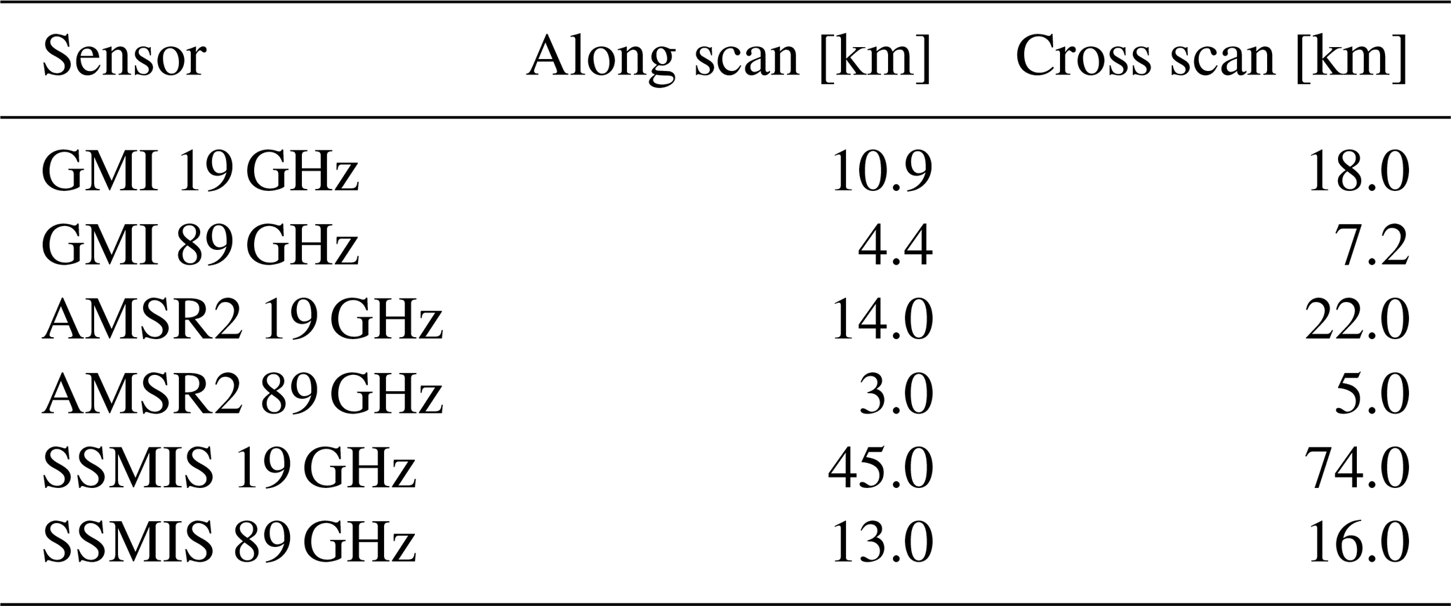
Although calibrated on GMI, GPROF is able to convert observations from all radiometers aboard GPM constellation satellites into precipitation intensities (Kummerow et al., 2015; Randel et al., 2020). However, the size of an area scanned by a radiometer, also referred to as footprint, varies with sensor and frequency channel (Guilloteau et al., 2017). For instance, the diameter of the footprint associated with the 19 GHz channel, which is often used as a “reference” resolution (You et al., 2020), is more than twice as large in both across- and along-scan directions compared to the footprint associated with the 89 GHz channel. Hence, merging various channels and sensors inevitably implies merging observations with different spatial resolutions. This difference in resolution introduces uncertainty as precipitation is highly variable in space and time (Foufoula-Georgiou et al., 2014; Cristiano et al., 2017; Leth et al., 2021). In this context, the term “uncertainty” refers to the uncertainty associated with the merged rainfall estimates due to differences in the spatial and temporal representativeness of the observations.
Up to now, research has mostly focused on the uncertainty related to assumptions in the retrieval algorithm to improve precipitation detection and accuracy of precipitation intensity. An example of a persistent challenge is the retrieval of shallow and light precipitation (Liu and Zipser, 2014; Ferraro et al., 2013; Kidd et al., 2021a; Hayden and Liu, 2021). As mentioned, large water or ice particles interact with the upwelling radiation. This interaction is weaker for shallow and light precipitation (Casella et al., 2015; Kummerow et al., 2015). Analyzing brightness temperatures of the individual frequency channels during shallow and light precipitation events reveals what radiometers do observe when those types of precipitation occur. However, as explained before, each channel is associated with a different spatial scale due to the associated footprint size. Hence, before analyzing the brightness temperatures related to each channel, the uncertainty introduced when combining or spatially aligning observations with various spatiotemporal resolutions, known as resampling, needs to be identified.
First, we briefly evaluate the most recent version of GPROF, V07, as its performance over mid-to-high latitudes has, to the best of our knowledge, not been evaluated yet. Second, we analyze to what extent the evaluation of spaceborne estimates is affected by the sampling pattern used to align the reference and spaceborne observations. Additionally, this study evaluates the uncertainty introduced when merging various footprint sizes associated with the different channels and radiometers using only reference estimates. Lastly, we determine how different characteristics, such as the vertical extent of precipitation or the proximity of the coast, affect the uncertainty related to sampling. This uncertainty is analyzed by simulating the footprints of the three conical scanners that belong to the GPM constellation. The footprints are simulated using 1 km × 1 km gauge-adjusted radar precipitation estimates provided by the Royal Netherlands Meteorological Institute (KNMI). The Netherlands, a coastal country where shallow and low-intensity precipitation frequently occurs, is used as study area from January 2017 to December 2020. Ground-based echo top heights (ETHs) are used to classify the vertical extent of precipitation within a certain footprint.
2.1 Data
The three precipitation datasets used in this study were all available over the research area, the Netherlands (50.78–53.68∘ N and 3.38–7.38∘ E; 35 000 km2), during the entire studied period, from 1 January 2017 to 31 December 2020. Each dataset is briefly described in the following subsections. An elaborate description of precipitation occurring in the research area with similar reference data partly overlapping the current research period can be found in Bogerd et al. (2021).
2.1.1 Satellite observations: GPM constellation conical scanning radiometers
The core satellite of the Global Precipitation Measurement mission (GPM) was launched in 2014. GPM aims to increase both the availability of precipitation data over ungauged areas and the understanding of precipitation processes (Hou et al., 2014; Skofronick-Jackson et al., 2017; Skofronick‐Jackson et al., 2018b). To achieve these aims, the mission consists of a constellation of satellites carrying radiometers and a “core satellite”. The core satellite carries both a radiometer with a broad spectrum of frequencies (GPM microwave imager: GMI) and a precipitation radar (DPR). This setup provides the opportunity to couple simultaneous radiometer observations and vertical precipitation structures from space. These simultaneous observations are used as input for the GPROF algorithm (Kummerow et al., 2015).
GPROF converts brightness temperatures retrieved from radiometers aboard GPM constellation satellites into precipitation estimates. GPROF is parametric: it works with all these radiometers as long as the characteristics and channel errors of each sensor are known. The algorithm is based on a Bayesian approach and uses an a priori database of observed cloud and hydrometeor profiles, based on DPR observations. These profiles are matched with simulated radiances. The radiometer observations are compared to simulated radiances to gain a weighted sum from which precipitation estimates are computed. More details about GPROF can be found in Kummerow et al. (2015), Passive Microwave Algorithm Team Facility (2022), and Randel et al. (2020). This study focused on the three conical scanning radiometers contributing to GPM: SSMIS, AMSR-2, and GMI. Their footprint sizes are shown in Table 1. The conical scanners are the most important radiometers within Integrated Multi-satellitE Retrievals for GPM (IMERG), GPM's gridded precipitation product based on GPROF estimates. IMERG selects conical scanners in case of simultaneous radiometer overpasses over a certain area.
Table 1Resolution of the three conical scanning radiometers implemented in this study.
2.1.2 Ground-based precipitation estimates: gauge-adjusted radar
The Royal Netherlands Meteorological Institute (KNMI) offers a high-quality gridded precipitation product at a spatial resolution of ∼ 1 km2 and a 5 min temporal resolution. This product is based on composites of two polarimetric C-band radars. For this product, precipitation is retrieved every 5 min by using data from scans at 3 (0.3, 1.1, and 2.0∘) out of 16 elevations from both radars. After the two radar composites are combined, the two rain gauge networks from KNMI, involving 31 automatic and 325 manual gauges, are used to adjust the radar precipitation estimates. Elaborate descriptions about this dataset can be found in Overeem et al. (2009a, b, 2011).
2.1.3 Ground-based echo top height observations: radar
Ground-based radar echo top height (ETH) data were used to classify precipitation based on its vertical extent. This classification allows us to study both to what extent the precipitation height influences the performance of GPROF and how ETH is related to precipitation variability within a certain footprint size. The ETH is defined as the maximum height at which a particular reflectivity threshold, in this case 7 dBZ, is exceeded.
The ETH observations were retrieved from the same ground-based C-band radars described in the previous subsection. However, the ETH product is based on all elevations (ranging from 0.3–12.0∘). The authors are aware of the deficiencies associated with this product. For instance, the low detection threshold of 7 dBZ combined with residual clutter and overshooting that occurs at large distances from the radar can induce unrealistically high or low ETH values. Hence, ETH observations below 1 km and above 15 km were removed before further analysis. A footprint was classified as low when 1 km ≤ ETH < 3 km, medium when 3 km≤ ETH < 6 km, and high when ETH≥6 km. The footprint is allocated to the class corresponding to the average ETH value associated with a 19 GHz footprint size. More information about the ETH product and its evaluation can be found in Beekhuis and Holleman (2008) and Aberson (2011).
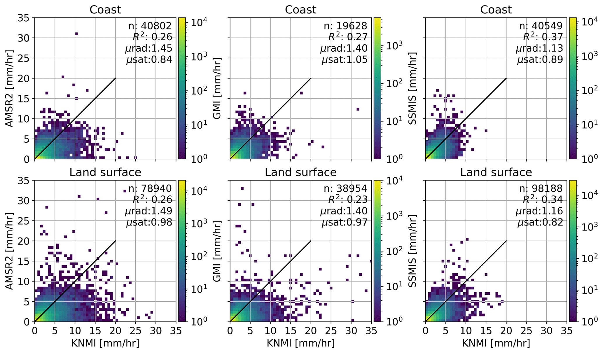
Figure 1Scatter density plots of GPROF vs. reference estimates for the entire study period (January 2017–December 2020). The first row shows observations within 20 km distance from the coast; the second row represents the remaining observations over land. The reference estimates are resampled to the footprint corresponding to the 19 GHz channel associated with the sensor (i.e., AMSR-2, GMI, SSMIS). Only paired observations where both references exceed 0.1 mm h−1 (hits) and 1 km ≤ ETH <15 km are considered.
2.2 Spatiotemporal matching
During the study period, all overpasses by the three conical scanners with more than eight pixels (i.e., individual footprints) over the land surface of the Netherlands were selected. The coordinates provided along with the satellite observations represent the center of the pixel. Subsequently, using the scan position of a particular pixel, the orientation of the elliptic-shaped footprint was determined. The scan pattern of the GMI scanner is shown in Hou et al. (2014) (Fig. 2, an example of one GMI scan is shown in light blue). The size of each footprint depends on the satellite and frequency. This study used the dimensions associated with the 19 and 89 GHz channels as these channels are considered crucial for precipitation observations as hydrometeors interact with radiation at these frequencies (Stephens and Kummerow, 2007; Kummerow, 2020). This assumption is also used within GPROF (Passive Microwave Algorithm Team Facility, 2022). Because GPROF assumes the footprint sizes of GMI, GMI's dimensions are used in this study. The high-resolution ground-based observations within each simulated footprint were averaged using either the arithmetic mean or Gaussian weighting. The uncertainty associated with the procedure to align either high-resolution reference observations with one radiometer resolution or combine various sizes of radiometer footprints to retrieve one estimate is referred to as “resampling uncertainty” in the remainder of this paper.
Additionally, footprints with center coordinates within 40 km distance of the coast were identified. The coast is highlighted because the accuracy of spaceborne precipitation retrieval over coastal areas is often reduced compared to its accuracy over land or sea/ocean (Kubota et al., 2009; Mega and Shige, 2016; Munchak and Skofronick-Jackson, 2013). This reduction is attributed to the sudden change in background radiation, which is different for land and sea/ocean. Hence, the background radiation can vary within a footprint close to the coast. However, precipitation dynamics and the difficulties to correctly capture this could also be the reason for a change in accuracy, as the temperature difference between the coast and land affects the occurrence of precipitation (and the associated precipitation types). By studying the reference estimates resampled at different scales while taking into account the proximity of the coast, we can study the sensitivity of precipitation events and their intensity as a function of coastal distance and either reject or confirm this relationship.
2.3 Validation
Established metrics were used to assess the performance of GPROF. The relative bias (RB) was calculated to determine the sign and magnitude of the bias between the evaluated product (GPROF) and the reference (ground-based precipitation estimates). A positive (negative) value indicates that the evaluated product overestimates (underestimates) the precipitation intensity compared to the reference. The normalized mean absolute error (NMAE) was calculated to demonstrate the overall error magnitude, normalized by the average of the reference values. If NMAE equals 1, GPROF values are, on average, off by the same magnitude as the reference mean. Due to its normalization, NMAE allows us to compare the performance amongst different ETH classes (higher ETH is often associated with higher precipitation intensities).
The RB and NMAE are defined as follows:
where n represents the number of pixels (in our case footprints) available, in both space and time. Additionally, the probability of detection (POD) was used to measure GPROF's ability to distinguish between wet and dry footprints using a threshold of 0.1 mm h−1. It is important to note that the probability of false alarms (POFA) could not be calculated. Only estimates corresponding with valid ETH observations were selected. A valid ETH value automatically implies that the ground-based radar measured precipitation. The POD is defined as
where “hits” means that both GPROF and the reference identify a footprint as “precipitating” (exceeding 0.1 mm h−1), and “misses” means that the reference identifies a footprint as precipitating (exceeding 0.1 mm h−1) while GPROF identifies the footprint as dry (intensity lower than 0.1 mm h−1). Lastly, the coefficient of determination (R2) was computed to indicate to which extent variations in estimates from one precipitation product (e.g. GPROF) can be explained by the variability in estimates obtained from the other precipitation product (e.g. KNMI).
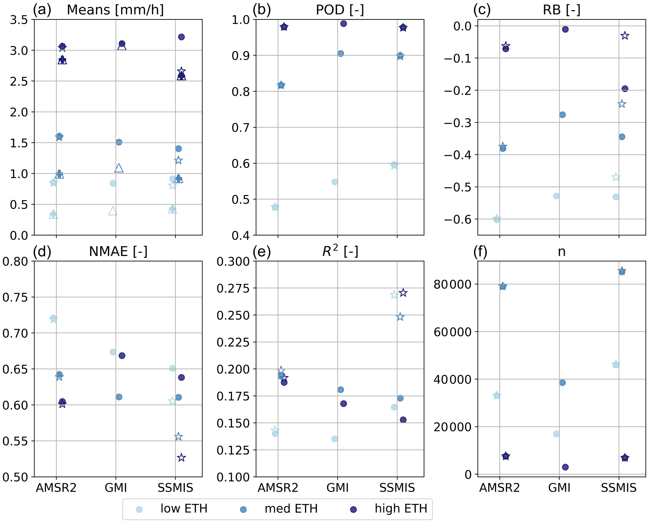
Figure 2Statistics of GPROF for the three sensors using reference estimates averaged over the footprint associated with the GMI 19 GHz channel (circles) or each sensor's own 19 GHz channel (stars). The triangles (GMI 19 GHz channel) and pluses (own sensors 19 GHz channel) in (a) represent GPROF's mean. Additionally, the vertical extent of precipitation was taken into account (different blue shades). The statistics are based on all overpasses during the study period. Except for the contingency metric (POD), paired observations where both references exceed 0.1 mm h−1 (hits) and 1 km ≤ ETH < 15 km are considered.
3.1 Evaluation of GPROF's performance
First, the performance of GPROF is determined. Coupled GPROF and reference estimates, as a function of their proximity to the coast, are shown in Fig. 1. Coupled estimates deviate from the 1:1 line in both directions, meaning GPROF both underestimates and overestimates precipitation intensity compared to the reference. In general, however, GPROF underestimates precipitation intensity as the reference mean is higher. This result is independent of the observation sensor (SSMIS, AMSR-2, or GMI) or the proximity of the coast. SSMIS-based GPROF estimates close to the coastal area have the smallest discrepancy: 0.89 vs. 1.13 mm h−1 according to the reference. GPROF can only explain 34 %–37 % of the variance observed in the reference estimates, which is even reduced to only 23 %–27 % for estimates retrieved from GMI and AMSR-2. For SSMIS and GMI, the underestimation of GPROF is worse over land, while for AMSR-2 the lowest performance is over the coastal area, especially for low-intensity events (Fig. 1, upper panel, left).
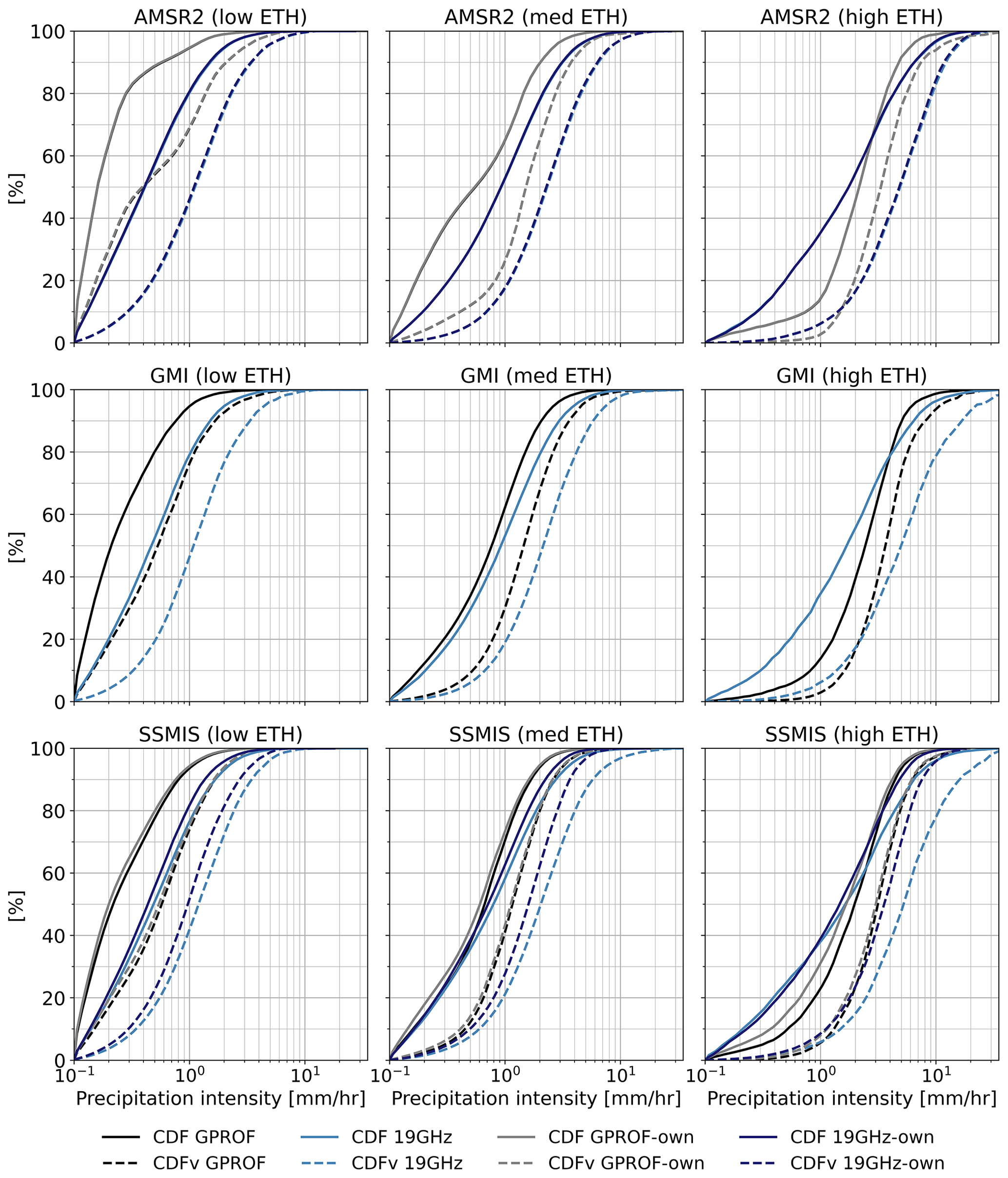
Figure 3Cumulative distribution functions of precipitation intensity occurrence (CDF: solid line) and volume (CDFv; dashed line) for GPROF (black) and the reference using the reference estimates averaged over the footprint associated with the GMI 19 GHz channel (light blue). Additionally, similar to Fig. 2, the results are also shown using the footprint associated with the 19 GHz channel of SSMIS and AMSR-2 (GPROF: grey, reference: dark blue), referred to as “own” as the native footprint size of the specific sensor was used. The sampling method and time period are the same as Fig. 2. Only paired observations where both references exceed 0.1 mm h−1 (hits) and 1 km ≤ ETH <15 km are considered. The CDFs are calculated with a logarithmic bin width. The rows represent the different sensors and the columns the different ETH classes.
Figure 2 explores the results of Fig. 1 in more detail by evaluating GPROF's performance as a function of vertical extent. The metrics are calculated with the reference resampled to the footprint size associated with the 19 GHz channel of GMI (circles) or the observing sensor (stars). Both are considered to evaluate the sensitivity of GPROF’s performance concerning the implemented method used to resample the reference. However, only observations exceeding the 0.1 mm h−1 threshold are considered. Due to different footprint dimensions, the number of observations that exceed this threshold might differ. Hence, for SSMIS and AMSR-2 two GPROF means are shown: GPROF's mean based on the observations that are coupled to reference estimates resampled to the footprint size associated with the GMI 19 GHz channel (triangles) or to the 19 GHz channel of the observing sensor (plus symbols).
Both the reference and GPROF mean increase with increasing ETH. Independent of the observation sensor (corresponding ETH) or the size of the sampled area, GPROF's mean is low compared to the reference mean, and the RB is negative. An exception is GMI observations associated with high ETH. For these observations, the reference and GPROF mean values are similar, and RB is close to zero. Additionally, GMI observations hardly ever miss precipitation associated with a high ETH, illustrated by the POD being close to 1. In contrast, the POD for shallow precipitation does not exceed 0.6 for any of the sensors, indicating that GPROF's ability to correctly detect precipitation in the case of shallow precipitation is not higher than 60 %. GPROF's enhanced performance for estimating precipitation intensity associated with high ETH compared to those associated with low ETH is less evident from the R2 and NMAE. These two statistics are less dependent on the precipitation intensity, which increases with increasing ETH. The intensity is more reflected in both RB and the mean values.
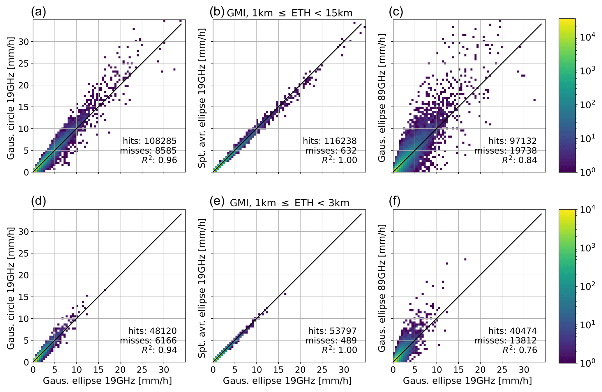
Figure 4Scatter density plots of simulated GMI observations using four sampling methods for the entire study period (January 2017–December 2020). Only paired observations where both references exceed 0.1 mm h−1 (hits) and 1 km ≤ ETH <15 km (a–c) or 1 km ≤ ETH <3 km (d–f) are considered. All scatter density plots consider the same observations. The number of hits varies due to misses by the sampling method on the y axis. The number of misses is shown in the bottom right of each panel, together with the number of hits and R2.
Figure 2 shows, as expected, that the influence of resampling is especially relevant for SSMIS observations. The SSMIS footprint is much larger, whereas AMSR-2 and GMI have similar footprint sizes (Table 1). The bias (both NMAE and RB) increases while R2 decreases when evaluating SSMIS observations against the reference resampled at GMI resolution instead of its native footprint size. This result is confirmed by Fig. 3, which shows the cumulative distribution functions (CDFs) of the occurrence of precipitation intensities (CDF, solid lines). The CDF illustrates the probability of observing values up to and including a particular precipitation intensity level. Although lower intensities occur more frequently in the Netherlands (solid lines), their contribution to the total amount of precipitation might be limited. Therefore, also the CDFv is shown, which illustrates the contribution of values up to and including a particular precipitation level to the total amount of precipitation. Figure 3 highlights the effect of using different sampling methods on the “estimated” precipitation intensity. The reference resampled to the AMSR-2 resolution (first panel, “CDF 19 GHz own”, purple) and the GMI resolution (first panel, “CDF 19 GHz”, light blue) are plotted on top of each other, implying similar results. The occurrence (solid lines) and contribution of high-intensity precipitation to the total amount of precipitation (dashed lines) are clearly reduced for reference values when resampled using the SSMIS resolution (represented by the purple color, lower panels). In general, maximum intensities increase with increasing ETH both for GPROF and the reference.
3.2 Sampling sensitivity analysis
GPROF’s performance and some first results concerning the influence of sampling on precipitation estimates are shown in Figs. 1–3. The remainder of this study concentrates on sampling only. Hence, all results are based on ground-based reference estimates averaged over various footprint sizes and geometries. Figure 4 is based on GMI coordinates and resolution and compares averaged estimates using four different sampling methods. The y axis represents, from left to right, averages of the high-resolution estimates calculated using a 19 GHz Gaussian circle, 19 GHz spatial ellipse (arithmetic average), and 89 GHz Gaussian ellipse. With “Gaus.”, we refer to Gaussian weighting.
The averaged estimates calculated using uniform weights are on the 1:1 line (middle panel), and R2 is 1 (mid panel). Although a circle results in more noise (left panel) compared to the choice of weighting, the scatter is still limited compared to the scatter observed in Fig. 1. The size of the ellipse results in the largest difference amongst the references (right panel). Estimates based on the 89 GHz channel are skewed towards higher values compared to those based on the 19 GHz channel footprints. This finding is in agreement with the results of the bottom panels of Fig. 3. The lower panel features observations associated with a shallow vertical extent. The deviations seem smaller than the deviations shown in the upper rows, likely due to the lower precipitation intensities related to shallow events. In contrast, the R2 is lower for shallow precipitation. The number of misses varies amongst the sampling methods, indicating the sampling method could (slightly) affect the POD. Again, the largest effect is the size of the sampling area, thus the channel footprint size (right panel). Still, the POD is higher than the POD of GPROF found in Fig. 2. GMI and AMSR-2 have similar footprint dimensions, resulting in similar results (not shown).
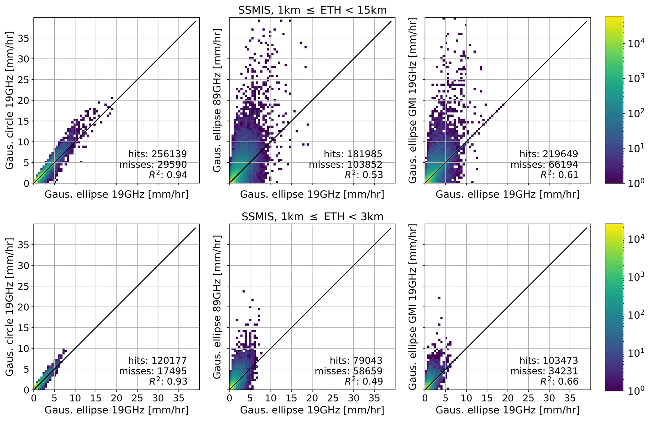
Figure 5 is similar to Fig. 4 but considers footprint dimensions based on SSMIS channels. Spatial-weighted ellipse vs. Gaussian-weighted ellipse is not shown as the results were similar to the middle panel of Fig. 4, indicating limited deviations between the two sampling methods. Hence, more emphasis has been put on the dimensions of the sampled area.
The differences between the SSMIS 19 GHz and SSMIS 89 GHz channels are larger than the differences between the SSMIS 19 GHz and GMI 19 GHz channels. Additionally, more observations are missed, and R2 is lower (R2=0.53 vs. R2=0.61). Although both footprint dimensions are smaller than the footprint dimensions associated with the SSMIS 19 GHz channel, GMI's length–width proportions are more similar to the proportions of the 19 GHz SSMIS channel. Considering only shallow observations yields similar conclusions (lower panels). The relative amount of misses is high (up to 43 %) compared to the upper row, which is comparable to GPROF's POD for shallow precipitation that was found to be independent of footprint size in Fig. 2.
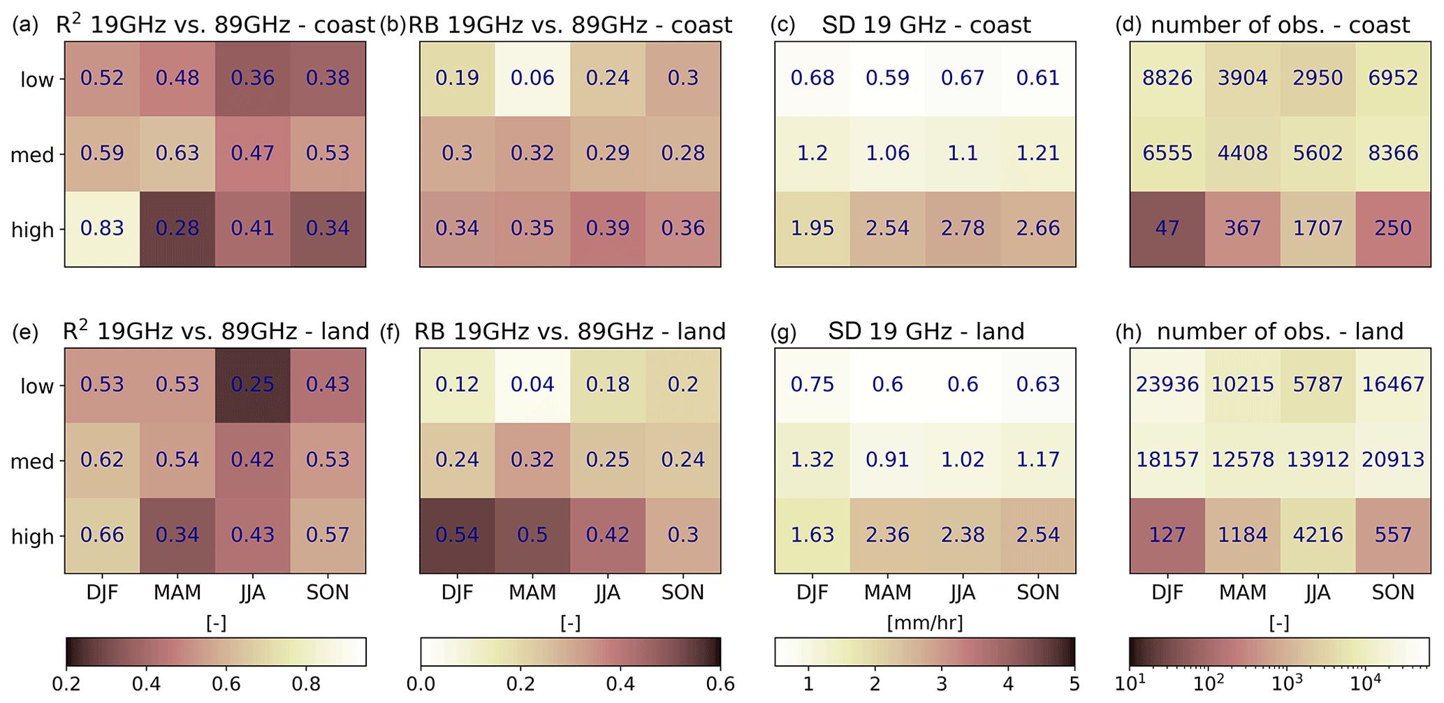
Figure 6R2, relative bias (RB), standard deviation (SD), and number of observations (n) for SSMIS observations and corresponding footprint sizes. Same observations as used in Fig. 5. Panels (a)–(d) represent the statistics of all observations within 20 km distance of the coast, and panels (e)–(h) represent those of the other observations (i.e., over land). The statistics are shown as a function of ETH and season. The background color represents the value of that particular cell. Additionally, the value itself is presented in each cell in dark blue.
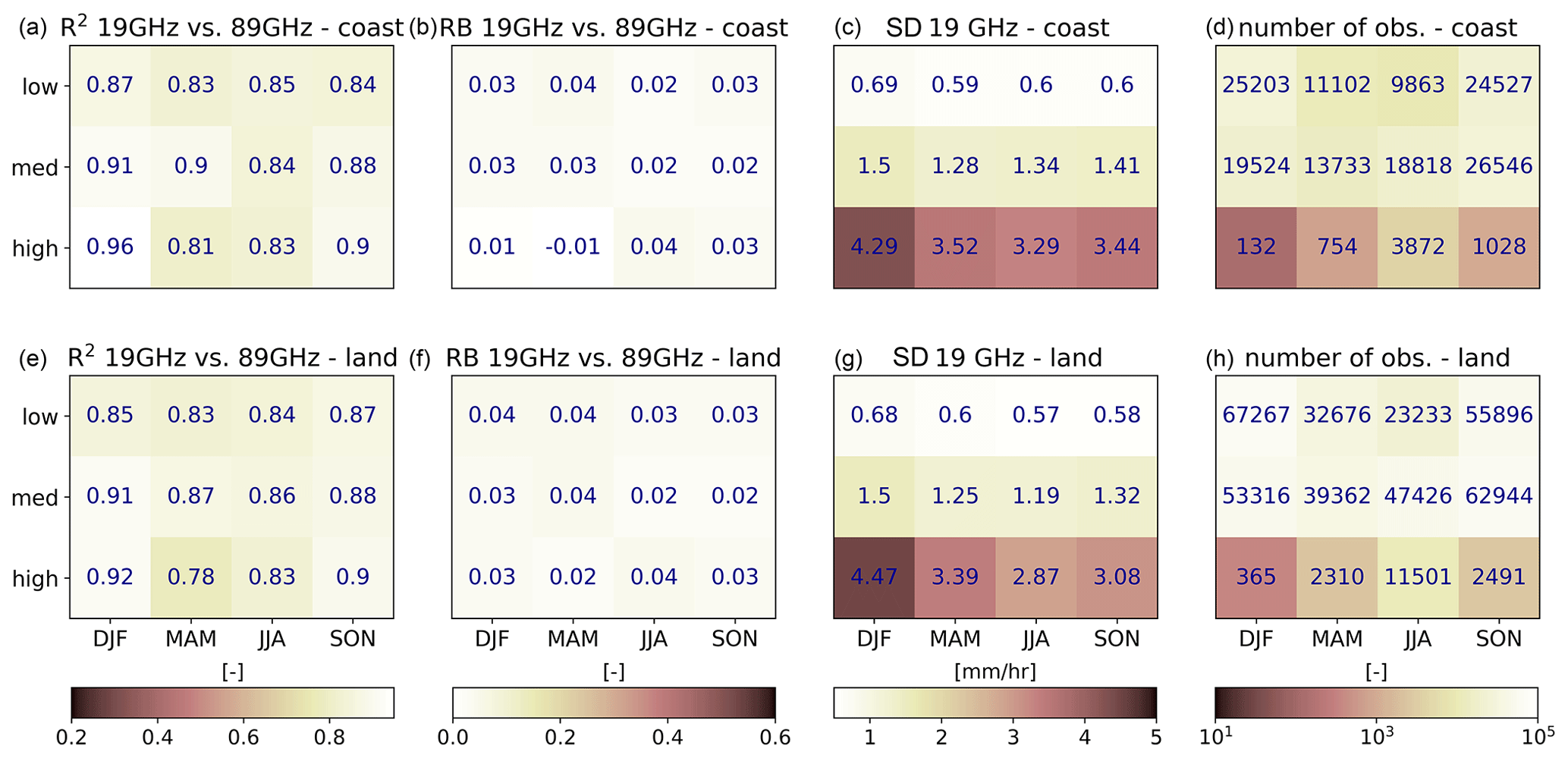
Figure 7Similar to Fig. 6 but now including all sensors and using the footprint dimensions of GMI.
Figure 5 shows large deviations in resampled reference precipitation estimates using the footprint sizes associated with the 19 and 89 GHz channels. Both channels are considered important for precipitation retrieval, especially for the GPROF algorithm. To obtain more insight into the circumstances for which the uncertainty related to merging the two channels would be largest, the observations are evaluated in more detail in Fig. 6. The observations are studied as a function of vertical extent, distance from the coast, and season. The vertical extent has a clear seasonal cycle (right panels): the occurrence of precipitation with a shallow vertical extent is highest in winter, both relative as well as in absolute numbers. High ETH frequently occurs in the summer season, while its occurrence is limited during the other seasons, especially in winter. Both the standard deviation (SD) and RB increase with increasing height, independent of season and surface type. The R2 does not exceed 0.65, except for high ETH during winter. The RB is always positive, meaning simulations with a smaller footprint result in higher precipitation estimates.
Figure 7 is similar to Fig. 6 but based on the overpasses of the three sensors. All observations are resampled to footprint sizes associated with GMI's 19 or 89 GHz channels to increase the sample size (the results are similar when only the overpasses used in Fig. 6 are used; not shown). In agreement with Fig. 4, Fig. 7 indicates larger R2 values compared to Fig. 6 due to the smaller difference in footprint size. Additionally, RB values are 10 times smaller compared to Fig. 6, and R2 is never below 0.78. The footprint associated with GMI is small compared to the SSMIS footprint, resulting in a larger SD compared to Fig. 6, especially for the high ETH regime.
First, this study analyzed the performance of GPROF V07, the most recent version of GPROF. This version seems to perform better than its predecessor, GPROF V05, both in terms of detection as well as the accuracy of the intensity. V05 was known to either miss shallow events (Kidd et al., 2018; You et al., 2020; Tan et al., 2022) or highly overestimate the intensity over mid-to-high latitudes (O et al., 2017; Bogerd et al., 2021). The large overestimations found in V05 seems reduced in version V07, and the POD seems improved as well (light blue geometries in Fig. 2). Yet, the POD associated with shallow events remains low (varying between 0.48 and 0.60) in V07. Furthermore, V07 is still challenged by light precipitation, in line with the results of Pfreundschuh et al. (2022). In general, however, Pfreundschuh et al. (2022) found a higher performance of V07 compared to the results presented in this study. This difference can (partly) be attributed to the implemented reference data. Pfreundschuh et al. (2022) used the GPM combined algorithm, which is based on DPR and GMI observations, as reference, while both DPR and GMI contribute to GPROF. Furthermore, their study area does consider various climates, as their study has a global focus. The difficulties associated with shallow precipitation are related to the weak signal associated with stratiform shallow events (Tan et al., 2022), a common precipitation type in the Netherlands.
Coastal areas are challenging for spaceborne radiometer precipitation retrieval due to the sudden change in background radiation (McCollum and Ferraro, 2005; Mega and Shige, 2016; Petty and Bennartz, 2017). Hence, we tested the sensitivity of the results when taking into account the proximity of the coast. Footprints were classified as “coastal area” when their coordinates are within a 20 or 40 km radius from the coastline. Independent of the implemented distance, the performance of GPROF is not significantly worse over the coastal region (Fig. 1). These results suggest that the additional coastal categories based on the percentage of water (Passive Microwave Algorithm Team Facility, 2022) improved GPROF's performance over coastal areas.
Furthermore, the major conclusions about GPROF’s performance are consistent amongst the three evaluated sensor types within the GPM constellation. AMSR-2 has the lowest POD and the highest error metrics for shallow precipitation (Fig. 2). The score of AMSR-2 associated with these precipitation types decreases even further when excluding footprints within 40 km of the coast (not shown). The footprint size is eliminated as a possible cause since AMSR-2 and GMI have comparable footprint sizes, while SSMIS's footprint is much larger. Instead, the poor performance of AMSR-2 can be related to the limited number of high-frequency channels, as the highest frequency channel of AMSR-2 is 89 GHz. The higher-frequency channels are especially considered important over land where ice-scattering properties are used to calculate precipitation from Tb observations (Shin and Kummerow, 2003; You et al., 2017; Wang et al., 2018) within the GPROF algorithm (Kummerow et al., 2015).
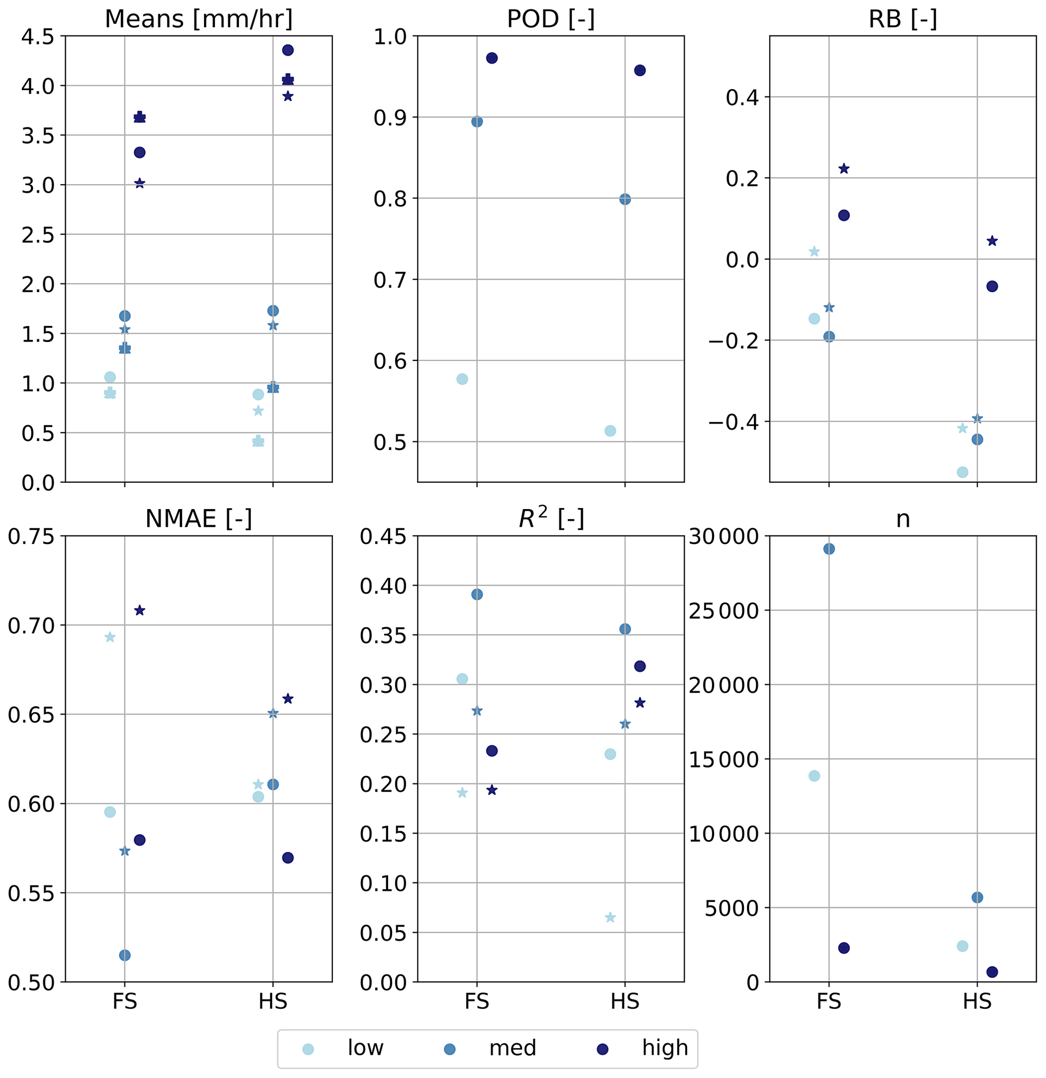
Figure 8Same as Fig. 2 but for the DPR. FS means “full scan” (both Ku-band and Ka-band over the entire Ku-band swath), HS represents “high-frequency scan” (observations from the Ka-band over the Ka-band swath, which is smaller than the Ku-band swath).
The effect of resampling is shown in Figs. 4–7. The difference in implementing either Gaussian weighting or uniform weighting is found to be negligible, especially for shallow observations. Hence, publications assuming circles or spatially averaged ellipses should yield comparable conclusions. Area is found to be the most important. Hence, it is expected that merging the different frequencies and sensors results in uncertainty added to the precipitation estimates of GPROF, as all observations are converted to GMI's 19 GHz footprint dimensions. Each sensor and frequency channel is associated with its own footprint, while GPROF assumes the footprint size associated with the 19 GHz channel.
Figure 6 illustrates that the sampling method has a limited effect on both the mean and standard deviation. Instead, they appear to be correlated with ETH, as expected, since higher ETH is often associated with more convection and higher precipitation rates. Additionally, ETH seems to be a better predictor of uncertainty in GPROF precipitation estimates, while the uncertainty related to sampling is minimal, as depicted in Figs. 2 and 3. Additionally, this discrepancy is largest for low ETH when the effect of footprint size is found to be minimal. Hence, improving the accuracy of shallow and light intensity precipitation estimates from spaceborne observations should be addressed by improving the (physical relations within) the algorithm. For instance, the DPR is used to match the radiometer observations to radar observations. This dependency can result in inaccuracies if the DPR is not able to capture shallow precipitation.
A brief evaluation of the DPR's performance is shown in Fig. 8. This figure clearly shows that the DPR has difficulties in both detecting and accurately quantifying the amount of shallow precipitation. However, as mentioned before, DPR observations are used to calibrate GPROF. Hence, future studies are recommended to focus more on the physical characteristics of shallow precipitation and how to improve their estimates using spaceborne sensors.
Radiometers are essential to provide global precipitation products based on uniformly distributed measurements from low-earth-orbit spatial platforms. Hence, a lot of effort is put into addressing persistent challenges and reducing uncertainties associated with algorithms that convert brightness temperatures into precipitation estimates. Yet, these algorithms will always be associated with some amount of uncertainty due to the merging of various channels with different footprint sizes for shallow and light precipitation as proven here over the Netherlands (53∘ N). This study provides insight into the magnitude of this uncertainty through resampling high-resolution estimates using different geometries and footprint sizes.
GPROF, the retrieval algorithm of the Global Precipitation Measurement mission (GPM) that converts brightness temperatures into precipitation estimates, was first evaluated to be able to quantify the discrepancy between space-based radiometer estimates and ground-based radar estimates. The R2 between GPROF and the reference varies between 0.23 and 0.37. Additionally, GPROF has difficulties to detect precipitation with a shallow vertical extent. As a next step, simulated footprints based on reference data used to evaluate GPROF were analyzed. This analysis provided insight into the uncertainties related to the combination of various channels, sensors, weighting methods, and their corresponding footprint dimensions.
The implemented weighting method and chosen geometry (circle or ellipse) were found to have a limited effect on the simulated footprints. Although the size of the footprints has a larger effect on the values of the retrieved estimates, it can not fully explain the discrepancies between GPROF and the reference estimates. Additionally, GPROF's relative bias is large for shallow ETH, while the relative bias between simulated estimates based on different sampling areas increases with ETH. We conclude that most of the uncertainty is related to the retrieval algorithm. At the same time, this study raises awareness about the inevitable uncertainties introduced when merging various channels and sensors. Hence, our results are also relevant for choosing appropriate footprint sizes when comparing to reference data.
All data from GPM can be accessed at https://gpm.nasa.gov/data/directory (Reed, 2023). The precipitation dataset can be retrieved using https://dataplatform.knmi.nl/dataset/rad-nl25-rac-mfbs-5min-netcdf4-2-0 (Overeem, 2023) and the echo top heights can be retrieved using https://dataplatform.knmi.nl/dataset/radar-tar-echotopheight-5min-1-0 (Leijnse, 2023).
LB: conceptualization, methodology, data, formal analysis, visualization and writing original draft. HL: conceptualization, methodology, supervision, and review. AO: conceptualization, methodology, supervision, and review. RU: conceptualization, methodology, supervision, and review.
The contact author has declared that none of the authors has any competing interests.
Publisher’s note: Copernicus Publications remains neutral with regard to jurisdictional claims made in the text, published maps, institutional affiliations, or any other geographical representation in this paper. While Copernicus Publications makes every effort to include appropriate place names, the final responsibility lies with the authors.
We would like to thank Claudia Brauer for her broader view on this paper and inspiring discussion on the figures. Furthermore, we would like to acknowledge Lisa Milani for sharing her expertise on shallow precipitation, in particular snowfall. We also thank the anonymous reviewer and Tom Rientjes for their constructive comments and suggestions.
This research has been supported by the Dutch Research Council (NWO, grant no. ALWGO.2018.048).
This paper was edited by Marloes Penning de Vries and reviewed by T.H.M. Rientjes and one anonymous referee.
Aberson, K.: The spatial and temporal variability of the vertical dimension of rainstorms and their relation with precipitation intensity, internal report, https://cdn.knmi.nl/knmi/pdf/bibliotheek/knmipubIR/IR2011-03.pdf (last access: 19 December 2023), 2011. a
Beekhuis, H. and Holleman, I.: Highlights of the digital-IF upgrade of the Dutch national radar network, online report, https://cdn.knmi.nl/system/data_center_publications/files/000/068/061/original/erad2008drup_0120.pdf?1495621011 (last access: 19 December 2023), 2008. a
Bogerd, L., Overeem, A., Leijnse, H., and Uijlenhoet, R.: A comprehensive five-year evaluation of IMERG late run precipitation estimates over the Netherlands, J. Hydrometeorol., 22, 1855–1868, https://doi.org/10.1175/JHM-D-21-0002.1, 2021. a, b
Casella, D., Panegrossi, G., Sanò, P., Milani, L., Petracca, M., and Dietrich, S.: A novel algorithm for detection of precipitation in tropical regions using PMW radiometers, Atmos. Meas. Tech., 8, 1217–1232, https://doi.org/10.5194/amt-8-1217-2015, 2015. a
Chang, N.-B. and Hong, Y.: Multiscale hydrologic remote sensing: perspectives and applications, CRC Press, ISBN 978-1-00-068727-9, 2012. a
Chen, F. and Li, X.: Evaluation of IMERG and TRMM 3B43 monthly precipitation products over mainland China, Remote Sens., 8, 472, https://doi.org/10.3390/rs8060472, 2016. a
Cristiano, E., ten Veldhuis, M.-C., and van de Giesen, N.: Spatial and temporal variability of rainfall and their effects on hydrological response in urban areas – a review, Hydrol. Earth Syst. Sci., 21, 3859–3878, https://doi.org/10.5194/hess-21-3859-2017, 2017. a
Ferraro, R. R., Peters-Lidard, C. D., Hernandez, C., Turk, F. J., Aires, F., Prigent, C., Lin, X., Boukabara, S.-A., Furuzawa, F. A., Gopalan, K., Harrison, K. W., Karbou, F., Li, L., Ringerud, S., Skofronick-Jackson, G. M., Tian, Y., and Wang, N.-Y.: An evaluation of microwave land surface emissivities over the continental United States to benefit GPM-era precipitation algorithms, IEEE Trans. Geosci. Remote, 51, 378–398, https://doi.org/10.1109/TGRS.2012.2199121, 2013. a
Foufoula-Georgiou, E., Ebtehaj, A. M., Zhang, S. Q., and Hou, A. Y.: Downscaling satellite precipitation with emphasis on extremes: a variational 1-norm regularization in the derivative domain, Surv. Geophys., 35, 765–783, https://doi.org/10.1007/s10712-013-9264-9, 2014. a
Guilloteau, C., Foufoula-Georgiou, E., and Kummerow, C. D.: Global multiscale evaluation of satellite passive microwave retrieval of precipitation during the TRMM and GPM eras: effective resolution and regional diagnostics for future algorithm development, J. Hydrometeorol., 18, 3051–3070, https://doi.org/10.1175/JHM-D-17-0087.1, 2017. a
Hayden, L. and Liu, C.: Differences in the diurnal variation of precipitation estimated by spaceborne radar, passive microwave radiometer, and IMERG, J. Geophys. Res.-Atmos., 126, e2020JD033020, https://doi.org/10.1029/2020JD033020, 2021. a
Hou, A. Y., Kakar, R. K., Neeck, S., Azarbarzin, A. A., Kummerow, C. D., Kojima, M., Oki, R., Nakamura, K., and Iguchi, T.: The Global Precipitation Measurement Mission, B. Am. Meteorol. Soc., 95, 701–722, https://doi.org/10.1175/BAMS-D-13-00164.1, 2014. a, b, c
Kidd, C. and Huffman, G.: Global precipitation measurement, Meteorol. Appl., 18, 334–353, https://doi.org/10.1002/met.284, 2011. a, b
Kidd, C. and Levizzani, V.: Chapter One – Quantitative precipitation estimation from satellite observations, in: Extreme Hydroclimatic Events and Multivariate Hazards in a Changing Environment, edited by: Maggioni, V. and Massari, C., 3–39, Elsevier, ISBN 978-0-12-814899-0, https://doi.org/10.1016/B978-0-12-814899-0.00001-8, 2019. a
Kidd, C., Tan, J., Kirstetter, P.-E., and Petersen, W. A.: Validation of the Version 05 Level 2 precipitation products from the GPM core observatory and constellation satellite sensors, Q. J. Roy. Meteorol. Soc., 144, 313–328, https://doi.org/10.1002/qj.3175, 2018. a
Kidd, C., Graham, E., Smyth, T., and Gill, M.: Assessing the impact of light/shallow precipitation retrievals from satellite-Based observations using surface radar and micro rain radar observations, Remote Sens., 13, 1708, https://doi.org/10.3390/rs13091708, 2021a. a
Kidd, C., Huffman, G., Maggioni, V., Chambon, P., and Oki, R.: The global satellite precipitation constellation: current status and future requirements, B. Am. Meteorol. Soc., 102, E1844–E1861, https://doi.org/10.1175/BAMS-D-20-0299.1, 2021b. a
Kim, K., Park, J., Baik, J., and Choi, M.: Evaluation of topographical and seasonal feature using GPM IMERG and TRMM 3B42 over Far-East Asia, Atmos. Res., 187, 95–105, https://doi.org/10.1016/j.atmosres.2016.12.007, 2017. a
Kubota, T., Ushio, T., Shige, S., Kida, S., Kachi, M., and Okamoto, K.: Verification of high-resolution satellite-based rainfall estimates around Japan using a gauge-calibrated ground-radar dataset, J. Meteorol. Soc. JPN II, 87A, 203–222, https://doi.org/10.2151/jmsj.87A.203, 2009. a
Kummerow, C., Hong, Y., Olson, W. S., Yang, S., Adler, R. F., McCollum, J., Ferraro, R., Petty, G., Shin, D.-B., and Wilheit, T. T.: The evolution of the Goddard profiling algorithm (GPROF) for rainfall estimation from passive microwave sensors, J. Appl. Meteorol. Climatol., 40, 1801–1820, https://doi.org/10.1175/1520-0450(2001)040<1801:TEOTGP>2.0.CO;2, 2001. a
Kummerow, C. D.: Introduction to passive microwave retrieval methods, in: Satellite Precipitation Measurement: Volume 1, edited by Levizzani, V., Kidd, C., Kirschbaum, D. B., Kummerow, C. D., Nakamura, K., and Turk, F. J., Advances in Global Change Research, 123–140 pp., Springer International Publishing, Cham, ISBN 978-3-030-24568-9, https://doi.org/10.1007/978-3-030-24568-9_7, 2020. a, b
Kummerow, C. D., Randel, D. L., Kulie, M., Wang, N.-Y., Ferraro, R., Joseph Munchak, S., and Petkovic, V.: The evolution of the Goddard profiling algorithm to a fully parametric scheme, J. Atmos. Ocean. Technol., 32, 2265–2280, https://doi.org/10.1175/JTECH-D-15-0039.1, 2015. a, b, c, d, e, f
Lee, Y.-R., Shin, D.-B., Kim, J.-H., and Park, H.-S.: Precipitation estimation over radar gap areas based on satellite and adjacent radar observations, Atmos. Meas. Tech., 8, 719–728, https://doi.org/10.5194/amt-8-719-2015, 2015. a
Leijnse, H.: Precipitation – radar 5 minute echo top height composites over the Netherlands, KNMI dataplatform [data set], https://dataplatform.knmi.nl/dataset/radar-tar-echotopheight-5min-1-0, last access: 19 December 2023. a
Leth, T. C. v., Leijnse, H., Overeem, A., and Uijlenhoet, R.: Rainfall spatiotemporal correlation and intermittency structure from micro-γ to meso-β scale in the Netherlands, J. Hydrometeorol., 22, 2227–2240, https://doi.org/10.1175/JHM-D-20-0311.1, 2021. a
Liu, C. and Zipser, E.: Differences between the surface precipitation estimates from the TRMM precipitation radar and passive microwave radiometer version 7 products, J. Hydrometeorol., 15, 2157–2175, https://doi.org/10.1175/JHM-D-14-0051.1, 2014. a
Lorenz, C. and Kunstmann, H.: The hydrological cycle in three state-of-the-art reanalyses: Intercomparison and performance analysis, J. Hydrometeorol., 13, 1397–1420, https://doi.org/10.1175/JHM-D-11-088.1, 2012. a
Maggioni, V., Meyers, P. C., and Robinson, M. D.: A review of merged high-resolution satellite precipitation product accuracy during the Tropical Rainfall Measuring Mission (TRMM) era, J. Hydrometeorol., 17, 1101–1117, https://doi.org/10.1175/JHM-D-15-0190.1, 2016. a, b, c
Maggioni, V., Massari, C., and Kidd, C.: Chapter 13 – Errors and uncertainties associated with quasiglobal satellite precipitation products, in: Precipitation Science, edited by: Michaelides, S., 377–390 pp., Elsevier, ISBN 978-0-12-822973-6, https://doi.org/10.1016/B978-0-12-822973-6.00023-8, 2022. a
McCollum, J. R. and Ferraro, R. R.: Microwave rainfall estimation over coasts, J. Atmos. Ocean. Technol., 22, 497–512, https://doi.org/10.1175/JTECH1732.1, 2005. a
Mega, T. and Shige, S.: Improvements of rain/no-rain classification methods for microwave radiometer over coasts by dynamic surface-type classification, J. Atmos. Ocean. Technol., 33, 1257–1270, https://doi.org/10.1175/JTECH-D-15-0127.1, 2016. a, b
Munchak, S. J. and Skofronick-Jackson, G.: Evaluation of precipitation detection over various surfaces from passive microwave imagers and sounders, Atmos. Res., 131, 81–94, https://doi.org/10.1016/j.atmosres.2012.10.011, 2013. a
O, S., Foelsche, U., Kirchengast, G., Fuchsberger, J., Tan, J., and Petersen, W. A.: Evaluation of GPM IMERG Early, Late, and Final rainfall estimates using WegenerNet gauge data in southeastern Austria, Hydrol. Earth Syst. Sci., 21, 6559–6572, https://doi.org/10.5194/hess-21-6559-2017, 2017. a
Overeem, A.: Precipitation – 5 minute precipitation accumulations from climatological gauge-adjusted radar dataset for The Netherlands, KNMI dataplatform [data set], https://dataplatform.knmi.nl/dataset/rad-nl25-rac-mfbs-5min-netcdf4-2-0, last access: 19 December 2023. a
Overeem, A., Buishand, T. A., and Holleman, I.: Extreme rainfall analysis and estimation of depth-duration-frequency curves using weather radar, Water Resour. Res., 45, https://doi.org/10.1029/2009WR007869, 2009a. a
Overeem, A., Holleman, I., and Buishand, A.: Derivation of a 10-year radar-based climatology of rainfall, J. Appl. Meteorol. Climatol., 48, 1448–1463, https://doi.org/10.1175/2009JAMC1954.1, 2009b. a
Overeem, A., Leijnse, H., and Uijlenhoet, R.: Measuring urban rainfall using microwave links from commercial cellular communication networks, Water Resour. Res., 47, W12505, https://doi.org/10.1029/2010WR010350, 2011. a
Passive Microwave Algorithm Team Facility: GPM GPROF Algorithm Theoretical Basis Document (ATBD), https://gpm.nasa.gov/sites/default/files/2022-06/ATBD_GPM_V7_GPROF.pdf (last access: 19 December 2023), 2022. a, b, c
Petty, G. W. and Bennartz, R.: Field-of-view characteristics and resolution matching for the Global Precipitation Measurement (GPM) Microwave Imager (GMI), Atmos. Meas. Tech., 10, 745–758, https://doi.org/10.5194/amt-10-745-2017, 2017. a
Pfreundschuh, S., Brown, P. J., Kummerow, C. D., Eriksson, P., and Norrestad, T.: GPROF-NN: a neural-network-based implementation of the Goddard Profiling Algorithm, Atmos. Meas. Tech., 15, 5033–5060, https://doi.org/10.5194/amt-15-5033-2022, 2022. a, b, c
Prigent, C.: Precipitation retrieval from space: an overview, Compt. Rendus Geosci., 342, 380–389, https://doi.org/10.1016/j.crte.2010.01.004, 2010. a
Randel, D. L., Kummerow, C. D., and Ringerud, S.: The Goddard Profiling (GPROF) precipitation retrieval algorithm, in: Satellite Precipitation Measurement: Volume 1, edited by: Levizzani, V., Kidd, C., Kirschbaum, D. B., Kummerow, C. D., Nakamura, K., and Turk, F. J., Advances in Global Change Research, 141–152 pp., Springer International Publishing, ISBN 978-3-030-24568-9, https://doi.org/10.1007/978-3-030-24568-9_8, 2020. a, b, c
Reed, J.: Precipitation Data Directory, NASA's Precipitation Processing Center [data set], https://gpm.nasa.gov/data/directory (last access: 19 December 2023), 2023. a
Saltikoff, E., Friedrich, K., Soderholm, J., Lengfeld, K., Nelson, B., Becker, A., Hollmann, R., Urban, B., Heistermann, M., and Tassone, C.: An overview of using weather radar for climatological studies: successes, challenges, and potential, B. Am. Meteorol. Soc., 100, 1739–1752, https://doi.org/10.1175/BAMS-D-18-0166.1, 2019. a
Shin, D.-B. and Kummerow, C.: Parametric rainfall retrieval algorithms for passive microwave radiometers, J. Appl. Meteorol. Climatol., 42, 1480–1496, https://doi.org/10.1175/1520-0450(2003)042<1480:PRRAFP>2.0.CO;2, 2003. a
Skofronick-Jackson, G., Petersen, W. A., Berg, W., Kidd, C., Stocker, E. F., Kirschbaum, D. B., Kakar, R., Braun, S. A., Huffman, G. J., Iguchi, T., Kirstetter, P. E., Kummerow, C., Meneghini, R., Oki, R., Olson, W. S., Takayabu, Y. N., Furukawa, K., and Wilheit, T.: The Global Precipitation Measurement (GPM) Mission for science and society, B. Am. Meteorol. Soc., 98, 1679–1695, https://doi.org/10.1175/BAMS-D-15-00306.1, 2017. a
Skofronick-Jackson, G., Berg, W., Kidd, C., Kirschbaum, D. B., Petersen, W. A., Huffman, G. J., and Takayabu, Y. N.: Global Precipitation Measurement (GPM): Unified precipitation estimation from space, in: Remote Sensing of Clouds and Precipitation, edited by: Andronache, C., Springer Remote Sensing/Photogrammetry, 175–193 pp., Springer International Publishing, Cham, ISBN 978-3-319-72583-3, https://doi.org/10.1007/978-3-319-72583-3_7, 2018a. a, b
Skofronick‐Jackson, G., Kirschbaum, D., Petersen, W., Huffman, G., Kidd, C., Stocker, E., and Kakar, R.: The Global Precipitation Measurement (GPM) mission's scientific achievements and societal contributions: reviewing four years of advanced rain and snow observations, Q. J. Roy. Meteorol. Soc., 144, 27–48, https://doi.org/10.1002/qj.3313, 2018b. a
Stephens, G. L. and Kummerow, C. D.: The remote sensing of clouds and precipitation from space: A review, J. Atmos. Sci., 64, 3742–3765, https://doi.org/10.1175/2006JAS2375.1, 2007. a
Sun, Q., Miao, C., Duan, Q., Ashouri, H., Sorooshian, S., and Hsu, K.-L.: A Review of Global Precipitation Data Sets: Data Sources, Estimation, and Intercomparisons, Rev. Geophys., 56, 79–107, https://doi.org/10.1002/2017RG000574, 2018. a
Tan, J., Cho, N., Oreopoulos, L., and Kirstetter, P.: Evaluation of GPROF V05 precipitation retrievals under different cloud regimes, J. Hydrometeorol., 23, 389–402, https://doi.org/10.1175/JHM-D-21-0154.1, 2022. a, b
Tang, G., Clark, M. P., Papalexiou, S. M., Ma, Z., and Hong, Y.: Have satellite precipitation products improved over last two decades? A comprehensive comparison of GPM IMERG with nine satellite and reanalysis datasets, Remote Sens. Environ., 240, 111697, https://doi.org/10.1016/j.rse.2020.111697, 2020. a
Wang, Y., You, Y., and Kulie, M.: Global virga precipitation distribution derived from three spaceborne radars and its contribution to the false radiometer precipitation detection, Geophys. Res. Lett., 45, 4446–4455, https://doi.org/10.1029/2018GL077891, 2018. a
You, Y., Peters-Lidard, C., Turk, J., Ringerud, S., and Yang, S.: Improving overland precipitation retrieval with brightness temperature temporal variation, J. Hydrometeorol., 18, 2355–2383, https://doi.org/10.1175/JHM-D-17-0050.1, 2017. a
You, Y., Petkovic, V., Tan, J., Kroodsma, R., Berg, W., Kidd, C., and Peters-Lidard, C.: Evaluation of V05 precipitation estimates from GPM constellation radiometers using KuPR as the reference, J. Hydrometeorol., 21, 705–728, https://doi.org/10.1175/JHM-D-19-0144.1, 2020. a, b