Cloud optical and physical properties retrieval from EarthCARE multi-spectral imager: the M-COP products

The Earth Cloud, Aerosol and Radiation Explorer (EarthCARE) is the first mission that will provide measurements from active profiling, passive imaging and a broadband radiometer from a single satellite platform. The passive multi-spectral imager (MSI) features four solar and three thermal infrared channels, and has a swath of 150 km and a spatial pixel resolution of 500 m. The MSI observations will provide across-track information on clouds and aerosol to extend the active profiling information into the swath. In this paper, we present the algorithm used for retrieving the cloud optical and physical products (M-COP), specifically cloud optical thickness, effective radius and top height. The algorithm is based on the solar and terrestrial MSI channels within an optimal estimation framework. This framework enables full error propagation given by the uncertainties in measurements and a priori information. The MSI cloud algorithm has been successfully exercised on different imagers and on synthetically generated MSI observations.

1 Introduction

Clouds play an important role in the earth's radiation budget due to their strong interaction with atmospheric radiation and the resulting complex influence on radiative fluxes (Hartmann and Short, 1980). Global-scale satellite observations of clouds and radiation are thus essential for our knowledge about the earth's energy budget and climate system. Of particular interest are cloud changes in response to anthropogenic influences, including aerosol emissions, which manifest as radiative forcing and can potentially contribute to a number of feedback processes and thus further amplify climate change (, ).

There is an urgent need for long-term, high-quality global-scale observations to improve our understanding of cloud processes including their representation in weather and climate models. Here, the interaction of aerosol particles and clouds deserves particular focus, due to the uncertainty introduced in climate change projects.

Since the early 1980s, a number of satellite missions have provided multi-spectral imagery as a basis for long-term global-scale cloud and radiation datasets. A particularly noteworthy effort is the International Satellite Cloud Climatology Project (ISCCP), which utilized both the early geostationary satellite instruments and the advanced very high resolution radiometer (AVHRR) flown on NOAA's operational polar-orbiting satellite series. The intercalibration of individual sensors to yield a homogeneous record was found to deserve special attention for data consistency. Over time, the observational capabilities of these passive imaging spectrometers have also greatly improved for the polar-orbiting Moderate-Resolution Imaging Spectrometer (MODIS), the Visible Infrared Imaging Radiometer Suite (VIIRS) and geostationary satellites (e.g. Geostationary Operational Environmental Satellites (GOES), Meteosat Second Generation (MSG) and Himawari).

A variety of methods and datasets exist for the determination of cloud microphysical properties from multi-spectral satellite imagery, for example, from AVHRR (Derrien et al., 1993; Kriebel et al., 1989; Nakajima and King, 1990; Walther and Heidinger, 2012), the Along-Track Scanning Radiometer (ATSR; Watts et al., 1998), MODIS (King et al., 1997; Platnick et al., 2017), VIIRS (Platnick et al., 2021), the Advanced Himawari Imager (AHI; Letu et al., 2020), the GOES series (Minnis and Harrison, 1984; Heidinger et al., 2020) and the Spinning Enhanced Visible and Infrared Imager (SEVIRI; Stengel et al., 2014). All these methods share a fundamental principle: the reflection of clouds in the visible and near infrared wavelength region, specifically in a non-absorbing channel, is primarily determined by cloud optical thickness. In contrast, the reflection function at absorbing channels in the shortwave infrared region strongly depends on cloud particle size. Hence, at present, there are several long-term, consistent satellite-based climate data records of cloud properties available from passive satellite imagery, with various differences in time coverage, accuracy and availability of parameters, which ultimately determines their suitability for a particular scientific question (Stubenrauch et al., 2013).

Passive multi-spectral satellite imagers have inherent limitations in terms of their information content, providing only indirect and limited details about cloud vertical structure. However, a significant breakthrough occurred with the launch of CloudSat and CALIPSO (Cloud and Aerosol Lidar and Infrared Pathfinder Mission) satellites in 2006, which joined the A-Train satellite constellation. These satellites introduced a novel perspective from space by providing unprecedented and detailed information on the intricate vertical structure of cloud and aerosol profiles. The CloudSat satellite incorporated the Cloud Profiling Radar (CPR), while CALIPSO carried the CALIOP (Cloud and Aerosol Lidar with Orthogonal Polarization) instruments. These instruments marked the first long-term active remote sensing observations from space (Stephens and Kummerow, 2007).

The EarthCARE satellite mission is a joint mission by the European and Japanese space agencies, and is the European Space Agency's (ESA) sixth Earth Explorer. The spacecraft will feature four instruments on a single platform: the cloud profiling Radar (CPR) with Doppler capability, the high spectral resolution atmospheric lidar (ATLID), the multi-spectral imager (MSI), and the broadband radiometer (BBR) (Wehr et al., 2023). The satellite measurements will be used to retrieve global profiles of cloud, aerosol, and precipitation properties, along with top of atmosphere terrestrial and solar fluxes (Illingworth et al., 2015). The MSI instrument measures in seven channels in the visible, near infrared, shortwave infrared and infrared spectrum, with central wavelengths of 0.67 (VIS), 0.865 (NIR), 1.65 (SWIR1), 2.21 (SWIR2), 8.8 (TIR1), 10.8 (TIR2), and 12.0 µm (TIR3), and with 500 m spatial resolution (Wehr et al., 2023). MSI will have a swath width of 150 km, asymmetrically tilted away from the sun and covering 35 km to the west side and 115 km to the east side of the nadir. MSI observations will be used to provide cloud products and to extend the spatially limited coverage of cloud properties obtained from the active sensors into the across-track direction. Furthermore, the information gained from the MSI swath will make it possible to identify weather phenomena at the mesoscale or even synoptic scale, and utilize these as context for the interpretation of the active observations. The cloud microphysical retrievals are based on the combination of the non-absorbing visible channels and the absorbing shortwave infrared channels. MSI has no dedicated absorption channels for cloud top determination. Therefore, the cloud top height retrieval is limited to the information from the infrared window channels (Inoue, 1985; Fritz and Winston, 1962). To compensate for the instrument limitations and ensure consistency between the products, the cloud microphysical retrieval is combined with the macrophysical retrievals into one retrieval algorithm similar to that of Watts et al. (2011) or Poulsen et al. (2012).

The goal of the present paper is to introduce the algorithms used as a basis for the cloud property retrievals, which will be applied operationally to MSI observations as part of the MSI cloud processor (M-CLD; Fig. A1). The M-CLD consists of two main parts, which are sequentially processed. First the cloud mask (M-CM) is processed with output of the cloud flag (M-CF) and cloud phase (M-CP) product (Hünerbein et al., 2023), which are mandatory to retrieve the cloud optical and physical product (M-COP). The M-COP includes the cloud optical thickness (M-COT), cloud effective radius (M-REF), cloud top temperature/height/pressure (M-CTT, M-CTH, M-CTP), and the cloud water path (M-CWP) for daylight conditions. During nighttime, only the cloud top temperature/height/pressure can be provided. The instrumental characteristics of the MSI sensor, which largely determine the design and accuracy of the M-COP retrievals, are described in more detail in Wehr et al. (2023).

This paper is structured as follows: in Sect. 2, the operational level 2 M-COP algorithms are described in detail. Section 3 presents some examples of the verification of the M-COP products. This has been performed by applying the M-CLD processor to the EarthCARE simulator test scenes (Donovan et al., 2023), MODIS measurements and SEVIRI measurements. Finally, the results are summarized and discussed in Sect. 4.

2 M-COP algorithm description

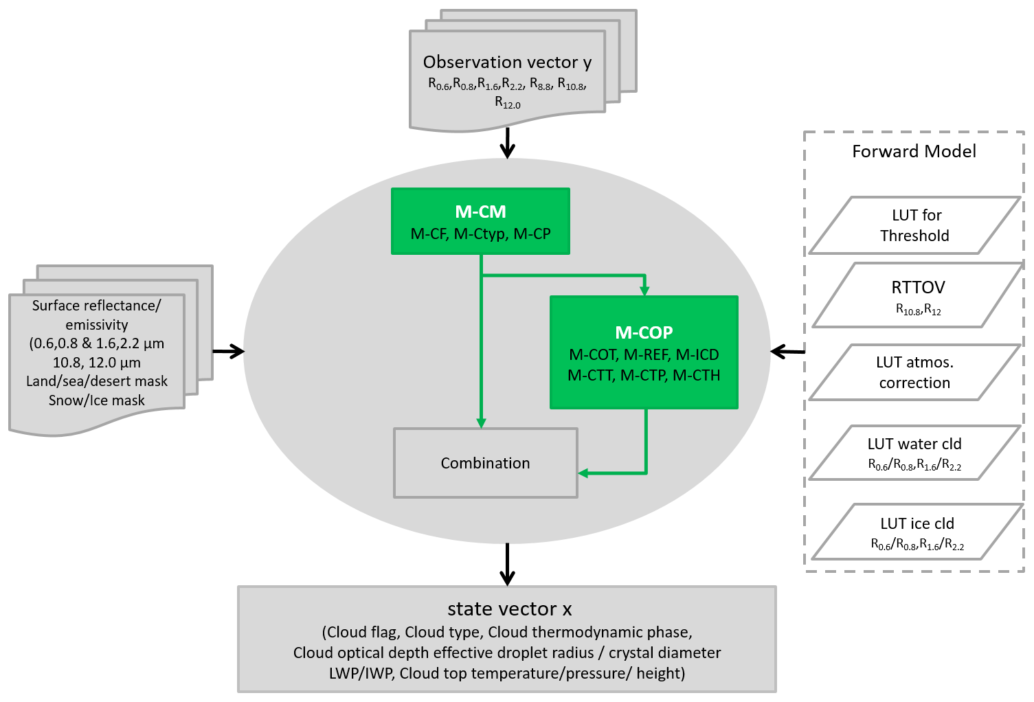
The M-COP retrieval uses multiple MSI channels in visible and shortwave infrared and thermal range of the electromagnetic spectrum to derive cloud optical thickness (M-COT), effective cloud radius (M-REF) and multiple estimates of cloud height (M-CTT, M-CTH and M-CTP) as output products. The algorithm is embedded in the M-CLD processor framework. While it is in many aspects similar to already existing cloud retrievals for current sensors in space (e.g. MODIS and SEVIRI), it has been implemented from scratch following a mathematically optimal estimation approach. An overview of the workflow is given in Fig. 1. The main idea is to compare simulated reflectance and radiance values for a wide range of possible atmospheric conditions with the measured values from the sensor. The simulations, which build the forward model of the retrieval, are partly created in advance with a radiative transfer model (RTM) and then stored in look-up tables. We decided to use an optimal estimation (OE) inversion technique (Sect. 2.4) (Rodgers, 2000), because this provides very nicely an uncertainty propagation from the measurement through the forward model to product uncertainty estimates. M-COP assumes cloud mask and cloud phase as a known input. These parameters are supplied from directly preceding procedures within the M-CLD processor (Hünerbein et al., 2023). Furthermore, background information on the atmospheric and surface states, such as humidity and temperature profiles and surface reflectance and emissivity, is needed. We get this information from the auxiliary meteorological database (X-MET; Eisinger et al., 2023), which is specifically initiated for this mission. The OE technique finds the best estimate of the cloud properties by an iterative retrieval loop, which compares the forward model result of an assumed state vector with the observation by taking into account the respective uncertainties. Once the forward model output of the assumed state vector and the observation vector satisfy the requirement of the minimization of a cost function, the retrieval process is considered successful. This state vector then represents the solution. We present in the following subsections details of the components of M-COP.

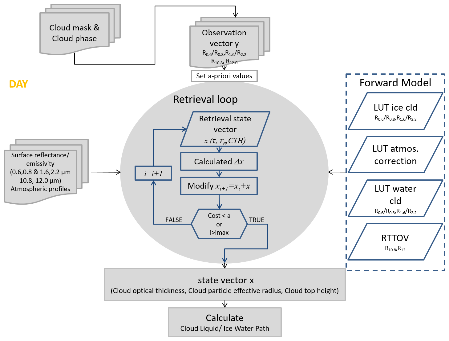
Figure 1 Flowchart of the M-COP algorithm. The algorithm is applied to all cloudy MSI pixels.

2.1 Input data

The MSI L1c products are calibrated and geolocated instrument data. The measurements for solar channels are given in radiance and the three terrestrial channels in brightness temperature. The L1c product is re-sampled onto the grid of a reference TIR channel (Eisinger et al., 2023). Therefore, each channel is mapped on the same pixel, which is important for the M-CLD processor, where we use the combination of all channels. The algorithm starts with the calculation of the reflectances at the top of the atmosphere in the solar channels. The reflectances $R({\mathit{\theta }}_{\mathrm{0}},\mathit{\theta },\mathit{\varphi })$ of each channel i are obtained from the following input parameters: the measured radiance (L) and the corresponding inband solar irradiance E₀,i as $R({\mathit{\theta }}_{\mathrm{0}},\mathit{\theta },\mathit{\varphi })$ = $\frac{\mathit{\pi }{L}_i({\mathit{\theta }}_{\mathrm{0}},\mathit{\theta },\mathit{\varphi })}{E_{\mathrm{0}},icos\left({\mathit{\theta }}_{\mathrm{0}}\right)}$ and i= VIS, NIR, SWIR1, SWIR2. The measured radiance and brightness temperature for each pixel depends on the solar zenith angle θ₀, the viewing zenith angle θ and the relative azimuth angle ϕ, defined by the difference between the sun and instrument viewing azimuth angles.

2.2 Ancillary data

The retrieval requires further background information on atmospheric and surface conditions. The forward model includes a reflectance term which accounts for backscattered radiation from the underlying surface. For land pixels, we use the long-term albedo climatology from the MODIS science team (Moody et al., 2008). We assume that the white-sky albedo product is best suited for cloudy atmospheres since it refers to the reflection of incoming diffuse radiation. MODIS has very similar channel specifications so that these data can be used as they are. Over ocean, the surface albedo is assumed to be 0.05 at both 0.6 and 1.6 µm. For the forward model in the longwave channels, we use the land surface emissivity values provided by the MODIS land surface temperature and emissivity products, which provide per-grid temperature and emissivity values (Wan, 2014).

2.3 Forward model

The forward model is an operator that simulates the observed radiance at the sensor based on a known atmospheric state and given auxiliary input parameters. It is strictly channel based, such that the complete operator is composed of independent simulations of the channel i from a set of

$$F_i\left(x\right)=y,$$

where x is the state vector of the atmosphere (including the cloud properties) and y the vector of the observations (the measurements). The forward operator F includes the auxiliary data with their uncertainties. The individual components of the equation are separated into the solar spectrum with negligible terrestrial emission (up to 3.5 µ wavelength) and the part of the spectrum where thermal emission dominates the radiative transfer.

Segelstein (1981)Warren and Brandt (2008)

Table 1 Summary of the setup for generating the M-COP LUTs for VIS and SWIR1 channels.

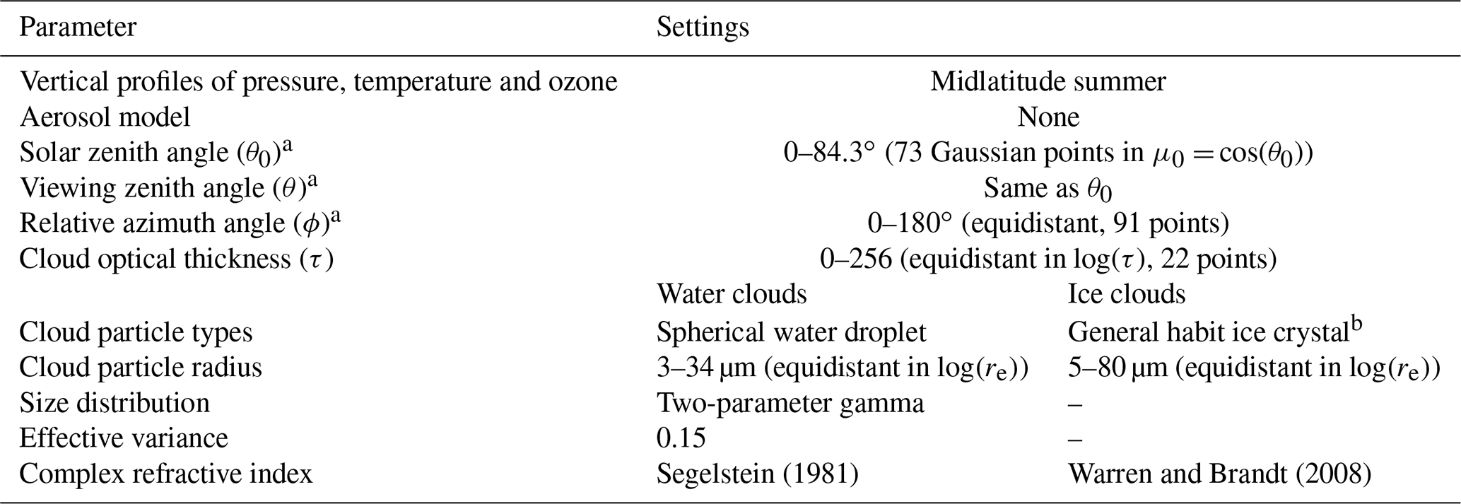
^a The chosen distributions of angles are from Wolters et al. (2006). ^b From Baum et al. (2014).

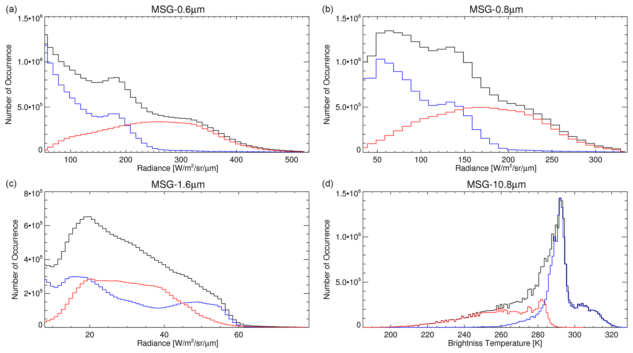
Figure 2 Histogram of the radiance in VIS, NIR, SWIR-1 and the brightness temperature TIR-2 based on SEVIRI measurements for cloud free (blue), cloudy (red) and mixed (black) cases.

2.3.1 Visible and shortwave infrared radiative transfer

This part of the forward model is built on an existing retrieval algorithm, the Cloud Physical Properties (CPP; Roebeling et al., 2006), which was developed at The Royal Netherlands Meteorological Institute (KNMI) and has been used operationally for SEVIRI and AVHRR for more than a decade. It has been validated and improved over the years (Greuell and Roebeling, 2009; Roebeling et al., 2013; Benas et al., 2017).

Radiative transfer in this range is formulated in terms of reflectance values. The measured spectral reflectance R_toa at the top of the atmosphere can be expressed for a known surface reflectance α_s and a known geometrical constellation as

$$\begin{array}{}\text{(1)}& \begin{array}{rl}{R}_{\mathrm{toa}}& (\mathit{\tau },r_{\mathrm{e}},{\mathit{\theta }}_{\mathrm{0}},\mathit{\theta },\mathit{\varphi })=R_{\mathrm{cl}}(\mathit{\tau },r_{\mathrm{e}},{\mathit{\theta }}_{\mathrm{0}},\mathit{\theta },\mathit{\varphi })\\ & +{\displaystyle \frac{{\mathit{\alpha }}_s{t}_{\mathrm{c}}(\mathit{\tau },r_{\mathrm{e}},{\mathit{\theta }}_{\mathrm{0}})t_{\mathrm{c}}(\mathit{\tau },r_{\mathrm{e}},\mathit{\theta })}{\mathrm{1}-{\mathit{\alpha }}_s{\mathit{\alpha }}_{\mathrm{a}}(\mathit{\tau },R_{\mathrm{e}})}},\end{array}\end{array}$$

where τ is the cloud optical thickness, r_e the effective radius of cloud particle distribution, α the surface reflectance, t_c cloud transmittance (which is needed for both angles, incoming θ₀ and outgoing θ), R_cl the cloud reflectance and α_a the hemispherical sky albedo for upwelling, isotropic radiation (also known as spherical albedo). Other effects below and above the cloud layer are neglected in this equation. The aim is to find the pair of τ,r_e which gives the highest accordance, or even better, the optimal estimate for the set of equations above for the VIS/SWIR1 channels. Within the retrieval loop, a pair of τ,r_e is assumed initially (i.e. a priori) and the result R_toa of the forward model is compared with the observations to adjust the assumption till an optimal result is found. Thus, the functions R_cl, t_c and α_a have to be simulated during the retrieval loop. Since this is not a simple and fast task, it is carried out in advance, and the results are stored in look-up tables (LUT) and interpolated from there to speed up the processing.

Table 2 Comparison of the minimum and maximum radiances and brightness temperatures from the SEVIRI channels.

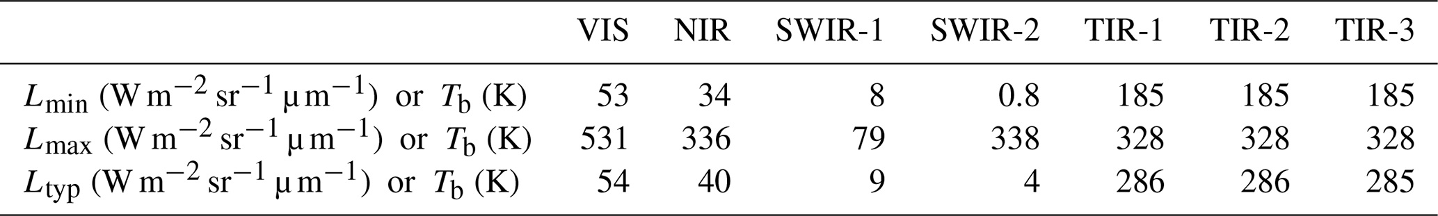
Table 3 Geophysical variable error used based on the breakthrough values of the user requirement tables from the position paper (Rizzi et al., 2006).

To generate these tables we use the radiative transfer model, DAK (Doubling-Adding KNMI; de Haan et al., 1987; Stammes, 2001). To take into account also the Rayleigh scattering and ozone absorption above a cloud, the simulations were carried out with standard atmospheric states. Table 1 summarizes the LUT settings together with binning of individual dimensions. DAK can simulate cloud reflectance, cloud transmittance and cloud spherical albedo without the influence of surface reflectivity, such that the second term on the right side of Eq. (1) takes this into account directly during the optimization process.

The DAK calculations concern monochromatic radiative transfer at a wavelength close to the centre of the respective satellite channel. This implies an assumption that reflectance at the central wavelength is close enough to the average reflectance over the channel. The radiative transfer calculations neglect scattering and absorption by atmospheric gases, except for Rayleigh scattering by air molecules and absorption by ozone.

The atmospheric correction for scattering and absorption processed in layers above cloud top is derived by the MODTRAN radiative transfer model Berk et al. (2000). The atmosphere corrected top of atmosphere reflectance ($R_{\mathrm{atm}.\mathrm{corr}.}$) is calculated as

$$\begin{array}{}\text{(2)}& R_{\mathrm{atm}.\mathrm{corr}.}=R_{\mathrm{toa}}{t}_{\mathrm{a},\mathrm{ac}}({\mathit{\theta }}_{\mathrm{0}},z_{\mathrm{ct}},H)t_{\mathrm{a},\mathrm{ac}}(\mathit{\theta },z_{\mathrm{ct}},H,\mathrm{TCO}),\end{array}$$

where t_a,ac is the above-cloud atmospheric transmission simulated by MODTRAN using a Lambertian surface placed at the cloud top height (z_ct, M-CTH) and for a given water vapour path (H, humidity profile) and total column ozone (TCO). The two-way transmission, i.e. the product of the two transmission values, is a function of the geometrical air mass factor ($\mathrm{AMF}=\mathrm{1}{/}_{\mathrm{0}}+\mathrm{1}/$). This two-way transmission is calculated in advance for a wide range of AMFs and stored in an LUT with dimensions AMF, z_ct and H. Absorption by trace gases within and below the cloud is neglected. More details on the implementation of atmospheric correction and the effect on retrieved cloud properties can be found in Meirink et al. (2009).

2.3.2 Terrestrial radiative transfer

In contrast to the solar forward model, the thermal part includes mainly the emission from surface, atmosphere and cloud layers. The calculations are done with RTTOV 11.3 Saunders et al. (2009, 1999). The forward simulations of the infrared radiances are used to compare the observed MSI brightness temperature with the simulated brightness temperature to retrieve the M-CTT based on the method of Fritz and Winston (1962). The simulations require atmospheric profiles, e.g. temperature (T) and humidity (H), which are provided by the X-MET product (Eisinger et al., 2023). The top of the atmosphere radiance (L) or brightness temperature (T_b) at 8.8, 10.8 and 12.0 µm will be simulated once for clear sky and black cloud (emissivity equal 1) conditions. The overcast radiance (L) consists of contributions from four terms, i.e. transmission radiance upwelling from below cloud level (L_s), emission from the cloud (L_c), reflection of radiance downwelling from above the cloud level and emission of radiance from the atmosphere above the cloud (L_at):

$$\begin{array}{}\text{(3)}& L(x,\mathit{\theta },\mathit{ϵ})=L_{\mathrm{s}}+L_{\mathrm{c}}+L_{\mathrm{at}}.\end{array}$$

The surface partition can be formulated with

$$\begin{array}{}\text{(4)}& L_{\mathrm{s}}(x,\mathit{\theta },{\mathit{ϵ}}_{\mathrm{s}})={\mathit{ϵ}}_{\mathrm{s}}B\left(T_{\mathrm{s}}\right)t_{\mathrm{a}}\left(\mathit{\theta }\right)t_{\mathrm{c}}\left(\mathit{\theta }\right),\end{array}$$

and is a function of surface emissivity ϵ_s and the Planck function of surface temperature. Both values are assumed as known from the X-MET dataset. $t_{\mathrm{c}}=\mathrm{1}-{\mathit{ϵ}}_{\mathrm{c}}$; for optically very thick clouds the cloud emissivity is equal to 1. In this case the surface as well as the atmospheric layer below the cloud is not contributing to the TOA (top of the atmosphere) radiance. t_a is the transmission of the atmosphere. The cloud part of Eq. (3) is formulated as

$$\begin{array}{}\text{(5)}& L_{\mathrm{c}}(x,\mathit{\theta },{\mathit{ϵ}}_{\mathrm{c}})={\mathit{ϵ}}_{\mathrm{c}}(\mathit{\tau },\mathit{\theta })B\left(T_{\mathrm{c}}\right)t_{\mathrm{ac}}\left(\mathit{\theta }\right),\end{array}$$

where we again have to assume the emissivity of the cloud layer, and the cloud top temperature. The cloud emissivity can be parameterized by ${\mathit{ϵ}}_{\mathrm{c}}=\mathrm{1}-\exp [-{\mathit{\tau }}_{\mathrm{ir}}/\cos \mathit{\theta }]$ by assuming the optical thickness in IR range with τ_ir=0.5τ_vis (Minnis et al., 1993).

The value t_a depicts the entire atmospheric transmission from cloud top to the top of the atmosphere. The radiance coming from atmospheric layers outside the cloud is simulated with RTTOV 11.3 for different atmospheric levels z based on auxiliary data $(T,P,H)$ profiles:

$$\begin{array}{}\text{(6)}& L_{\mathrm{at}}(\mathit{\theta },{\mathit{ϵ}}_{\mathrm{s}})=\underset{t_{\mathrm{s}}}{\overset{\mathrm{1}}{\int }}B\left(T_{\mathrm{a}}\right)\mathrm{d}t+[\mathrm{1}-{\mathit{ϵ}}_{\mathrm{s}}]*t_{\mathrm{s}}(\mathit{\theta }{)}^{\mathrm{2}}\underset{t_{\mathrm{s}}}{\overset{\mathrm{1}}{\int }}{\displaystyle \frac{B\left(T_{\mathrm{a}}\right)}{t(\mathit{\theta }{)}^{\mathrm{2}}}}\mathrm{d}t,\end{array}$$

whereby t_s is the total transmission from the surface to the top of the atmosphere.

Note that we can modulate the cloud emissivity by changing the cloud optical thickness and the cloud top height as an input parameter.

Table 4 Minimum and maximum values of the state vector.

2.4 Retrieval Method

The retrieval loop (Fig. 1) uses 1D-var optimal estimation inversion techniques to retrieve the cloud optical thickness, effective radius and cloud top heights during daytime, which is defined by the solar zenith angle (θ<84^∘). At nighttime the retrieval relies on the infrared channels and only the cloud top height is retrieved.

2.4.1 Optimal estimation

The basic principle of the M-COP algorithm follows the description of Rodgers (2000). The OE method is commonly used to solve the inverse problem (e.g. Watts et al., 2011; Walther and Heidinger, 2012; Poulsen et al., 2012). The OE does not provide an explicit solution but rather a class of solutions and assigns a probability density to each. The probability P(x|y) of the retrieval state for all possible solutions x for a given observation y is defined as $P\left(\mathit{x}\mathbf{\right|}\mathit{y})=\frac{P\left(\mathit{y}\mathbf{\right|}\mathit{x}\left)P\right(\mathit{x})}{P\left(\mathit{y}\right)}$

• P(x): prior PDF of the atmospheric state x

• P(y|x): conditional PDF of y given x; requires knowledge of the forward model and statistical description of the measurement error

• P(y): prior PDF of the measurement y.

The solution is found by maximizing the probability P(x|y) related to the values of the state vector x. The a priori estimate of the state is defined by x_a and the measurement vector y is defined as a three element vector with visible, shortwave IR and infrared radiances:

$$\mathit{x}=\left(\begin{array}{c}\mathit{\tau }\\ r_{\mathrm{e}}\\ \mathrm{CTT}\end{array}\right)\text{and}\mathit{y}=\left(\begin{array}{c}{R}_{\mathrm{vis}}\\ R_{\mathrm{swir}\mathrm{1}}\\ T_{\mathrm{b}}\end{array}\right).$$

The state is mapped into the measurement space with the forward model F(x) (see Sects. 2.3.1 and 2.3.2). The OE is based on the assumption that the errors in the measurements S_e and background S_a can be described by a Gaussian distribution. Therefore, the state vector x should be preferable and also Gaussian distributed. To account for this, the τ and r_e are transformed in the logarithmic space with a base two for the inversion, which leads also to a more Gaussian error distribution. In order to find the solution, an iterative search is done by maximizing P(x|y) or minimize the cost function J, which comprises the measurement error and the background knowledge:

$$J\left(\mathit{x}\right)=\left(F\right(\mathit{x})-\mathit{y}){\mathbf{S}}_{\mathrm{e}}^{-\mathrm{1}}\left(F\right(\mathit{x})-\mathit{y}{)}^T+(\mathit{x}-{\mathit{x}}_{\mathrm{a}}\left){\mathbf{S}}_{\mathrm{a}}^{-\mathrm{1}}\right(\mathit{x}-{\mathit{x}}_{\mathrm{a}}{)}^T).$$

The M-COP retrieval loop starts with defined a priori values for the state vector x and the observation y. The cost J is calculated for each iteration step. Each iteration step of the retrieval loop requires search events in the forward model operators F. The derived radiances by the forward model F(x_i) are compared with measurement, y which defines the cost function. The optimal estimation searches for the minima in the cost function until convergence. The Levenberg–Marquardt descent method is used for the minimization within an iteration process (Marquardt, 1963; Levenberg, 1944). If the cost reaches a pre-defined threshold, the solution is found and the retrieval loop will end.

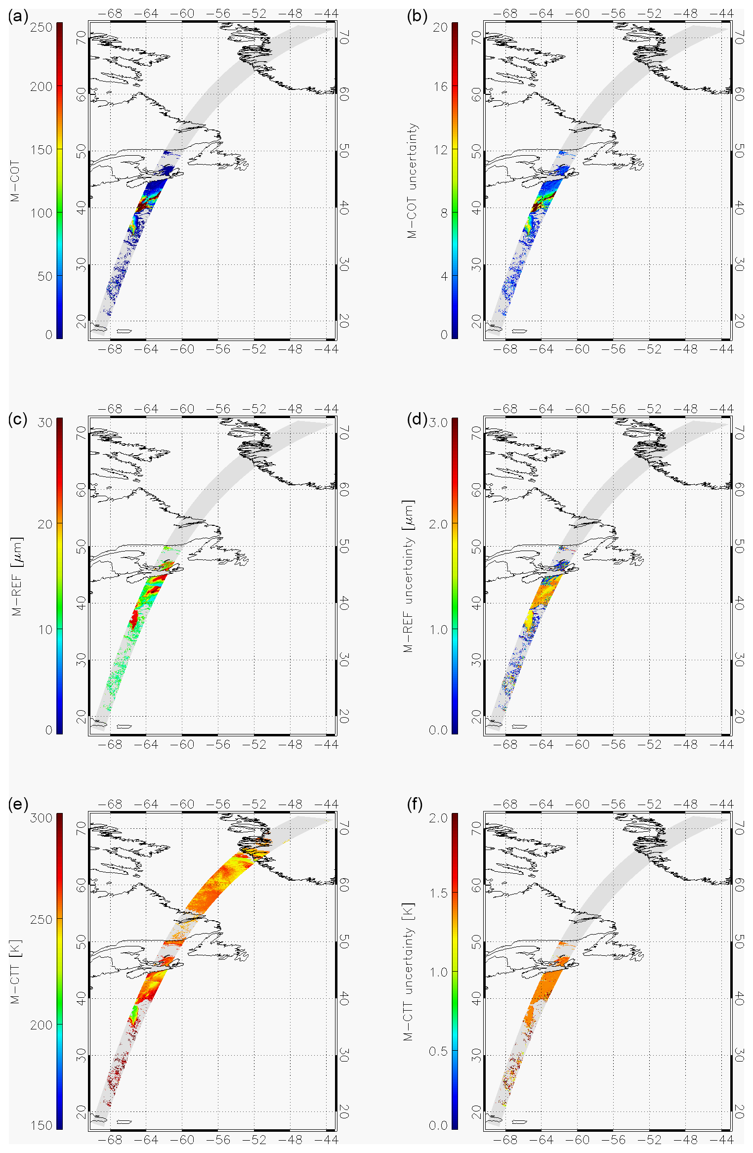
Figure 3 M-COP for the HALIFAX scene with M-COT (a), OE uncertainties of M-COT (b), M-REF (c), OE uncertainties of M-REF (d), CTT (e) and OE uncertainties of CTT (f). Note that for nighttime CTT retrieval no uncertainty is provided.

2.4.2 Measurement vector and covariance matrix

A global set of SEVIRI data have been studied in order to establish typical top of the atmosphere radiances and brightness temperatures. The SEVIRI instrument aboard MSG (Meteosat Second Generation) offers excellent measurements to study the global variation of the radiances. SEVIRI covers the visible (VIS006, VIS008), the near infrared (NIR016) and the thermal infrared spectral region (IR039, IR062, IR073, IR087, IR097, IR108, IR120 and IR134) with 12 channels. These SEVIRI channels match the spectral position of the same MSI channels. This gives us the possibility to use the SEVIRI dataset for comparison of the maximum and minimum radiances, as well as for the specification of the typical radiance. To get the full range of the four seasons the criteria for the dataset were time: 09:00 UTC; day: in the mid of the months; month: March, June, September, December; year: 2007; for all SEVIRI pixels.

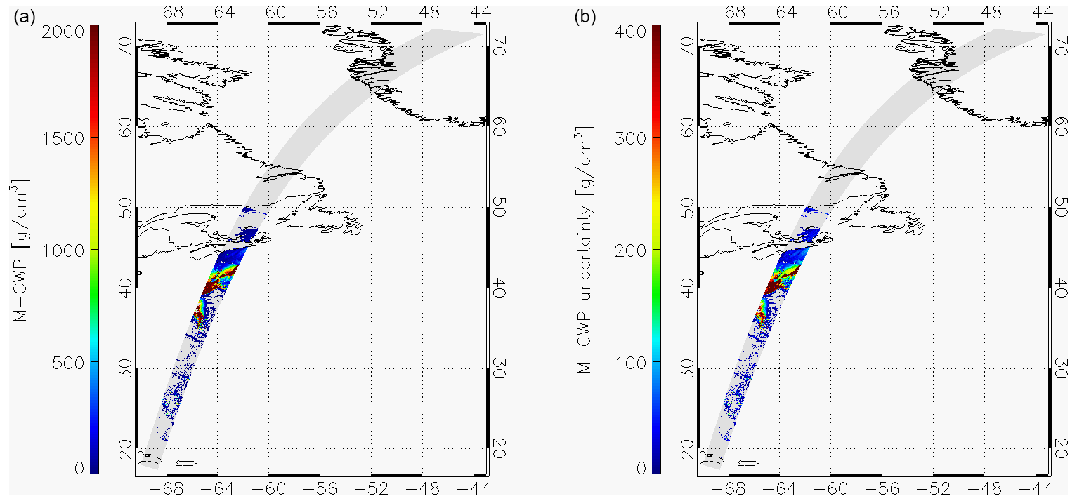
Figure 4 M-CWP of the HALIFAX scene (a) and the OE uncertainties of M-CWP (b).

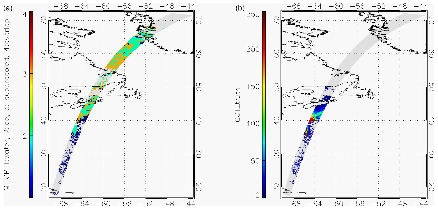
Figure 5 M-CP of the HALIFAX scene (a) and the true cloud optical thickness at 680 nm (b).

The histogram distributions for cloudy, clear and mixed cases have been studied (see Fig. 2), and the maximum and minimum radiances and brightness temperatures have been taken from cloud free and cloudy atmosphere. From the mixed cases the typical scene radiances were estimated from the 50th percentile of the data. The typical radiances of the MSI channels are specified with the comparable SEVIRI channels (see Table  2).

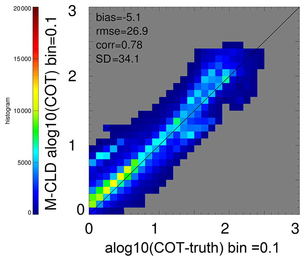
Figure 6 Histogram of the true cloud optical thickness and M-COT for the Halifax scene histogram.

The measurement and background knowledge are described by the covariance matrices. The measurement error S_e is defined through the instrument signal-to-noise ratio or the noise equivalent different temperature (Wehr et al., 2023) and the forward model error as

$${\mathbf{S}}_{\mathrm{e}}={\left({\displaystyle \frac{L_{\mathrm{typ}}}{\mathrm{SNR}}}\right)}^{\mathrm{2}}+\sum _n({\mathbf{K}}_n\mathit{a}\mathit{c}{\mathit{c}}_n{)}^{\mathrm{2}},n=\mathit{\tau },r_{\mathrm{e}},\mathrm{CTT}.$$

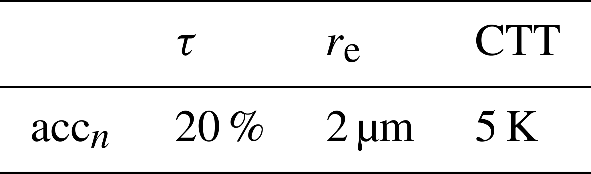
The typical radiances L_typ are taken from the above described SEVIRI analysis. This will be adapted during the commissioning phase to on-board measured uncertainties and radiances. The forward model errors are calculated by the Jacobians K and the geophysical variable error acc_n for each iteration step. The applied geophysical variable errors are provided in Table 3.

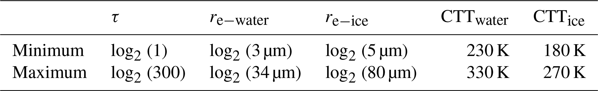
For the background covariance S_a, the variance of the state vector is used based on the minimum and maximum values (see Table 4). The uncertainties are assumed to be independent of each other, so the off-diagonal elements can be set to zero.

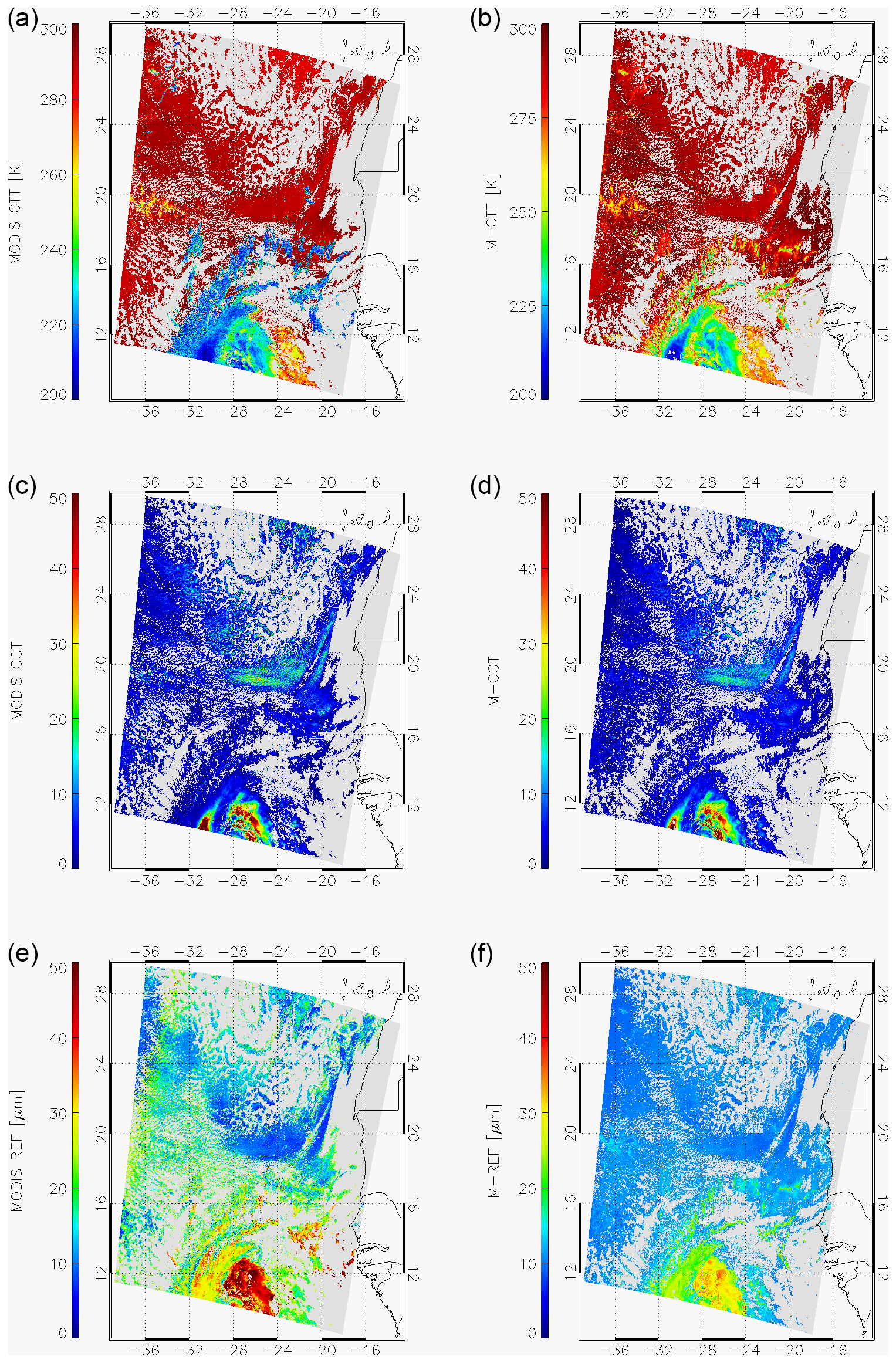
Figure 7 Case study from MODIS Terra granule at 12:20 UTC, 30 September 2021. Panels (a) and (b) show the cloud top temperature, (c) and (d) show the cloud optical thickness and (e) and (f) show the cloud effective radius at 1.6 µm. Panels (a), (c) and (e) correspond to the MOD06 L2 products, and (b), (d), and (f) correspond to the M-CLD.

2.5 Cloud optical and physical properties

The derived level 2 cloud properties from the OE retrieval schema are M-COT, M-REF and M-CTT. The M-CTT is further converted to M-CTH and M-CTP using the atmospheric profiles (X-MET) of pressure, temperature and height. These properties are accompanied by uncertainty measures derived from the OE algorithm. Figure 3 presents the full suite of M-COP products for one EarthCARE test scene, which refers to a realistic EarthCARE frame and MSI swath.

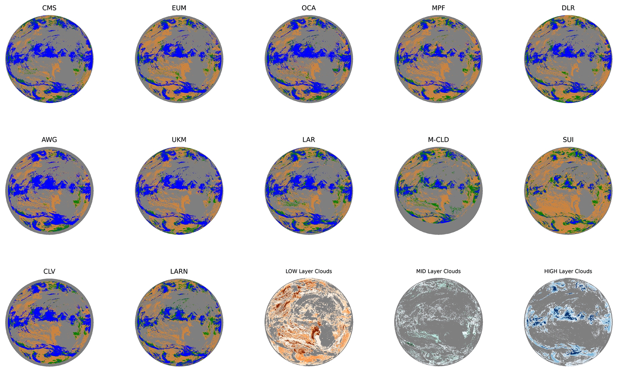
Figure 8 Cloud top pressure heights of the 13 algorithms submitted to ICWG, classified into three cloud classes – low (orange), middle (green) and high (blue) – based on the ISCCP classification for 13 June 2008 at 12:00 UTC. The combined cloud top pressure classes based on the consensus of all 13 ICWG algorithms are shown in the bottom row, separated into low (third MSG disc), middle (fourth MSG disc) and high (fifth MSG disc). Detailed information about the algorithms behind the acronyms in the titles are provided in Table 4 of Hamann et al. (2014).

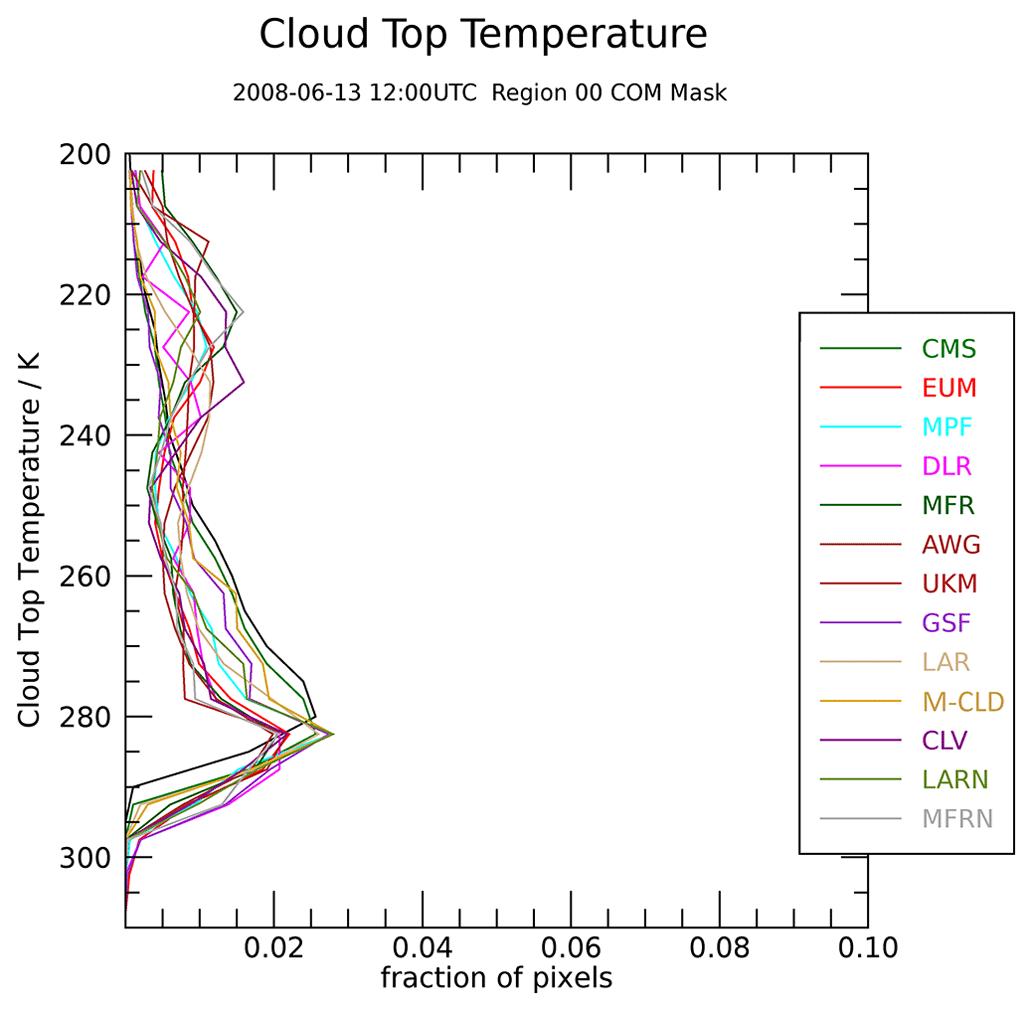
Figure 9 Histograms of the cloud top temperature of the 13 ICWG algorithms for 13 June 2008 at 12:00 UTC based on a common cloud mask. The M-CTT product is named here under the processor name M-CLD.

2.6 Cloud water path

The relation between the cloud optical thickness and the cloud effective radius is used to calculate the cloud water path based on the assumption of a homogeneous cloud. The cloud water path is calculated only indirectly due to the fact that the measurements from the MSI have no water absorption channel. The cloud water path CWP is defined as the integral of the liquid and/or ice water content throughout the profile of an ice or water cloud layer. MSI measurements of solar reflectance in shortwave atmospheric window channels are used to retrieve the cloud phase (water or ice on the top of the cloud; Hünerbein et al., 2023), cloud optical thickness (τ) and the effective radius (r_e). The cloud liquid/ice water path is calculated as a function of τ and r_e. The CWP is derived by using the following equation Stephens (1984):

$$\mathrm{CWP}={\displaystyle \frac{\mathrm{2}}{\mathrm{3}}}\mathit{\tau }{r}_{\mathrm{e}}{\mathit{\rho }}_{\mathrm{w},\mathrm{i}},$$

where ρ_w is the density of liquid water 1 g cm⁻³ and ρ_i is the density of ice 0.916 g cm⁻³. The CWP error is estimated from the combination of the error of τ and r_w,i as follows:

$$\mathrm{\Delta }\mathrm{CWP}=\mathit{\tau }\mathrm{\Delta }{r}_{\mathrm{e}}+r_{\mathrm{e}}\mathrm{\Delta }\mathit{\tau }.$$

3 Performance and intercomparison results

3.1 Evaluation with synthetic test scene

The M-COP algorithm performance has been tested by applying the M-CLD processor to different atmospheric test scenes created with the EarthCARE simulator. This is an end-to-end simulator for the EarthCARE mission capable to simulate the four instruments configurations for complex realistic scenes. Specific test scenes have been created from model output data (see Donovan et al., 2023). The 6000 km long frames include different types of clouds and aerosols as well as surface and illumination conditions. These synthetic scenes make it possible to evaluate and intercompare the different cloud properties, such as, for example, cloud liquid water path or the cloud effective radius, from active and passive sensors (Mason et al., 2023). The synthetic test scenes set up have been considered as the truth (named as such) to better understand and quantify the differences between the retrieved cloud properties based on the different measurement principles. It should be noted that the simulated test scenes are intended to quantify the performance of the different processors, but not to tune the retrievals because the test scenes strongly depend on the assumption made in the EarthCARE simulator. In the following, we present results obtained with the M-CLD processor for the HALIFAX scene (Donovan et al., 2023; van Zadelhoff et al., 2023). The scene starts with clouds over the Greenland ice sheet followed by high backscatter and extinction clouds down to 50^∘ N. A high ice cloud regime starting over eastern Canada down to 35^∘ N is followed by a low-level cumulus cloud regime embedded in a marine aerosol layer below an elevated dirty dust later around 5 km altitude. The results for the M-COP products for the HALIFAX scene are presented in Fig. 3 with the corresponding optimal estimation uncertainty. The M-COT uncertainty generally increases with increasing M-COT above 50, which is expected as the measurement at the non-absorption channel (VIS) gets saturated with increasing COT. The M-REF error shows clear separation between the detected cloud phase (Fig. 5), where ice clouds are associated with higher errors. Note that above 50^∘ N the solar zenith angle is higher than 84^∘ due to nighttime conditions. Therefore, M-COT/M-REF cannot be retrieved, and only the M-CTH is retrieved for this region. Furthermore, the simple M-CTH nighttime retrieval provides no uncertainty values.

In this evaluation, the 3D dataset input for the test scene (called the truth) is used to define the presence of clouds and to calculate the modelled cloud optical thickness. This is calculated from the extinction profiles of all hydrometeors multiplied by the layer thickness (Fig. 5) and compared with the retrieved M-COT. The true cloud optical thickness can also be retrieved in nighttime conditions. Furthermore, the truth includes values below 0.01, which are generally classified as clear sky by the M-CM cloud mask. This has been discussed in Hünerbein et al. (2023). Overall, the comparison with the true cloud optical thickness M-COT (Fig. 5) shows a good and promising agreement (Fig. 6).

3.2 MODIS data for testing M-COP

Additionally to the synthetic test scenes, the M-COP cloud algorithm has been tested against realistic satellite observation from MODIS. For that purpose, MODIS Terra L1b calibrated reflectance has been used as input for the M-CLD processor. The MODIS channels 1, 2, 6, 7, 29, 31 and 32 are closed to the seven MSI channels and taken to replace the MSI signal. The meteorological auxiliary data required as input for the M-CLD processor are replaced by the Copernicus Atmosphere Monitoring Service forecast data field. The cloud mask and phase (M-CM) are produced within the M-CLD processor and the results are described in the companion paper by Hünerbein et al. (2023). The three MODIS channels 1, 6 and 31 are used for the M-COP retrieval. The LUTs are not specifically adapted to the MODIS filter function, which will cause some uncertainties. Figure 7 shows a case study over the Capo Verde islands in the Atlantic Ocean. The right column shows the M-CTT, M-COT and M-REF (at 1.6 µm) results as retrieved by the M-CLD processor. The corresponding MODIS L2 products (MOD06_L2 collection 6.1; Platnick et al., 2015b, 2017) are given in the left column. The CTT comparisons show an underestimation of the cloud top height for high cirrus clouds, especially multilayer clouds, which will be further investigated if an improvement is possible by using multilayer flags. The COT comparison of M-CLD and MODIS exhibits an almost perfect match, with a correlation factor of 0.95 and a bias of less than 1. The REF comparisons show more differences, such as for ice clouds the M-REF have smaller particle sizes but for water clouds the sizes are slightly higher. It should be noted that different ice particle scattering models are used, which account for some of the variance. Compared with MODIS, the MSI cloud product shows, in general, a good agreement. The robustness of these results could be demonstrated by using longer time periods and also other regions, which is, however, not shown in this study.

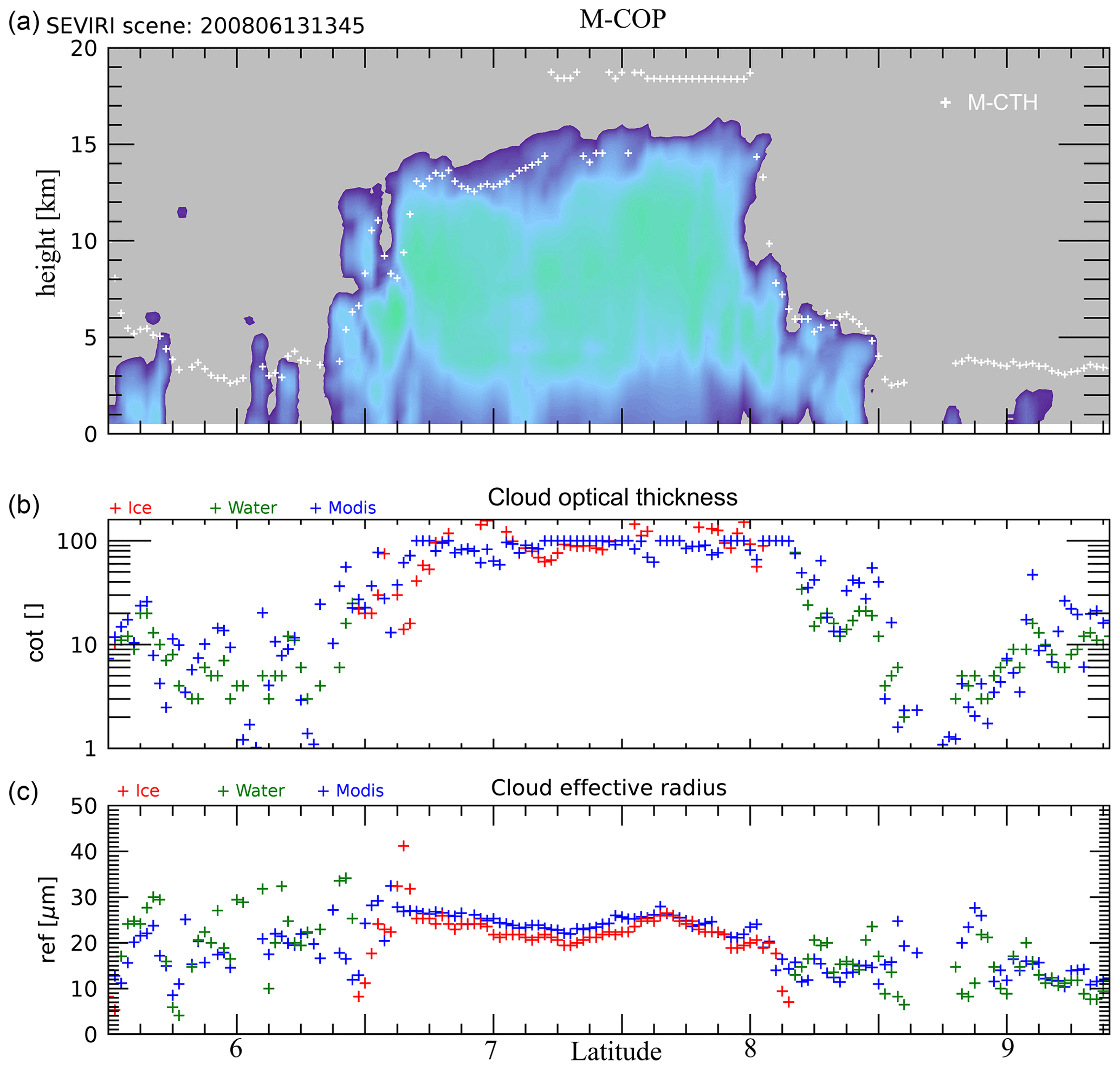
Figure 10 Selected CloudSAT, MODIS and M-COP (based on SEVIRI L1) cloud properties over West Africa with deep convection. Panel (a) shows cloud radar reflections with the M-CTH (white crosses). Panel (b) displays the MODIS-COT (blue) and the M-COT (with cloud phase; red: ice, green: water) on the track. Panel (c) presents the MODIS-REF compared with M-REF while M-REF is also separated between water and ice.

3.3 Intercomparison with other SEVIRI cloud products

The M-CLD cloud products have also been validated within the framework of the CGMS International Cloud Working Group (ICWG; Roebeling et al., 2013, 2015). The ICWG is a working group aimed at harmonizing and advancing quantitative cloud property retrievals. In support of its mission, the ICWG has assessed a large number of level 2 passive imager cloud parameter retrievals through intercomparison activities. The ICWG cloud assessments have focused on quantifying deterministic differences between level 2 cloud parameters (and their error estimates) and the statistical validation against superior reference datasets. This assessment so far has been limited to geostationary satellites, i.e. MSG with the SEVIRI instrument. SEVIRI provides similar channel settings to MSI except for the 2.2 µm channel, which is missing. The cloud parameters that have been part of the assessment are cloud mask, cloud top temperature, cloud top pressure, cloud top height, cloud phase, cloud optical thickness, effective particle size, cloud liquid water path, and cloud ice water path. As reference datasets, the main sources of information have been the cloud properties obtained from CLOUDSAT and/or CALIPSO observations and cloud liquid water path observations from passive microwave instruments (e.g. AMSR (advanced microwave scanning radiometer)). For a number of “golden days” different scientific institutions have contributed their cloud datasets for intercomparison, e.g. the EUMETSAT central facility, the Nowcasting SAF and the Climate Monitoring SAF, among others. The cloud properties retrieved from all MSG SEVIRI scans collected during 13 June 2008, 19 August 2015 and 21 July 2016 had to be submitted and served as the basis for the intercomparison (Hamann et al., 2014). It should be noted that the MSI M-CLD algorithm is developed for a polar-orbiting satellite and is adapted to the MSI specification, which leads to uncertainties in the adaptation to SEVIRI due to differences in central wavelength and spectral response function, radiative transfer simulations and generated look-up tables. The M-CLD processor has been directly applied to the SEVIRI observation.

Figure 8 shows the cloud top pressure obtained by 13 different retrievals for the noon scene of 13 June 2008 and the combined cloud top pressure separated into low, middle and high. The cloud top pressure is separated into three classes for the comparison: low (red), middle (green) and high (blue) based on the ISCCP classification. The zonal distribution of the cloud top pressure is comparable for all datasets. High clouds are present in the intertropical convergence zone. The combined cloud top pressure illustrates the disagreement for the anvil of the convective clouds within the intertropical convergence zone. Adjacent to them, low clouds are most common in the marine stratocumulus region between 30^∘ S and 30^∘ N and agree well between the algorithms. Note that the cloud masks differ between the algorithms, which also influences the mean cloud top pressure obtained by the algorithm. Some algorithms also limit the domain for retrieval due to large viewing or solar zenith angles and/or sun glint.

Figure 9 shows the histograms of the cloud top temperature from all the applied retrievals. A common cloud mask is used to calculate the individual CTT histograms. Different cloud occurrence frequencies are observed for the boundary layer clouds. Most histograms show a distribution with two cloud occurrence maxima, one around 230 K and a second one below 280 K. The weakness of M-CTT is the detection of multilayer clouds with high cirrus clouds in the upper troposphere. For example, the anvil of the deep convective storm systems classified as having medium instead of high cloud top height (see Fig. 8). This finding is also reflected in the histogram (Fig. 9, yellow curve) where the second maximum at 230 K is not present. It should be noted that the other algorithms take advantage of the SEVIRI CO₂ band, which MSI does not have.

Additionally, the A-Train constellation of earth-observing satellites (Stephens et al., 2002, 2018) of the comparison, the CloudSat (Marchand et al., 2008) and MODIS measurement (MYD06_L2; Platnick et al., 2015a), are re-gridded onto the SEVIRI grid. Five regions from the SEVIRI disc have been selected to study in more detail specific meteorological conditions. One example is a deep convection cell over West Africa presented in Fig. 10. On top, the CloudSat measurements on the A-Train track are compared with the M-CTH (Fig. 10, white crosses) and generally show a good agreement for most of the collocated observations. The M-CLD COT and REF values (red: ice phase; green: water phase) have been also compared to the L2 products from MODIS (Fig. 10, blue). The COT values between MODIS and MSI are in good agreement, while there is a slight overestimation of M-REF compared with MODIS for water clouds and underestimation for ice clouds. However, one should note that this is only a qualitative comparison for one case study, and a comprehensive assessment of the quality of the M-CLD products will be performed once real MSI observations are available.

4 Conclusions

This paper describes the baseline algorithms used to retrieve the optical and physical products (M-COP) from observations of the MSI instrument onboard the EarthCARE satellite. As such, M-COP is an essential part of the MSI cloud processor M-CLD. The cloud mask algorithm M-CM, which is an important input for M-COP, is described in the companion paper by Hünerbein et al. (2023). We described all significant components of the M-CLD processor to retrieve the M-COP products (Fig. A1). The algorithm is based on the widely used optimal estimation technique and simultaneously considers the shortwave and longwave MSI channels to obtain an optimal estimate of the targeted cloud properties, including an error estimate. The validation results demonstrate the comparability of M-COP results with those of similar operationally used algorithms. M-CLD is able to provide cloud optical and physical products in near real time on a global basis. It has to be realized, however, that the performance depends on the observation conditions including surface type (e.g. desert, sun-glint or ice), illumination and viewing geometry, and cloud type. The provision of uncertainty estimates as part of the M-COP products will enable an assessment of the situation-dependent retrieval uncertainty. The software will be embedded in the ESA processing framework.

The algorithm performance has been assessed using synthetic EarthCARE test scenes as well as satellite observations from the MODIS and SEVIRI instruments. Overall, the comparison with the test scene truth and the different imager cloud products shows encouraging results. The MODIS and SEVIRI imagers feature additional channels which provide further information, for example, for detecting thin clouds or identifying multilayer cloud situations (thin over thick). In particular, the cloud top height is observed to be biased low in multilayer situations, which are further investigated with the synergistic ATLID-MSI retrieval in Haarig et al. (2023).

The MSI solar channels show a spectral curvature non-linearity disturbance due to imperfect bandpass filters on the curved optical lenses (Wehr et al., 2023), which causes a spectral shift in across-track direction. This degradation of the spectral information content is currently under investigation, and it is planned to integrate mitigation measures in the M-CLD processor. Furthermore, the forward model RTTOV will be updated soon to its newest version 13.3, which includes the real MSI filter functions as one important update. During the commissioning phase, the configurable parameter of the processor will be still adjusted and optimized to improve the accuracy by using dedicated EarthCARE campaigns and geostationary satellite observations.

Appendix A

The MSI cloud processor consists of two main parts (see Fig. A1), which are sequentially processed. The M-COP relies on the availability of M-CM information as provided also by the M-CLD processor in the first step, which is described in Hünerbein et al. (2023).

Figure A1 Flowchart of the M-CLD processor.