the Creative Commons Attribution 4.0 License.
the Creative Commons Attribution 4.0 License.
 | 08 May 2024
Retrievals of aerosol optical depth over the western North Atlantic Ocean during ACTIVATE
Joseph S. Schlosser
David Painemal
Brian Cairns
Marta A. Fenn
Richard A. Ferrare
Johnathan W. Hair
Chris A. Hostetler
Longlei Li
Mary M. Kleb
Amy Jo Scarino
Taylor J. Shingler
Armin Sorooshian
Snorre A. Stamnes
Xubin Zeng
Aerosol optical depth was retrieved from two airborne remote sensing instruments, the Research Scanning Polarimeter (RSP) and Second Generation High Spectral Resolution Lidar (HSRL-2), during the National Aeronautics and Space Administration (NASA) Aerosol Cloud meTeorology Interactions oVer the western ATlantic Experiment (ACTIVATE). The field campaign offers a unique opportunity to evaluate an extensive 3-year dataset under a wide range of meteorological conditions from two instruments on the same platform. However, a long-standing issue in atmospheric field studies is that there is a lack of reference datasets for properly validating field measurements and estimating their uncertainties. Here we address this issue by using the triple collocation method, in which a third collocated satellite dataset from the Moderate Resolution Imaging Spectroradiometer (MODIS) is introduced for comparison. HSRL-2 is found to provide a more accurate retrieval than RSP over the study region. The error standard deviation of HSRL-2 with respect to the ground truth is 0.027. Moreover, this approach enables us to develop a simple, yet efficient, quality control criterion for RSP data. The physical reasons for the differences in two retrievals are determined to be cloud contamination, aerosols near the surface, multiple aerosol layers, absorbing aerosols, non-spherical aerosols, and simplified retrieval assumptions. These results demonstrate the pathway for optimal aerosol retrievals by combining information from both lidars and polarimeters for future airborne and satellite missions.
- Article
(5479 KB) - Full-text XML
-
Supplement
(384 KB) - BibTeX
- EndNote


Aerosol particles constitute an important component of the Earth's atmosphere by altering its radiative energy balance. Aerosols impact our climate system directly by scattering and absorbing solar and terrestrial radiation and indirectly by serving as cloud condensation nuclei (CCN) and ice nuclei (IN) (Lohmann and Feichter, 2005; Pöschl, 2005). Changing CCN and IN concentrations can influence the distribution of liquid water, ice, and mixed-phase clouds and the frequency of precipitation. The complex interaction of aerosols with clouds, radiation, and meteorology makes it difficult to probe the feedback and response of our climate system under a perturbation of anthropogenic or natural aerosols (Bellouin et al., 2020; Chen et al., 2014). In the most recent Sixth Assessment Report (AR6) of the Intergovernmental Panel on Climate Change (IPCC), aerosols still represent the largest uncertainty in the global radiative forcing (IPCC, 2023).
To disentangle aerosol–cloud interactions, it is imperative to collect adequate observations for robust statistics across a wide range of cloud regimes. The recent Aerosol Cloud meTeorology Interactions oVer the western ATlantic Experiment (ACTIVATE) epitomizes a coordinated effort to respond to this need (Sorooshian et al., 2023). Being one of the National Aeronautics and Space Administration (NASA) Earth Venture Suborbital-3 (EVS-3) missions, ACTIVATE has three objectives:
-
first, to quantify the underlying relationship between the aerosol number concentration, CCN concentration, and cloud drop number concentration;
-
second, to develop a better process-level representation of cloud properties and aerosol–cloud interactions in a hierarchy of numerical models;
-
finally, to evaluate state-of-the-art remote sensing instruments that are built for retrieving the aerosol and cloud properties (Sorooshian et al., 2019).
Aerosol optical depth (AOD) is a vertically integrated quantity of aerosol extinction coefficient, representing the column aerosol loading. It is one of the most widely used parameters to monitor the long-term evolution of aerosols at both global and regional scales (Andreae, 2009; Seinfeld et al., 2016). It is important to evaluate AOD retrievals and their associated uncertainties. An uncertainty of AOD retrievals of 0.01 could lead to an uncertainty of aerosol radiative forcing of ∼ 0.5 W m−2 (Chylek et al., 2003; Hansen et al., 1995; Mishchenko et al., 2004). Two approaches are regularly used to quantify uncertainties of AOD retrievals: propagated (prognostic) uncertainty and truth-based (diagnostic) uncertainty (Gao et al., 2022; Sayer et al., 2020). The former is a theoretical estimate which is obtained by considering measurement uncertainties, forward model uncertainties, and a priori assumptions via minimizing a suitable cost function. The latter is to compare the retrieval with a reference dataset. The two approaches are complementary to each other as the reference dataset can assess the theoretical estimate using appropriate statistical methods (Gao et al., 2022).
This work is focused on the second approach as two remote sensing instruments, the Research Scanning Polarimeter (RSP) and Second Generation High Spectral Resolution Lidar (HSRL-2), retrieved AOD over the western North Atlantic Ocean during ACTIVATE. Before proceeding, however, there is a catch, that is, the following question: how do we objectively assess these two datasets? Ideally, the error of a dataset should be quantified by comparing it with the “ground truth” (Caires and Sterl, 2003). Practically, the ground truth for AOD measurements is replaced by measurements from some ground-based instruments such as sun photometers in the AErosol RObotic NETwork (AERONET; Holben et al., 1998). But ground-based observations are unavailable over the study region, primarily an open ocean. Furthermore, all instruments and retrievals are subject to errors consisting of systematic bias and random noises (Stoffelen, 1998).
We propose to use a statistical method called triple collocation (TC) which partially circumvents the aforementioned issues. A third dataset is introduced, and the error characteristics of each dataset are determined with respect to the unknown ground truth. The most accurate dataset is then used to help design a simple, yet efficient, data flag to improve the quality of the other datasets. The physical processes that lead to the difference between RSP and HSRL-2 retrievals are discussed along with three case studies.
2.1 Overview of the ACTIVATE field campaign
The ACTIVATE field campaign started in February 2020 and concluded in June 2022 with six deployments. There were winter and summer deployments each year, roughly covering November to March and May to September, respectively (Sorooshian et al., 2023). While it is recommended to explicitly label the year and season of each deployment, for simplicity we refer to the three winter and three summer deployments collectively as the “winter” and “summer” deployments.
Two aircraft, the King Air (high-flying) and Falcon (low-flying) from the NASA Langley Research Center (LaRC), were used to carry out spatially coordinated flights over the western North Atlantic Ocean. The total number of flights for the King Air and Falcon are 174 and 168, respectively, with 162 being joint flights. The remote sensing instruments in this study were flown on the King Air which logged a total of 592 flight hours (Sorooshian et al., 2023).
Most of the 3–4 h flights were based at NASA LaRC, with a notable exception being 17 flights based in Bermuda during June 2022 (Fig. 1). Due to air traffic considerations associated with military restricted areas, the aircraft usually had to transit through one of three waypoints, OXANA, ZIBUT, and ZIZZI.
Figure 1The ACTIVATE study region and NASA Langley King Air flight tracks between 2020 and 2022. Summer and winter deployments are indicated in red and blue, respectively. The two campaign bases, NASA Langley Research Center (LaRC) and Bermuda, and three commonly used waypoints, OXANA, ZIBUT, and ZIZZI, are annotated with arrows.
2.2 Research Scanning Polarimeter
The Research Scanning Polarimeter (RSP) is a remote sensing instrument that uses three pairs of optical assemblies to simultaneously measure linear polarization of the intensity at four polarization azimuths and nine spectral channels centered at 410, 470, 555, 670, 865, 960, 1590, 1880, and 2264 nm for each scene (Cairns et al., 1999, 2003). The first three components of the Stokes vector (I, Q, and U) are then derived from the measurement. RSP operates by continuously scanning the field of view (14 mrad) over ± 55° from viewing zenith (∼ 140 views) along the flight track, which samples at 0.8° interval (Alexandrov et al., 2012; Cairns et al., 2003). Each RSP scan consists of measurements from all different viewing angles. That is, each target at the cloud top or ground surface is swept from different scans at different viewing angles. These actual scans are assembled into virtual scans for each target at nadir (Alexandrov et al., 2012).
The aerosol properties are retrieved using the RSP Microphysical Aerosol Properties from Polarimetry (MAPP) algorithm version 1.48, consisting of a vector radiative transfer model and a Mie code (Stamnes et al., 2018; Schlosser et al., 2022). The retrieval algorithm is geared for field campaigns which desire both speed and flexibility. Speed is important for field campaigns because data are needed as soon as possible for preliminary data analysis and flight planning. To speed up computations, the Mie code assumes particles are spherical and homogeneous. Flexibility is also important because the traditional pre-computed Mie lookup table approach requires constant aircraft altitudes and aerosol locations, which limits the choice of flight patterns. To remain flexible, both the vector radiative transfer and Mie computations are done on the fly.
The retrieval algorithm uses an optimal-estimation method (Rodgers, 2000) to minimize a cost function χ2 that describes the difference between the observations and a forward model for aerosol parameter retrievals and includes a term that takes into account of a priori knowledge of aerosol properties. The cost function χ2 is formulated and described in detail by Stamnes et al. (2018) and includes a metric describing the goodness of fit between the forward model and RSP measurements, called the normalized cost function χ’. Here we only consider retrievals successful when χ’ is less than 0.15. As regards the a priori best guess, we adopt an elementary and conservative approach by taking the mean of the permissible range of each aerosol parameter, which is also utilized as the first guess.
The current version of algorithm assumes that the aerosol size distribution is bimodal: one fine mode and one coarse mode (Stamnes et al., 2018). Aerosol properties such as AOD, refractive index, and effective radius are retrieved separately for the two modes. The coarse mode is assumed to be composed of non-absorbing sea salt particles with a refractive index equivalent to that of water. The coarse-mode aerosol top height is assumed to be 1 km, while the fine-mode aerosol top height is retrieved (Schlosser et al., 2022).
The theoretical ±1σ accuracy of the MAPP algorithm for AOD is ± 0.02 (Stamnes et al., 2018). The practical accuracy of RSP has been estimated in several field campaigns through comparison with sun photometers, but most of them took place over land. Knobelspiesse et al. (2011) found that the mean error of RSP relative to the Ames Airborne Tracking Sunphotometer (AATS-14) is 0.057 at 532 nm for a forest fire event during the Arctic Research of the Composition of the Troposphere from Aircraft and Satellites (ARCTAS) field campaign. Di Noia et al. (2017) compared RSP aerosol retrievals against AERONET during the POlarimeter DEfinition EXperiment (PODEX) and Studies of Emissions and Atmospheric Composition, Clouds and Climate Coupling by Regional Surveys (SEAC4RS) field campaigns in 2012 and 2013, respectively. The bias and root mean squared error of these retrievals at 500 nm are 0.02 and 0.04, respectively. Fu et al. (2020) compared measurements from four multi-angle polarimeters, including RSP, against AERONET during the Aerosol Characterization from Polarimeter and Lidar (ACEPOL) field campaign over the western part of the United States in 2017. The standard deviations between RSP and AERONET are 0.035, 0.027, and 0.014 at 380, 440, and 675 nm, respectively.
In this study, we use the RSP level 2 aerosol product which includes column-averaged aerosol optical and microphysical parameters and ocean color parameters. The RSP data are averaged horizontally over 10 scans from the level 1C product, with a temporal resolution of ∼ 9.3 s and an along-track spatial resolution of ∼ 1 km.
2.3 Second Generation High Spectral Resolution Lidar
The Second Generation High Spectral Resolution Lidar (HSRL-2) is an airborne multi-wavelength instrument which uses the HSRL technique to separate the aerosol and molecular backscatter signals at 355 and 532 nm and the standard backscatter lidar technique at 1064 nm. HSRL-2 can vertically resolve the backscatter coefficient β and depolarization δ at 355, 532, and 1064 nm and extinction coefficient α at 355 and 532 nm (Burton et al., 2018; Hair et al., 2008; Ferrare et al., 2023). Because of the incorporation of three backscatter and two extinction measurements, the instrument is also referred to as a “3β+2α” lidar (Burton et al., 2016). The field of view of HSRL-2 is 1 mrad (Schlosser et al., 2022). AOD is derived from the aerosol backscattering coefficient using the difference in molecular return signals (Hair et al., 2008).
The performance of HSRL-2 measurements has been compared with various instruments. For example, Shinozuka et al. (2013) showed that the root mean squared difference of 532 nm AOD between the Spectrometer for Sky-Scanning, Sun-Tracking Atmospheric Research (4STAR) and HSRL-2 is 0.01 during the 2012 Two-Column Aerosol Project (TCAP) campaign. Sawamura et al. (2017) showed outstanding agreement between the AERONET and HSRL-2 from over 300 profiles collected during the 2013 Deriving Information on Surface Conditions from COlumn and VERtically Resolved Observations Relevant to Air Quality (DISCOVER-AQ) campaign. Stamnes et al. (2018) found that the root mean squared deviations between RSP and HSRL-2 AOD at 532 nm are ∼ 0.07 during TCAP and ∼ 0.04 during the 2014 Ship-Aircraft Bio-Optical Research (SABOR) campaign.
In this study, we use the 10 s aerosol profile product of which spatial resolution is ∼ 1 km. We also use the following derived products: mixing layer height (MLH) and aerosol identifier. MLH is estimated from the sharp gradients of HSRL-2 aerosol backscatter profiles at 532 nm (Scarino et al., 2014). A Haar wavelet transform is first applied to the vertical profiles to identify the transition zone above the top of the aerosol mixed layer, and then MLH is defined as the altitude of the maximum value after the wavelet transform. The information of aerosol identifiers (or types) is based on the HSRL aerosol classification scheme (Burton et al., 2012) which identifies aerosols using the lidar ratio, depolarization, backscatter color ratio, and spectral depolarization ratio from HSRL-2 measurements. Eight types of aerosols are classified, including dust, polluted marine, fresh smoke, smoke, urban, marine, a dusty mix, and ice. The algorithm has been shown to improve a similar scheme for the Cloud-Aerosol Lidar with Orthogonal Polarization (CALIOP) instrument (Burton et al., 2013; Ferrare et al., 2023).
To expedite comparison with gridded global reanalysis data, selected instantaneous meteorological fields from the Modern-Era Retrospective Analysis for Research and Applications, version 2 (MERRA-2; Gelaro et al., 2017), are interpolated to the HSRL-2 curtains along the flight tracks. These 3-hourly MERRA-2 variables have a horizontal resolution of 0.5° × 0.625° (latitude × longitude) on 42 pressure levels from 1000 to 0.1 hPa.

Figure 2Distribution of RSP (blue) and HSRL-2 (red) AOD for the whole field campaign period (2020–2022). Each bin is 0.025. Mean values (dashed colored lines) and selected statistics (mean, median, SD, and IQR) are also shown.
2.4 Other ACTIVATE datasets
The King Air navigational data for RSP and HSRL-2 are provided by an Applanix 610 system at 2 Hz, including flight date, time, longitude, latitude, altitude, and other aircraft motion variables (Sorooshian et al., 2023). Two cameras were mounted on the King Air: one facing nadir and the other facing forward (Sorooshian et al., 2023). The images collected from the airborne cameras are used to identify the presence of clouds above and below the aircraft. Recently, a cloud detection neural network (CDNN) algorithm was developed to speed up the cloud identification process by training and testing the camera imageries via convolutional neural network, which resulted in above-aircraft and below-cloud cloud mask products at 1 Hz (Nied et al., 2023). The accuracy of the forward-facing CDNN is 96 %, calculated through validation against human-labeled testing data. The Falcon relative humidity data are provided by a diode laser hygrometer (DLH) with an uncertainty of 0.1 ppmv (Diskin et al., 2002).
Table 1Monthly RSP and HSRL-2 AOD statistics. SD and IQR denote standard deviation and interquartile range, respectively.

2.5 Moderate Resolution Imaging Spectroradiometer
The Moderate Resolution Imaging Spectroradiometer (MODIS) is an imaging instrument with 36 spectral channels ranging from 0.41 to 14.5 µm. The instrument collects data at three nadir spatial resolutions (250 m, 500 m, and 1 km) (Remer et al., 2005). As part of the NASA Earth Observing System, two almost identical MODIS sensors were launched on the Terra and Aqua satellites in December 1999 and May 2002, respectively. Both satellites observe the Earth from a polar-orbiting, sun-synchronous orbit at an altitude of ∼ 700 km. The equatorial overpass times for the descending mode of Terra and the ascending mode of Aqua are 10:30 and 13:30 local solar time, respectively. The swath of each scan is 2330 km × 10 km (across track × along track at nadir) (Levy et al., 2013). Seven bands are used for aerosol retrievals.
In this study, we use the following level 2 aerosol products from the MODIS Collection 6.1: MOD04_3K from Terra and MYD04_3K from Aqua. The horizontal resolution is 3 km × 3 km at nadir. The Dark Target (DT) algorithm is used to retrieve the 3 km aerosol product (Levy et al., 2013; Remer et al., 2013). The algorithm is complicated (see, for example, Remer et al., 2005). Generally, each grid box consists of pixels (i.e., each pixel is at 500 m resolution at nadir). The algorithm checks the number of good pixels in each grid box using multiple criteria before doing the actual inversion. Therefore, the existence of cloudy pixels does not stop the retrieval as long as there are enough good pixels within the same grid box (Remer et al., 2013). Note also that the cloud pixels would not be included during the inversion.
To compare with the RSP and HSRL-2 AOD at 532 nm, the MODIS AOD at 550 nm is converted to 532 nm using the Ångström exponent from the MODIS AOD at 470 and 550 nm. Compared to AERONET, the expected error for the DT algorithm is ) (Remer et al., 2013).
2.6 Cloud-Aerosol Lidar with Orthogonal Polarization
The Cloud-Aerosol Lidar with Orthogonal Polarization (CALIOP) is the primary instrument that was launched on the Cloud-Aerosol Lidar and Infrared Pathfinder Satellite Observations (CALIPSO) satellite in April 2006 (Winker et al., 2009). We use the CALIOP level 3 stratospheric aerosol profile products which are based on version 4 of CALIOP level 1B and level 2 datasets (Kar et al., 2019). The horizontal resolution of the monthly stratospheric AOD data is 5° × 20° (latitude × longitude). To maximize the length of available data, we stitch the datasets from versions 1.00 and 1.01. The version 1.01 begins in July 2020.
3.1 Traditional metrics
To summarize the distribution of an AOD dataset, it is common to use mean and standard deviation (SD) to measure its central tendency and dispersion, which are known to be affected by outliers. The median and interquartile range (IQR= the third quartile minus the first quartile) are also used as they are more robust against outliers.
To evaluate AOD between two collocated datasets X and Y, each having n elements, we use the following metrics:
where r, MB, and RMSD are Pearson's correlation coefficient, the mean bias, and the root mean squared deviation, respectively, and the overbar denotes the mean value of a dataset.

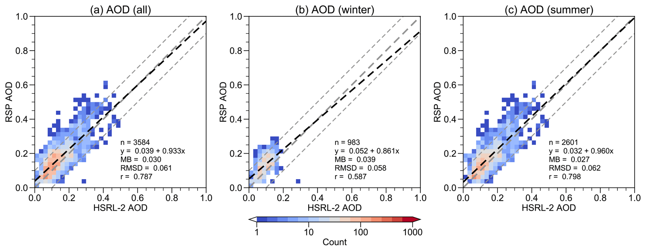
Figure 3Two-dimensional histograms of RSP and HSRL-2 AOD. (a) All data. (b) Winter deployments only. (c) Summer deployments only. Bin size is 0.025 for both instruments. In each plot, the linear fit (dashed black), 1 : 1 line (thick dashed gray), ±0.1 intervals (thin dashed gray), and selected error metrics are shown.
3.2 Triple collocation
Triple collocation (TC) is a statistical method that estimates error statistics of a target variable from three independent and collocated datasets (Stoffelen, 1998). The method does not require any one of the triplet items to be the ground truth. It has been used for characterizing errors in a wide range of geophysical variables such as sea surface temperature (O'Carroll et al., 2008), soil moisture (Draper et al., 2013), and ocean wave height (Caires and Sterl, 2003; Janssen et al., 2007).
In this study, we take advantage of three available AOD retrievals from RSP, HSRL-2, and MODIS. To start with, each dataset is considered as an estimate of the (unknown) ground truth. Therefore, a functional relationship (or an error model) is assumed to exist between each dataset and the ground truth to account for the potential deviation from the truth. The linear relationship is one of the simplest error models. Some linear error models are discussed in detail in Zwieback et al. (2012). We adopt an affine (also linear) model for the AOD datasets:
where τi () represents the AOD from dataset i; Θ is the true AOD; and ai, bi, and ϵi are the additive bias, multiplicative bias, and random error from dataset i, respectively. To simplify the notation, we assign RSP=1, HSRL-2=2, and MODIS=3.
Together with the error model being linear, the following assumptions are made (Gruber et al., 2016). First, the random error has zero mean (E[ϵi]=0). Second, the random error is uncorrelated with the true AOD . Third, the random error of different products is uncorrelated with each other . Lastly, the additive and multiplicative biases are time invariant.
The equations of variance and covariance between the collocated datasets can then be obtained (McColl et al., 2014; Stoffelen, 1998) by
where is the truth variance and is the error variance. Note that .
The error variances are then solved with the help of the above assumptions (McColl et al., 2014):
McColl et al. (2014) extended the theory by solving the correlation coefficient of each dataset with respect to the ground truth, resulting in
where sgn is the signum function; there is a sign ambiguity for each ri, but practically all the AOD datasets are expected to be positively correlated with the unknown true value. If the ground truth is known, the correlation coefficient can be easily computed from Eq. (1). However, if the ground truth is unknown, the TC method enables the computation of the correlation coefficient from Eqs. (10)–(12).
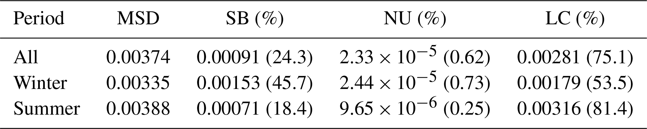
Table 2Mean squared deviation (MSD) decomposition of RSP and HSRL-2 AOD.
Table 3Triple collocation analysis of RSP, HSRL-2, and MODIS AOD.
3.3 Data alignment
To ensure the robustness of triple collocation analysis, we attempt to minimize the representation error due to the different support scales between the AOD datasets. The 10 s HSRL-2 data are coarsened to 30 s resolution by horizontally averaging three consecutive data points, which results in a 3 km product. Then, all RSP data points within the same 30 s window are averaged. To minimize cloud impact, all HSRL-2 and RSP data points must be valid within the same window. The data alignment and aggregation result in 6988 pairs of data from 134 flights.
4.1 Comparison of RSP and HSRL-2
The design of ACTIVATE to take place over the northwest Atlantic across different seasons was partly to characterize aerosol–cloud interactions across a wide range of aerosol conditions (Sorooshian et al., 2019). The overall distribution of RSP and HSRL-2 AOD is shown in Fig. 2, which demonstrates that a broad range of values was observed. The mean values of RSP and HSRL-2 AOD from 6988 pairs for the whole field campaign period are 0.173 and 0.120, respectively. RSP has a higher standard deviation than HSRL-2 (0.109 vs. 0.074). Both the mean and standard deviation are sensitive to outliers, so the median and interquartile range are also computed. The mean and median differences between RSP and HSRL-2 are about the same (0.053 vs. 0.047) and the interquartile range of RSP is larger than HSRL-2.
Table 1 shows the monthly breakdown of the AOD statistics. More than 80 % of data points come from March, May, and June. The largest mean AOD happens in May, August, and September for both instruments, and the median AOD corroborates the corresponding maxima. The same months also exhibit the largest variations as confirmed from the values of both standard deviation and interquartile range. The mean AOD is smallest in January and November, although the number of samples in winter is somewhat inadequate. The seasonal difference is largely consistent with Corral et al. (2021), who used coastal monitoring sites and a reanalysis product to study the regional AOD properties. During summer, there are more African dust events (Aldhaif et al., 2020) and more biomass burning events originating from North America (Mardi et al., 2021).
Figure 4Two-dimensional histograms of the triple-collocated AOD datasets. Bin sizes are 0.02 for both instruments. (a) RSP vs HSRL-2. (b) MODIS vs HSRL-2. (c) MODIS vs RSP. In each plot, the linear fit (dashed black), 1:1 line (thick dashed gray), ±0.1 intervals (thin dashed gray), and selected performance metrics are shown.
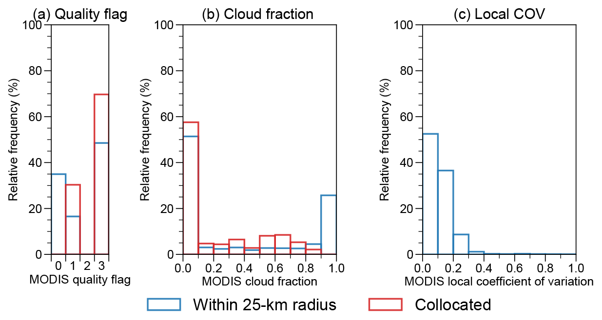
Figure 5Histograms of the MODIS AOD dataset. (a) Quality flag. (b) Cloud fraction. (c) Local coefficient of variation. Red color represents all the triple-collocated MODIS data points. Blue color represents all MODIS data points within a 25 km radius of RSP/HSRL-2.
The discrepancy between RSP and HSRL-2 AOD is shown in Fig. 3. Around 80 % of data points are within ± 0.1 intervals (Fig. 3a). The correlation coefficient r, RMSD, and MB are 0.727, 0.092, and 0.053, respectively. Most of the extreme outliers occur during the summer deployments (Fig. 3b–c).
A complementary approach of analyzing the deviation between RSP and HSRL-2 is to examine their mean squared deviation (MSD=RMSD2) decomposition. If two datasets x and y are identical to each other, all data points fall onto the 1 : 1 line (y=x, thick dashed gray lines in Fig. 3), and MSD equals zero. If there are discrepancies between two datasets (i.e., MSD>0), a linear fit (dashed black lines in Fig. 3), where a is intercept and b is slope, quantifies the deviations from 1 : 1 line with a≠0 and/or b≠1. Here we use the MSD decomposition proposed by Gauch et al. (2003),
where SB is squared bias, NU is non-unity slope, LC is lack of correlation, overlines denote the mean values, σ is standard deviation, r is the correlation coefficient between x and y, and b is the slope of the regression line of y on x.
Such partitioning has a straightforward geometric meaning for all three components. SB represents the translation of the linear fit from 1 : 1 line when there is a systematic bias, NU represents the rotation of linear fit when the slope b becomes different from 1, and LC represents the scattering of data points. The MSD decomposition in Table 2 shows that data scattering is the main contribution to the MSD for both winter and summer deployments. Systematic data bias is more severe in winter than in summer although the magnitude of bias is smaller in winter.
A question naturally arises from the above analysis as to which dataset is more accurate. Traditional metrics cannot answer this question because there is no available reference dataset over the western North Atlantic Ocean. To overcome this issue, we are motivated to carry out the triple collocation analysis.
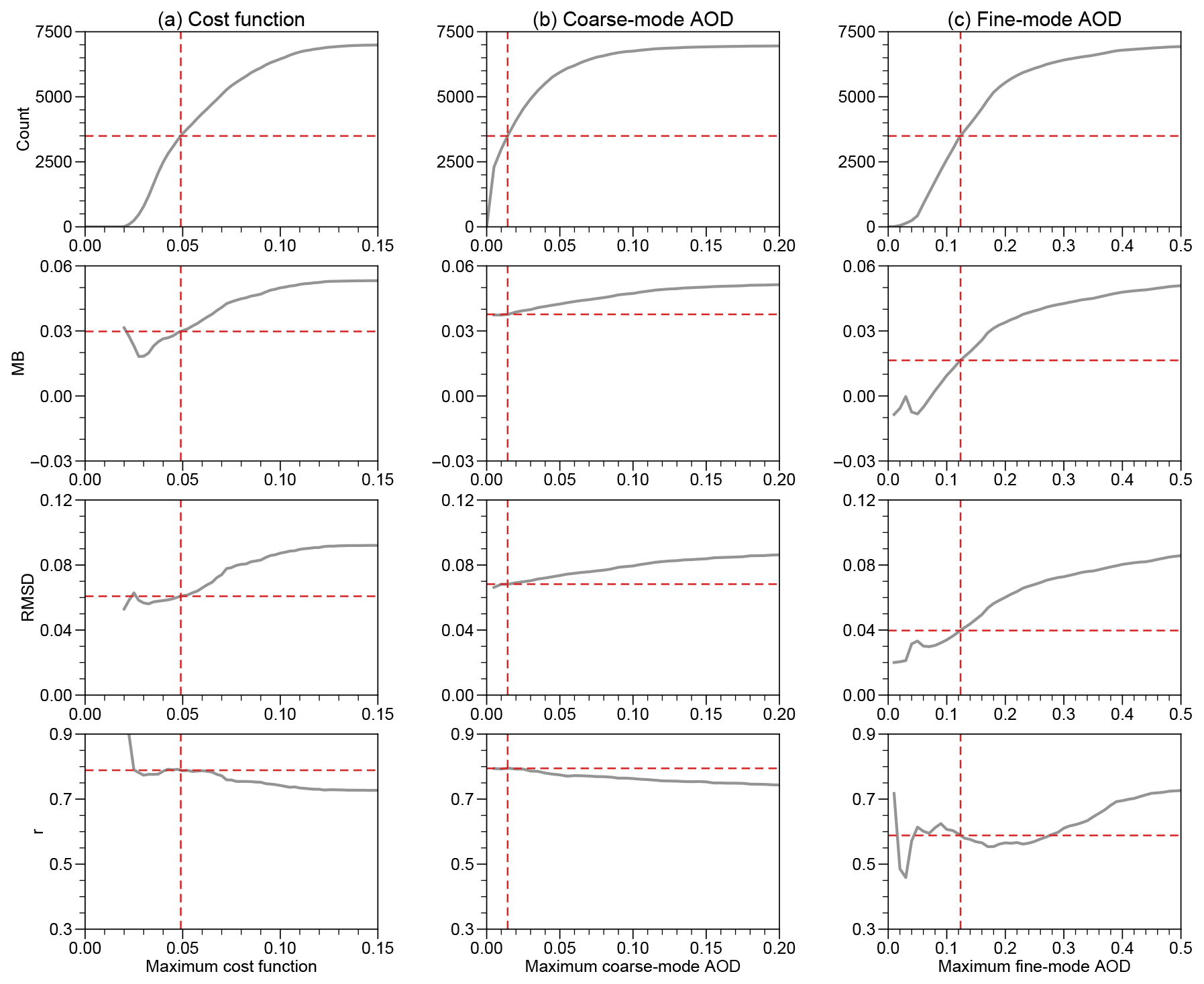
Figure 6Sensitivity of the performance of RSP filter criterion candidates. (a) Maximum normalized cost function (left column). (b) Maximum coarse-mode AOD (middle column). (c) Maximum fine-mode AOD (right column). In each plot, we calculate a performance metric as a function of criterion candidate threshold. As a result, the number of data points decreases when the criterion gets more stringent (smaller value). Intersecting dashed red lines indicate 50 % of the data points (y axis) meet the criterion threshold (x axis). First to fourth rows show, in order, the number of valid data points, mean bias, root mean squared deviation, and correlation coefficient.
4.2 Triple collocation analysis
We introduce MODIS AOD as the third dataset. For each pair of RSP and HSRL-2 data, we collocate the closest MODIS data point within ± 60 min and 25 km, which is deemed suitable for mesoscale aerosol variabilities (Anderson et al., 2003). The collocation process results in 2344 triplets, roughly 34 % of the original data points. Zwieback et al. (2012) suggested that at least 500 triplets are needed for robust error estimates.
Table 3 summarizes the error metrics of the three instruments. HSRL-2 has the lowest error standard deviation () and highest correlation coefficient (rHSRL-2=0.926) with respect to the true underlying values. After triple collocation, data scattering not only prevails between RSP and HSRL-2 (Fig. 4a) but also occurs between RSP and MODIS (Fig. 4c). HSRL-2 also maintains relatively higher correlation coefficients with both RSP and MODIS (Fig. 4a–b). The results suggest that HSRL-2 is the most accurate dataset among the three. Note that MODIS AOD corresponds to the whole atmospheric column, whereas RSP and HSRL-2 AOD correspond to the column below the aircraft. Therefore, MODIS AOD should be slightly larger than RSP and HSRL-2 AOD due to the contribution above the aircraft. The mean bias shows that MODIS is larger than HSRL-2 (Fig. 4b), but RSP is larger than MODIS (Fig. 4c). This suggests that it is more likely that RSP has a high bias over HSRL-2, not that HSRL-2 has a low bias over RSP (Fig. 3).
The result of the triple collocation analysis can be affected by a multitude of factors. Several factors related to MODIS data quality are discussed as follows.
First, MODIS provides a data quality flag which ranges from 0 to 3, with 3 being the best quality. Levy et al. (2013) recommend using data with non-zero quality flags. Figure 5a shows that all triple-collocated data points are at least 1 (red), which is much higher than all MODIS data points within a 25 km radius of RSP/HSRL-2 data points (blue). A related quantity is MODIS cloud fraction, which indicates possible cloud contamination. Figure 5b shows that the cloud fraction of over 55 % of triple-collocated data points is less than 0.1. The influence of excluding inferior MODIS collocated points is summarized in Table 3. While the error metrics of MODIS improve, there is little change for RSP and HSRL-2 which does not justify giving up 30 %–40 % of collocated data.
Second, since the Terra and Aqua satellites together provide only two overpasses during daytime because of their sun-synchronous orbits, we combine both datasets to maximize the number of files for collocation. This combination approach was adopted and tested in Antuña Marrero et al. (2018) by comparing 7-year Aqua, Terra, and Aqua + Terra data separately with measurements from an AERONET site. Generally, RMSD, MB, and r do not differ much in all cases (Table 5 in Antuña Marrero et al., 2018), which gives us confidence to combine Terra and Aqua data. We also performed sensitivity tests on the data quality of the third dataset and on the potential bias between two satellites using a synthetic data approach, which is included in the Supplement Sect. S1. The major conclusion is that the robustness of the error metrics is more sensitive to the number of data points rather than the data quality.
Third, collocation with the nearest MODIS data point may introduce bias when there is a spatial gradient of aerosols. Although it is generally difficult to evaluate the influence of the spatial gradient of aerosols, we adapt the local coefficient of variation (LCOV) from Anderson et al. (2003), which is the ratio of standard deviation and mean of all MODIS data points within a certain radius R of collocated RSP/HSRL-2 data points. In this case, R=25 km. Figure 5c shows that around 50 % and 90 % of LCOV are less than 0.1 and 0.2, respectively. An LCOV of 0.1 means that for a normally distributed random variable, 68 % of data points are within 10 % of the mean (Anderson et al., 2003). Similarly, 68 % of data points are within 20 % of the mean when the LCOV is 0.2. The mean HSRL-2 AOD is ∼ 0.1; therefore, most of the local AOD variation is estimated to be within 0.02, which is smaller than the expected error of the Dark Target algorithm. Interestingly, the current result is similar to the LCOV distributions obtained in Anderson et al. (2003) at similar spatial scale. Table 3 shows that including MODIS data points at high LCOV environs does not affect the assessment on the error metrics of RSP and HSRL-2.
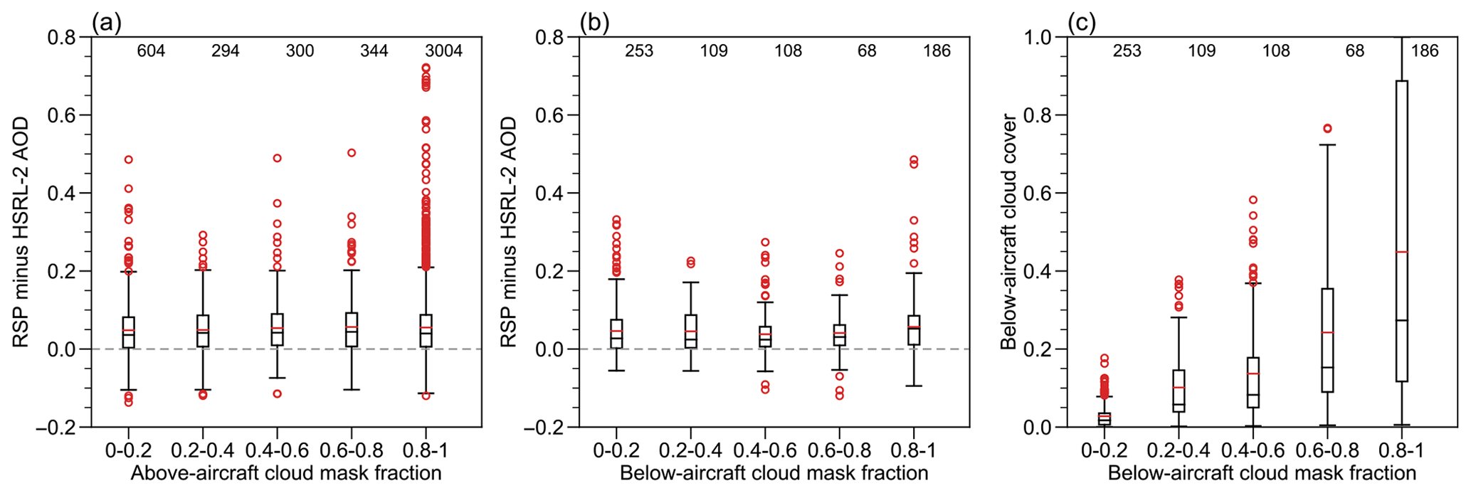
Figure 8Cloud impact on the bias between RSP and HSRL-2. (a) Bias-grouped by above-aircraft cloud mask fraction. (b) Bias-grouped by below-aircraft cloud mask fraction. (c) Cloud cover grouped by below-aircraft cloud mask fraction. Numbers at the top indicate the number of each data group. The box and whiskers indicates the variability of each group (box, first and third quartiles; black line in box, median; red line in box, mean; whiskers, a distance of 1.5 × IQR beyond the first and third quartiles; red circles, outliers).
4.3 RSP filter
The triple collocation analysis indicates that the most accurate AOD dataset over the western North Atlantic Ocean is HSRL-2 and paves the way for improving the data quality of RSP: the aim is to design a simple RSP filter to reduce disagreement between the two instruments. Three guiding principles are set. First, the filter should effectively get rid of outliers as suggested from the result of MSD decomposition (Table 2). Second, at the same time, the filter should keep as many data points as possible. Third, the criterion should be independent of HSRL-2 properties.
Three filter candidates are sought, including RSP normalized cost function χ′, coarse-mode AOD τc, and fine-mode AOD τf. The normalized cost function χ′ quantifies the performance of the vector radiative transfer model in the RSP-MAPP algorithm (Stamnes et al., 2018). Although it is tempting to use the total RSP AOD to filter out outliers, it is anticipated to be only effective for summer data because on average AOD is higher and fluctuates more during summer deployments (Table 1). Instead, τc and τf are chosen as they are part of retrieved parameters. For a successful retrieval, other than χ′ being lower than 0.15, the algorithm also requires that and . Because τc and τf are rarely larger than 0.2 and 0.5, respectively, lowering either may help eliminate outliers.
The filter candidates are tested by iteratively decreasing the maximum value allowed in the dataset, and three performance metrics (r, MB, and RMSD) are evaluated (Fig. 6). For a balanced candidate, it is expected that when the criterion gets more stringent, r should increase, and MB and RMSD should decrease at the same time. It is clear that the fine-mode AOD does not qualify because r generally decreases, while the maximum allowed fine-mode AOD is reduced (Fig. 6c). In other words, constraining the fine-mode AOD will lead to more data outliers, which goes against one of our principles. The remaining cost function and coarse-mode AOD are balanced candidates. A relatively fair way to compare the two balanced candidates is to focus on their performance metrics when 50 % of data points are left (intersection of dashed red lines in Fig. 6a–b). That means the ranges of cost function and coarse-mode AOD are 0 to 0.049 and 0 to 0.014, respectively. Compared to the coarse-mode AOD, the cost function performs better on the whole. Therefore, the cost function is regarded as the best simple filtering criterion. It has two additional benefits. First, it is globally applicable. Second, it also allows offline post-processing. For simplicity, the cost function threshold is set to be 0.05 thereupon.
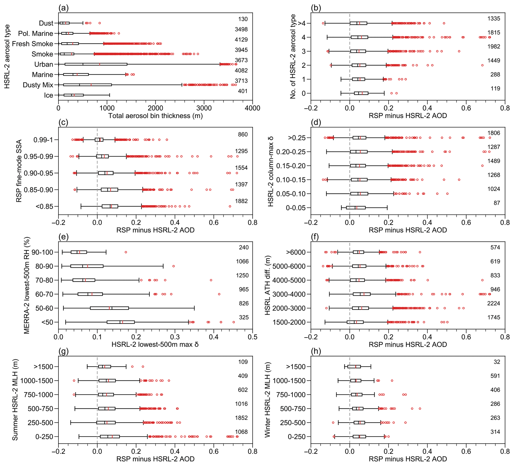
Figure 9Same as Figure 8 but for aerosol impact. (a) Average HSRL-2 aerosol column total thickness grouped by HSRL-2 aerosol type. (b) Bias-grouped by the number of HSRL-2 aerosol types. (c) Bias-grouped by RSP fine-mode single-scattering albedo (SSA) at 532 nm. (d) Bias-grouped by the HSRL-2 column-maximum 532 nm depolarization ratio δ532. (e) The maximum HSRL-2 δ532 at the lowest 500 m grouped by the collocated MERRA-2 relative humidity (RH). (f) Bias-grouped by the difference of aircraft altitude and HSRL-2 (effective) aerosol top height (ATH). (g) Bias-grouped by HSRL-2 mixed layer height (MLH) during summer deployments. (h) Bias-grouped by HSRL-2 MLH during winter deployments. Numbers on the right indicate the number of each data group.
To evaluate the cost function filter, we perform the comparison between RSP and HSRL-2 again (Fig. 7). All metrics generally improve. Compared to 80 % in Fig. 3a, more than 89.8 % of data points are now within ± 0.1 intervals after filtering. By analyzing MSD decomposition before and after filtering (Tables 2 and 4), it is found that the filter is effective in reducing MSD during summer deployments by cutting down around 80 % of the systematic bias.
4.4 Why do RSP and HSRL-2 disagree with each other?
Stamnes et al. (2018) suggested some possible sources of the discrepancies between two instruments: (i) aerosols above the aircraft, (ii) clouds above the aircraft, (iii) aerosols near the aircraft, (iv) three-dimensional effects due to clouds surrounding the aircraft, (v) aerosols close to the surface (within 100 m), (vi) multiple aerosol layers from different types of aerosol, (vii) presence of absorbing aerosols, (viii) presence of non-spherical aerosols, and (ix) intrinsic retrieval and measurement uncertainties. These factors are examined using the available field campaign data.
To streamline the analysis, the aforementioned factors can be broadly organized into two groups: cloud and aerosol impacts. We use the above-aircraft and below-aircraft cloud masks to detect the presence of cloud that leads to the contamination of aerosol retrievals. Cloud mask is a binary variable being either zero (absence) or one (presence). Because the temporal resolution of cloud mask is 1 Hz, we compute the fraction of cloud mask being 1 (i.e., cloud is present) during each 30 s window of a 3 km HSRL-2 data point. There is only 1 year of below-aircraft cloud mask data for 2021 summer and winter deployments, but it includes other cloud properties such as cloud fraction. The cloud fraction is computed as the number of cloud pixels divided by the total number of pixels on a given camera image which does not have sun glint.

Figure 10Schematic of altitudes associated with the high-flying aircraft King Air and its onboard instruments RSP and HSRL-2.
Above the aircraft, over 65 % (4546 out of 6988) of the cloud mask fraction are greater than zero (Fig. 8a). It is interesting that once the fraction is above zero, the mean and median AOD biases are almost invariant, which suggests that the cloud influence on aerosol retrievals is largely independent of its cloud mask fraction. Most of the outliers occur when the cloud mask is on for over 80 % of time. Below the aircraft, around 34 % (724 out of 2156) of the cloud mask fraction is greater than zero (Fig. 8b). The mean and median biases are again similar across a wide range of cloud mask fraction groups. It is not necessary that the presence of cloud is related to high cloud cover fraction, but higher cloud mask fraction is associated with higher below-aircraft cloud cover (Fig. 8c). This implies that there is not a linear relationship between the cloud cover and bias. Note that RSP normalized cost function χ′ is sensitive to below-aircraft cloud mask fraction but not above-aircraft cloud mask fraction (not shown).
For aerosol impact, first it is helpful to be aware of the diversity of aerosols encountered during the field campaign because all eight aerosol types are detected using the HSRL aerosol classification scheme (Fig. 9a). Pure dust and ice are scarcely identified, but all other types occur around 50 %–60 % of time. The total bin thickness for each aerosol type in each column is estimated by the product of the number of bin associated with that aerosol type and the thickness of each bin (∼ 15 m). The bin thickness among different aerosol types varies a lot. The whiskers of urban aerosol and the dusty mix are more than 2500 m. The median of other aerosols is usually below 200 m. The vertical aerosol variability can be very complicated, so we computed the number of aerosol types in each column, which can be viewed as the minimum number of aerosol layers in each column. Over 73 % of time there are more than two aerosol types (Fig. 9b), which can potentially invalidate one of the RSP aerosol model assumptions. Note that the zero type occurs because the classification scheme occasionally fails to distinguish and identify it as an ambiguous type which is not counted. The median bias of all groups with different number of aerosol type is similar, but the bias gets more dispersed when the number of aerosol type increases.

Figure 11Annual cycle of CALIPSO stratospheric AOD centered at 37.5° N and 70° W. The 2006–2021 climatology is drawn in black, and all available ACTIVATE years are drawn in other colors.
The presence of absorbing aerosols may be indicated by the presence of four HSRL-2 aerosol types: smoke, fresh smoke, pure dust, and the dusty mix (Fig. 9a). The dusty mix is a mixture of pure dust with other types of aerosols (Burton et al., 2012). Another way is to examine the RSP fine-mode single-scattering albedo (SSA) at 532 nm, which is defined as the ratio of scattering coefficient and extinction coefficient. The larger the absorption efficiency, the more SSA departs from 1. An SSA value from 0.90 to almost 1 represents an aerosol transitioning from moderately to weakly absorbing (Stamnes et al., 2018). It is clear that the minimum mean bias occurs when SSA is close to 1, and the mean bias gradually increases when SSA decreases (Fig. 9c). Around 47 % of SSA is below 0.90, which gives a similar result compared to HSRL-2 absorbing aerosols (the dusty mix accounts for around 53 % of time).
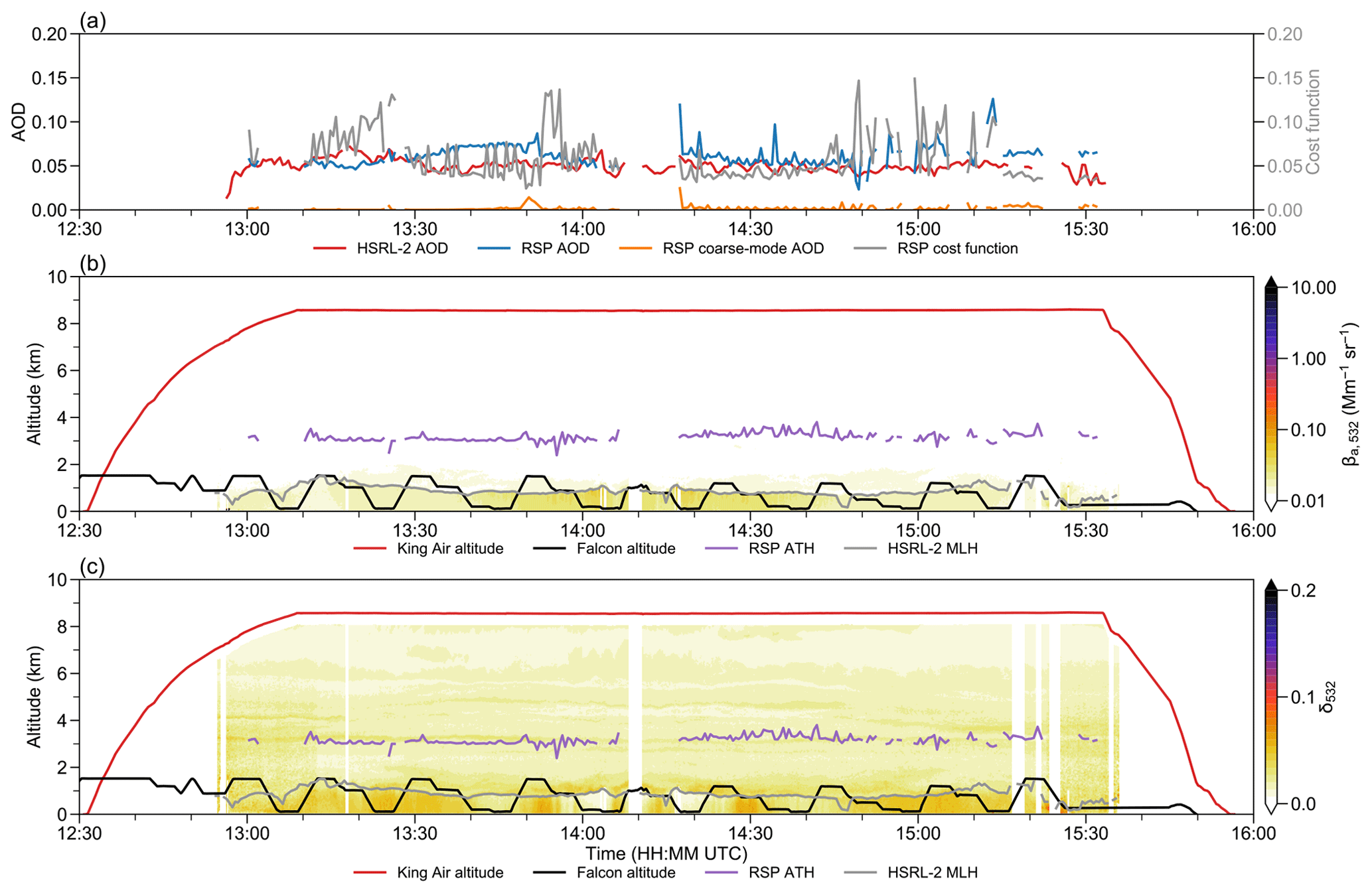
Figure 12Time series of selected measurements during ACTIVATE RF67 on 19 May 2021. (a) HSRL-2 (red), RSP total (blue), RSP coarse-mode (orange) AOD, and RSP normalized cost function (gray). (b)–(c) King Air (red) and Falcon (black) altitude, RSP aerosol top height (purple), and HSRL-2 mixing layer height (gray). All altitude values are in kilometers. (b) HSRL-2 532 nm aerosol scattering coefficient βa,532 in Mm−1 sr−1 (color scale). (c) HSRL-2 532 nm depolarization ratio δ532 (color scale).
The presence of non-spherical aerosols may be indicated by the presence of three HSRL-2 aerosol types: ice, pure dust, and the dusty mix (Fig. 9a). Generally, the linear depolarization ratio is zero for spherical particles but markedly departs from zero for non-spherical particles (Mishchenko and Hovenier, 1995). Therefore, all these aerosol types are characterized by a high degree of aerosol depolarization, although there is not a clear-cut threshold for these three aerosol types. Schlosser et al. (2022) deemed 0.13 a suitable threshold for the maritime study region of ACTIVATE. Burton et al. (2013) found that the first quartiles of depolarization for ice, pure dust, and the dusty mix are 0.23, 0.31, and 0.13, respectively, from measurements collected on 109 flights during 2006 and 2012. The HSRL-2 column-maximum depolarization is more than 0.1 for over 84 % of measurements (Fig. 9d). However, unless the column-maximum depolarization is less than 0.05, all other data groups show a large bias range.
As part of marine aerosols, sea salt is another potential source for contributing to high depolarization in the marine boundary layer due to its shape. Pure dry sea salt is non-spherical, but its shape is sensitive to ambient relative humidity (RH). When RH increases, the sea salt particle remains solid until it reaches the deliquescence RH at which the solid particle absorbs water and forms aqueous solution. The aqueous-phase sea salt is nearly spherical and therefore has low depolarization. On the contrary, when RH decreases, the aqueous sea salt solution can return to its crystalline form at the efflorescence RH. The deliquescence and efflorescence RHs are usually different. Therefore, the shape of a sea salt particle depends not only on the magnitude but also the history of ambient RH (Haarig et al., 2017).
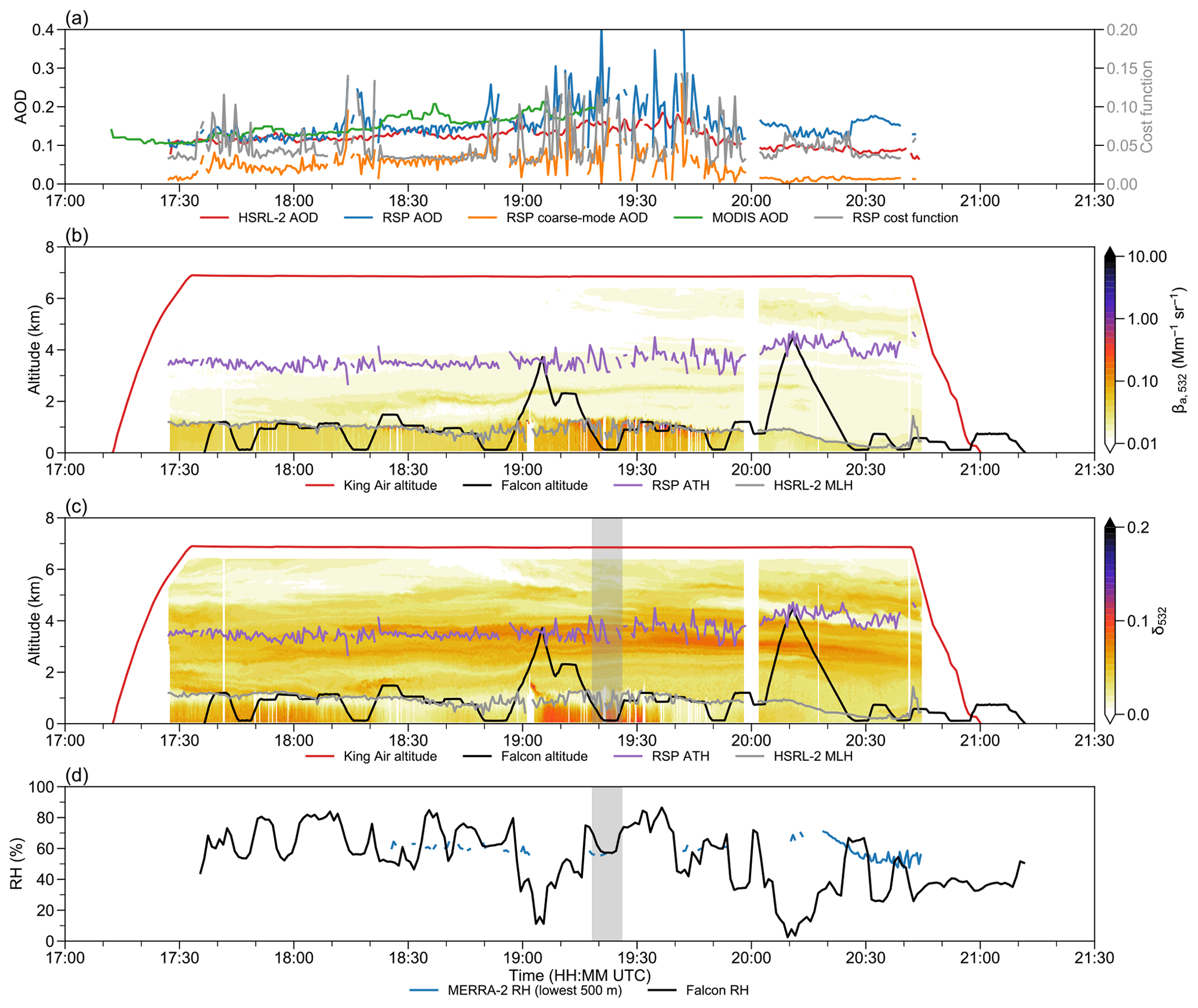
Figure 13Time series of selected measurements during ACTIVATE RF143 on 22 March 2022. (a) HSRL-2 (red), RSP total (blue), RSP coarse-mode (orange), MODIS (green) AOD, and RSP normalized cost function (gray). (b)–(c) King Air (red) and Falcon (black) altitude, RSP aerosol top height (purple), and HSRL-2 mixing layer height (gray). All altitudes are in kilometers. (b) HSRL-2 532 nm aerosol scattering coefficient βa,532 in Mm−1 sr−1 (color scale). (c) HSRL-2 532 nm depolarization ratio δ532 (color scale). (d) Lowest 500 m MERRA-2 (blue) and Falcon (black) relative humidity in percent.
Ferrare et al. (2023) reported that sea salt may cause high depolarization at low RH (i.e., more likely to be non-spherical) within the boundary layer for around one-third of flights during the first 2 years of ACTIVATE based on HSRL-2 and dropsonde measurements. Here we extend the result by collocating the maximum HSRL-2 depolarization at the lowest 500 m with the interpolated MERRA-2 RH for the whole campaign period (Fig. 9e). Seethala et al. (2021) showed that despite having a rather coarse spatial resolution, MERRA-2 adequately reconstructs the observed lower tropospheric thermodynamic structure during ACTIVATE, especially the relative humidity and specific humidity fields. Median depolarization gradually increases when RH decreases, suggesting that sea salt may change its shape over a wide range of RH due to both deliquescence and efflorescence. Note that low RH conditions (<60 %) only occur for around 25 % of time, which means non-spherical aerosols do not often play a big role in the RSP retrieval errors.
The high depolarization associated with sea salt provides evidence of the existence of aerosols close to the surface because sea surface is the major source of sea salt in marine boundary layer. Conversely, it is more difficult to detect aerosols near and above the aircraft. The near-range limit for all ACTIVATE HSRL-2 extinction profiles is 1500 m so that the transmitter-to-receiver overlap function is close to 1 (Burton et al., 2012; Hair et al., 2008). To detect the possibility of aerosols within the near range of aircraft, we compute an effective HSRL-2 aerosol top height ht, which is analogous to the RSP MAPP aerosol top height (Stamnes et al., 2018):
where ht is aerosol top height, h is aircraft altitude, and α is extinction coefficient.
The aerosol top height difference Δht can then be defined as the difference between the aircraft altitude and effective aerosol top height (Fig. 10). Obviously, the difference is at least 1500 m due to the near-range limit (Fig. 9f). A small difference indicates that the aerosol profile is top heavy, but the result for 1500–2000 m does not show larger bias compared to other groups. Note that the dispersion of bias is much smaller when the effective top height is very low.
Aerosols above the aircraft can be estimated from the CALIPSO stratospheric AOD (Fig. 11). Climatologically, the mean stratospheric AOD in the study region is around 0.011 and swings between 0.008 and 0.013 throughout a year. During ACTIVATE, the 2020 winter deployment experienced the record-high AOD in February and March, and the 2021 summer deployment experienced the record-high AOD in May for all CALIPSO years (2006–2021). Major possible sources of stratospheric AOD perturbation in midlatitudes include volcanic eruption and deep convection (Kremser et al., 2016).
We speculate that the large stratospheric AOD perturbations are more likely due to volcanic eruption, not deep convection. First, overshooting convection climatologically occurs more often over land than ocean in midlatitudes (Liu et al., 2020). Second, most of the overshooting convection in the 30–40° latitude band occurs during MAM and JJA (Liu et al., 2020), which is opposite to the CALIPSO climatology, i.e., maxima during SON and DJF but minima during MAM and JJA. The peak AOD in 2020 may be due to the stratospheric eruption at Raikoke (48° N, 153° E) in June 2019 (Kloss et al., 2021). Its estimated plume top height is about 16–17 km from the Himawari-8 satellite. Subsequently the stratospheric AOD increased up to 0.027 in October 2019 (not shown) and gradually decreased in the ensuing months. The spike in May 2021 may be due to the eruption at La Soufrière (13° N, 61° W) in April. Although there are large stratospheric AOD perturbations during ACTIVATE, their magnitude (∼ 0.01–0.02) cannot explain all the biases between the datasets in this study. Therefore, the influence of aerosols above the aircraft should be relatively small compared to other factors.

Figure 14Time series of selected measurements during ACTIVATE RF170 on 10 June 2022. (a) HSRL-2 (red), RSP total (blue), RSP coarse-mode (orange), MODIS (green) AOD, and RSP normalized cost function (gray). (b)–(c) King Air (red) and Falcon (black) altitude, RSP aerosol top height (purple), and HSRL-2 mixing layer height (gray). All altitudes are in kilometers. (b) HSRL-2 532 nm aerosol scattering coefficient βa,532 in Mm−1 sr−1 (color scale). (c) HSRL-2 532 nm depolarization ratio δ532 (color scale). (d) Lowest 500 m MERRA-2 (blue) and Falcon (black) relative humidity in percent.
Other than the single homogeneous aerosol layer assumption, the assumption of coarse-mode sea salt aerosol being located between the surface and 1 km may also lead to retrieval uncertainties. During summer deployments, the mean HSRL-2 mixed layer height (MLH) is around 534 m. The bias is much larger when the RSP coarse-mode aerosol layer height (assumed to be 1 km) is much higher than the HSRL-2 MLH (Fig. 9g). During winter deployments, the mean HSRL-2 MLH (around 764 m) is much closer to the RSP coarse-mode aerosol layer height, but the large bias prevails when there is big mismatch between two heights (Fig. 9h). Note that on average the coarse-mode RSP AOD accounts around 14 % of total RSP AOD so the overall influence is likely to be tiny.
It is beneficial to consolidate the result by revisiting all factors. (i) There is no direct evidence for the presence of above-aircraft aerosols, but elevated stratospheric AOD is seen at least in 2020 and 2021, though the overall impact should be small. (iii) There is no direct evidence for aerosols near aircraft. (ii) and (iv)–(viii) There is evidence for the presence of above-aircraft clouds, clouds surrounding the aircraft, sea salt near the sea surface, more than two aerosol layers, absorbing aerosols, and non-spherical aerosols. (ix) There is evidence for simplified and unwarranted assumptions, but the impact may be small.
4.5 Case studies
Three case studies are arranged to complement the previous analysis. All three cases are statistical surveys in which Falcon collects data at different levels of marine boundary layer. Full details of the Falcon flight strategy and rationale for statistical survey flights are provided in Dadashazar et al. (2022) and Sorooshian et al. (2023).
The first case study is research flight (RF) 67 on 19 May 2021 (King Air: 12:31–15:55 UTC; Falcon: 12:27–15:49 UTC). The two aircraft took off from NASA LaRC, headed southeast via OXANA, and returned near 33° N. RF67 provides a baseline for good agreement between RSP and HSRL-2 AOD. Except near the turning point and towards the end of the trip, the whole survey is mostly cloud free and under light wind.
Generally, the aerosol loading is low, and the difference between RSP and HSRL-2 AOD is small (Fig. 12a). The RSP cost function is small most of the time. The resemblance between RSP and HSRL-2 can be attributed to the relative simple aerosol vertical distribution. Most of the RSP AOD comes from the fine mode (Fig. 12a). The RSP aerosol top height stays at around 3 km (Fig. 12b). The HSRL-2 532 nm backscattering coefficient signal mostly concentrates under the mixing layer at 1 km. Also, in the mixing layer, the 532 nm depolarization ratio is low, indicating a small influence from sea salt (Fig. 12c).
The second case study is RF143 on 22 March 2022 (King Air: 17:12–21:00 UTC; Falcon: 17:36–21:12 UTC). The afternoon flight constitutes the return trip from Bermuda to LaRC. While the morning flight (RF142) from LaRC to Bermuda observes a pronounced aerosol gradient, the afternoon homebound flight (RF143) provides a more complicated aerosol structure.
Overall, the aerosol loading is above the monthly average (Fig. 13a). The RSP aerosol top height is higher compared to RF67 with a coupled aerosol layer above the mixing layer (Fig. 13b). The aerosol layer becomes decoupled around 18:30 UTC. Initially, RSP and HSRL-2 AOD agree with each other, which can also be confirmed by the collocated MODIS data. Starting from 19:00 UTC, enhanced aerosol scattering is observed in the boundary layer for around 45 min (Fig. 13b). At the same time, RSP AOD fluctuates a lot with multiple spikes from its coarse mode (Fig. 13a). The rapidly changing RSP AOD is most likely due to both aerosol layers in the mixing layer and near 4 km aloft. Both layers do have a high depolarization ratio which indicates non-spherical aerosols (Fig. 13c). There are not enough MERRA-2 relativity humidity data collocated with HSRL-2 at the lowest 500 m (Fig. 13d), so we make use of in situ relative humidity observations from Falcon near 19:20 UTC (highlighted in gray shade). The high depolarization ratio coincident with relatively low relative humidity suggests that it might be related to sea salt. The HSRL aerosol classification scheme indicates that the decoupled aerosol layer consists of ice and the dusty mix, which partly explains the observed high depolarization ratio.
The final case study is RF170 on 10 June 2022 (King Air: 11:57–15:35 UTC; Falcon: 12:20–15:37 UTC). By that time, the flight base had moved to Bermuda. The two aircraft took off and headed southwest for a statistical survey.
RSP and HSRL-2 AOD at times diverge from each other (Fig. 14a). The occurrence of extreme differences is mostly associated with spikes in RSP coarse-mode AOD. Most of the backscattering signal is below 2 km (Fig. 14b), and the mixing layer is very shallow (around 500 m). A remarkably high depolarization ratio is seen above the mixing layer near 13:45 UTC (Fig. 14c). The high MERRA-2 and Falcon near-surface relative humidity indicates that it is not associated with sea salt (Fig. 14d). The HSRL aerosol classification scheme identifies that most of the high depolarization aerosols between 13:00 and 14:30 UTC consist of a dusty mix, suggesting some seasonal influence from African dusts.
In short, the RSP and HSRL-2 show good agreement in relatively clean environments in the first case study, but as demonstrated by the second and third cases, the RSP retrieval degrades under a high polarization ratio, which indicates the influence of non-spherical aerosols.
We analyzed 3 years of AOD data over the western North Atlantic Ocean and attempted to estimate and understand their uncertainties, using two retrieval products collected during ACTIVATE and one satellite retrieval product. The key findings are as follows:
-
RSP and HSRL-2 AOD have large seasonal variations but also exhibit considerable deviations between the two retrievals. The absence of a reference dataset over the western North Atlantic Ocean, and arguably all global marine areas, prompts us to use triple collocation to determine which dataset is more accurate.
-
Triple collocation analysis indicates that HSRL-2 is the most accurate dataset over the study region. The correlation coefficient and error standard deviation of AOD with respect to the expected ground truth are 0.93 and 0.027, respectively.
-
The RSP retrieval quality can be improved considerably by applying a simple, yet efficient, filtering criterion: a more stringent normalized cost function of 0.05. There are two additional benefits. First, it can be easily applied globally. Second, it is suitable for offline post-processing.
-
The reasons of disagreement between RSP and HSRL-2 are statistically diagnosed using all ACTIVATE datasets. There is a basket of potential factors, including cloud contamination, aerosols near the surface, multiple aerosol layers, absorbing aerosols, non-spherical aerosols, and simplified retrieval assumptions. The statistical analysis is accompanied with case studies of both subpar and high-quality RSP retrievals. By combining information from lidar, polarimeter, and other pertinent datasets, it is possible to single out the most probable causes of poor retrievals, such that RSP AOD retrievals can be optimally improved.
Motivated by the last point, future efforts are needed along two lines: multi-angle polarimeter and HSRL (or HSRL-2) data from other field campaigns should be analyzed to test the robustness of the conclusions here, and a more efficient retrieval of HSRL-2 MLH data should be developed potentially through two-dimensional image processing. Earlier recommendations such as combining HSRL-2 elevated aerosol layer altitudes with RSP retrievals should be reconsidered (Knobelspiesse et al., 2011). The current HSRL-2 MLH retrieval algorithm detects the edge of aerosol gradient in each one-dimensional column. Instead, reading the whole two-dimensional flight curtain at once and using a two-dimensional wavelet transform will potentially speed up the computation and improve the detection accuracy. The above results will provide a better constraint on aerosol properties and help prepare concurrent deployments of lidars and polarimeters for future spaceborne missions.
All the data used in this work are publicly available. The ACTIVATE data can be downloaded from https://doi.org/10.5067/SUBORBITAL/ACTIVATE/DATA001 (NASA/LARC/SD/ASDC, 2021). The MODIS Terra and Aqua data can be downloaded from https://doi.org/10.5067/MODIS/MOD04_3K.061 (MODIS Science Team, 2017a) and https://doi.org/10.5067/MODIS/MYD04_3K.061 (MODIS Science Team, 2017b). The CALIPSO data can be downloaded from 10.5067/CALIOP/CALIPSO/LID_L3 (NASA/LARC/SD/ASDC, 2018) and 10.5067/CALIOP/CALIPSO/CAL_LID_L3 (NASA/LARC/SD/ASDC, 2020).
The supplement related to this article is available online at: https://doi.org/10.5194/amt-17-2739-2024-supplement.
All authors contributed to preparation of the manuscript. Conceptualization: LWS, JSS, and DP. Methodology: LWS, JSS, DP, and LL. Funding acquisition and resources: AS, JWH, RAF, and XZ. Project administration: MK. Supervision: AS and XZ. Writing (original draft preparation): LWS. Data curation, formal analysis, investigation, software, validation, visualization, and writing (review and editing): LWS, JSS, DP, BC, MAF, RAF, JWH, CAH, LL, MMK, AJS, TS, AS, SS, and XZ.
The contact author has declared that none of the authors has any competing interests.
Publisher’s note: Copernicus Publications remains neutral with regard to jurisdictional claims made in the text, published maps, institutional affiliations, or any other geographical representation in this paper. While Copernicus Publications makes every effort to include appropriate place names, the final responsibility lies with the authors.
This article is part of the special issue “Marine aerosols, trace gases, and clouds over the North Atlantic (ACP/AMT inter-journal SI)”. It is not associated with a conference.
We thank the pilots and aircraft maintenance personnel of NASA Langley Research Services Directorate for their work in conducting the ACTIVATE flights. We are appreciative of the editor and two anonymous reviewers for their insightful comments that improved the manuscript. This work is supported by NASA grant 80NSSC19K0442 for ACTIVATE, a NASA Earth Venture Suborbital-3 (EVS-3) investigation, which is funded by NASA’s Earth Science Division and managed through the Earth System Science Pathfinder Program Office.
This research has been supported by the National Aeronautics and Space Administration (grant no. 80NSSC19K0442).
This paper was edited by Roger Marchand and reviewed by two anonymous referees.
Aldhaif, A. M., Lopez, D. H., Dadashazar, H., and Sorooshian, A.: Sources, frequency, and chemical nature of dust events impacting the United States East Coast, Atmos. Environ., 231, 117456, https://doi.org/10.1016/j.atmosenv.2020.117456, 2020. a
Alexandrov, M. D., Cairns, B., Emde, C., Ackerman, A. S., and van Diedenhoven, B.: Accuracy assessments of cloud droplet size retrievals from polarized reflectance measurements by the Research Scanning Polarimeter, Remote Sens. Environ., 125, 92–111, https://doi.org/10.1016/j.rse.2012.07.012, 2012. a, b
Anderson, T. L., Charlson, R. J., Winker, D. M., Ogren, J. A., and Holmén, K.: Mesoscale variations of tropospheric aerosols, J. Atmos. Sci., 60, 119–136, https://doi.org/10.1175/1520-0469(2003)060<0119:mvota>2.0.co;2, 2003. a, b, c, d
Andreae, M. O.: Correlation between cloud condensation nuclei concentration and aerosol optical thickness in remote and polluted regions, Atmos. Chem. Phys., 9, 543–556, https://doi.org/10.5194/acp-9-543-2009, 2009. a
Antuña-Marrero, J. C., Cachorro Revilla, V., García Parrado, F., de Frutos Baraja, Á., Rodríguez Vega, A., Mateos, D., Estevan Arredondo, R., and Toledano, C.: Comparison of aerosol optical depth from satellite (MODIS), sun photometer and broadband pyrheliometer ground-based observations in Cuba, Atmos. Meas. Tech., 11, 2279–2293, https://doi.org/10.5194/amt-11-2279-2018, 2018. a, b
Bellouin, N., Quaas, J., Gryspeerdt, E., Kinne, S., Stier, P., Watson-Parris, D., Boucher, O., Carslaw, K. S., Christensen, M., Daniau, A.-L., Dufresne, J.-L., Feingold, G., Fiedler, S., Forster, P., Gettelman, A., Haywood, J. M., Lohmann, U., Malavelle, F., Mauritsen, T., McCoy, D. T., Myhre, G., Mülmenstädt, J., Neubauer, D., Possner, A., Rugenstein, M., Sato, Y., Schulz, M., Schwartz, S. E., Sourdeval, O., Storelvmo, T., Toll, V., Winker, D., and Stevens, B.: Bounding global aerosol radiative forcing of climate change, Rev. Geophys., 58, 117456, https://doi.org/10.1029/2019rg000660, 2020. a
Burton, S. P., Ferrare, R. A., Hostetler, C. A., Hair, J. W., Rogers, R. R., Obland, M. D., Butler, C. F., Cook, A. L., Harper, D. B., and Froyd, K. D.: Aerosol classification using airborne High Spectral Resolution Lidar measurements – methodology and examples, Atmos. Meas. Tech., 5, 73–98, https://doi.org/10.5194/amt-5-73-2012, 2012. a, b, c
Burton, S. P., Ferrare, R. A., Vaughan, M. A., Omar, A. H., Rogers, R. R., Hostetler, C. A., and Hair, J. W.: Aerosol classification from airborne HSRL and comparisons with the CALIPSO vertical feature mask, Atmos. Meas. Tech., 6, 1397–1412, https://doi.org/10.5194/amt-6-1397-2013, 2013. a, b
Burton, S. P., Chemyakin, E., Liu, X., Knobelspiesse, K., Stamnes, S., Sawamura, P., Moore, R. H., Hostetler, C. A., and Ferrare, R. A.: Information content and sensitivity of the 3β + 2α lidar measurement system for aerosol microphysical retrievals, Atmos. Meas. Tech., 9, 5555–5574, https://doi.org/10.5194/amt-9-5555-2016, 2016. a
Burton, S. P., Hostetler, C. A., Cook, A. L., Hair, J. W., Seaman, S. T., Scola, S., Harper, D. B., Smith, J. A., Fenn, M. A., Ferrare, R. A., Saide, P. E., Chemyakin, E. V., and Müller, D.: Calibration of a high spectral resolution lidar using a Michelson interferometer, with data examples from ORACLES, Appl. Opt., 57, 6061, https://doi.org/10.1364/ao.57.006061, 2018. a
Caires, S. and Sterl, A.: Validation of ocean wind and wave data using triple collocation, J. Geophys. Res., 108, 3098, https://doi.org/10.1029/2002jc001491, 2003. a, b
Cairns, B., Russell, E. E., and Travis, L. D.: Research Scanning Polarimeter: calibration and ground-based measurements, in: Proceedings of SPIE, edited by: Goldstein, D. H. and Chenault, D. B., Vol. 3754, 186–196, SPIE, https://doi.org/10.1117/12.366329, 1999. a
Cairns, B., Russell, E. E., LaVeigne, J. D., and Tennant, P. M. W.: Research Scanning Polarimeter and airborne usage for remote sensing of aerosols, in: Proceedings of SPIE, edited by: Shaw, J. A. and Tyo, J. S., Vol. 5158, 33–44, SPIE, https://doi.org/10.1117/12.518320, 2003. a, b
Chen, Y.-C., Christensen, M. W., Stephens, G. L., and Seinfeld, J. H.: Satellite-based estimate of global aerosol–cloud radiative forcing by marine warm clouds, Nat. Geosci., 7, 643–646, https://doi.org/10.1038/ngeo2214, 2014. a
Chylek, P., Henderson, B., and Mishchenko, M.: Aerosol radiative forcing and the accuracy of satellite aerosol optical depth retrieval, J. Geophys. Res.-Atmos., 108, 1–8, https://doi.org/10.1029/2003jd004044, 2003. a
Corral, A. F., Braun, R. A., Cairns, B., Gorooh, V. A., Liu, H., Ma, L., Mardi, A. H., Painemal, D., Stamnes, S., van Diedenhoven, B., Wang, H., Yang, Y., Zhang, B., and Sorooshian, A.: An overview of atmospheric features over the Western North Atlantic Ocean and North American East Coast – Part 1: Analysis of aerosols, gases, and wet deposition chemistry, J. Geophys. Res.-Atmos., 126, e2020JD32592, https://doi.org/10.1029/2020jd032592, 2021. a
Dadashazar, H., Crosbie, E., Choi, Y., Corral, A. F., DiGangi, J. P., Diskin, G. S., Dmitrovic, S., Kirschler, S., McCauley, K., Moore, R. H., Nowak, J. B., Robinson, C. E., Schlosser, J., Shook, M., Thornhill, K. L., Voigt, C., Winstead, E. L., Ziemba, L. D., and Sorooshian, A.: Analysis of MONARC and ACTIVATE airborne aerosol data for aerosol-cloud interaction investigations: Efficacy of stairstepping flight legs for airborne in situ sampling, Atmosphere, 13, 1242, https://doi.org/10.3390/atmos13081242, 2022. a
Di Noia, A., Hasekamp, O. P., Wu, L., van Diedenhoven, B., Cairns, B., and Yorks, J. E.: Combined neural network/Phillips–Tikhonov approach to aerosol retrievals over land from the NASA Research Scanning Polarimeter, Atmos. Meas. Tech., 10, 4235–4252, https://doi.org/10.5194/amt-10-4235-2017, 2017. a
Diskin, G. S., Podolske, J. R., Sachse, G. W., and Slate, T. A.: Open-path airborne tunable diode laser hygrometer, in: Diode Lasers and Applications in Atmospheric Sensing, edited by: Fried, A., SPIE, ISSN 0277-786X, https://doi.org/10.1117/12.453736, 2002. a
Draper, C., Reichle, R., de Jeu, R., Naeimi, V., Parinussa, R., and Wagner, W.: Estimating root mean square errors in remotely sensed soil moisture over continental scale domains, Remote Sens. Environ., 137, 288–298, https://doi.org/10.1016/j.rse.2013.06.013, 2013. a
Ferrare, R., Hair, J., Hostetler, C., Shingler, T., Burton, S. P., Fenn, M., Clayton, M., Scarino, A. J., Harper, D., Seaman, S., Cook, A., Crosbie, E., Winstead, E., Ziemba, L., Thornhill, L., Robinson, C., Moore, R., Vaughan, M., Sorooshian, A., Schlosser, J. S., Liu, H., Zhang, B., Diskin, G., DiGangi, J., Nowak, J., Choi, Y., Zuidema, P., and Chellappan, S.: Airborne HSRL-2 measurements of elevated aerosol depolarization associated with non-spherical sea salt, Front. Remote Sens., 4, 1–18, https://doi.org/10.3389/frsen.2023.1143944, 2023. a, b, c
Fu, G., Hasekamp, O., Rietjens, J., Smit, M., Di Noia, A., Cairns, B., Wasilewski, A., Diner, D., Seidel, F., Xu, F., Knobelspiesse, K., Gao, M., da Silva, A., Burton, S., Hostetler, C., Hair, J., and Ferrare, R.: Aerosol retrievals from different polarimeters during the ACEPOL campaign using a common retrieval algorithm, Atmos. Meas. Tech., 13, 553–573, https://doi.org/10.5194/amt-13-553-2020, 2020. a
Gao, M., Knobelspiesse, K., Franz, B. A., Zhai, P.-W., Sayer, A. M., Ibrahim, A., Cairns, B., Hasekamp, O., Hu, Y., Martins, V., Werdell, P. J., and Xu, X.: Effective uncertainty quantification for multi-angle polarimetric aerosol remote sensing over ocean, Atmos. Meas. Tech., 15, 4859–4879, https://doi.org/10.5194/amt-15-4859-2022, 2022. a, b
Gauch, H. G., Hwang, J. T. G., and Fick, G. W.: Model evaluation by comparison of model-based predictions and measured values, Agronomy J., 95, 1442–1446, https://doi.org/10.2134/agronj2003.1442, 2003. a
Gelaro, R., McCarty, W., Suárez, M. J., Todling, R., Molod, A., Takacs, L., Randles, C. A., Darmenov, A., Bosilovich, M. G., Reichle, R., Wargan, K., Coy, L., Cullather, R., Draper, C., Akella, S., Buchard, V., Conaty, A., da Silva, A. M., Gu, W., Kim, G.-K., Koster, R., Lucchesi, R., Merkova, D., Nielsen, J. E., Partyka, G., Pawson, S., Putman, W., Rienecker, M., Schubert, S. D., Sienkiewicz, M., and Zhao, B.: The Modern-Era Retrospective Analysis for Research and Applications, version 2 (MERRA-2), J. Climate, 30, 5419–5454, https://doi.org/10.1175/JCLI-D-16-0758.1, 2017. a
Gruber, A., Su, C.-H., Zwieback, S., Crow, W., Dorigo, W., and Wagner, W.: Recent advances in (soil moisture) triple collocation analysis, Int. J. Appl. Earth Observ. Geoinfo., 45, 200–211, https://doi.org/10.1016/j.jag.2015.09.002, 2016. a
Haarig, M., Ansmann, A., Gasteiger, J., Kandler, K., Althausen, D., Baars, H., Radenz, M., and Farrell, D. A.: Dry versus wet marine particle optical properties: RH dependence of depolarization ratio, backscatter, and extinction from multiwavelength lidar measurements during SALTRACE, Atmos. Chem. Phys., 17, 14199–14217, https://doi.org/10.5194/acp-17-14199-2017, 2017. a
Hair, J. W., Hostetler, C. A., Cook, A. L., Harper, D. B., Ferrare, R. A., Mack, T. L., Welch, W., Izquierdo, L. R., and Hovis, F. E.: Airborne High Spectral Resolution Lidar for profiling aerosol optical properties, Appl. Opt., 47, 6734, https://doi.org/10.1364/ao.47.006734, 2008. a, b, c
Hansen, J., Rossow, W., Carlson, B., Lacis, A., Travis, L., Del Genio, A., Fung, I., Cairns, B., Mishchenko, M., and Sato, M.: Low-cost long-term monitoring of global climate forcings and feedbacks, Clim. Change, 31, 247–271, https://doi.org/10.1007/BF01095149, 1995. a
Holben, B., Eck, T., Slutsker, I., Tanré, D., Buis, J., Setzer, A., Vermote, E., Reagan, J., Kaufman, Y., Nakajima, T., Lavenu, F., Jankowiak, I., and Smirnov, A.: AERONET – A federated instrument network and data archive for aerosol characterization, Remote Sens. Environ., 66, 1–16, https://doi.org/10.1016/S0034-4257(98)00031-5, 1998. a
IPCC: Climate Change 2021: The Physical Science Basis. Contribution of Working Group I to the Sixth Assessment Report of the Intergovernmental Panel on Climate Change, Cambridge University Press, Cambridge, United Kingdom, https://doi.org/10.1017/9781009157896, 2023. a
Janssen, P. A. E. M., Abdalla, S., Hersbach, H., and Bidlot, J.-R.: Error estimation of buoy, satellite, and model wave height data, J. Atmos. Ocean. Technol., 24, 1665–1677, https://doi.org/10.1175/jtech2069.1, 2007. a
Kar, J., Lee, K.-P., Vaughan, M. A., Tackett, J. L., Trepte, C. R., Winker, D. M., Lucker, P. L., and Getzewich, B. J.: CALIPSO level 3 stratospheric aerosol profile product: version 1.00 algorithm description and initial assessment, Atmos. Meas. Tech., 12, 6173–6191, https://doi.org/10.5194/amt-12-6173-2019, 2019. a
Kloss, C., Berthet, G., Sellitto, P., Ploeger, F., Taha, G., Tidiga, M., Eremenko, M., Bossolasco, A., Jégou, F., Renard, J.-B., and Legras, B.: Stratospheric aerosol layer perturbation caused by the 2019 Raikoke and Ulawun eruptions and their radiative forcing, Atmos. Chem. Phys., 21, 535–560, https://doi.org/10.5194/acp-21-535-2021, 2021. a
Knobelspiesse, K., Cairns, B., Ottaviani, M., Ferrare, R., Hair, J., Hostetler, C., Obland, M., Rogers, R., Redemann, J., Shinozuka, Y., Clarke, A., Freitag, S., Howell, S., Kapustin, V., and McNaughton, C.: Combined retrievals of boreal forest fire aerosol properties with a polarimeter and lidar, Atmospheric Chemistry and Physics, 11, 7045–7067, https://doi.org/10.5194/acp-11-7045-2011, 2011. a, b
Kremser, S., Thomason, L. W., von Hobe, M., Hermann, M., Deshler, T., Timmreck, C., Toohey, M., Stenke, A., Schwarz, J. P., Weigel, R., Fueglistaler, S., Prata, F. J., Vernier, J.-P., Schlager, H., Barnes, J. E., Antuña-Marrero, J.-C., Fairlie, D., Palm, M., Mahieu, E., Notholt, J., Rex, M., Bingen, C., Vanhellemont, F., Bourassa, A., Plane, J. M. C., Klocke, D., Carn, S. A., Clarisse, L., Trickl, T., Neely, R., James, A. D., Rieger, L., Wilson, J. C., and Meland, B.: Stratospheric aerosol–Observations, processes, and impact on climate, Rev. Geophys., 54, 278–335, https://doi.org/10.1002/2015rg000511, 2016. a
Levy, R. C., Mattoo, S., Munchak, L. A., Remer, L. A., Sayer, A. M., Patadia, F., and Hsu, N. C.: The Collection 6 MODIS aerosol products over land and ocean, Atmos. Meas. Tech., 6, 2989–3034, https://doi.org/10.5194/amt-6-2989-2013, 2013. a, b, c
Liu, N., Liu, C., and Hayden, L.: Climatology and detection of overshooting convection from 4 years of GPM precipitation radar and passive microwave observations, J. Geophys. Res.-Atmos., 125, e2019JD032003, https://doi.org/10.1029/2019jd032003, 2020. a, b
Lohmann, U. and Feichter, J.: Global indirect aerosol effects: a review, Atmos. Chem. Phys., 5, 715–737, https://doi.org/10.5194/acp-5-715-2005, 2005. a
Mardi, A. H., Dadashazar, H., Painemal, D., Shingler, T., Seaman, S. T., Fenn, M. A., Hostetler, C. A., and Sorooshian, A.: Biomass burning over the United States East Coast and western North Atlantic Ocean: Implications for clouds and air quality, J. Geophys. Res.-Atmos., 126, e2021JD034916, https://doi.org/10.1029/2021jd034916, 2021. a
McColl, K. A., Vogelzang, J., Konings, A. G., Entekhabi, D., Piles, M., and Stoffelen, A.: Extended triple collocation: Estimating errors and correlation coefficients with respect to an unknown target, Geophys. Res. Lett., 41, 6229–6236, https://doi.org/10.1002/2014gl061322, 2014. a, b, c
Mishchenko, M. I. and Hovenier, J. W.: Depolarization of light backscattered by randomly oriented nonspherical particles, Opt. Lett., 20, 1356, https://doi.org/10.1364/ol.20.001356, 1995. a
Mishchenko, M. I., Cairns, B., Hansen, J. E., Travis, L. D., Burg, R., Kaufman, Y. J., Vanderlei Martins, J., and Shettle, E. P.: Monitoring of aerosol forcing of climate from space: Analysis of measurement requirements, J. Quant. Spectrosc. Ra., 88, 149–161, https://doi.org/10.1016/j.jqsrt.2004.03.030, 2004. a
MODIS Science Team: MODIS/Terra Aerosol 5-Min L2 Swath 3 km, EarthData [data set], https://doi.org/10.5067/MODIS/MOD04_3K.061, 2017a. a
MODIS Science Team: MODIS/Aqua Aerosol 5-Min L2 Swath 3 km, EarthData [data set], https://doi.org/10.5067/MODIS/MYD04_3K.061, 2017b. a
NASA/LARC/SD/ASDC: CALIPSO Lidar Level 3 Stratospheric Aerosol Profiles Standard V1-00, EarthData [data set], 10.5067/CALIOP/CALIPSO/LID_L3, 2018. a
NASA/LARC/SD/ASDC: CALIPSO Lidar Level 3 Stratospheric Aerosol Profiles Standard V1-01, EarthData [data set], 10.5067/CALIOP/CALIPSO/CAL_LID_L3, 2020. a
NASA/LARC/SD/ASDC: Aerosol Cloud meTeorology Interactions oVer the western ATlantic Experiment (ACTIVATE), EarthData [data set], https://doi.org/10.5067/SUBORBITAL/ACTIVATE/DATA001, 2021. a
Nied, J., Jones, M., Seaman, S., Shingler, T., Hair, J., Cairns, B., Gilst, D. V., Bucholtz, A., Schmidt, S., Chellappan, S., Zuidema, P., Diedenhoven, B. V., Sorooshian, A., and Stamnes, S.: A cloud detection neural network for above-aircraft clouds using airborne cameras, Front. Remote Sens. 4, 1118745, https://doi.org/10.3389/frsen.2023.1118745, 2023. a
O'Carroll, A. G., Eyre, J. R., and Saunders, R. W.: Three-way error analysis between AATSR, AMSR-E, and in situ sea surface temperature observations, J. Atmos. Ocean. Technol., 25, 1197–1207, https://doi.org/10.1175/2007jtecho542.1, 2008. a
Pöschl, U.: Atmospheric aerosols: Composition, transformation, climate and health effects, Angewandte Chemie International Edition, 44, 7520–7540, https://doi.org/10.1002/anie.200501122, 2005. a
Remer, L. A., Kaufman, Y. J., Tanré, D., Mattoo, S., Chu, D. A., Martins, J. V., Li, R.-R., Ichoku, C., Levy, R. C., Kleidman, R. G., Eck, T. F., Vermote, E., and Holben, B. N.: The MODIS aerosol algorithm, products, and validation, J. Atmos. Sci., 62, 947–973, https://doi.org/10.1175/jas3385.1, 2005. a, b
Remer, L. A., Mattoo, S., Levy, R. C., and Munchak, L. A.: MODIS 3 km aerosol product: algorithm and global perspective, Atmos. Meas. Tech., 6, 1829–1844, https://doi.org/10.5194/amt-6-1829-2013, 2013. a, b, c
Rodgers, C. D.: Inverse Methods for Atmospheric Sounding: Theory and Practice, World Scientific, Singapore, https://doi.org/10.1142/3171, 2000. a
Sawamura, P., Moore, R. H., Burton, S. P., Chemyakin, E., Müller, D., Kolgotin, A., Ferrare, R. A., Hostetler, C. A., Ziemba, L. D., Beyersdorf, A. J., and Anderson, B. E.: HSRL-2 aerosol optical measurements and microphysical retrievals vs. airborne in situ measurements during DISCOVER-AQ 2013: an intercomparison study, Atmos. Chem. Phys., 17, 7229–7243, https://doi.org/10.5194/acp-17-7229-2017, 2017. a
Sayer, A. M., Govaerts, Y., Kolmonen, P., Lipponen, A., Luffarelli, M., Mielonen, T., Patadia, F., Popp, T., Povey, A. C., Stebel, K., and Witek, M. L.: A review and framework for the evaluation of pixel-level uncertainty estimates in satellite aerosol remote sensing, Atmos. Meas. Tech., 13, 373–404, https://doi.org/10.5194/amt-13-373-2020, 2020. a
Scarino, A. J., Obland, M. D., Fast, J. D., Burton, S. P., Ferrare, R. A., Hostetler, C. A., Berg, L. K., Lefer, B., Haman, C., Hair, J. W., Rogers, R. R., Butler, C., Cook, A. L., and Harper, D. B.: Comparison of mixed layer heights from airborne high spectral resolution lidar, ground-based measurements, and the WRF-Chem model during CalNex and CARES, Atmos. Chem. Phys., 14, 5547–5560, https://doi.org/10.5194/acp-14-5547-2014, 2014. a
Schlosser, J. S., Stamnes, S., Burton, S. P., Cairns, B., Crosbie, E., Van Diedenhoven, B., Diskin, G., Dmitrovic, S., Ferrare, R., Hair, J. W., Hostetler, C. A., Hu, Y., Liu, X., Moore, R. H., Shingler, T., Shook, M. A., Thornhill, K. L., Winstead, E., Ziemba, L., and Sorooshian, A.: Polarimeter + lidar–derived aerosol particle number concentration, Front. Remote Sens., 3, 1–13, https://doi.org/10.3389/frsen.2022.885332, 2022. a, b, c, d
Seethala, C., Zuidema, P., Edson, J., Brunke, M., Chen, G., Li, X.-Y., Painemal, D., Robinson, C., Shingler, T., Shook, M., Sorooshian, A., Thornhill, L., Tornow, F., Wang, H., Zeng, X., and Ziemba, L.: On assessing ERA5 and MERRA2 representations of cold-air outbreaks across the Gulf Stream, Geophys. Res. Lett., 48, e2021GL094364, https://doi.org/10.1029/2021gl094364, 2021. a
Seinfeld, J. H., Bretherton, C., Carslaw, K. S., Coe, H., DeMott, P. J., Dunlea, E. J., Feingold, G., Ghan, S., Guenther, A. B., Kahn, R., Kraucunas, I., Kreidenweis, S. M., Molina, M. J., Nenes, A., Penner, J. E., Prather, K. A., Ramanathan, V., Ramaswamy, V., Rasch, P. J., Ravishankara, A. R., Rosenfeld, D., Stephens, G., and Wood, R.: Improving our fundamental understanding of the role of aerosol-cloud interactions in the climate system, P. Natl. Acad. Sci. USA, 113, 5781–5790, https://doi.org/10.1073/pnas.1514043113, 2016. a
Shinozuka, Y., Johnson, R. R., Flynn, C. J., Russell, P. B., Schmid, B., Redemann, J., Dunagan, S. E., Kluzek, C. D., Hubbe, J. M., Segal-Rosenheimer, M., Livingston, J. M., Eck, T. F., Wagener, R., Gregory, L., Chand, D., Berg, L. K., Rogers, R. R., Ferrare, R. A., Hair, J. W., Hostetler, C. A., and Burton, S. P.: Hyperspectral aerosol optical depths from TCAP flights, J. Geophys. Res.-Atmos., 118, 12,180–12,194, https://doi.org/10.1002/2013jd020596, 2013. a
Sorooshian, A., Anderson, B., Bauer, S. E., Braun, R. A., Cairns, B., Crosbie, E., Dadashazar, H., Diskin, G., Ferrare, R., Flagan, R. C., Hair, J., Hostetler, C., Jonsson, H. H., Kleb, M. M., Liu, H., MacDonald, A. B., McComiskey, A., Moore, R., Painemal, D., Russell, L. M., Seinfeld, J. H., Shook, M., Smith, W. L., Thornhill, K., Tselioudis, G., Wang, H., Zeng, X., Zhang, B., Ziemba, L., and Zuidema, P.: Aerosol–cloud–meteorology interaction airborne field investigations: Using lessons learned from the U.S. West Coast in the design of ACTIVATE off the U.S. East Coast, B. Am. Meteorol. Soc., 100, 1511–1528, https://doi.org/10.1175/bams-d-18-0100.1, 2019. a, b
Sorooshian, A., Alexandrov, M. D., Bell, A. D., Bennett, R., Betito, G., Burton, S. P., Buzanowicz, M. E., Cairns, B., Chemyakin, E. V., Chen, G., Choi, Y., Collister, B. L., Cook, A. L., Corral, A. F., Crosbie, E. C., van Diedenhoven, B., DiGangi, J. P., Diskin, G. S., Dmitrovic, S., Edwards, E.-L., Fenn, M. A., Ferrare, R. A., van Gilst, D., Hair, J. W., Harper, D. B., Hilario, M. R. A., Hostetler, C. A., Jester, N., Jones, M., Kirschler, S., Kleb, M. M., Kusterer, J. M., Leavor, S., Lee, J. W., Liu, H., McCauley, K., Moore, R. H., Nied, J., Notari, A., Nowak, J. B., Painemal, D., Phillips, K. E., Robinson, C. E., Scarino, A. J., Schlosser, J. S., Seaman, S. T., Seethala, C., Shingler, T. J., Shook, M. A., Sinclair, K. A., Smith Jr., W. L., Spangenberg, D. A., Stamnes, S. A., Thornhill, K. L., Voigt, C., Vömel, H., Wasilewski, A. P., Wang, H., Winstead, E. L., Zeider, K., Zeng, X., Zhang, B., Ziemba, L. D., and Zuidema, P.: Spatially coordinated airborne data and complementary products for aerosol, gas, cloud, and meteorological studies: the NASA ACTIVATE dataset , Earth Syst. Sci. Data, 15, 3419–3472, https://doi.org/10.5194/essd-15-3419-2023, 2023. a, b, c, d, e, f
Stamnes, S., Hostetler, C., Ferrare, R., Burton, S., Liu, X., Hair, J., Hu, Y., Wasilewski, A., Martin, W., van Diedenhoven, B., Chowdhary, J., Cetinić, I., Berg, L. K., Stamnes, K., and Cairns, B.: Simultaneous polarimeter retrievals of microphysical aerosol and ocean color parameters from the “MAPP” algorithm with comparison to high-spectral-resolution lidar aerosol and ocean products, Appl. Opt., 57, 2394, https://doi.org/10.1364/ao.57.002394, 2018. a, b, c, d, e, f, g, h, i
Stoffelen, A.: Toward the true near-surface wind speed: Error modeling and calibration using triple collocation, J. Geophys. Res.-Oceans, 103, 7755–7766, https://doi.org/10.1029/97jc03180, 1998. a, b, c
Winker, D. M., Vaughan, M. A., Omar, A., Hu, Y., Powell, K. A., Liu, Z., Hunt, W. H., and Young, S. A.: Overview of the CALIPSO mission and CALIOP data processing algorithms, J. Atmos. Ocean. Technol., 26, 2310–2323, https://doi.org/10.1175/2009jtecha1281.1, 2009. a
Zwieback, S., Scipal, K., Dorigo, W., and Wagner, W.: Structural and statistical properties of the collocation technique for error characterization, Nonlin. Processes Geophys., 19, 69–80, https://doi.org/10.5194/npg-19-69-2012, 2012. a, b