Evaluation of calibration performance of a low-cost particulate matter sensor using collocated and distant NO₂

Low-cost optical particle sensors have the potential to supplement existing particulate matter (PM) monitoring systems and to provide high spatial and temporal resolutions. However, low-cost PM sensors have often shown questionable performance under various ambient conditions. Temperature, relative humidity (RH), and particle composition have been identified as factors that directly affect the performance of low-cost PM sensors. This study investigated whether NO₂, which creates PM_2.5 by means of chemical reactions in the atmosphere, can be used to improve the calibration performance of low-cost PM_2.5 sensors. To this end, we evaluated the PurpleAir PA-II, called PA-II, a popular air monitoring system that utilizes two low-cost PM sensors and that is frequently deployed near air quality monitoring sites of the Environmental Protection Agency (EPA). We selected a single location where 14 PA-II units have operated for more than 2 years, since July 2017. Based on the operating periods of the PA-II units, we then chose the period of January 2018 to December 2019 for study. Among the 14 units, a single unit containing more than 23 months of measurement data with a high correlation between the unit's two PMS sensors was selected for analysis. Daily and hourly PM_2.5 measurement data from the PA-II unit and a BAM 1020 instrument, respectively, were compared using the federal reference method (FRM), and a per-month analysis was conducted against the BAM-1020 using hourly PM_2.5 data. In the per-month analysis, three key features – namely temperature, relative humidity (RH), and NO₂ – were considered. The NO₂, called collocated NO₂, was collected from the reliable instrument collocated with the PA-II unit. The per-month analysis showed that the PA-II unit had a good correlation (coefficient of determination R²>0.819) with the BAM-1020 during the months of November, December, and January in both 2018 and 2019, but their correlation intensity was moderate during other months, such as in July and September 2018 and August, September, and October 2019. NO₂ was shown to be a key factor in increasing the value of R² in the months when moderate correlation based on only PM_2.5 was achieved. This study calibrated a PA-II unit using multiple linear regression (MLR) and random forest (RF) methods based on the same three features used in the analysis studies, as well as their multiplicative terms. The addition of NO₂ had a much larger effect than that of RH when both PM_2.5 and temperature were considered for calibration in both models. When NO₂, temperature, and relative humidity were considered, the MLR method achieved similar calibration performance to the RF method. In addressing the feasibility of utilizing distant NO₂ measurements for calibration in lieu of collocated data, the study highlights the effectiveness of distant NO₂ when correlated strongly with collocated measurements. This finding offers a practical solution for situations where obtaining collocated NO₂ data proves to be challenging or costly. We assessed the performance of different PA-II units to determine their efficacy. Our investigation reveals a significant enhancement in calibration performance across different PA-II units upon integrating NO₂. Importantly, this improvement remains consistent even when employing models trained with different PA-II units within the same location. Overall, this investigation emphasizes the significance of NO₂ in improving calibration for low-cost PM_2.5 sensors and presents insights into leveraging distant NO₂ measurements as a viable alternative for calibration in the absence of collocated data.

1 Introduction

Recently, attention has been paid to particulate matter (PM), which not only has adverse effects on visibility but can also impact human health by contributing to conditions such as cardiovascular disease, asthma, and lung cancer (Liu et al., 2018, 2013). PM that is less than 2.5 µm in diameter, referred to as PM_2.5, can penetrate the lungs and may thus increase the risk to human health. Globally, the estimated number of adult deaths attributable to PM_2.5 exposure is over 0.67, 1.6, and 2.1 million for lung cancer, cardiopulmonary disease, and all causes, respectively (Evans et al., 2013). To minimize the harmful effects, many countries regulate daily and annual PM_2.5 concentrations by monitoring PM_2.5 levels at air quality monitoring stations. The monitoring stations use instruments based on federal reference methods (FRMs) or federal equivalent methods (FEMs), which promote high precision and accuracy. The US Environmental Protection Agency (EPA) approves both FRMs and FEMs as official designations for measuring ambient concentrations. Furthermore, the US EPA carries out various cooperative programs, including those on ambient monitoring methods and technologies, with many other countries in the world. These instruments can provide high-quality measurements of PM_2.5 concentrations at the installed locations and nearby surroundings. However, these instruments are sparsely distributed due to the high cost of the equipment (10 000 to tens of thousands of US dollars, USD), so they cannot provide spatial variability. In other words, traditional monitoring stations frequently provide air quality data with poor spatiotemporal resolution due to the limited number of high-quality instruments.

As a cost-effective approach for a dense monitoring network, many stakeholders and researchers have turned to low-cost PM sensors that use a light-scattering technique for measurement. In addition to their low cost, these sensors have the advantages of low energy consumption and high sampling frequency, and they are easy to deploy and operate compared to traditional monitoring networks. Thus, low-cost PM sensors have been deployed in several communities to measure and report local air quality information (Jiao et al., 2016; PurpleAir, 2018).

However, low-cost PM sensors are not suitable for regulatory purposes because the data reported can be questionable in terms of accuracy, precision, and reliability. In worst-case scenarios, low-cost sensors report no meaningful data at all. Because manufacturers provide limited information on sensors' performance, some studies have been conducted to evaluate the performance of a variety of low-cost sensor models by comparing them with high-cost instruments in laboratory and outdoor ambient environments (Alvarado et al., 2015; Johnson et al., 2018; Olivares and Edwards, 2015; SCAQMD, 2017a, b; Wang et al., 2015; Holstius et al., 2014; Austin et al., 2015; Gao et al., 2015; Kelly et al., 2017; Mukherjee et al., 2017; Sousan et al., 2016; Feinberg et al., 2018; Crilley et al., 2018; Badura et al., 2018; Liu et al., 2019; Cavaliere et al., 2015; Kelly et al., 2017; Zheng et al., 2018). Most sensors showed good performance under laboratory tests where the sensors measured known concentrations of particles, such as polystyrene latex, in a chamber. On the other hand, under ambient conditions, the performance of low-cost sensors varied depending on the sensor model and its deployed location. Some PM sensor units have inconsistent precision between units of the same model (Feenstra et al., 2019; Feinberg et al., 2018), while other PM monitors, including the PurpleAir PA-II, have shown good precision (Barkjohn et al., 2020; Pawar and Sinha, 2020; Malings et al., 2020). Field evaluations of PurpleAir PA-II units collocated with FEM instruments for approximately 2 months have shown good correlation with the FEM instruments (SCAQMD, 2017c). Furthermore, it was shown that PMS5003 sensors, which are used in PurpleAir PA-II monitors, have a good correlation with the FEM monitors (Kelly et al., 2017; Sayahi et al., 2019). However, the sensors still require calibration for better performance before use in ambient conditions.

Several studies have developed calibration models for low-cost PM sensors based on the following approaches: simple linear regression (Zheng et al., 2018), multiple linear regression (Zimmerman et al., 2018), random forest (Zimmerman et al., 2018), and neural networks (Si et al., 2020). Moreover, to improve calibration performance, several studies have identified other factors in addition to PM_2.5 concentration that can affect the performance of low-cost sensors. These typical factors include temperature, relative humidity, and particle properties (composition and size distribution) (Holstius et al., 2014; Gao et al., 2015; Kelly et al., 2017). In particular, some low-cost PM sensors have been shown to excessively overestimate PM_2.5 concentrations under high-relative-humidity conditions (Jayaratne et al., 2018). The reason for this overestimation is that some aerosols can uptake water via hygroscopy. To solve this problem, several correction models have been proposed, such as a correction model based on the κ-Köhler theory (Crilley et al., 2018, 2020), multiple linear regression (Barkjohn et al., 2021; Nilson et al., 2022), and generalized additive models (Hua et al., 2021). Analysis of direct factors, such as temperature, relative humidity, and particle composition, can enhance the performance of low-cost sensors. In addition to these direct factors, we examine the impact of the precursor gas NO₂, acting as a source of PM_2.5 emissions, on calibration performance in low-cost PM_2.5 sensors. In general, PM_2.5 arises by secondary formation from a chemical reaction between precursor gases, such as NO₂, in the atmosphere some distance downwind from the original emission source (Hodan and Barnard, 2004). This study aims to identify the significance of the precursor NO₂ and evaluate its potential for improving the performance of low-cost PM_2.5 sensors. To this end, we considered two machine learning methods, multiple linear regression (MLR) and random forest (RF), for calibration models using various feature vectors, including temperature, relative humidity, and NO₂. The trained MLR and RF models were evaluated on the test set, and their performance was compared. From an implementable perspective on NO₂ data, we investigated the feasibility of using data from distant NO₂ regulatory instruments due to the questionable data quality of low-cost NO₂ sensors. The results of our study showed that incorporating distant NO₂, in addition to temperature and relative humidity, into RF models yields lower errors than RF models that only include temperature and relative humidity.

2 Methods

2.1 Measurement data

2.1.1 PurpleAir PA-II units

The PurpleAir PA-II outdoor air quality monitor was developed for measuring particulate matter of various sizes. PA-II units can measure various particulate matter, as well as temperature, relative humidity, and barometric pressure. PurpleAir also developed a crowdsourcing platform to share publicly gathered PM measurements obtained from all PA units. From the PurpleAir website (https://www.purpleair.com/map, last access: 8 August 2023), we can observe and download data reported by all installed PA units.

A PA-II unit includes two identical PMS 5003 sensors. The PMS 5003 sensors, based on a light-scattering principle, measure concentrations of PM_1.0, PM_2.5, and PM₁₀ in real time by counting the number of particles in a diameter range, which flow through a fan at a rate of 0.1 L min⁻¹. Based on the number of particles counted per diameter, each sensor estimates PM_1.0, PM_2.5, and PM₁₀ concentrations and then averages the concentrations every 80 s¹. The PA-II unit sends the averaged concentrations obtained from two PMS sensors (A and B) to the PurpleAir server without storing the data in the unit itself. The PA-II unit does not calibrate the data, which implies it just collects the measured data.

The PurpleAir website provides the following information about all PA-II units via a JSON formatted file: a name, a unique ID, a latitude, a longitude, and an installation date. Each PA-II unit has two unique IDs for each of its PMS sensors, A and B.

2.1.2 Air quality measurement data from EPA

Outdoor air quality data collected from across the US are publicly available through the US Environmental Protection Agency (EPA) website (https://epa.gov/outdoor-air-quality-data, last access: 8 August 2023). Monitoring ambient air quality for purposes of determining compliance with the US National Ambient Air Quality Standards (NAAQSs) requires the use of either FRMs or FEMs. FRM and FEM instruments are accepted for methods for monitoring the NAAQS pollutants, such as particulate matters (PM_2.5 and PM₁₀), NO₂, SO₂, O₃, and CO. Hourly measurements of PM_2.5 and PM₁₀, as well as other pollutants such as NO₂, SO₂, O₃, and CO, obtained from FEM and non-FEM instruments can be downloaded via the EPA's application programming interface (https://aqs.epa.gov/data/api, last access: 8 August 2023) (U.S. EPA, 2011). Daily measurements of PM_2.5 obtained from an FRM instrument are also available.

2.1.3 Selection of PA-II units and reference monitoring sites

To investigate the performance of a PA-II unit itself and to evaluate its calibration, we focused on PA-II units that are installed close to an EPA monitoring site (i.e., reference site) that provides reliable hourly PM_2.5 concentrations. We use the location information of the PA-II units and reference monitors to find PA-II and reference monitor pairs that are located less than 100 m from each other (Wallace et al., 2021). Among the identified pairs, we selected a monitoring site, located at Rubidoux, CA, that has 14 PA-II units as pairs and can measure other pollutants such as NO₂ on an hourly basis. The monitoring site is identified by a state code of 06, a county code of 065, and a site number of 8001 (i.e., 06-065-8001). This monitoring site is located in an urban residential area within the south coast air basin at an elevation of 248 m. Air pollutants from the Los Angeles and coastal areas are transported to this air basin, which is known to have poor ventilation and may experience air stagnation during the early evening and early morning periods. Local air pollution includes NO_x from diesel trucks since the city of Jurupa Valley, which includes the community of Rubidoux, is a main transportation corridor for diesel trucks, serving three air cargo terminals and the ports of Los Angeles and Long Beach.

Table 1 describes information about the 14 PA-II units, such as their IDs, location (latitude and longitude), sensor name, start time of measurements, end time of measurements, and non-operating months². While we present the ID for only PMS sensor A of each PA-II unit, the ID of PMS sensor B is the ID of PMS sensor A plus 1. The geographic information on 14 PA-II units and the monitoring site is shown in Fig. S1 in the Supplement. Distances between PA-II units and the monitoring site are shown in Table S1 in the Supplement. The minimum and maximum distances between a PA-II unit and the monitoring site are less than 10 and 100 m, respectively.

Table 1 Information about 14 PA-II units, such as their ID, location (latitude and longitude), sensor name, start time of measurement, end time of measurement, and non-operating months.

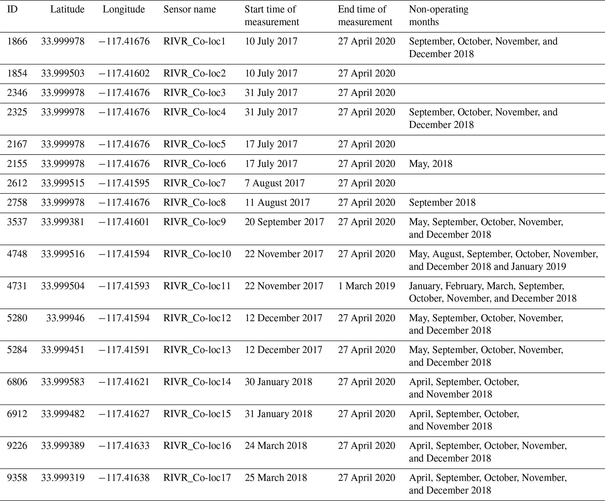
Based on the non-operating months of the PA-II units found, we selected an appropriate period of sample data from January 2018 to December 2019 (24 months). Among the 14 identified PA-II units, we chose several that had more than 23 months of valid measurement data during the period selected for study. The selected units are RIVR_Co-loc2, 3, 5, 6, 7, and 8, which we call PA-II 2, 3, 5, 6, 7, and 8, respectively.

Before using PM_2.5 data from the PA-II units, we checked the units' data quality. We calculated the correlation among the selected PA-II units considering both PMS 5003 sensors for each PA-II unit for the correlation analysis. Since these PA-II units are closely located, PM_2.5 data should be highly correlated. Figure 1 shows the correlation results for all PMS 5003 sensors included in the PA-II units. The numbers on each axis represent the number of the selected PA-II units. Boxes to the left and right of each number indicate PMS sensors A and B for its corresponding PA-II unit, respectively. The PMS sensor A of PA-II unit 2, PMS sensors A and B of PA-II unit 5, and PMS sensor A of PA-II unit 6 all have a poor correlation with other PMS sensors. In addition, sensor A of PA-II unit 3 has slightly poor correlation with other sensors. Based on these results, we selected PA-II units 7 and 8.

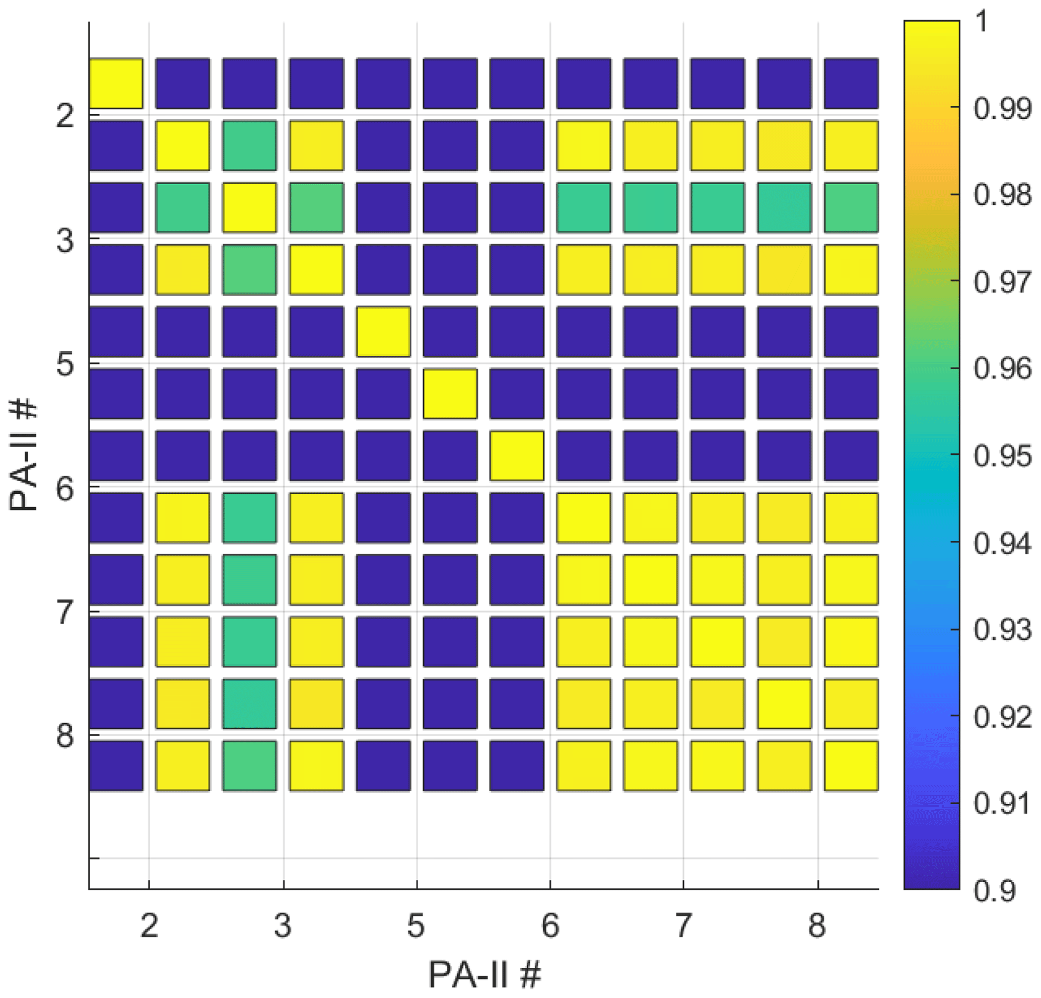
Figure 1 Correlation among all PMS 5003 sensors of the selected units PA-II 2, 3, 5, 6, 7, and 8. The left and right of each number on the x axis represent PMS A and B sensors for its corresponding PA-II unit, respectively.

2.1.4 Data preprocessing of PA-II units

The PA-II units selected for study are long-term installations; i.e., they have been in operation for more than 2 years. Therefore, PA-II units may have abnormal data due to failure and aging drift, so data quality control is required before calibrating the PA-II units. The quality control (QC) measure has been shown to be important for developing correction models of PA-II units (Barkjohn et al., 2021). Barkjohn et al. (2021) performed a QC measure by obtaining daily PM_2.5 measurement data, but we applied the QC measure to obtain hourly PM_2.5 measurement data. The QC measure has the following three steps: (i) data from both channels A and B were removed when either channel A or B had a missing value, (ii) data with abnormal temperature or relative humidity values were removed, and (iii) data from channels A and B were compared. In the first step, when we calculate 1 h averages of PM_2.5 measurements generated with 2 min (or 80 s) intervals, we remove the 1 h average if the number of PM_2.5 measurements is less than 27 (or 40). We considered two different measurement intervals for a PA-II unit because its old interval had been 80 s until 30 May 2019. Its current interval is 2 min. After calculating 1 h average data, we removed all data points for the 1 h interval, where either sensor A or B had a missing value. The second step deals with temperature and RH data. PA-II units occasionally report extremely high or low values of temperature and relative humidity that are inaccurate. Therefore, we removed the data points whose corresponding time interval contained unrealistic measurements of temperature or relative humidity. In this study, the acceptable ranges of temperature and RH are (0 °F, 200 °F) and (0 %, 100 %), respectively. Once the unacceptable data points were removed, we calculated the 1 h average for temperature and RH. The last step was to compare results for sensors A and B in a PA unit to check data consistency. To do this, we used the symmetric percentage error (SPE) as follows:

$$\begin{array}{}\text{(1)}& \text{SPE}={\displaystyle \frac{\mathrm{2}\left(\left|{\text{PM}}_{\mathrm{2.5}}^{\mathrm{A}}\right|-\left|{\text{PM}}_{\mathrm{2.5}}^{\mathrm{B}}\right|\right)}{|{\text{PM}}_{\mathrm{2.5}}^{\mathrm{A}}+{\text{PM}}_{\mathrm{2.5}}^{\mathrm{B}}|}},\end{array}$$

where PM${}_{\mathrm{2.5}}^{\mathrm{A}}$ and PM${}_{\mathrm{2.5}}^{\mathrm{B}}$ are hourly averaged PM_2.5 concentrations from sensors A and B in the same PA-II unit, respectively. We removed the relevant data points with SPE larger than 0.61, which is 2 standard deviations. This value of SPE threshold has been used for 24 h average PM_2.5 concentrations (Barkjohn et al., 2021), but we use it here for 1 h averaged PM_2.5 concentrations. The number of data points processed for each pre-processing step in PA-II 7 is summarized in Table S2.

The period of valid measurement data collected from the PA-II units we selected is 24 months, such as from January 2018 to December 2019. The measurement data in the years 2018 and 2019 from the 2-year dataset were used for training and testing for our calibration models, respectively. The reason why we split the 2-year dataset at a 1:1 ratio is that PM_2.5, as well as the other environmental parameters, such as temperature and relative humidity, which we considered for calibration models, have a seasonal pattern. Also, we used whole-year dataset for training to learn the relationship between PA-II and regulatory measurement over seasonality and thus enhance the performance of the calibration models over all four seasons.

2.2 Instrument intercomparisons

The monitoring site we considered has an FRM instrument and a BAM-1020 instrument with the parameter of 88502. These instruments produce daily and hourly PM_2.5 measurement data, respectively. Since we measure the PA-II units at intervals much shorter than a full day, it is much more reasonable to compare the PM_2.5 measurement of PA-II units with that of a BAM-1020 instrument with a shorter measurement interval rather than that of an FRM instrument for evaluating the accurate calibration performance of PA-II units. However, we face the limitation that a BAM-1020 instrument can be classified as a non-FEM-compliant device. Therefore, our approach for analyzing PA-II units to appropriately resolve these issues is as follows: we compared the BAM-1020 instrument's readings with daily PM_2.5 concentrations collected from an FRM instrument to ensure that the BAM-1020 provides an acceptable level of performance as an FRM instrument, which is enough to assess the calibration performance of PA-II units. According to this affirmative observation, the BAM-1020 instrument can be used to evaluate the calibration performance of low-cost PM_2.5 sensors by comparing its readings with hourly PM_2.5 measurement data of PA-II units.

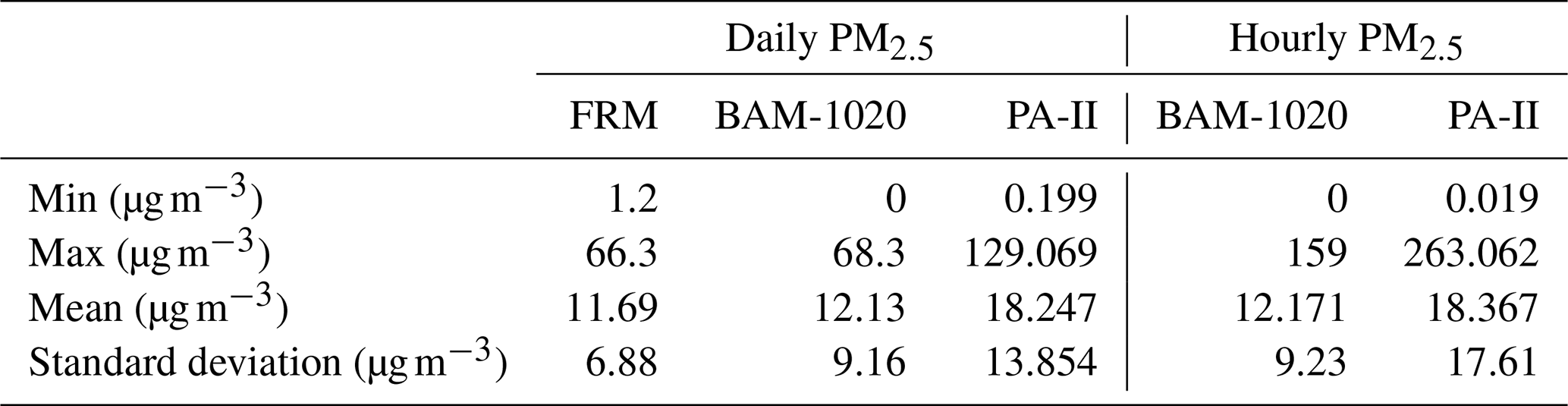
We compared daily and hourly PM_2.5 measurement data obtained from FRM and BAM-1020 instruments and a PA-II 7 unit. Table 3 shows summary statistics of daily and hourly PM_2.5 measurement data from FRM and BAM instruments and PA-II 7³. These data suggest that a BAM-1020 instrument using non-FEM methods compares well to the statistics achieved with the FRM method. However, the measurements are not enough to evaluate how similar the performance of the BAM-1020 is to that of the FRM instrument. Hence, this study compared the performance of two instruments using a linear fitting scheme. Figure 2 shows the calibration performance using linear regression. The R², slope, and intercept are 0.896, 0.923, and 0.741, respectively. Also, the value of RMSE is 2.211  µg m⁻³. The BAM-1020 is close to an FEM instrument with the parameter of 88101. In order for the BAM-1020 to attain the 88101 code in terms of performance, the following conditions must be satisfied: R² is larger than 0.9, the slope is larger than 0.9 and less than 1.1, and the absolute value of the intercept is less than 2.0. Slope and intercept are satisfied with the requirement, while R² does not meet the condition very slightly. Nonetheless, the BAM-1020 instrument provides an acceptable level of performance to evaluate the calibration performance of PA-II units on an hourly basis.

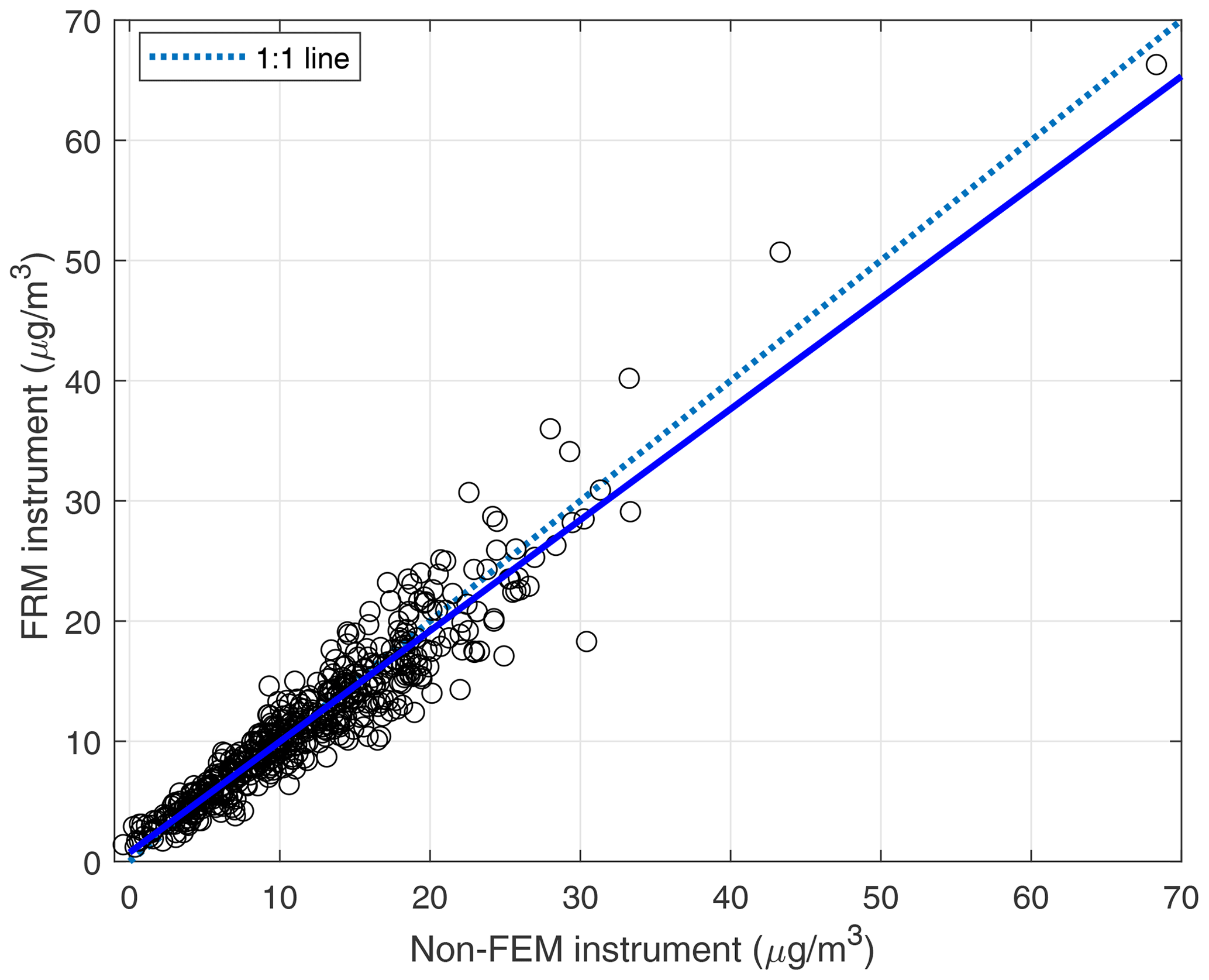
Figure 2 Scatter plot for daily PM_2.5 comparison of BAM-1020 (non-FEM) instrument with the FRM instrument.

Compared to the FRM and BAM-1020 instruments, the PA-II 7 unit overestimates the maximum daily PM_2.5 concentrations. Additionally, the mean daily PM_2.5 concentration from the PA-II 7 unit was higher than that of the FRM and BAM-1020 instruments. These results show that the PA-II unit has a good correlation (r) with the FRM instrument for the 2-year period of interest since its value is very close to 1. However, a comparison of metrics from the FRM instrument and the PA-II 7 unit did not correlate as favorably.

Next, we compared the PA-II unit's hourly PM_2.5 data with those of the BAM-1020 instrument over the course of the same 2-year period. We did not consider the FRM instrument for exploring hourly PM_2.5 measurement data since it only produces daily concentrations. The PA-II unit's maximum hourly PM_2.5 measurement was almost twice that of the BAM-1020. In other words, the PA-II unit overestimates hourly PM_2.5 concentrations. Figure 3 shows the comparison of PM_2.5 measurement data obtained from the BAM-1020 and the selected PA-II 7 unit, as well as temperature and relative humidity measured from the selected PA-II 7 unit during the winter season (from December 2018 to February 2019). The PA-II 7 unit showed a similar trend of PM_2.5 concentration measurements to that of the BAM-1020 instrument, but it generally overestimated hourly PM_2.5 concentrations more often than the BAM-1020.

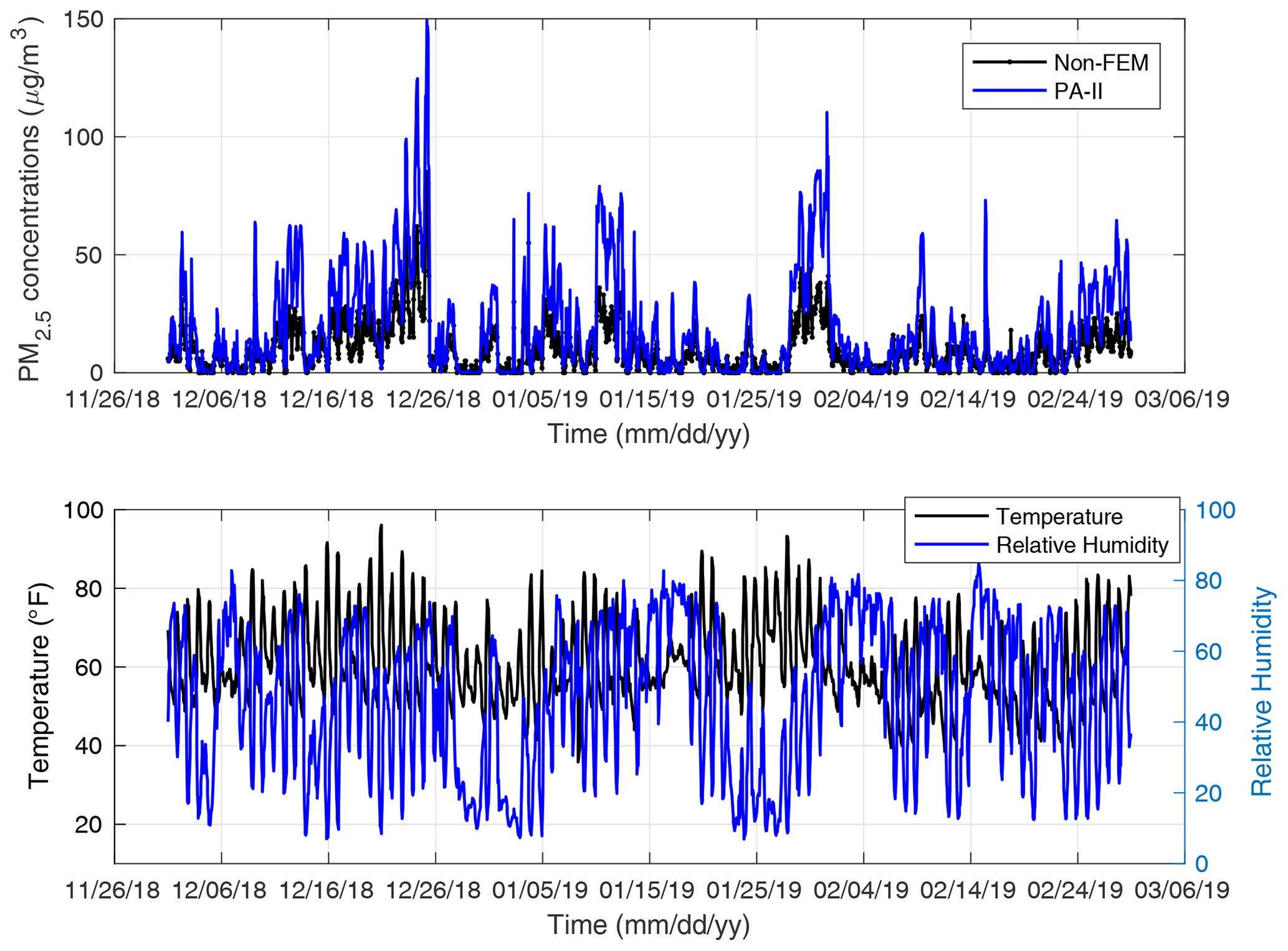
Figure 3 Hourly PM_2.5 concentrations measured by BAM-1020 (non-FEM) and PA-II 7 and hourly temperature and relative humidity measured by PA-II 7 from December 2018 to February 2019.

In addition, we compared the hourly PM_2.5 concentrations of the PA-II unit with those of the BAM-1020 instrument in terms of root-mean-square error (RMSE), mean-square error (MSE), mean absolute error (MAE), and correlation (r). The results are as follows: RMSE of 6.194 µg m⁻³, MSE of 38.369 µg m⁻³, MAE of 7.919 µg m⁻³, and r of 0.876. The PA-II unit had a good correlation with the BAM-1020 instrument based on r. However, other metrics, such as RMSE, MSE, and MAE, did not correlate well.

2.3 Feature selection for calibration models

Temperature and relative humidity have been identified in previous studies as key factors for effective calibration. In particular, relative humidity has been shown to affect low-cost PM sensors under high-relative-humidity conditions. Furthermore, few papers have considered NO₂ in calibration models (Hua et al., 2021) because NO₂, which is known to be a precursor to the formation of PM_2.5 through chemical reactions in the atmosphere, may indirectly affect PM_2.5 concentrations. Therefore, we investigated the suitability of temperature, relative humidity, and NO₂ for the calibration of the PA-II 7 unit.

To identify the independent variables relevant for calibration, we conducted a correlation analysis involving PM_2.5 measurements from BAM-1020 and PA-II 7 unit readings, as well as temperature and relative humidity data, spanning a 2-year period. The results are illustrated in Fig. S2. The highest correlation was observed between PM_2.5 from BAM-1020 and the PA-II 7 unit, followed by NO₂ measurements. Subsequently, relative humidity and temperature exhibited the next level of correlation. As a result, we have identified temperature, relative humidity, and NO₂ as the selected candidate features.

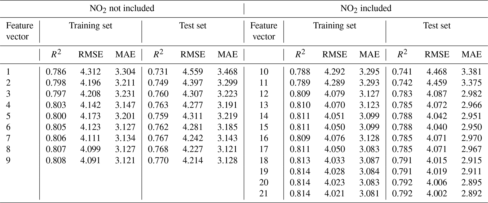
To explore the potential for enhancing the calibration performance of low-cost PM sensors using temperature, relative humidity, and NO₂ as features, we conducted linear fitting. Before considering temperature, relative humidity, and NO₂, we evaluate the monthly performance based on hourly PM_2.5 data from the PA-II 7 unit compared to the BAM-1020 instrument. Table 2 shows the values of the R², RMSE, and MAE of hourly PM_2.5 measurement data from the PA-II 7 unit compared to those of the BAM-1020 instrument and the corresponding slope and intercept of each optimal linear fitting. During the months of November, December, and January, the PA-II unit is shown to have a high correlation – R² of 0.813 to 0.936 – with the BAM-1020 instrument. This result is supported by the field evaluation of PA-II units conducted by the Air Quality Sensor Performance Evaluation Center (AQ-SPEC) during the period of December 2016–January 2017, which showed the value of R² as being 0.868 to 0.921 when the PA-II units were compared with the FEM. Sayahi et al. (2019) showed that PMS sensors have a high correlation with tapered element oscillating microbalance (TEOM) instruments during the winter season by providing R² of 0.866 to 0.892. That is, the hourly PM_2.5 measurement data from PA-II units seem to be highly correlated with those of FEM instruments during the months of November, December, and January, which implies that the PM_2.5 measurement performance of PA-II is reliable, especially during winter seasons. These months have different slopes and intercepts; for example, January 2018 has a slope of 0.502 and an intercept of 3.898, while January 2019 has a slope and intercept of 0.397 and 1.961, respectively.

Table 2 R², RMSE, and MAE of the PA-II unit against the BAM-1020 based on the hourly PM_2.5 measurement data for each month.

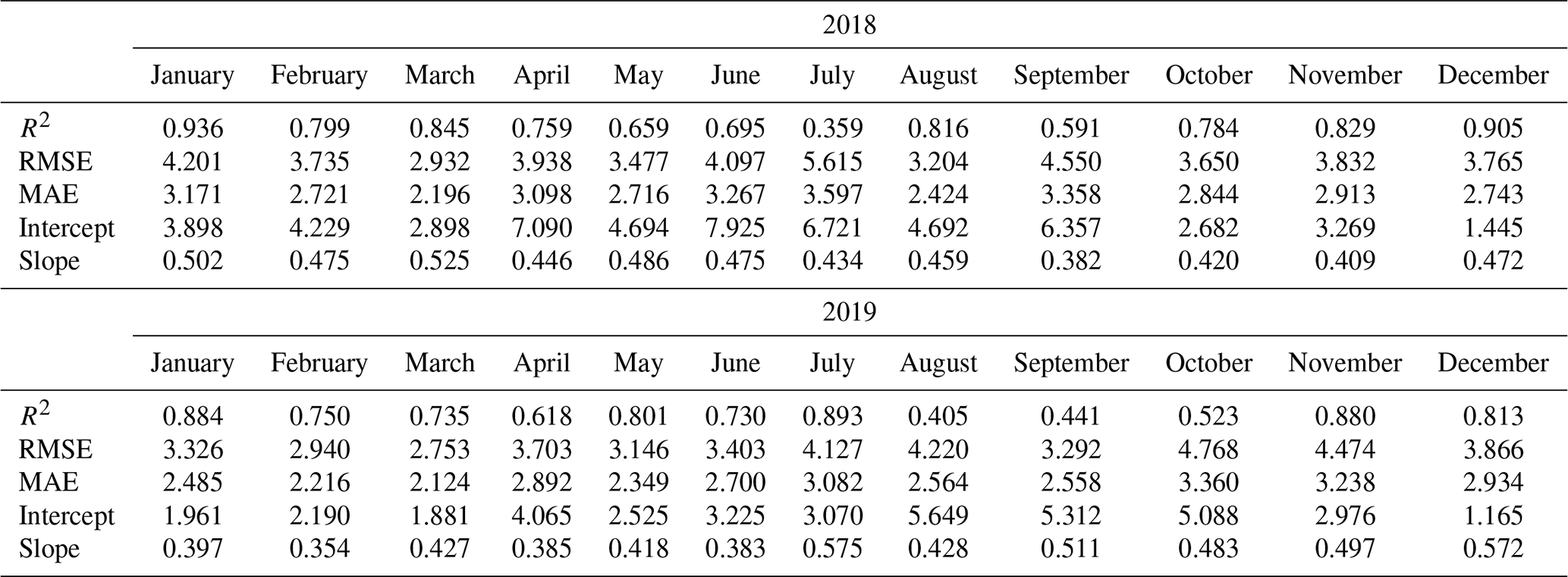
Table 3 Summary statistics of daily and hourly PM_2.5 measured from an FRM, BAM-1020, and PA-II 7 unit.

On the other hand, the PA-II 7 unit has a correlation lower than 0.6 for the months of July and September 2018, as well as of August, September, and October 2019. These months, except September 2019, have larger RMSE values compared to other months over the 2-year period, which need to be calibrated.

For multiple features, such as temperature, relative humidity, and NO₂, we used an MLR approach for regression analysis of PA-II units compared to the BAM-1020 instrument. A per-month analysis was conducted based on hourly PM_2.5 measurements from the PA-II 7 unit under several feature vectors, such as (PM_2.5), (PM_2.5, T), (PM_2.5, RH), (PM_2.5, NO₂), (PM_2.5, T, RH), and (PM_2.5, T, NO₂), where T and RH represent temperature and relative humidity, respectively. For notational simplicity, we defined the above feature vectors of (PM_2.5), (PM_2.5, T), (PM_2.5, RH), (PM_2.5, NO₂), (PM_2.5, T, RH), and (PM_2.5, T, NO₂) as 1, 2, 3, 4, 5, and 6, respectively. Figure 4 shows the R² and RMSE results of multiple linear regression for selected months with the above varying feature vectors. We considered feature vector 1 as a baseline for comparison among other feature vectors. On January 2018, feature vector 5, referring to temperature and relative humidity, had little effect on the regression performance of R² and RMSE. The amount of R² increase by feature vector 5 from the baseline was around 0.001, and the amount of RMSE decrease was 0.038 µg m⁻³. In the case of feature vector 6, including NO₂ instead of RH, R² increased from the baseline by 0.015, while RMSE was improved by 0.518 µg m⁻³. Similarly, for April 2018, R² (or RMSE) for feature vector 5 increased (or decreased) by 0.01 (or 0.072 µg m⁻³) compared to its baseline. R² and RMSE for feature vector 6 increased by 0.05 and decreased by 0.52 µg m⁻³ from the baseline, respectively. For regressions in August and September 2019, an increase in R² was larger than 0.17 when feature vector 6 was considered, but it was less than 0.07 when feature vector 5 was considered. These remarkable results suggest that NO₂ is generally a key factor that can improve the performance of PA-II units over a year, even though the enhancement by NO₂ does not meet the values of 0.7 of R² and 3.5 µg m⁻³ of RMSE during certain months, such as July 2018, August 2019, and October 2019.

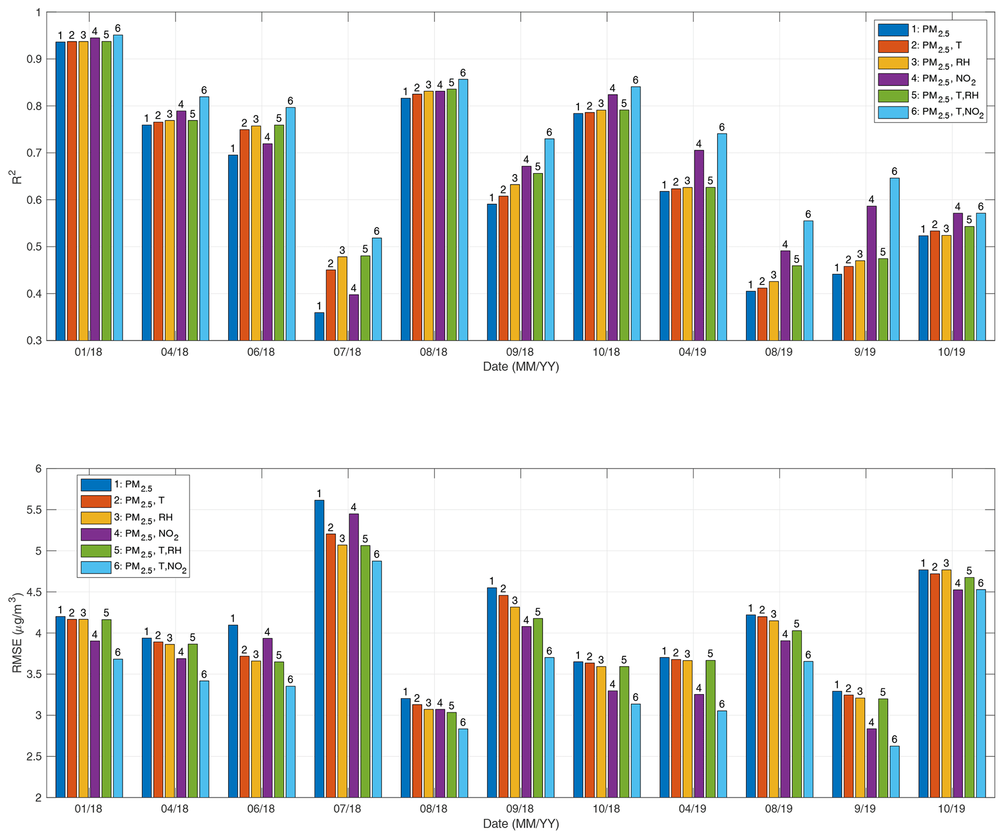
Figure 4 R² and RMSE using MLR method for the PA-II unit with the BAM-1020 for the selected months based on the following feature vectors: 1 – (PM_2.5), 2 – (PM_2.5, T), 3 – (PM_2.5, RH), 4 – (PM_2.5, NO₂), 5 – (PM_2.5, T, RH), and 6 – (PM_2.5, T, NO₂).

2.4 Calibration methods

A per-month analysis with a combination of features, including T, RH, and NO₂, showed an effect on calibration for the PA-II unit. However, it is challenging to use the per-month linear fitting result to calibrate PA-II units because each month has a different slope and intercept defined for the linear fitting. Moreover, their values exhibit a change over the years. For example, notably, the linear fitting result in April 2018 exhibited a higher RMSE than the fitting result in April 2019. On the contrary, the calibration performance in August 2018 was worse than that in August 2019.

We used a machine learning approach to develop a calibration model, employing two machine learning algorithms, such as multiple linear regression (MLR) and random forest (RF). For both calibration methods, we considered various combinations of features, including PM_2.5 measured from a PA-II unit, temperature, relative humidity, NO₂, and their multiplicative interaction terms.

2.4.1 Multiple linear regression (MLR)

An MLR method can be expressed as follows:

$$\begin{array}{}\text{(2)}& \widehat{y}={\mathit{\beta }}_{\mathrm{0}}+{\mathit{\beta }}_{\mathrm{1}}{x}_{\mathrm{1}}+\mathrm{\dots }+{\mathit{\beta }}_n{x}_n,\end{array}$$

where $\widehat{y}$ represents a response; n is the number of predictor variables; β_i values for $i=\mathrm{0},\mathrm{1},\mathrm{\dots },n$ are regression coefficients; and x_i values for $i=\mathrm{1},\mathrm{2},\mathrm{\dots },n$ represent predictor variables (called features). Using a linear equation with multiple variables, we investigated the relationship between features and a response.

All features in an MLR method should be independent. However, many studies have considered PM_2.5, temperature, and RH, which are not independent (Magi et al., 2019; Malings et al., 2020). Some studies have introduced multiplicative interaction terms (i.e., PM_2.5× RH) to exploit interdependence between features (Barkjohn et al., 2021). We also consider multiplicative interaction terms in this study.

We use PM_2.5 concentrations obtained from a reference monitor as the response. As predictor variables, we consider multiple features, such as PM_2.5 measurement data from a PA-II unit, temperature, relative humidity, NO₂, and their multiplicative interaction terms (i.e., PM_2.5× RH, T× RH, PM_2.5× RH ×T).

2.4.2 Random forest (RF)

An RF is an ensemble of K regression trees. Each regression tree is trained with a bootstrap sample of an original training dataset. The output of an RF is the aggregation of regression trees, i.e., averaging estimates over all trees. Each regression tree is grown by selecting random m features among M input features at each possible split. The best cut is calculated for the randomly chosen features. Optimal cuts can be achieved using the classification and regression tree split criterion (CART), which compares the variance of the uncut node and one of all possible cuts along m directions. Every tree is fully grown with these splits (Breiman, 2001).

2.5 Performance evaluation metrics

In this study, we examined the root mean square error (RMSE), mean squared error (MSE), mean absolute error (MAE), and Pearson correlation coefficient r between daily PM_2.5 data from the FRM instrument and from the PA-II units. In the cases of the RMSE, MSE, and MAE, the lower its value is, the better the performance or the lower the difference in measurement data between the FRM instrument and the PA-II units. The Pearson correlation coefficient is a metric measuring a linear correlation between two variables. It is a number between −1 and 1 that measures the strength and direction of their relationship. As the coefficient approaches an absolute value of 1, the values of measurement data fromthe FRM instrument and the PA-II units become more similar. These performance metrics are expressed as follows:

$$\begin{array}{}\text{(3)}& {\displaystyle }\text{RMSE}=\sqrt{{\displaystyle \frac{\mathrm{1}}{n}}\sum _{i=\mathrm{1}}^n(x_i-y_i{)}^{\mathrm{2}}},\text{(4)}& {\displaystyle }\text{MSE}={\displaystyle \frac{\mathrm{1}}{n}}\sum _{i=\mathrm{1}}^n(x_i-y_i{)}^{\mathrm{2}},\text{(5)}& {\displaystyle }\text{MAE}={\displaystyle \frac{\mathrm{1}}{n}}\sum _{i=\mathrm{1}}^n|x_i-y_i|,\end{array}$$

where x_i represents 1 h averaged (24 h period) sensor PM_2.5 concentrations for the ith hour (day) (µg m⁻³), y_i represents 1 h averaged (24 h period) FRM or BAM-1020 PM_2.5 concentrations for the ith hour (day) (µg m⁻³), and n is the number of data points.

3 Results and discussions

3.1 Calibration performance

The 2-year dataset was divided into training and test sets at a 1:1 ratio, meaning the measurement data in the years 2018 and 2019 were used for training and testing, respectively. We used the training set to learn calibration models based on MLR and RF, and then we used the test set to evaluate the calibration performance in terms of RMSE, MAE, and R². A calibration performance for the PA-II 7 unit using MLR and RF methods was compared with several features, including temperature, relative humidity, and NO₂, as well as their multiplicative terms.

3.1.1 MLR-based calibration model

Recently, calibration methods have employed multiplicative interaction terms, such as PM_2.5× RH and T× RH. In our MLR models, we considered both additive and multiplicative interaction terms. The additive terms in our models include raw PurpleAir PM_2.5, T, RH, and NO₂. We considered multiplicative interaction terms that involve fewer than four additive terms when NO₂ was not included (i.e., we consider PM${}_{\mathrm{2.5}}\times T\times$ RH) and fewer than three additive terms when NO₂ was included. There are 95 combinations of features. Out of 95 combinations tested, only 52 combinations had a p value of less than 0.05. Of those, we select 21 combinations, among 52 combinations, by increasing the number of additive terms and the number of multiplicative interaction terms and identifying the combinations with the lowest RMSE among the same numbers of additive terms and multiplicative interaction terms. The selected combinations were shown in Table 4.

Table 4 A list of selected feature vectors in MLR methods.

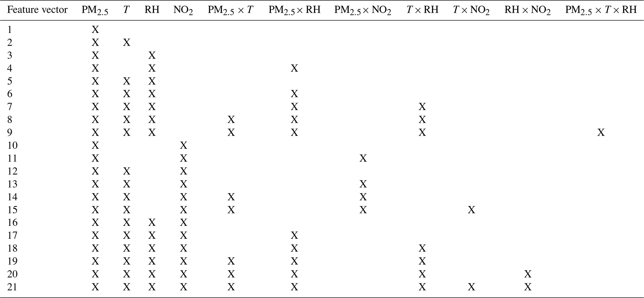
The calibration results of the PA-II 7 unit for test datasets using the MLR method with 21 selected combinations are presented in Table 5. Multicollinearity is a known issue with MLR models as it can cause instability. One common method to diagnose this issue is to use the variance inflation factor (VIF) test for multicollinearity (Mansfield and Helms, 1982). Out of the 21 combinations tested, most VIF values were less than 5, indicating the absence of collinearity issues.

Table 5 Calibration results (R², RMSE (µg m⁻³), and MAE (µg m⁻³)) of hourly PM_2.5 concentrations using MLR for the PA-II 7 unit based on the selected combinations.

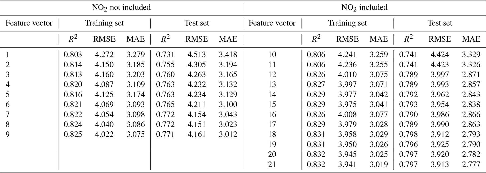
When a single additive term, such as T or RH, was applied, the RMSE values for two combinations, no. 2 and no. 3, improved by more than 0.208 µg m⁻³ compared to that considering only PM_2.5. The inclusion of an additive RH term in an MLR yielded a lower error than an additive T term did since both RMSE and MAE for combination no. 3 were less than those for combination no. 2. The MLR model with PM_2.5, the single additive term with RH, and its multiplicative interaction term with PM_2.5 yielded similar RMSE and MAE values to the MLR model using PM_2.5 and two meteorological variables, such as T and RH, as demonstrated by the results of combinations no. 4 and no. 5. When we considered two meteorological variables and incorporated four multiplicative interaction terms, such as PM_2.5×T, PM_2.5× RH, and T× RH, the MLR model resulted in the lowest error, with an RMSE of 4.151 µg m⁻³ and an MAE of 3.023 µg m⁻³, compared to all combinations generated from PM_2.5, T, RH, and their multiplicative terms.

The MLR model of combination no. 10 with PM_2.5 and NO₂ had an RMSE of 4.424 µg m⁻³, which was lower than that of the MLR model with only PM_2.5, whose RMSE was 4.513 µg m⁻³, but larger than that of combination no. 2 with a single environmental variable and an RMSE of 4.305 µg m⁻³. This implies that the addition of a single multiplicative term in that model has no performance enhancement. However, when the additive term T is incorporated into an MLR model with PM_2.5 and NO₂, an RMSE of 3.997 µg m⁻³ can be achieved, which is lower than the values of all combination cases not including NO₂, i.e., combinations no. 1 to no. 9. Coefficients of PM_2.5, T, and NO₂ in the MLR model, including T and NO₂, were around 0.446, 0.110, and 0.112, respectively. The temperature had more impact on error than relative humidity when considering NO₂. Considering both temperature and relative humidity together with NO₂ may cause a non-zero correlation of relative humidity with other factors due to a p value of 0.083. When some multiplicative terms were additionally integrated into T, RH, and NO₂, the MLR calibration models passed a p-value test. The model based on combination no. 18 with four additive terms, i.e., PM_2.5, T, RH, and NO₂, and multiplicative interaction terms, including PM_2.5× RH and T× RH, achieved the lowest RMSE of 3.912 µg m⁻³. Considering multiplicative terms with T and RH had little effect on calibration performance, as shown in the results of combination nos. 15, 19, and 20. From these results, we conclude that considering NO₂ together with meteorological variables and their multiplicative terms or a single variable, such as temperature, can improve the calibration performance of PA-II units.

3.1.2 RF-based calibration model

This study validated the performance of RF-based calibration for PA-II units with 95 combinations of predictor variables mentioned in the previous subsection. An RF was implemented using the scikit-learn package in Python. An RF has several hyperparameters, such as n_estimators, max_depth, min_samples_leaf, and max_features, that need to be set for the best performance over each combination of features. For this study, the hyperparameters were tuned with a random search method by 5-fold cross-validation based on the training set. For a random search, the number of trees (n_estimators) was set to 10, 20, 50, 100, 200, and 400. The range of max_depth was set to 2, 4, 6, 8, 10, 16, and none. The range of min_samples_leaf was set to 1, 2, 3, 4, and 5. The range of min_samples_split was set to 2, 3, 5, 7, and 10. The range of max_features was set to none.

We selected 22 combinations according to the above-mentioned method. The selected combinations were listed in Table 6. Table 7 summarizes calibration results, including R², RMSE, and MAE values of test sets for PA-II units using the RF method with the selected combinations of features.

Table 6 A list of selected feature vectors in RF methods.

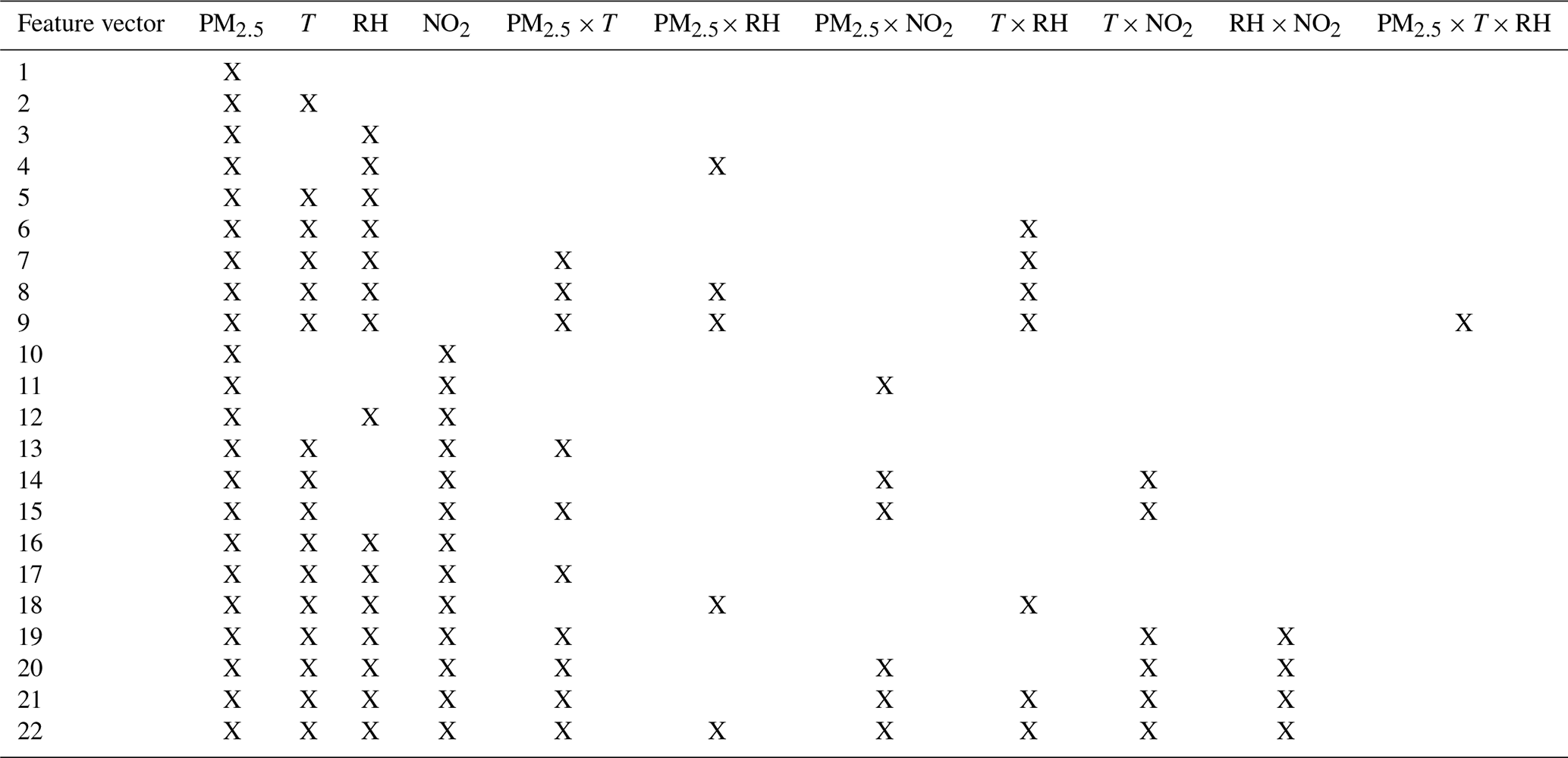
Table 7 Calibration results (R², RMSE (µg m⁻³), and MAE (µg m⁻³)) of hourly PM_2.5 concentrations using RF for the PA-II 7 unit based on the selected combinations.

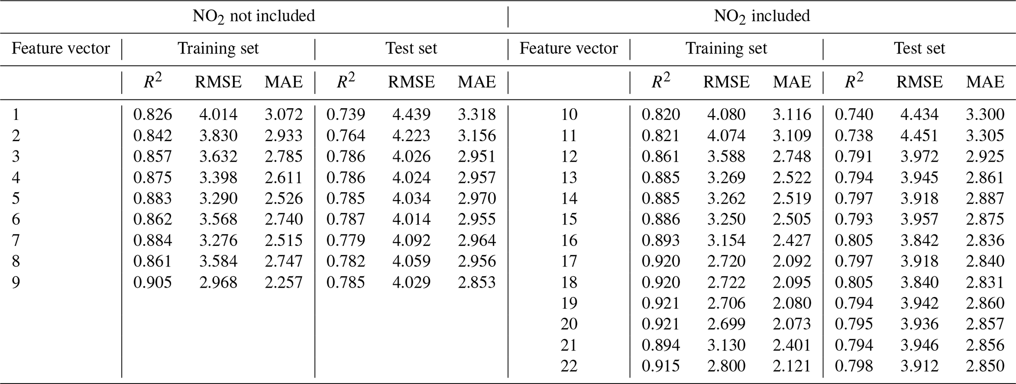
Like the MLR method, the RF method showed better performance in the training set than in the test set. Some combinations had RMSE differences larger than 0.6 µg m⁻³ between training and test sets, while others had differences smaller than 0.4 µg m⁻³. We note that some combinations with multiplicative terms showed significant RMSE differences between two datasets, which might have occurred because of overfitting of the training dataset. Nonetheless, the RF models with the other combinations had lower RMSE values than the model using only PM_2.5. Considering a single environmental variable together with PM_2.5 improved the calibration performance in terms of values of RMSE and MAE compared to the RF model with only PM_2.5. Specifically, RH had a more significant impact on the performance enhancement of the RF calibration model than T, as seen in the results of combination nos. 2 and 3. Including the additional multiplicative term of PM_2.5× RH had an insignificant effect on RMSE compared to the RF model with PM_2.5 and RH. Both meteorological variables together, i.e., combination no. 5, yielded lower RMSE values in the training set compared to in the RF model with PM_2.5 and RH, i.e., combination no. 3, but similar RMSE values in the test set. In contrast to MLR models, more than one multiplicative term, i.e., combination nos. 6 to 9, bring about insignificant differences in RMSE compared to considering a single meteorological variable. When we analyze calibration methods without NO₂, the RF model with PM_2.5, T, and RH improved RMSE by 0.117 µg m⁻³ compared to the best MLR model.

Utilizing NO₂ in RF models had different effects on calibration performance, depending on the combinations of predictor variables. The RF model of combination no. 10 with the additional NO₂ term resulted in an RMSE of 4.434 µg m⁻³, which showed little improvement compared to combination no. 1 with only PM_2.5 and an RMSE of 4.439 µg m⁻³. The RF model with PM_2.5 and NO₂ had a larger RMSE than the MLR model with the same features, but the difference was not significant; it did not show enough performance improvement to warrant adding the multiplicative term of PM_2.5× NO₂ from combination no. 10. Adding a single or two meteorological variables to RF models of combination nos. 12 and 16 lead to remarkable performance enhancement over combination no. 10 with RH, with RMSE decreasing by 0.462 µg m⁻³. Furthermore, RMSE dropped by an additional 0.130 µg m⁻³ when T was added as an additional feature. The combinations consisting of one or more multiplicative interaction terms resulted in either an insignificant improvement or a slight decline in the performance in terms of RMSE and MAE when compared with combination no. 16, consisting of PM_2.5, T, RH, and NO₂. In other words, there is no need to consider multiplicative interaction terms when using the RF model because there is no outstanding performance improvement.

As with the MLR method, it was shown that including NO₂ as a consideration in RF methods can improve calibration performance. Moreover, by integrating two additional variables, such as T and RH, even better calibration performance can be achieved.

The RF method was shown to have a better performance than the MLR method when NO₂ was not considered. From the viewpoint of RMSE, the best performances from MLR and RF methods were 4.151 and 4.014 µg m⁻³, respectively. However, when we consider NO₂, the best MLR model is not significantly different from the best RF model. For instance, the RMSE values from the best MLR and RF models were 3.912 and 3.840 µg m⁻³, respectively. Their corresponding R² values differ slightly since their gap is only 0.008. Nonetheless, the MAE of 2.777 µg m⁻³ achieved from the best MLR is lower than that achieved by the best RF, which is 2.831 µg m⁻³. From these results, we conclude that better calibration can be obtained by considering NO₂ additionally. Furthermore, when NO₂ is considered, the MLR model can enhance calibration performance without the need for an RF model.

3.2 Effect of distant NO₂ on calibration performance

In the previous subsections, it was demonstrated that including NO₂ as a consideration can effectively improve the calibration performance of PA-II units. However, it is not always feasible to have an NO₂ instrument with high accuracy collocated with a low-cost PM sensor. Instead, an alternative approach is to collocate a low-cost NO₂ sensor with a PA-II unit, but this approach is hindered by the unreliability of NO₂ sensors. To address this issue, we investigated the usefulness of using data from distant NO₂ instruments installed with PA-II units for the calibration algorithm.

We selected two monitoring sites that measure NO₂ near the Rubidoux site. Two monitoring sites identified were 06-065-8005 and 06-071-0027. The distances between the two monitoring sites and the Rubidoux site are 7.05 and 18.87 km, respectively. The correlations of NO₂ measurements obtained from the Rubidoux site with those of 06-065-8005 and 06-071-0027 were 0.895 and 0.621, respectively. The site 06-065-8005 had NO₂ measurements that were much more highly correlated with the Rubidoux site compared with those from the site 06-071-0027. This result can occur when the distance from the Rubidoux site to the site 06-065-8005 is shorter than it is to the site 06-071-0027.

To evaluate the usefulness of distant NO₂ measurements in the calibration of a low-cost PM sensor, we used NO₂ data measured from monitoring sites near the PA-II 7 unit as a test dataset rather than data from the collocated Rubidoux site. When we trained calibration models with the measurements from the PA-II 7 unit over 2018, we used highly accurate NO₂ concentrations measured by FEM instruments at the Rubidoux site. Subsequently, to verify the trained calibration models, we utilized a separate test dataset featuring distant NO₂ measurements taken by FEM instruments at sites 06-065-8005 and 06-071-0027. We considered this scenario to evaluate our proposed calibration models, previously trained with collocated NO₂ concentrations and distant NO₂ concentrations, when collocated NO₂ measurements cannot be collected.

Table 8 shows calibration performance using MLR and RF methods with NO₂ collected from the air quality monitoring sites near the PA-II unit. In the case of MLR methods used with 06-065-8005 data, the difference in RMSE between NO₂ data obtained from a collocated NO₂ instrument, called collocated NO₂, and a distant NO₂ instrument, called distant NO₂, was less than 0.06 µg m⁻³ for every selected combination defined in the previous two subsections for the MLR and RF methods. All MLR models using distant NO₂, except combination nos. 10 and 11, yielded lower errors than all MLR models without NO₂, as shown in Table 5. For example, the worst RMSE of the MLR methods using distant NO₂ data (except combination nos. 10 and 11) was 4.018 µg m⁻³, while the best RMSE without NO₂ was 4.151 µg m⁻³. Like RMSE, other metrics, such as R² and MAE, also showed a calibration performance enhancement for these combinations with distant NO₂.

Table 8 Calibration result (R², RMSE (µg m⁻³), and MAE (µg m⁻³)) of hourly PM_2.5 concentrations using MLR and RF models for the PA-II 7 unit based on the selected combinations with, in addition, distant NO₂.

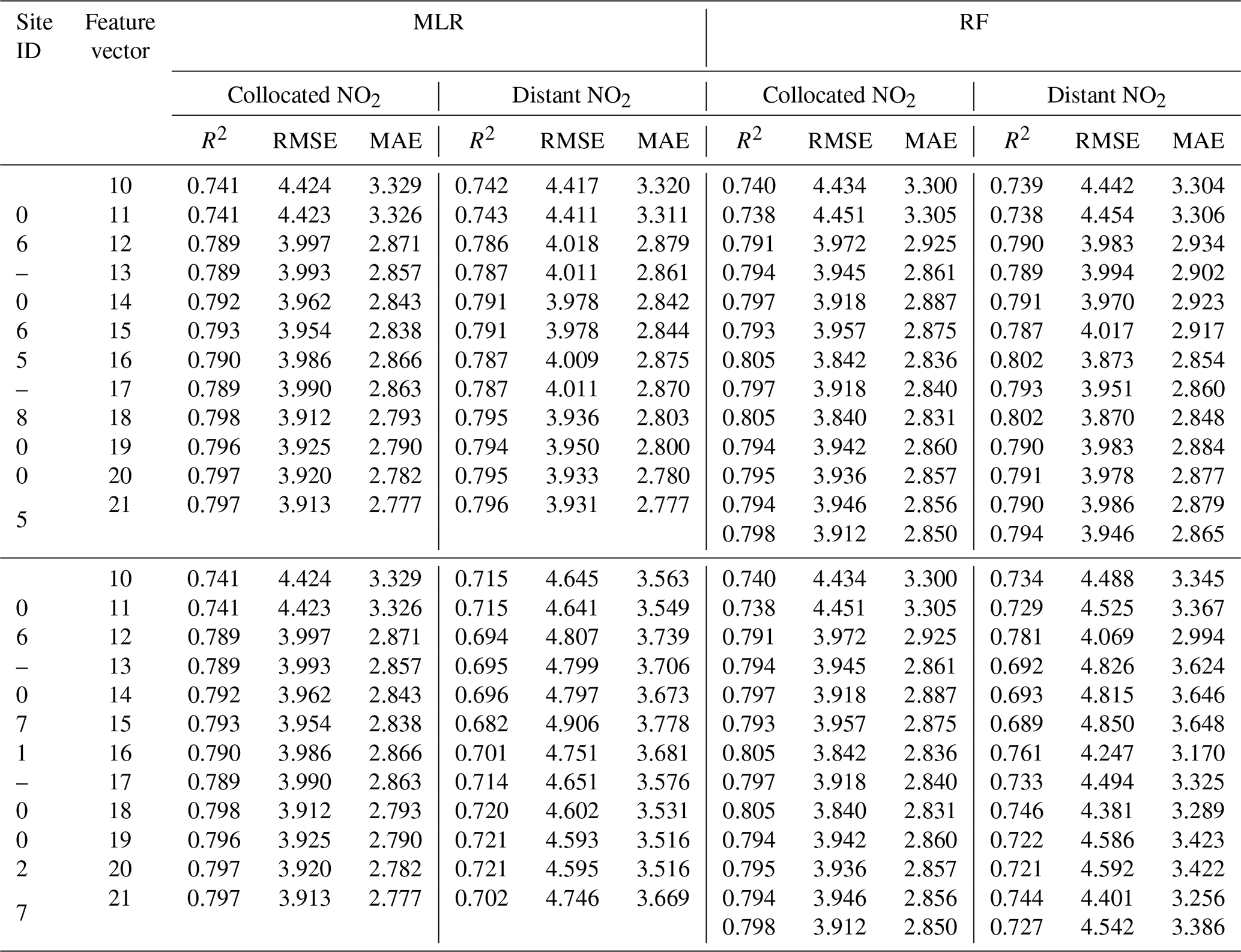
When we used an MLR algorithm with NO₂ data, the result of the calibration performance for the monitoring site 06-071-0027 showed a new aspect compared to that of 06-065-8005. All MLR methods using distant NO₂ data from site 06-071-0027 had a higher RMSE than the MLR algorithm based on data that did not include NO₂ data from the collocated Rubidoux instrument, which had an RMSE of 4.513 µg m⁻³, as shown in Table 5. This result can be explained by comparing the correlation of NO₂ measured from the Rubidoux site with measurements from site 06-065-8005 and from site 06-071-0027. The NO₂ correlation between Rubidoux measurements and site 06-065-8005 was 0.895, while the correlation with site 06-071-0027 was 0.621. These results show that 06-065-8005 data are much more correlated with the Rubidoux site in terms of NO₂.

In the case of RF models, the use of the distant NO₂ data from site 06-065-8005 increased RMSE compared to using collocated NO₂ data but not significantly since the maximum gap of RMSE values for all feature vectors considered was just 0.060 µg m⁻³. Similarly to the MLR method, all RF models referring to distant NO₂ from site 06-065-8005, except combination no. 11, resulted in a better calibration performance than what was seen in combination no. 1 without NO₂, which had an RMSE of 4.439 µg m⁻³, as shown in Table 7. Other metrics, such as R² and MAE, also showed a calibration performance improvement. In the case of RF models using data from site 06-071-0027, calibration performance for each combination was degraded compared to the corresponding combination using collocated NO₂, which had similar results to the MLR model. As we explained previously, the higher the correlation of NO₂ measurements from the Rubidoux site with measurements from sites 06-065-8005 and 06-071-0027, the better the calibration performance of the RF model; that is, all combinations with distant NO₂ from 06-065-8005 provide a lower RMSE than those from 06-071-0027. Moreover, when we consider the fact that 06-065-8005 has a high correlation of NO₂ with the expensive NO₂ instrument collocated with the PA-II 7 unit, the best RMSE for all combinations using the RF model is slightly lower than that based on the MLR method.

In the case of 06-065-8005, RF models using distant NO₂ resulted in lower, but insignificant, RMSE values compared to MLR models using distant NO₂. From these results, we draw the conclusion that the use of NO₂ collected from distant instruments with a high correlation with a collocated NO₂ site of PA-II units can improve the PA-II unit's calibration performance. Furthermore, both MLR and RF models can be good calibration models when distant NO₂ is considered. This is different from the conclusion that calibration performance of RF models is better than MLR models (Zimmerman et al., 2018).

3.3 Applicability of other PA-II units

We evaluated PA-II 8's calibration performance in the following three cases:

1. Case 1. The calibration model is learned with the measurements collected from the PA-II 8 in 2018, and the calibration performance for the trained model is evaluated using data measured from the PA-II 8 in 2019.

2. Case 2. This is similar to Case 1, except that the calibration model is trained with the data measured from the PA-II 7 in 2018.

3. Case 3. The measurement data from the PA-II 8 with collocated NO₂ concentration in 2018 are used as a training dataset, while the data collected from the PA-II 8 with either collocated NO₂ or distant NO₂ concentration in 2019 are used as a test dataset.

In Case 1, we evaluated the calibration model's performance with a test dataset consisting of measurement data from the PA-II 8 in 2019. The calibration model is trained with data collected from the same PA-II 8 in 2018. Table 9 shows the calibration results of the PA-II 8 using an MLR method under two different cases: with and without NO₂. We selected the same feature vectors as defined in Table 4. We observed that NO₂ can enhance calibration performance because all MLR models using NO₂, except combination nos. 10 and 11, yield lower errors and larger R² values than those without NO₂. This observation aligns with the results shown in Table 5. Additionally, compared to the calibration performance for PA-II 7 shown in Table 5, PA-II 8 shows slightly larger RMSE and MAE values but similar R² values.

Table 9 Calibration results of hourly PM_2.5 concentrations measured from the PA-II 8 in 2019 using MLR-based calibration model learned with training data collected from the PA-II 8 in 2018.

In Case 2, we evaluated the calibration model's performance using a training dataset collected from PA-II 7 in 2018 and a test dataset collected from PA-II 8 in 2019. Table 10 shows calibration results for PA-II 8 using the MLR method under two different conditions, such as with and without NO₂. As with the observation in Table 9, NO₂ is the key factor enhancing calibration performance. With the exceptions of no. 10 and no. 11, all MLR models using NO₂ yield lower errors and larger R² values than those without NO₂. It is important to compare this result with that shown in Table 5 as we used different test datasets. It could be expected that much worse performance for all feature combinations listed in Table 10 is achieved than for every corresponding feature vector in Table 5 since the calibration model considered in Table 10 is tested with the data measured from the PA-II 8, whereas it is trained with the measurement data collected from the PA-II 7. R² values of all feature vectors in Table 10 are similar to those for each corresponding feature vector in Table 5. Unlike R², we observe larger RMSE and MAE values when we populate the training dataset with measurements from PA-II 8 rather than PA-II 7. The maximum differences in RMSE and MAE for each feature vector in Tables 10 and 5 are 0.177 and 0.196 µg m⁻³, respectively.

Table 10 Calibration results of hourly PM_2.5 concentrations measured from the PA-II 8 in 2019 using MLR-based calibration model learned with training data collected from the PA-II 7 in 2018.

The results shown in Tables 9 and 10 support our conclusion that reliable and consistent PA-II units, which contain two PMS 5003 sensors with high correlation, demonstrate similar calibration performance. This implies that the proposed calibration method can be applied to reliable and consistent PA-II units generally.

Lastly, in Case 3, we evaluated the effect of collocated and distant NO₂ on the PA-II 8 unit's calibration performance. Table 11 shows the results of the MLR-based calibration model for the PA-II 8 when it is verified with the test data considering either collocated or distant NO₂. As we explained in Sect. 3.2, we considered two monitoring sites measuring NO₂ near the Rubidoux site. One site (ID no. 06-065-8005) had NO₂ measurements that are much more highly correlated with the Rubidoux site than those from the other site (ID no. 06-071-00247). We refer to the NO₂ concentrations measured from these two sites as distant NO₂. Three columns describing the values of R², RMSE, and MAE of collocated NO₂ in Table 11 are exactly the same as those of NO₂ included (i.e., collocated NO₂) in Table 9. In the case of site 06-065-8005, with high correlation with the Rubidoux site, the consideration of the distant NO₂ facilitates improvement of the calibration performance since all MLR-based calibration models using distant NO₂, except combination nos. 10 and 11, produce lower errors and larger R² values than those without NO₂. This result is similar to when we consider the collocated NO₂. However, we observe that adding distant NO₂ to the test dataset, which is not highly correlated to the NO₂ measurement from the reference site, deteriorates the calibration performance. This is likely because all combinations from no. 10 to no. 21 yield lower R² values and greater errors than all combinations excluding NO₂, as shown in Table 9. This result is the same as the observation of the PA-II 7 unit's calibration results in Table 8.

Table 11 Calibration results of hourly PM_2.5 concentrations measured from the PA-II 8 in 2019 using MLR-based calibration model learned with training data collected from the PA-II 8 in 2018 (site ID indicates the monitoring sites for distant NO₂).

Hence, the results we draw from Table 11 support the same conclusions we drew from Tables 9 and 10. Reliable and consistent PA-II units achieve similar calibration performance, and our proposed calibration model can be applied to these units generally.

3.4 Effect of training period

We evaluated the effect of the training period on calibration performances. We consider four different training periods (i.e., 3, 6, 9, and 12 months), and each training set is constructed as follows: the training sets all end at the close of 2018. Their start points are set in reverse order based on training periods. For example, for 3 months, the training set is from October to December 2018. Table S4 shows PA-II 7's calibration results using the MLR method for all four training periods. The 3-month training period has the worst performance. The 6- and 9-month training periods generated better performances than the 12-month training period. From the viewpoint of using NO₂, NO₂ can improve calibration performance in all four cases compared to using only temperature and relative humidity. As the length of the training period increases, calibration performance improves.

3.5 Uncertainty analysis

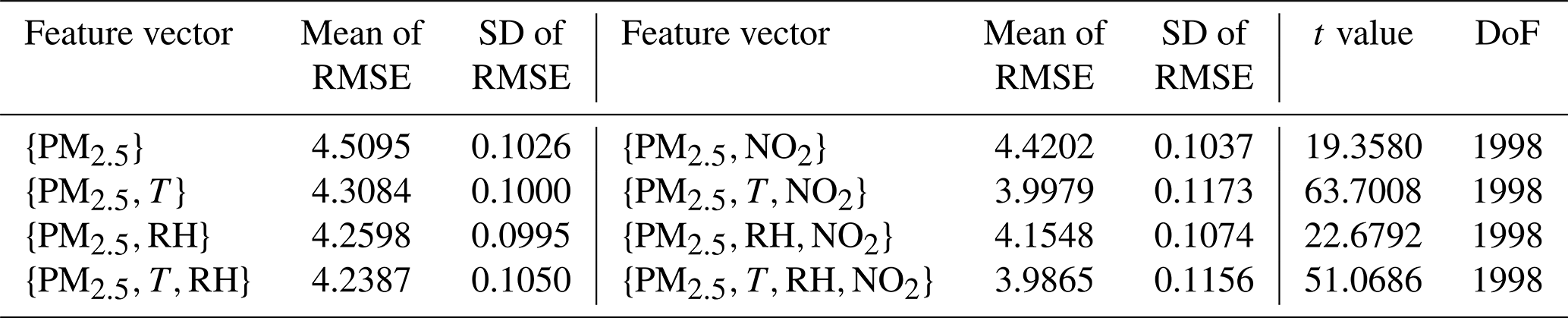
We performed an uncertainty analysis of the MLR-based calibration model by using a bootstrapping technique on a test dataset. Table 12 shows the statistics of uncertainty analysis for each feature vector and t values between two feature vectors whose difference is the existence of NO₂. We selected eight feature vectors with various independent variables to verify whether the addition of NO₂ affects the performance of our calibration model. The four feature vectors we considered are PM_2.5, PM_2.5, T, PM_2.5, and RH and PM_2.5, T, and RH. We also added NO₂ to create four other feature vectors, namely PM_2.5, NO₂, PM_2.5, T, NO₂, PM_2.5, RH, and NO₂ and PM_2.5, T, RH, and NO₂. We generated 1000 test sets using a bootstrapping technique with replacement. We evaluated mean and standard deviation values of RSMEs calculated over 1000 test sets for each feature vector. In addition, we applied a t test to verify the effectiveness of adding NO₂ to each feature vector. Consideration of NO₂ additionally reduces mean values of RMSE for all four feature vectors. Contrarily to the mean value, the standard deviation of RMSE values for every feature vector increases slightly with the addition of NO₂. We evaluated the t value for the mean values of RMSE for two feature vectors, with and without NO₂; for example, the t value between PM_2.5 and PM_2.5 with NO₂. Hence, we can evaluate four t values. The degree of freedom (DoF) is 1998, so the relevant p values are much less than 0.00001. Therefore, the difference in the mean RMSE values of the PM_2.5-included and PM_2.5-excluded groups is significant. From these results, we can conclude that the performance of the MLR-based calibration model can be enhanced with consideration of PM_2.5 concentrations.

Table 12 Statistics of uncertainty analysis in relation to selected feature vectors and t values.

4 Conclusions

The factors directly affecting the performance of a low-cost PM sensor, including temperature, relative humidity, and particle composition, have been scrutinized for their impact on sensors' performance enhancement. Additionally, this study investigated the potential of NO₂, a precursor gas that gives rise to PM_2.5 through atmospheric chemical reactions, to improve the performance of the calibration model. To this end, we used the PurpleAir PA-II unit, which contains two Plantower PMS 5003 sensors, as a low-cost PM_2.5 sensor. The PA-II units need to be typically installed close to reference monitoring sites measuring PM_2.5 concentrations and other pollutants, such as NO₂, in order to analyze their calibration. We identified an EPA-certified monitoring instrument whose deployed location is within close proximity to the installed location of 14 PA-II units, which satisfied the condition for co-location with a reference monitoring site. The monitoring site is located in Rubidoux, CA, USA. A study period of 2 years, i.e., from January 2018 to December 2019, was selected to include all seasons. Two units among 14 PA-II units were selected based on the availability of 23 months or more of measurement data from each PA-II unit, as well as their low intra-model variability through correlation analysis.

One of the two selected PA-II units was compared to FRM and BAM-1020 instruments based on daily and hourly PM_2.5 measurements. A comparison of the BAM-1020 instrument with the FRM instrument was also conducted on a daily PM_2.5 measurement basis to evaluate the performance of the BAM-1020. The BAM-1020 instrument had a slope of 0.923, an intercept of 0.741, and an R² of 0.896 compared to the FRM instrument, which implies that it provides an acceptable performance as a reference monitor for the calibration of low-cost PM_2.5 sensors. For a PA-II unit, the Pearson correlation coefficient against the BAM-1020 instrument was shown to be 0.928 on an hourly basis. The per-month analysis was conducted on hourly PM_2.5 measurements of the PA-II unit against the BAM-1020. Results showed that the PA-II unit has a good correlation during the winter season, i.e., November, December, and January, with an R² value between 0.819 and 0.906, but a lower correlation during other months. The performance of the PA-II units was not notably affected by temperature or relative humidity (RH) during the winter months. Temperature and/or RH were found to improve R² during June and July 2018, but this effect in 2019 was not the same as in 2018.

A per-month analysis showed that NO₂ is a key factor that increased the value of R² during September 2018 and August and September 2019. The effect of the addition of NO₂ for the calibration of PA-II units was much larger when RH and temperature were considered together. In particular, NO₂ was shown to have more effect during months when the performance of PA-II units is moderate. It is expected that NO₂ can be used to improve the performance of low-cost PM_2.5 sensors, but the effect of NO₂ should be further investigated for various ambient conditions.

Two methods for calibrating PA-II units, the multiple linear regression (MLR) and random forest (RF), were evaluated on a test set of 1 year of data. We considered additive and multiplicative terms in two calibration methods. The RF method yielded better performance than the MLR method because it provides a larger R², as well as smaller RMSE and MAE when NO₂, referred to as collocated NO₂, measured from the collocated monitoring site was not used for calibration. However, when collocated NO₂ is considered, MLR models showed similar performance to RF models. When several features, such as PM_2.5, temperature, RH, NO₂, and their multiplicative terms, are considered together to calibrate PM_2.5 measurement data using the MLR method, the calibration performance was shown to increase remarkably compared to cases where only PM_2.5 was considered. For instance, the RMSE value decreased from 4.513 to 3.912 µg m⁻³. In RF models with collocated NO₂, the inclusion of temperature and RH improved R², RMSE, and MAE by an increase of 0.018, a decrease of 0.172, and a decrease of 0.119 µg m⁻³, respectively, compared to the best RF models without NO₂. Contrarily to the MLR model, multiplicative interaction terms do not affect calibration performance with a certain direction compared to those without NO₂; some combinations of features provide slight enhancement, while the others cause worse performance.

We showed that NO₂ data could improve calibration performance in both MLR and RF models. The NO₂ data we referred to were measured from an expensive reference monitor and are very reliable. However, it is not always feasible to have an NO₂ instrument with high accuracy collocated with a low-cost PM sensor. An alternatives is to use low-cost NO₂ sensors. However, their performance remains questionable. To solve this issue, we investigated the effectiveness of using NO₂ measurements collected from distant reliable NO₂ monitoring sites, called distant NO₂, whose locations are not that far from a low-cost PM_2.5 sensor. It was demonstrated that distant NO₂ is effective for calibration models based on the MLR and RF algorithms when distant NO₂ has a high correlation with collocated NO₂. Furthermore, we showed that the MLR method can achieve a similar calibration performance compared to the RF method when reliable distant NO₂ is considered.

We performed an evaluation of different PA-II units and found that incorporating NO₂ significantly enhanced calibration performance across different PA-II units. This consistency held even when using models trained with different sensors at the same location, reinforcing the reliability of generating consistent data across these units. Additionally, the uncertainty analysis underscored a substantial performance boost by including NO₂ in the MLR method, showing a marked difference compared to its omission.