Identification of ice-over-water multilayer clouds using multispectral satellite data in an artificial neural network

An artificial neural network (ANN) algorithm, employing several Aqua MODerate-resolution Imaging Spectroradiometer (MODIS) channels, the retrieved cloud phase and total cloud visible optical depth, and temperature and humidity vertical profiles is trained to detect multilayer (ML) ice-over-water cloud systems identified by matched 2008 CloudSat and CALIPSO (CC) data. The trained multilayer cloud-detection ANN (MCANN) was applied to 2009 MODIS data resulting in combined ML and single layer detection accuracies of 87 % (89 %) and 86 % (89 %) for snow-free (snow-covered) regions during the day and night, respectively. Overall, it detects 55 % and ∼ 30 % of the CC ML clouds over snow-free and snow-covered surfaces, respectively, and has a relatively low false alarm rate. The net gain in accuracy, which is the difference between the true and false ML fractions, is 7.5 % and ∼ 2.0 % over snow-free and snow/ice-covered surfaces. Overall, the MCANN is more accurate than most currently available methods. When corrected for the viewing-zenith-angle dependence of each parameter, the ML fraction detected is relatively invariant across the swath. Compared to the CC ML variability, the MCANN is robust seasonally and interannually and produces similar distribution patterns over the globe, except in the polar regions. Additional research is needed to conclusively evaluate the viewing zenith angle (VZA) dependence and further improve the MCANN accuracy. This approach should greatly improve the monitoring of cloud vertical structure using operational passive sensors.

1 Introduction

Passive remote sensing with polar-orbiting and geostationary passive imagers is currently the only approach suitable for nearly continuous monitoring of clouds day and night around the globe. While cloud remote sensing is well established and the methodologies are abundant (e.g., Stubenrauch et al., 2013), detecting and characterizing multilayered clouds remain a continuing challenge. Typically, algorithms employed to retrieve properties, such as cloud optical depth or phase, treat the radiances for a given cloudy imager pixel as emanating from a single plane-parallel cloud sheet. Rarely, if ever, will an actual cloud entirely satisfy the plane-parallel assumptions. Instead, the sizes and densities of the hydrometeors vary vertically and horizontally within the atmospheric column corresponding to a cloudy imager pixel. The top and side surfaces of clouds, even stratus, typically have bumps and troughs that deviate to various degrees from the uniformity implicit in the plane-parallel model (e.g., Loeb and Coakley, 1998). Simply having vertical extent can cancel the plane-parallel assumption when viewing parts of a cloud side (e.g., Liou and Ou, 1979). Multilayered clouds also violate the model.

Accounting for variations in single-layer-cloud morphology with a non-plane-parallel type of model is too complex for use in operational retrieval algorithms and likely requires information that is currently unavailable in most imager radiance datasets. Moreover, radiative transfer calculations used in weather and climate models are based on the same plane-parallel premise, although methods are being developed to account for some 3D structure (e.g., Schäfer et al., 2016). For single-layer (SL) clouds, the nonuniform geometry is the predominant deviation from the plane-parallel ideal. It mostly affects retrievals of cloud optical depth (COD), cloud-particle effective radius (CER), and, to a lesser extent, inferences of cloud-top phase and cloud-top height (CTH). The presence of two water phases and separation of the upper and lower layers in ice-over-water multilayer (ML) systems can also produce large errors in COD and CER and significantly diminish the accuracies of thermodynamic phase and cloud-top height (CTH) retrievals (e.g., Minnis et al., 2007; Yost et al., 2023). Reducing uncertainties in the retrievals due to nonconformance with the SL plane-parallel ideal, particularly for ML clouds, is critical to increasing the value of imager cloud retrievals for a variety of applications.

Reliable determination of cloud characteristics is critical to the Clouds and the Earth's Radiant Energy System (CERES; Loeb et al., 2016) for converting broadband radiance measurements to reliable shortwave and longwave fluxes at the top of the atmosphere, within the atmosphere, and at the surface. Cloud properties extracted from satellite imagery are also exploited in a wide variety of applications. These include, among others, verifying climate model cloud parameters (e.g., Zhang et al., 2005; Stanfield et al., 2014), enhancing aviation safety (Mecikalski et al., 2007; Smith et al., 2012), improving short-term weather forecasts (e.g., Kurzrock et al., 2019; Benjamin et al., 2021), and estimating surface radiative fluxes (e.g., Rutan et al., 2015; Ryu et al., 2018). All of these applications and others (e.g., Chen and Zhang, 2000; Kato et al., 2019; Morcrette and Christian, 2000) will benefit from more accurate cloud properties, especially for ML systems.

Active instruments such as the Cloud-Aerosol LIdar with Orthogonal Polarization (CALIOP) lidar on the Cloud-Aerosol Lidar and Infrared Pathfinder Satellite Observations (CALIPSO) satellite (Winker et al., 2009) and the Cloud Profiling Radar (CPR) on CloudSat (Stephens et al., 2008) together have produced the most detailed depictions of cloud vertical structure on a global scale. These satellites are part of the A-Train, the Afternoon Constellation of Sun-synchronous orbiters that, for years, flew nearly the same tracks (13:30 equatorial crossing time) separated by only a few minutes. Other satellites with imagers, particularly Aqua with the MODerate-resolution Imaging Spectroradiometer (MODIS), are also members of the A-Train. The CALIOP and the CPR are both near-nadir-viewing instruments that generate profiles of atmospheric particles only in a narrow curtain along the satellite track. Those profiles, which often include overlapping clouds, are valuable for many uses, especially when combined with other instruments on the A-Train. Because they sample only a tiny fraction of the globe at two local times each day, the current active instruments have limited utility for many of the applications served by operational satellite imager products.

Efforts to accurately identify and unscramble ML clouds from passive imagery have yielded a variety of methods that have either been demonstrated as efficacious or are being applied routinely. They are based on interpreting radiances from either multiple instruments or from a single instrument with multiple channels. To identify ML clouds, Lin et al. (1998) matched microwave radiometer (MWR) retrievals of cloud liquid water path (LWP) from polar-orbiting satellites with retrievals of COD from geostationary satellites. Minnis et al. (2007) used MWR retrievals of LWP matched with imager retrievals of COD and CER to detect and retrieve ML cloud properties over water surfaces. By combining Aqua MODIS cloud-top pressure (CTP) and COD with the optical centroid cloud pressure retrieved from the Ozone Monitoring Instrument on the Aura satellite, Joiner et al. (2010) discriminated between vertically extended and ML clouds.

The single-instrument approach, which is more viable for monitoring ML clouds from a greater number of satellites, often relies on discrepancies between the visible (VIS, ∼ 0.65 µm) channel COD and that determined from other channels. For example, COD derived from infrared radiances is limited to values of less than ∼ 5 because the usable signal diminishes for thicker clouds. Thus, the two COD retrievals can be used to detect thin cirrus over a thicker lower cloud. Pavolonis and Heidinger (2004) identified ML clouds by comparing the COD retrieved from the brightness temperature differences from the 11 and 12 µm channels, BTD₁₁₁₂, with the VIS COD. They suggested that the MODIS 1.38 and 1.63 µm reflectances could be combined with BTD₁₁₁₂ to retrieve the cirrus optical depths for comparison with the VIS COD. The MODIS CO₂ channels were used by Chang and Li (2005) to retrieve IR COD for ML cloud detection. Their method was simplified by Chang et al. (2010) to employ brightness temperatures from CO₂ and 11 µm channels to identify high clouds and ultimately to detect ML clouds in the CERES MODIS Edition 4 products (CM4; Minnis et al., 2021). Similarly, Wind et al. (2010) contrasted the cloud-top pressure (CTP) derived with a CO₂ method to that based on absorption in the MODIS 0.94 µm channel along with other tests to identify ML clouds in MODIS pixels. To further improve ML detection, this technique was enhanced with additional tests, including the Pavolonis and Heidinger (2004) method (Platnick et al., 2017; Marchant et al., 2020).

Desmons et al. (2017) exploited multi-angle polarized spectral reflectances and two different retrievals of CTP from the POLarization and Directionality of the Earth's Reflectances (POLDER) instrument on another A-Train satellite. Instead of using COD retrievals, Wang et al. (2019) utilized a series of tests applied to three spectral reflectances and two infrared brightness temperatures measured by the Visible Infrared Imaging Radiometer Suite (VIIRS) to classify clouds as single-layer ice or water, multilayer, probable multilayer, or uncertain phase and layering. Their technique yielded results similar to those from Platnick et al. (2017). For detecting ML clouds in VIIRS data, CERES replaced the CO₂ channel with the 12 µm channel in the Chang et al. (2010) approach. It found fewer ML clouds than the method using the CO₂ channel (Minnis et al., 2023).

These physically based approaches to ML detection are limited in many respects by a priori knowledge and ambiguous spectral signals in the imager radiance complement, problems that affect many cloud remote sensing approaches. To minimize these limitations, artificial neural networks (ANNs) are increasingly employed to characterize clouds from passive imager data. By training with a select set of relevant input parameters and a known output value, the ANN has the potential to better interpret several subtle, but often ambiguous radiative signals that are difficult to reconcile in physically based retrievals. Kox et al. (2014) and Strandgren et al. (2017) employed an ANN to determine cirrus COD and CTH, while Cerdeña et al. (2007) used it to estimate liquid water cloud COD and CER, and Taravat et al. (2015) detected the presence of clouds with it. Using an ANN, Minnis et al. (2016) retrieved thick ice cloud COD at night and Håkansson et al. (2018) more accurately determined CTP and CTH than available physical methods. Stengel et al. (2020), Wang et al. (2020), and White et al. (2021) use ANNs for cloud detection and phase discrimination. Machine learning techniques were employed by Haynes et al. (2022) to detect low clouds in both single- and multilayered conditions for geostationary satellites. Tan et al. (2022) found that a random forest technique was highly accurate in detecting multilayered clouds from geostationary satellite imager data. These and other examples have clearly demonstrated that ANNs have significant potential for advancing the characterization of global cloudiness from passive imager radiances.

To improve the CERES ML detection, Sun-Mack et al. (2017) developed a multilayer cloud detection ANN (MLANN) to distinguish between SL and ML clouds using MODIS radiance data matched to CALIPSO and CloudSat vertical profiles of clouds over snow-free surfaces. The MLANN was trained separately for day and night data. Minnis et al. (2019) enhanced the MLANN by including more input parameters and additional output variables such as upper layer CTH, COD, and cloud-base height (CBH). They also used only high-confidence CloudSat and CALIPSO data for training and further trained the MLANN separately for clouds identified as either ice or water phase by the CERES CM4 algorithms. Using 1 month of data, they found that, for nonpolar clouds, the MLANN correctly identified ML and SL clouds together 80.4 % and 77.1 % of the time during day and night, respectively, using CALIPSO data averaged over an 80 km distance. Those values are 5 % greater in absolute terms than their earlier counterparts. While the accuracies are quite encouraging, the approach needs further refinement and complete seasonal and global coverage.

This paper reports on the continued development of the MLANN to detect ML clouds. Revisions to the previous training are made using newer versions of CALIPSO and CloudSat products with constrained horizontal resolution. To be more representative of its use and avoid confusion with other machine-learning terms, the acronym for this revision is changed from MLANN to the multilayer cloud-detection artificial neural network, MCANN. To expand coverage to the entire globe, the MCANN is trained separately for CERES ice- and water-cloud pixels separately for both snow-free and snow/ice-covered surfaces using an entire year of data. Input to the MCANN is also enhanced with some new variables. Finally, because the MCANN is trained with near-nadir data, its utility for full-swath MODIS data is examined.

2 Data

The MCANN is trained with input taken from Aqua MODIS imager data and cloud products, as well as numerical weather model reanalyses. Different datasets are used for daytime and nighttime. Daytime corresponds to all measurements taken when the solar zenith angle (SZA) is < 82°. Active sensor data serve as the output.

2.1 C3M and MODIS

MODIS on Aqua, the CALIOP, and the CPR took measurements continuously within ±3 min of each other over a given location until 2011, when CloudSat suffered battery problems and thereafter only collected data during the day. CloudSat exited the A-Train during February 2018. The CALIOP and the CPR were aligned to view nearly the same area along their respective orbits. Because their flight tracks are typically close to the Aqua nadir path, MODIS scans the same scene at viewing zenith angles of VZA < 18°. Vertical profiles of clouds from the CALIPSO Version 4 (Vaughan et al., 2022) and the CloudSat 2B-CLDCLASS_R05 (Sassen and Wang, 2008), 2B-CWC-RO (Austin et al., 2009), and 2C-ICE (Deng et al., 2015) datasets were collocated with 1 km Aqua MODIS Collection 6.1 radiances and CERES-retrieved cloud properties to produce an updated version of the CloudSat, CALIPSO, CERES, and MODIS (C3M) product (Kato et al., 2010). The C3M also includes CERES MODIS cloud properties, such as cloud-top phase, cloud-particle effective radius (R_CM), and COD (τ_CM), which were retrieved from the MODIS radiances using an interim CERES Edition 5 algorithm, CM4+. Those retrievals assumed that all of the clouds were single-layered.

The CM4+ methodology is the same as that of the CM4 algorithms except for two changes. In CM4+, τ_CM is retrieved over snow and ice surfaces using a combination of 1.61 and 1.24 µm reflectances, as suggested by Minnis et al. (2021). The former channel is used for thinner clouds (COD < 8 for ice clouds, COD < 32 for water clouds) and the latter for thicker clouds. The Aqua MODIS 1.6 µm channel consists of 10 sensors. Of those 10, only 6 operate properly. To obtain full 1.6 µm imagery, the 1.6 µm reflectance for each bad pixel was replaced with that from the nearest good detector. That method was applied to the 101-pixel-wide MODIS swath of the C3M. The other change for CM4+ is the use of the two-habit ice crystal model of Loeb et al. (2018) for retrieving ice-cloud properties.

A separate dataset is the full-swath Aqua CM4+ cloud product and the Aqua MODIS Collection 6.1 radiances, which are sampled every other scan line and every fourth pixel. Note that the 1.6 µm channel is only available from 3 of the 5 sensors on the CERES-sampled Aqua MODIS Collection 6.1 data. The corrections applied to faulty 1.6 µm sensors for C3M have not yet been implemented for CERES Aqua MODIS data prior to 2019. Therefore, the sampling is reduced, and all data from the faulty sensors are excluded in the full-swath 2009 and 2013 data.

To produce a complete vertical profile of cloud-filled layers in a given pixel, the C3M converts the CloudSat CLDCLASS high-confidence cloud profiles from 240 to 60 m vertical resolution and then merges them with the CALIPSO cloud profile and vertical feature mask (VFM). The nominal horizontal footprint of a CALIOP shot at the Earth's surface is 330 m in diameter. To detect fainter clouds, the CALIPSO processing system computes horizontal averages (HA) of the lidar signals from multiple shots corresponding to increasing distances along the track: 1, 5, 20, and 80 km. The last three HA values are for altitudes above 8 km. This analysis uses only those clouds detected at HA ≤ 5 km to define the cloud profiles, because nearly all of the clouds identified solely at lower resolutions had COD < 0.1. Since the CM4 detection rate drops significantly for those extremely small optical depths (Trepte et al., 2019), few of those cirrus clouds are discernible and are less likely to be identified in ML conditions. Additionally, in the previous formulation (Minnis et al., 2019), all three CALIPSO 0.33 km pixels matched to a given MODIS pixel were required to be cloudy after the horizontal averaging was performed. Here, only two out of three 0.33 km pixels are required to be cloudy and any cloud having τ_CM< 0.5 is assumed to be single-layered. The latter constraint assumes that the ML signal from such optically thin clouds is negligible, and any retrieval attempt will yield upper and lower cloud-layer properties that are, at a minimum, highly uncertain. To perform additional analyses, the CC COD (τ_CC) was computed for each ice-layer pixel identified as ML in the CALIPSO-CloudSat profiles. The value of τ_CC is equal to the CALIPSO ice COD, when the CALIOP signal shows a return from the lower layer cloud; otherwise, it is equal to the combined CALIPSO-CloudSat COD. To cover all seasons for snow-free surfaces and facilitate computer processing for training, the C3M data were sampled every fourth pixel of 2008 for snow/ice-free (SF) areas, while all pixels were used for the snow/ice-covered (SC) scenes. This full-year training set is more comprehensive than the 1 month dataset of Minnis et al. (2019). The complete, up-sampled 2009 C3M data were employed as an independent dataset for validating the MCANN.

The C3M data were merged with the relevant surface skin temperature and vertical profiles of relative humidity taken from the CERES Meteorology, Ozone, and Aerosol (MOA) product (Gupta et al., 1997). The latest MOA product is the result of regridding and interpolating spatially and temporally the version 5.4 reanalysis produced by the Global Modeling Assimilation Office Global Earth Observing System (GEOS-5.4), an update of the versions described by Rienecker et al. (2008). These are the same data employed in the CM4+ retrievals.

2.2 Input variables

The MODIS input variables are listed in Table 1. Both daytime and nighttime MCANN inputs include latitude, longitude, surface type (land or water), surface elevation, brightness temperatures T_λ, and brightness temperature differences, BTD${}_{\mathit{\lambda }\mathrm{1}\mathit{\lambda }\mathrm{2}}=T_{\mathit{\lambda }\mathrm{1}}-T_{\mathit{\lambda }\mathrm{2}}$, where λ is the wavelength in µm abbreviated to the first two digits. Here, brightness temperatures at 3.7, 6.7, 8.5, 11, 12, and 13.3 µm are used together with BTD₃₇₁₁, BTD₆₇₁₁, BTD₈₅₁₁, BTD₁₁₁₂, and BTD₁₁₁₃. The parameters involving the 13.3 µm channel were not used over snow-covered surfaces because of striping in the 13.3 µm images over Greenland and Antarctica. Also included are τ_CM and the GEOS-5.4 input data. During the day, τ_CM is retrieved using solar reflectances and corresponds to the total cloud optical depth. At night, it is estimated from three infrared channels and typically represents the uppermost cloud COD (e.g., Minnis et al., 2021). Nocturnal values exceeding ∼ 5 are often not very accurate but serve to indicate that the cloud is not optically thin. The GEOS input data comprise the surface skin temperature and the relative humidities at the surface and at 850, 700, 500, 400, 300, 200, and 100 hPa. Relative humidity can indicate the presence of a cloud at a given altitude depending on the quality of the source (e.g., Minnis et al., 2005).

Table 1 Input parameters for the MCANN.

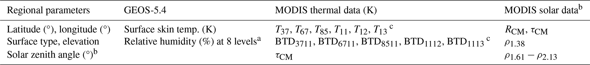
^a Levels: surface, 850, 700, 500, 400, 300, 200, 100 hPa. ^b Day only. ^c Snow/ice free only.

During the day, the additional input data consist of the SZA, the 1.38 µm reflectance (ρ_1.38), and the reflectance difference between 1.6 and 2.1 µm, ρ_1.61−ρ_2.13. CM4+ retrievals of R_CM are also employed for the MCANN formulation. The reflectances and R_CM were not used by Minnis et al. (2019).

2.3 Output: single or multilayered

According to Kato et al. (2010), approximately 51 % of cloud systems identified by the CPR and CALIOP consist of two or more layers separated by at least 200 m. Of that 51 %, atmospheric columns having 2, 3, 4, 5, and 6 plus layers account for 57 %, 28 %, 10 %, 4 %, and 1 % of the pixels, respectively. Those statistics include liquid-over-liquid, ice-over-ice, water-over-ice, and ice-over-water cloud overlap. Unscrambling this variety of layering is a daunting task.

To simplify ML detection and later retrievals, only those clouds having the greatest differences in properties are assumed to be multilayered. Thus, only systems having ice-over-liquid clouds are considered; this is because they differ in phase, scattering properties, and altitude and are more common than liquid-over-ice clouds. Thus, multilayered clouds are defined here as any combination of ice-cloud layers above one or more water cloud layers with the constraint that the top of the uppermost water layer must be at least 1 km below the bottom of the lowest ice-cloud layer. All ice-cloud layers together are considered to constitute a single cloud layer. Similarly, all liquid layers are considered together as a single layer.

Selection of 1 km as the minimum separation distance is based on the need to ensure complete separation between the ice and water layers and to maximize the number of detected ML clouds. Using a smaller separation would likely diminish detection accuracy significantly, as demonstrated by Tan et al. (2022). Sun-Mack et al. (2017) and Minnis et al. (2019) found that a larger separation distance can result in greater accuracy but at the expense of missing a significant number of actual ML clouds.

An ice-cloud layer is assumed to be present in the profile if

• 1.

  the CALIPSO VFM cloud phase is either ice clouds or mixed-phase clouds, or

• 2.

  at least one layer with extinction occurs at a height above the altitude corresponding to 253 K and no temperature inversion exists in the atmospheric layer between the altitudes corresponding to 273 and 253 K; this constraint is used to eliminate the possibility of warm clouds occurring above the assumed ice threshold of 253 K.

For training, all C3M pixels having an ice-cloud layer over a water cloud layer are assigned an output value of 1, while all other cloudy pixels are assumed to be single-layered and are assigned a value of 0.

3 Methodology

The MCANN is trained using the MathWorks Patternnet software (https://www.mathworks.com/help/deeplearning/gs/pattern-recognition-with-a-shallow-neural-network.html, last access: 23 May 2024). The scaled conjugate gradient training function was employed here because it seemed best suited to handling very large training datasets with many iterations. This is a switch from the Levenberg–Marquardt method used in the MLANN. Only one hidden layer is used for this shallow neural network. It was found that a second layer yielded no significant increase in accuracy but greatly increased training time. Each layer employed the logarithmic sigmoid and hyperbolic tangent sigmoid functions (logsig, transig) as the activation type. In the hidden layer, the number of neurons varies from 50 to 70 depending on the data category (e.g., snow-free daytime ice clouds). The exact number was determined by adding neurons until gains in accuracy ended. An epoch of 2000 was used for ending the fitting but it was not always reached. Mean squared error was used to measure performance. For final training, the sampled 2008 data for each category were divided into 60 %, 20 %, and 20 % each for training, testing, and validation, respectively. All other training parameters are determined by the Patternnet program.

To avoid local minima in the neural network, the training runs were repeated many times using different samplings of the dataset (e.g., every third pixel or every fifth pixel); different random initial weights; and various percentages for training, testing, and validation. Local minima were identified when the training convergence time was abnormally short or long. Overfitting was avoided by using a very large dataset (typically more than a million data points), which forces the net to generalize. It was also avoided by using a minimal number of neurons. Additionally, unreasonable data, such as fill values, were filtered out to minimize the noise. A set of range limits was used to eliminate any obviously errant data. Leaving such data in the input set prevents the training from generalizing. Unnecessary input parameters were also removed by trial and error to streamline the training. Finally, similar performances of the MCANN with the 2008 training and 2009 independent validation datasets ensured that the trained network was producing global minima without overfitting.

The input variables in Table 1 were selected by adding in parameters suspected of enhancing ML detectability and computing the accuracy for each addition. If no gain in accuracy occurred, the parameter was not used. Each predictive parameter's influence on the final MCANN formulation was assessed by computing the relative decrease in recall (defined in Sect. 4.1) when a given parameter was removed from the training. The decrease for each parameter was divided by the sum of all of the values to produce a relative ranking of importance. The ranks ranged from 0.038 for BT₁₁ to 0.082 for the relative humidity profiles, which were treated as a single input for these purposes. The second-highest ranked parameter is latitude, followed in the daytime by SZA and ρ_1.38. In general, the brightness temperatures were ranked lower than the BTDs, similar to the rankings reported by Tan et al. (2022) for their random forest method.

Output from the trained MCANN is a probability between 0 and 1 for each pixel. The latter value denotes certainty that the pixel includes ML clouds as defined here. For practical purposes, it is necessary to select a threshold probability above which a pixel is designated as multilayered. A threshold value of 0.5 was chosen based on analysis of the accuracy of the results for probabilities between 0.3 and 0.60. The accuracies (risks) were found to be greatest (least) for thresholds between 0.50 and 0.55.

4 Results

The results presented here consist of comparisons of the MCANN and corresponding CC parameters for the 2008 training dataset along with data from 2009 to ensure robustness of the estimates. Weights and constants were determined by training for each category and parameter and then applied to the independent datasets. The MCANN was trained using the C3M data for the four categories in Fig. 1 to obtain four sets of weights and constants for each surface type.

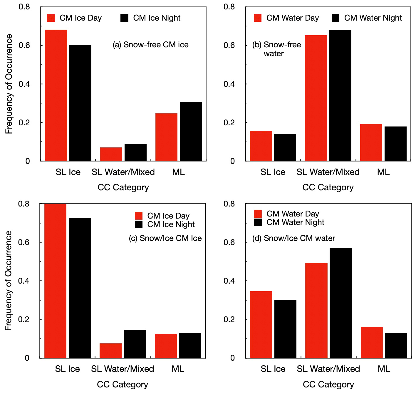
Figure 1 CALIPSO-CloudSat classification frequency of occurrence for matched 2008 CERES-MODIS cloud phase selection, ice (a, c) and liquid (b, d) for snow-free surfaces (a, b) and snow/ice-covered surfaces (c, d).

4.1 Multilayer cloud detection

Figure 2 plots the CC cloud profiles retrieved over six areas during 25 December 2009. The CC layering classification uses gray for SL and blue for ML. In addition to the cloud profiles, the MCANN selection of SL (gray) and ML (blue) is indicated by the lines of dots across the top section of each panel. The surface elevation is denoted by the dashed black line in each panel. On the left are daytime observations over the tropical Atlantic (Fig. 2a), eastern Europe (Fig. 2b), and eastern Antarctica (Fig. 2c). Nocturnal profiles are given on the right for passes over the tropical Indian Ocean (Fig. 2d), the South Pacific (Fig. 2e), and northern Russia (Fig. 2f). In the tropical overpasses, the MCANN detects a large fraction of the ML clouds but also misses a noticeable number of ML pixels. For example, only a few of the intermittent ML clouds between 2.5 and 6.1° N are identified by the MCANN in Fig. 2a and a segment of continuous ML clouds near 12° S in Fig. 2d is missed by the MCANN. Similar results are seen for the midlatitude SF areas, where a few ML clouds are missed around 59° N in Fig. 2b and near 35° S in Fig. 2e.

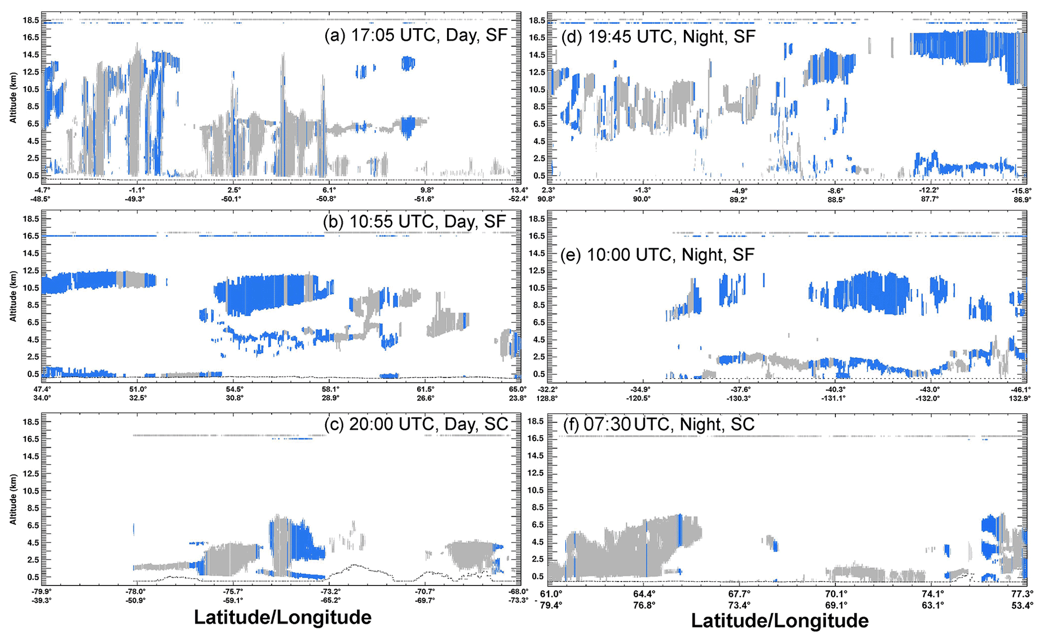
Figure 2 CALIPSO-CloudSat cloud profiles from C3M for 25 December 2009 with CC ML clouds indicated in blue and CC SL denoted in gray. The MCANN ML identification for each profile is indicated as a blue dot at the top of each figure. MCANN SL clouds are indicated with a gray dot. Surface elevation is given as the dotted line at the bottom of each panel. Tropical, midlatitude, and polar cloud profiles are given in the top, middle, and bottom profiles, respectively. SF and SC indicate snow-free and snow/ice-covered surfaces, respectively.

Some false ML clouds are also found in these panels. In Fig. 2b, for example, false ML clouds are evident at 51° N and also in two areas between 56 and 58° N. In the latter case, there are ML clouds in the profile, but they were not classified as such by the CC constraints, possibly due to the 253 K liquid cloud temperature threshold. Thus, some of the false ML may actually be ML clouds. The detection rates for the two SC profiles are much reduced. During the daytime case (Fig. 2c), only one stretch of ML clouds is detected, while even fewer ML clouds are detected at night around 76° N (Fig. 2f). The unidentified ML clouds are more common in both cases.

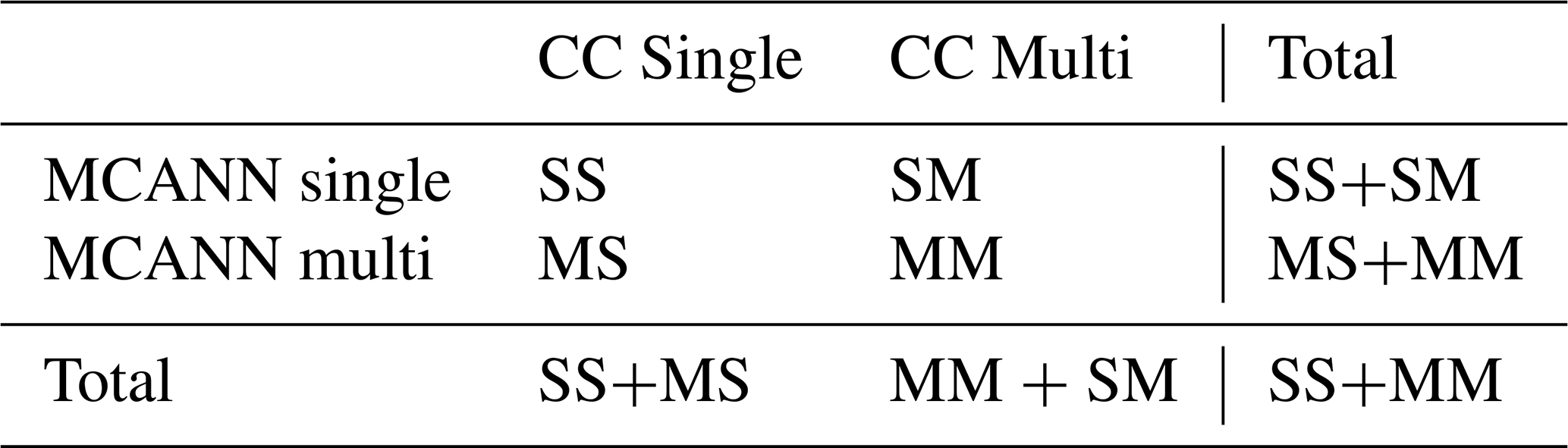
To summarize the results for all of the data, a confusion matrix was constructed for each category. Referring to Table 2, agreement between the MCANN and CC SL classifications is denoted as true positive (SS), while agreement between the ML identifications is defined as true negative (MM). The false SL and ML pixels are given by SM and MS, respectively. Each classification is defined as the number of pixels satisfying the agreement condition divided by the total number of pixels. Those percentages are used to define the following metrics.

$$\begin{array}{}\text{(1)}& {\displaystyle }\text{Accuracy:}\text{ACC}=\text{SS}+\text{MM}.\text{(2)}& {\displaystyle }\text{Real risk:}\text{RR}=\text{MS}+\text{SM}=\mathrm{1}-\text{ACC}.\text{(3)}& {\displaystyle }\text{False ML rate:}\text{FM}=\text{MS}/\left(\text{MS}+\text{MM}\right).\text{(4)}& {\displaystyle }\text{Precision:}\text{PR}=\text{MM}/\left(\text{MS}+\text{MM}\right).\text{(5)}& {\displaystyle }\text{Recall:}\text{RC}=\text{MM}/\left(\text{SM}+\text{MM}\right).\text{(6)}& {\displaystyle }\text{Single-layer confidence:}\text{CoS}=\text{SS}/\left(\text{SS}+\text{SM}\right).\text{(7)}& {\displaystyle }\text{F1 score:}\text{F1}=\mathrm{2}\times \text{PR}\times \text{RC}/\left(\text{PR}+\text{RC}\right).\text{(8)}& {\displaystyle }\text{Net gain of accuracy:}\text{NGA}=\text{MM}-\text{MS}.\end{array}$$

These parameters facilitate the reporting and discussion of the results and the comparisons with other algorithms.

Table 2 Confusion matrix definition.

The results in Table 3, based on the entire 2008 training data, include the confusion matrices for all eight categories with ACC in bold along with the number of CC SL and ML pixels and their sum. During the day, ACC is 84.1 % for CM4 ice clouds over SF areas, with the fraction of ML correctly identified, i.e., RC = 49 %. The classification during the day is a bit better for CM4 liquid clouds: ACC = 88.7 % and RC = 63 %. The real risk for ice clouds is 15.9 % compared to 11.3 % for the liquid clouds. At night the results are similar, although a little worse for ice clouds, with ACC = 81.3 %. However, the ice clouds yield a larger fraction, RC = 55 %, of true ML pixels than during the day. Fewer ML clouds are found for liquid clouds at night. More of the ML clouds are classified as ice because the nocturnal cloud temperature retrieval is based strictly on infrared radiances (Yost et al., 2021, 2023). Nevertheless, ACC is the same for both times of day for liquid-phase clouds. At night, RR for ice clouds increases to 18.7 % and drops slightly for water clouds. A total of ∼ 12 million pixels was used in the SF training.

Table 3 Confusion matrices (each bounded by vertical lines) for MCANN applied to Aqua MODIS relative to layer identification from CloudSat-CALIPSO, 2008, from the training set. The bold numbers indicate the percent correct for each matrix. The bottom row of each matrix indicates the number of CC pixels for each category.

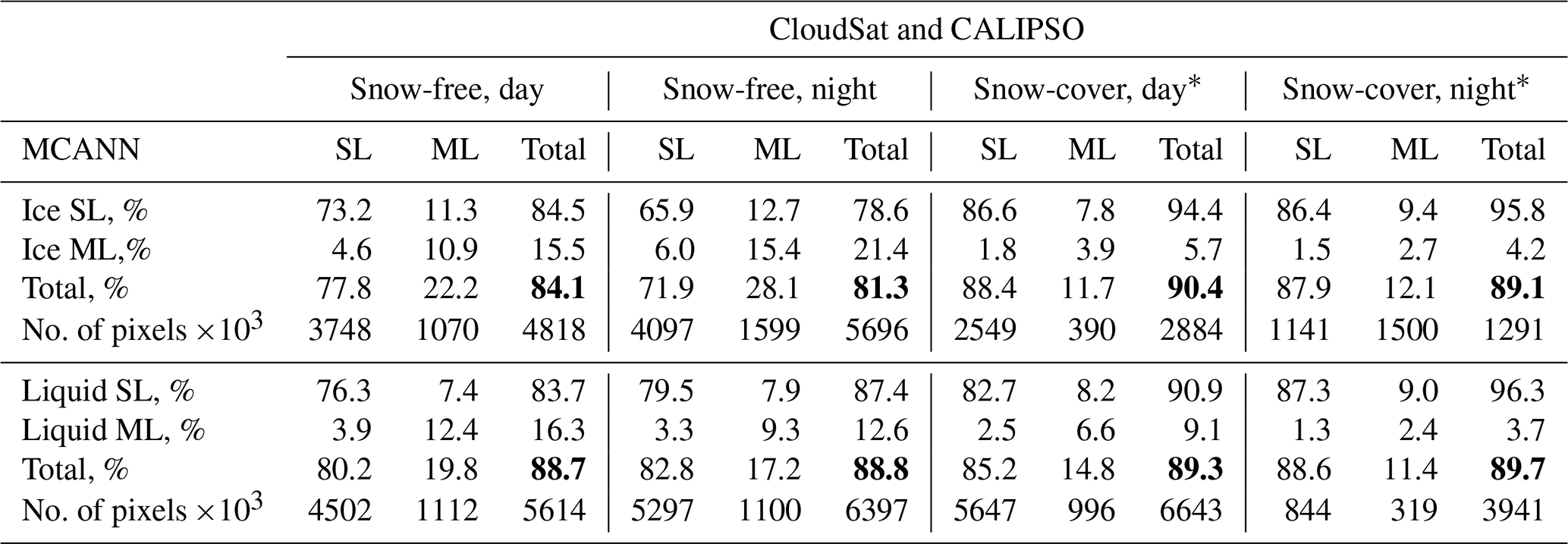
As suggested by Fig. 2, the efficacies of the MCANN for detecting ML clouds over snow-covered areas are considerably reduced relative to their snow-free counterparts. While the ACC values are actually greater than those during the day (Table 3), recall drops to 35 % and 45 % for ice and liquid clouds, respectively, during the day. The fraction detected, RC∼ 22 %, is even lower at night. Nevertheless, because fewer pixels qualify as ML clouds over SC surfaces, according to the definition used here, the MCANN RR values are smaller than those over SF surfaces. It is notable that, for both SF and SC surfaces, the ML false alarm rate is less than 55 %.

4.2 Independent evaluation

The results from the training are encouraging, but they are not based on an independent dataset. To evaluate the robustness of the MCANN, all 2009 Aqua MODIS data were processed with the trained algorithm. In general, the statistics for the eight categories are all very similar to those in Table 3. To summarize the effectiveness of the MCANN, the 2009 ice and liquid ML results for the SF/SC and day/night categories are combined in Table 4. Over SF surfaces, ACC is 87.0 % and 85.6 % for day and night, respectively, while the corresponding values over SC surfaces are 89.3 % and 88.7 %. Despite the large ACC values, the MCANN underestimates the ML fraction over SF surfaces by 5.8 % and 4.8 % during night and day, respectively, for the matched CC and MODIS cloudy pixels. A total of 80 million SF pixels were processed, compared to 26 million for SC surfaces. Over SF areas, RR is 13 % for day and 15 % at night. Real risks drop to 11 % for SC regions. It should be noted that the ML fractions reported here are for the number of multilayer MODIS pixels divided by the total number of cloudy matched CC and MODIS pixels. Since the CERES MODIS mean cloud fraction is ∼ 0.66, the actual fraction of MODIS pixels that are classified as ML would need be multiplied by 0.66.

Table 4 Same as Table 3, but for combined liquid and ice results from applying MCANN to the 2009 validation dataset. The bold numbers indicate the percent correct for each matrix.

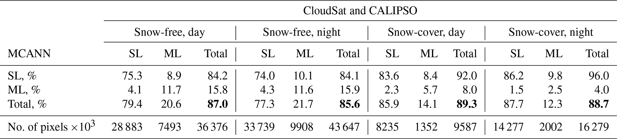
The net gain of accuracy relative to the SL assumption is an important parameter to consider in any ML detection scheme. Using the SL assumption in cloud retrievals, the accuracy would be equal to the sum of SS and MS. Introducing a multilayer detection method yields both false and true ML pixels. Thus, a new source of error comes with the additional information. The net gain of accuracy is not simply equal to ACC – SS; it must account for the newly introduced error, represented in MS. The falsely detected ML clouds are a potentially worse source of error than the SL assumption for ML clouds. Multilayered cloud property retrievals for a false ML pixel require the creation of a second cloud layer and inference of its properties, whereas a single-layered retrieval for a true ML pixel results in a cloud with properties somewhere between the upper and lower layer. Thus, including a ML detection algorithm in a retrieval may not be reasonable if FM is too large. Based on Table 4, the MCANN NGA = 7.6 % and 7.3 % during day and night, respectively, over SF surfaces. The corresponding values over snow-covered surfaces are 3.4 % and 1.0 %. While the MCANN provides a nearly negligible amount of information over SC areas at night, elsewhere it clearly represents an improvement over simply assuming that all clouds are single-layered.

Global distributions of the mean 2009 ML cloud fraction from the validation results are plotted in Fig. 3. While the daytime MCANN means (Fig. 3c) are noticeably smaller than the average CC ML fractions (Fig. 3a), the two datasets have similar distributions. At night (bottom), the patterns are much like those during the daytime, except in the polar regions. More CC pixels (Fig. 3d) are classified as ML in the tropics than during the daytime. A comparable increase occurs in the MCANN nocturnal results (Fig. 3d), which have ML fractions over much of the Amazon Basin and central Africa that are comparable to their CC counterparts, although they are smaller elsewhere. As expected from Table 4, the MCANN ML fractions in the polar regions are relatively small during the day and negligible at night. Figure 3c and d show the ML fractions determined from all of the positive ML detections from the MCANN, whether they are correct or not. Figure 3e and f show the corresponding distributions of ML fractions based only on pixels that are actually correct according to the matched CC data. As expected from Table 4, the magnitudes for both day and night are significantly reduced compared to those for all of the MCANN results. The relative distributions of the correct values are similar to their all-MCANN counterparts.

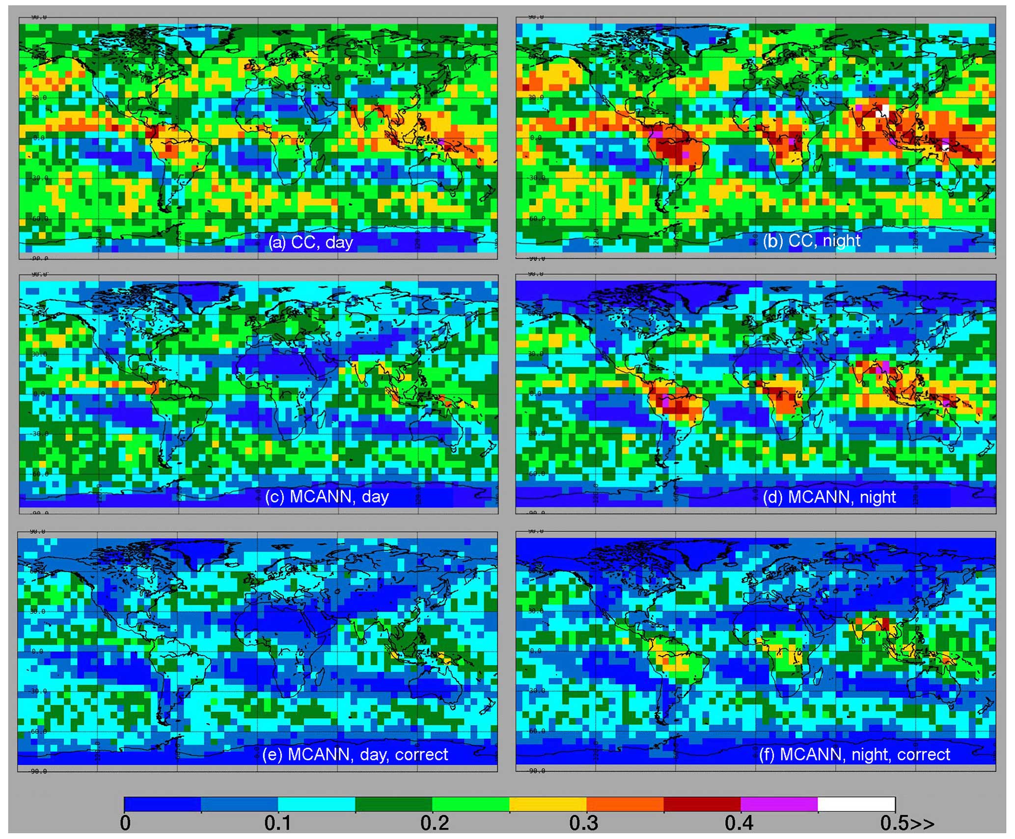
Figure 3 Fraction of matched 2009 CC and Aqua MODIS pixels classified as multilayer clouds. CALIPSO-CloudSat and Aqua MODIS MCANN ML classifications on panels (a), (b), and (c), (d), respectively. Correct MCANN ML cloud fractions shown at panels (e) and (f). (a, c, e) Day and (b, d, f) night pixels, respectively.

The latitudinal variations of the mean ML fractions are plotted in Fig. 4. As expected from Fig. 3, the zonal patterns are much the same with the MCANN values (triangles) being consistently less than their CC counterparts (circles). In the tropics, the daytime differences generally fall between −0.06 to −0.04 and drop to as low as −0.08 in the polar regions. During the night, the minimum of −0.10 is found over the polar regions, but the differences are comparable to the daytime values between 45° S and 45° N. The MCANN is clearly less effective during the night over snow and ice-covered areas. Overall, the MCANN underestimates the 2009 ML cloud amount by 0.05 and 0.06 relative to the CC ML cloud fraction during day and night, respectively. The nonpolar MCANN zonal night–day ML mean fractional differences from Fig. 4 are plotted against their CC counterparts in Fig. 5 to determine how well the MCANN captures the changes in ML fractions from day to night. The MCANN and CC differences are well correlated as indicated by the squared correlation coefficient, R² = 0.88. While the absolute differences are quite comparable when small, the absolute night–day differences from the MCANN tend to be greater than their CC counterparts at the extremes. The greatest MCANN night–day differences are found in the deep tropics and north of 45° N.

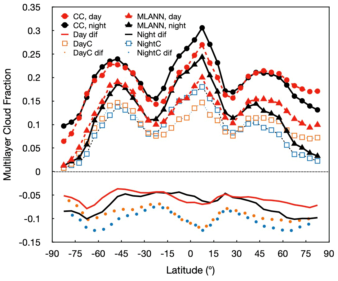
Figure 4 Zonal mean 2009 ML cloud fraction from matched CALIPSO-CloudSat and Aqua MODIS as in Fig. 3​​​​​​​. Zonal differences, MCANN – CC, are also plotted. Global averages are indicated in the legend.

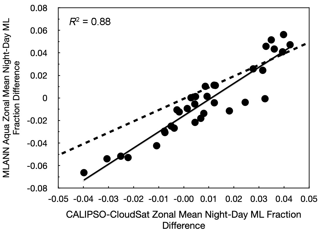
Figure 5 Scatterplot and correlation of MCANN and CC night–day differences in nonpolar zonal mean ML cloud fractions in Fig. 3. Dashed line indicates 1:1 correspondence. Solid line is linear regression fit.

When only the correct MCANN values are considered (open squares), the zonal means drop further below the CC averages. The correct-MCANN differences relative to the CC values, shown at the bottom of Fig. 4, vary zonally much like their all-MCANN counterparts for both day (orange dotted line) and night (blue dotted line) but are 0.02 to 0.07 lower. The sources of these differences are discussed further below.

5 Discussion

These results represent a significant improvement over the MLANN of Minnis et al. (2019), which only attained accuracies of 80.4 % and 77.1 % during the day and night, respectively, over SF surfaces using a single month of data. Over SF surfaces, PR, RC, and F1 from the MCANN are 74 % (72 %), 57 % (52 %), and 64 % (60 %) for daytime (nighttime), respectively. In relative terms, all of those values exceed their MLANN counterparts by 1 % to 20 %. The MLANN NGA values are slightly higher. Much of the increased accuracy of the MCANN relative to the MLANN is due to use of shorter CALIPSO horizontal averaging distances here. By employing CALIPSO averages over distances up to 80 km, Minnis et al. (2019) attempted to detect ML cloud systems that included many cirrus clouds having optical depths smaller than 0.2. Such clouds are difficult to detect with passive remote sensing even when they are single-layered. According to Yost et al. (2021), systems having τ_CC < 0.2 account for ∼ 42 % of all ML clouds for CALIPSO data using HA ≤ 80 km compared to only 18 % for HA ≤ 5 km. A majority of those low-optical-depth ML clouds were not detected in Minnis et al. (2019), resulting in lower accuracies. Typically, cloud identification or multilayered cloud detection methods that use CALIPSO for validation or training have employed data with HA ≤ 1 or ≤ 5 km (e.g., Desmons et al., 2017; Marchant et al., 2020; Tan et al., 2022; White et al., 2021). By using that shorter averaging distance in this study, the fraction of CC ML clouds is ∼ 40 % less than that used by Minnis et al. (2019), but a larger fraction of them is detected. Other sources for the improvement arise from utilizing additional input parameters, including those based on the 13.3 µm channel and ρ_1.38, as well as ρ_1.61−ρ_2.13. Additionally, the assumption that all pixels having τ_CM< 0.5 are automatically SL, regardless of the CALIPSO classification, probably removed some difficult but less important cases.

5.1 Dependence on cloud properties

Much like other retrievals, the MCANN is sensitive to various cloud conditions, such as the altitudes of the two layers and their respective optical depths. Because the MCANN uses a minimum separation distance of 1 km between the ice and liquid cloud layers, the dependence on separation distance is not explicitly considered here. Its impact on MCANN, examined by Sun-Mack et al. (2017) and Minnis et al. (2019), is similar to that from other studies. Tan et al. (2022), for example, found that the probability of ML detection using a random forest method was greatest for separation differences of 3 km or more and that it dropped from values exceeding 0.8 to less than 0.5 for cloud gaps smaller than 1 km. Greater discrepancies in altitude between the upper and lower clouds increase the differences in the layer temperatures yielding stronger signals in the thermal channels. It is assumed that this type of dependency, found in the aforementioned MLANN studies, is operative for the MCANN. Despite the apparent increase in accuracy using wider separation in the training, Minnis et al. (2019) found that NGA was 60 % greater for 1 km separation compared to the 3 km separation dataset. Moreover, the smaller separation yielded nearly 50 % more actual ML clouds than the greater separation. The increase in apparent accuracy in the dataset using a minimum 3 km gap relative to its 1 km counterpart is primarily due to assuming that a significant fraction of the ice-over-water systems is single-layered, even though there is separation and two different phases in the column.

As formulated here, the MCANN assumes that all clouds with τ_CM< 0.5 are SL. To examine this assumption, the MCANN was also trained without any minimum COD limit. On average, ACC dropped by 1.2 %, and the total fraction of ML clouds from CC increased by 1.8 %. Despite the drop in ACC, NGA rose by 0.1 %. Thus, the net impact is small and the downstream task of unscrambling the upper and lower cloud properties from a cloud system with such a small COD will be eased somewhat.

For the radiation budget, some of the most important factors are the CODs associated with the detected and missed ML systems. To determine the efficacy of the MCANN as a function of COD, the MCANN recall is plotted in Fig. 6 for each (τ_CC, τ_CM) bin for 2009. In the plots, τ_CC is the ice COD for ML clouds, i.e., the upper layer COD. Irregular scales are used for the axes to provide more detail for the lower COD values. Because of large uncertainties and reduced sampling, bins having τ_CC> 20 are not reliable. During the day, RC is greatest (∼ 90 %) for the bins having τ_CC ∼ 1.7 and τ_CM ∼ 11 for both ice (Fig. 6a) and water clouds (Fig. 6b). Recall exceeds 0.5 for ice clouds having τ_CM> 3 and 0.3 $<{\mathit{\tau }}_{\mathrm{CC}}<\mathrm{5}$. When 1.5 $<{\mathit{\tau }}_{\mathrm{CM}}<$ 3 and 0.3 $<{\mathit{\tau }}_{\mathrm{CC}}<$ 1.3, RC remains above the halfway mark. The shape of the 50th percentile envelope for the water clouds differs from the ice clouds as a result of more upper-cloud CODs being smaller than for ML clouds identified as ice (Yost et al., 2021). Thus, the training for liquid clouds produces better ML detection when the ice clouds have small CODs.

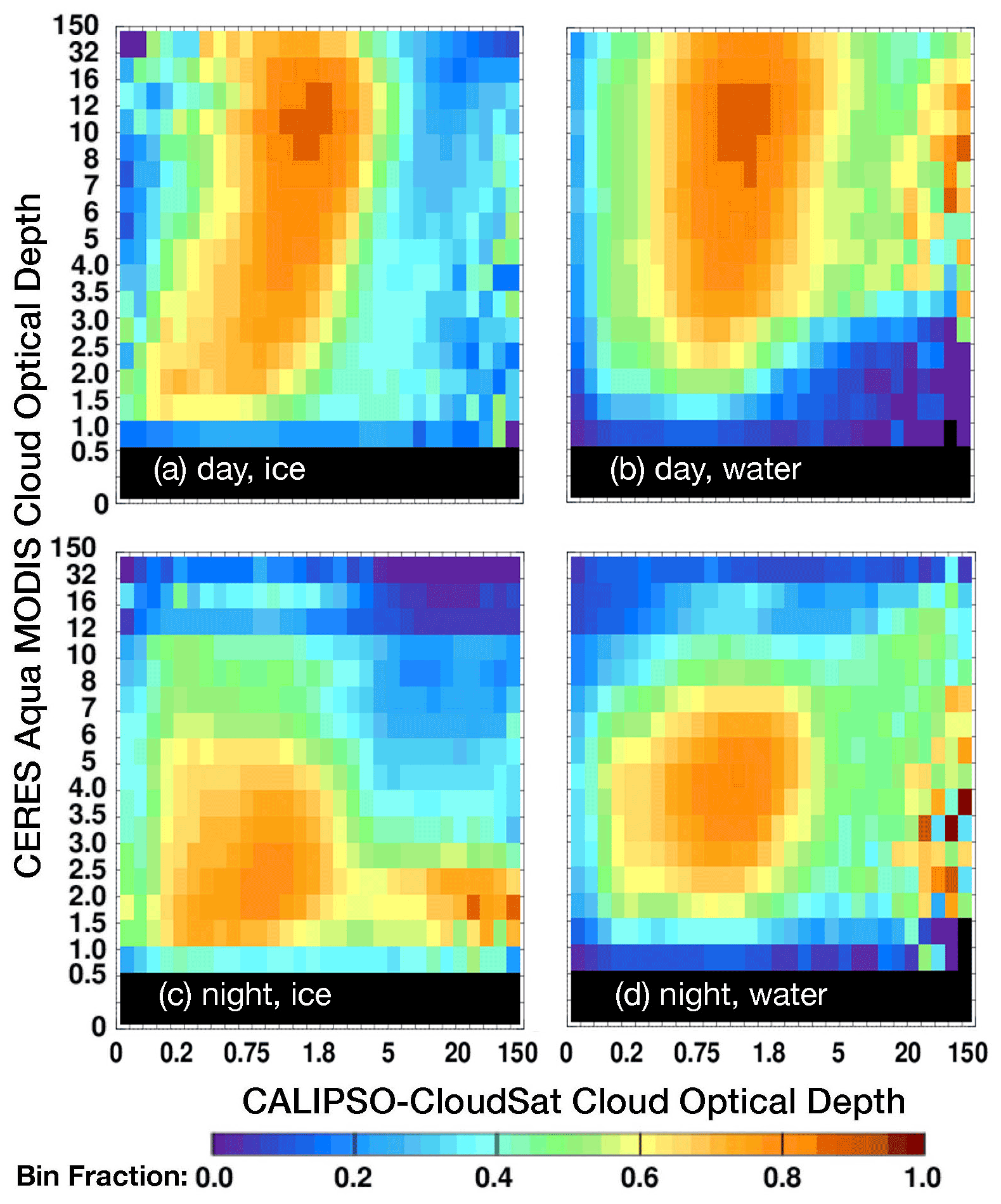
Figure 6 Recall or fraction of ML clouds detected within a given CC and CM cloud optical depth bin, 2009. Note the irregular axis scales. The tick marks for the x axis are 0, 0.0025, 0.05. 0.1, 0.15, 0.2, 0.3, 0.4, 0.5, 0.6, 0.75, 0.9, 1.1, 1.3, 1.5, 1.8, 2.1, 2.5, 3, 4, 5, 6, 8, 10, 15, 20, 30, 40, 60, 80, and 150.

At night, τ_CM is based only on thermal channels and, therefore, is mostly constrained to values of 8 or less. Default values of 8, 16, and 32 are employed whenever the cloud is assumed to be optically thick. The particular default value depends on the circumstances (Minnis et al., 2021). Sometimes, the CM4 and CM4+ analytical COD retrievals produce a value exceeding 8. Typically, τ_CM is closer to the upper-cloud COD at night, being influenced little by the lower cloud when the separation distance is large. Ignoring the high τ_CC bins, the nocturnal RC maxima are found around bins (1.1, 2.0) and (1.3, 4.5) for ice (Fig. 6c) and water clouds (Fig. 6d), respectively. True ML clouds are found more often than false SL clouds for 1 $<{\mathit{\tau }}_{\mathrm{CM}}<$ 5, when the phase is ice and 0.1 $<{\mathit{\tau }}_{\mathrm{CC}}<$ 3. The halfway COD bounds narrow to 0.2 $<{\mathit{\tau }}_{\mathrm{CC}}<$ 0.4 for greater values of τ_CM. For water-phase clouds, RC > 50 % occurs mostly for 1.5 $<{\mathit{\tau }}_{\mathrm{CM}}<$ 8 and 1.5 $<{\mathit{\tau }}_{\mathrm{CC}}<$ 4. It is clear that the thermal channel method is sensitive to thinner upper clouds compared to the daytime methods when the solar channel signal is overwhelmed by the lower cloud reflectances. Conversely, the daytime method detects more ML clouds when τ_CC> 3 or so.

This is more evident in Fig. 7, which shows histograms of the matrix parameters as a function of upper-layer τ_CC for MM and SM and τ_CM for SS and MS over SF surfaces. For water-phase clouds (Fig. 7a) the relative frequency of true ML pixels (MM), shown as solid lines, is greater at night than during the day when τ_CC< 0.5, but the occurrence of daytime MM pixels exceeds their nighttime counterparts when τ_CC> 0.9. Similar behavior is seen for the ice phase pixels (Fig. 7b), but the thresholds shift from 0.5 to 1.4 and from 0.9 to 1.9. The false SL or missed ML clouds (SM), shown as dashed lines, vary differently. For the ice phase pixels (Fig. 7b), the MM pixel frequency rises with increasing τ_CC up to ∼ 8 % at τ_CC= 3.5 before decreasing to 5 %–7 %, then dropping toward zero at τ_CC= 25. This peak for the thick ice clouds reflects the difficulty of inferring a lower layer under a nearly opaque cloud. For water-phase clouds (Fig. 7a), MM is most common for τ_CC< 0.3 and diminishes steadily to near zero around τ_CC= 30. As τ_CC increases, the ML system is more likely to be identified as ice phase, so fewer cases of ML systems having large upper-layer COD will be included in this population. In both cases, the night and day MM frequencies track each other relatively closely with τ_CC. Similar variations are found over the SC surfaces (not shown). Cumulative probability distribution functions based on the SF and SC results, presented in Fig. S1 in the Supplement, show that 50 % of the missed ML clouds have τ_CC< 0.25 for SF water clouds and < 0.5 for SC water clouds.

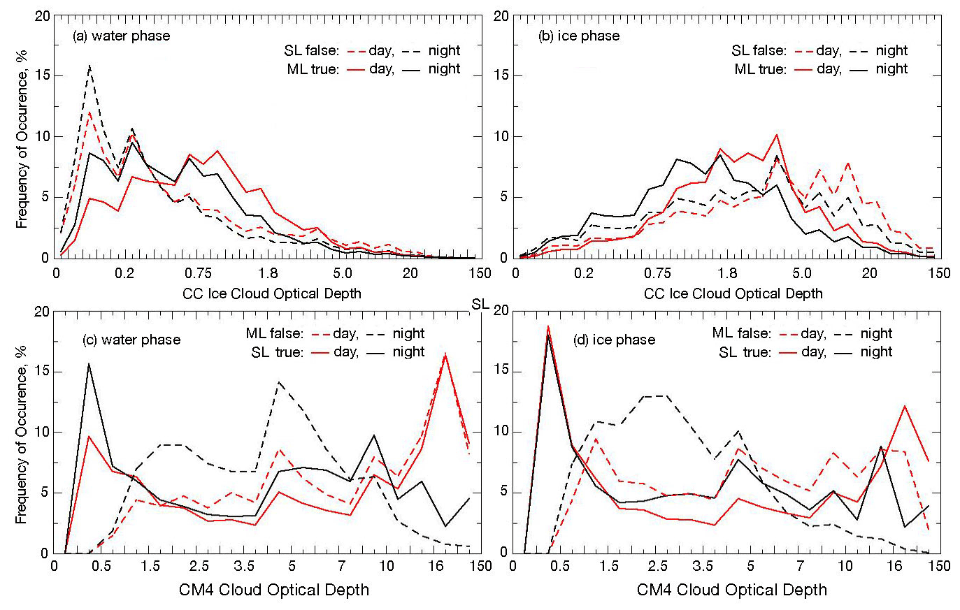
Figure 7 Probability distributions of 2009 false SL and true ML clouds from the MCANN as functions of upper-layer cloud optical depth over SF surfaces for Aqua MODIS (a) water phase and (b) ice phase. Probability distributions of 2009 false ML and true SL clouds from the MCANN as functions of total column cloud optical depth over SF surfaces for MODIS (c) water phase and (d) ice phase. The major tick marks for the x axes on the top panels are 0, 0.0025, 0.05. 0.1, 0.15, 0.2, 0.3, 0.4, 0.5, 0.6, 0.75, 0.9, 1.1, 1.3, 1.5, 1.8, 2.1, 2.5, 3, 4, 5, 6, 8, 10, 15, 20, 30, 40, 60, 80, and 150. The major tick marks for the x axes on the bottom panels are 0, 0.025, 0.5. 1.0, 1.5, 2.0, 2.5, 3.0, 3.5, 4, 5, 6, 7, 8, 10, 12, 16, 32, and 150.

Figure 7c and d show the frequency histograms of SS and MS for CC SL liquid and ice clouds, respectively, as a function of τ_CM. As expected, the peak SS (true SL) frequency occurs for τ_CM< 0.5 for both phases, day and night. During the day, a secondary true SL maximum is found around τ_CM≈ 25 for ice and water clouds. At night, that secondary peak is around τ_CM≈ 14 for ice pixels and near τ_CM≈ 9 for liquid clouds. Nocturnal false ML clouds (MS) are found mostly between CODs of 1 and 5 at night for ice pixels and between 2 and 6 for water clouds. During the day, MS occurs most often for τ_CM≈ 14 for water clouds. In fact, the MS frequency seems to follow the SS values, except for τ_CM< 0.5. The daytime MS occurrence is relatively flat for ice clouds with τ_CM> 1.0.

Another factor that can influence ML detection is the assumption that the lower cloud layer is composed of liquid water whenever the cloud temperature is less than 253 K. While that is true for most clouds, a small fraction of ice clouds have top temperatures (CTT) above 253 K (e.g., Hu et al., 2010). In those instances, the ML signal would likely be reduced because of similarities in the optical properties of the two layers. Mixed-phase clouds, which often occur in the supercooled temperature range, would have a similar effect but to a smaller degree depending on the amount of ice in the cloud. On the other hand, supercooled clouds globally account for about half of the clouds having an infrared CTT between 243 and 253 K. If only snow and ice surfaces are considered, the range is 239 to 242 K (see Fig. 6 of Hu et al., 2010). Thus, some systems with cold (CTT < 233 K) ice clouds over supercooled liquid clouds with CTT < 253 K could be identified as SL ice by the definition used here. These complementary effects due to supercooled clouds could produce some confusion in the training of the MCANN, particularly in polar regions.

The CODs used in the training would not be the same as those determined using the standard CM4 algorithms employed for the 2009 retrievals because the CM4+ algorithms used a different ice crystal model and a new method for retrieving COD over snow. This change in COD retrieval apparently had minimal impact on the detection as the 2008 training and 2009 validation results are nearly identical.

5.2 Comparisons with other results

As noted earlier, multilayered cloud detection has been the subject of many different algorithmic studies, so it is important to better understand how the current approach compares to those other algorithms. Direct comparisons are not straightforward because each algorithm was developed with its own specific constraints and ML definitions. The CERES Ed4 ML algorithm (Minnis et al., 2021) was applied only when a cloud with pressure below 500 hPa was detected using a CO₂-absorption method (Chang et al., 2010). The MODIS science team algorithm (Wind et al., 2010) was applied to a 5 km cloud product and was only used when the MODIS optical depth exceeded 4. The latest version, MYD06 C6.1 (Platnick et al., 2017), adds the BTD₁₁₁₂ technique developed by Pavolonis and Heidinger (2004). Desmons et al. (2017) used data from the POLarization and Directionality of the Earth's Reflectances (POLDER) to detect ML clouds of all types, but only for τ> 5. Ice-over-water multilayered clouds were detected by Wang et al. (2019) during daytime using Suomi National Polar-orbiting Partnership (SNPP) Visible Infrared Imaging Radiometer Suite (VIIRS) data in a thresholding method. Tan et al. (2022) placed no restrictions on either τ or the number of layers, but they applied their random forest algorithm and other machine learning techniques only to geostationary Himawari-8 data. Because of its orbit, the Himawari-8 observations are taken over a full range of VZA when matched with the CC profiles, but the VZA is constant for a given location. Other published methods have either not produced extended datasets or performed only case-study evaluations with objective data. Despite the sampling disparities, it is informative to compare some of the statistics to provide some context to the performance of the MCANN. These comparisons are summarized in Table 5.

Table 5 Confusion matrix metrics in percent for various multilayer algorithms. MYD06 and POLDER 95 are based on Table 4 of Desmons et al. (2017). VIIRS results are from Wang et al. (2019). Himawari results are based on Tan et al. (2022) random forest results. MCANN results are based on the 2009 validation parameters in Table 4. The horizontal line among the data separates results for day (top) and night (bottom). Values in italics denote partially complete Himawari validation metrics.​​​​​​​

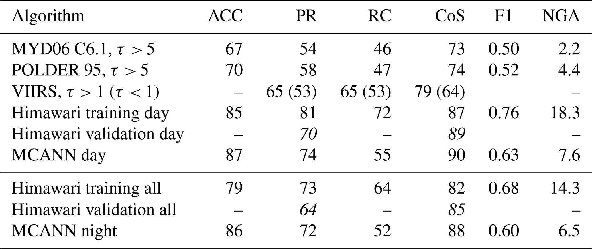
Comparing with CC data, Desmons et al. (2017) found that for overcast clouds with τ> 5, ACC = 70 % and CoS = 74 %. For the same conditions, they determined that MYD06 C6.1 yields ACC = 67 % and CoS = 73 %. Additional parameters computed from their Table 4 are listed in Table 5. Precision and recall from MYD06 are 54 % and 47 %, respectively, while they are 58 % and 47 % from POLDER. These can be compared to the MCANN daytime validation results (Table 5), which combine the SC and SF daytime data in Table 4 weighted by 0.13 and 0.87, fractions that roughly correspond to the areal coverage of the respective surface types (e.g., Yost et al., 2023). All of the MCANN parameter values exceed their restricted MYD06 and POLDER counterparts. Wang et al. (2019) only reported validation results in terms of percent of CALIOP ML and SL. Thus, only RC and CoS could be determined from their results. For τ> 1, the recall is about the same as the daytime MCANN value if the ML and probably ML categories from their algorithm are combined. Similarly, their CoS is ∼ 10 % smaller than the MCANN value. If clouds with τ< 1 are included, both CoS and RC drop substantially. Note that Wang et al. (2019) did not include CloudSat retrievals in their evaluation, so ML clouds with an optically thick upper cloud are not included in the statistics.

Although no value for ACC was given, the values of certain parameters can be estimated for all clouds with an unrestricted optical depth from the figures in Desmons et al. (2017). From their Fig. 8, RR ≈ 38 %, so ACC = 62 %. The value of CoS is the same for restricted and all clouds. The MODIS parameters change only negligibly for all clouds compared to the restricted case because the MYD06 algorithm only uses clouds with τ> 4. Marchant et al. (2020) also compared the MYD06 to the 2B-CLDCLASS-lidar products and found that for clouds with τ> 4, ACC = 63 % with the Pavolonis and Heidinger (2004) algorithm and 65 % without it. If it is assumed that all clouds with τ< 4 are SL clouds, then ACC jumps to 80 % and 81 % for the two algorithm options. But that assumption excludes 45 % of the ML clouds as defined by Marchant et al. (2020).

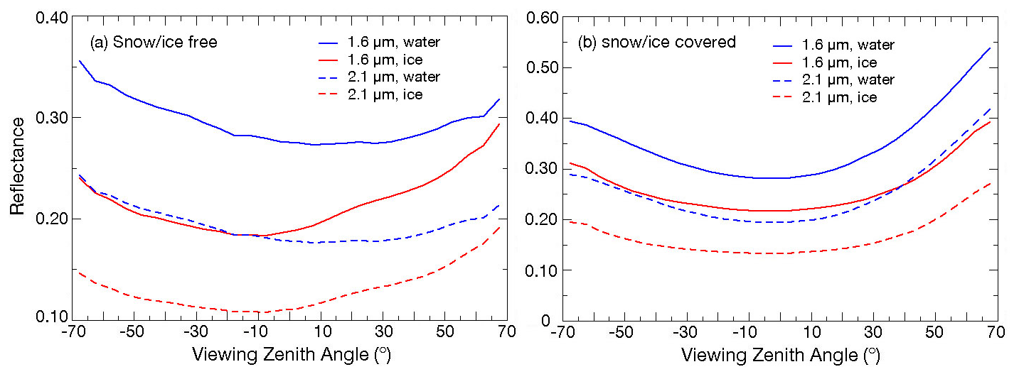
Figure 8 Mean reflectance from Aqua MODIS as a function of VZA for CERES water and ice-phase clouds, JAJO 2019.

Except for the definition of what constitutes a ML cloud (ice over water, water over water, etc.), NGA is the one parameter that is not too dependent on cloud optical depth assumptions. From Desmons et al. (2017), the daytime POLDER and MYD06 C6.1 cases yield NGA = 4.4 % and 2.2 %, respectively. Presumably, some of the POLDER results include water-over-water clouds. Nevertheless, the POLDER algorithm yields a net gain in information. The results of the Marchant et al. (2020) analysis yield slightly lower numbers for the MODIS C6.1 NGA, 0.2 % and 1.4 %, with and without the Pavolonis and Heidinger (2004) method. In either case, the MCANN daytime NGA exceeds those of the MYD06 and POLDER techniques. Moreover, it greatly exceeds the CERES Ed4 ML results (not shown). The F1 scores track the relative NGA rankings with the Himawari training values at the top followed by the MCANN, POLDER, and MODIS C6.1 in diminishing order.

The random forest results from Tan et al. (2022), confined to 60° S–60° N and 80° E–160° W, were trained with 1 km matched 2B-CLDCLASS-lidar profiles using the product's layer flag to determine if a given pixel is SL or has more than one layer, regardless of layer phase. That training dataset produced ACC = 85 % and 79 %, respectively, for the daytime and all-hour algorithms. The latter method included no reflectance input from solar channels, so it can be used for both day and night conditions. It is included in the bottom section of Table 5 for comparison to the MCANN night version. For this technique, PR = 81 % and 73 % for day and all-hours, respectively, with corresponding RC values of 72 % and 64 %. While ACC is less than that found with the MCANN for both day and night, the random forest PR and RC results are greater than their MCANN counterparts. At night, the MCANN PR is nearly equal to the Himawari-All value. The Himawari CoS and NGA daytime values were deduced from the values in their Table V and their Eqs. (1)–(3). The MCANN CoS values exceed their Himawari counterparts, but the MCANN global NGAs are less than half of those from the random forest training results. Those larger values arise, in part, from including many more types of ML clouds in the random forest training than used for the MCANN.

A fairer comparison would use independent validation sets from both algorithms. While a complete summary of the validation comparisons was not provided in Tan et al. (2022), several parameters can be determined from their Fig. 5, which utilized a dataset independent of the training data. The resulting values of PR are 70 % and 64 % for day and all-hours, respectively, while CoS = 89 % and 85 %. The MCANN SL confidences are slightly greater at 90 % and 88 % and its PR values exceed the Himawari validation results, especially for night/all-hours. Without further information it is not possible to determine the values of ACC and RC for the geostationary validation dataset. However, because CoS is the same or larger for the validation dataset and PR dropped by 11 points from the training results, it can be inferred that the fraction of false ML clouds increased considerably. This would reduce ACC and substantially diminish NGA.

Interestingly, the best results from the Tan et al. (2022) validation analysis are for ice-over-liquid and ice-over-mixed clouds. The former corresponds to conditions that the MCANN was developed to detect, while at least some of the latter were included in the MCANN analysis. Approximately 30 % of the actual ML clouds detected in the Tan et al. (2022) validation analysis are for single phase or upper-layer mixed phase ML clouds that MCANN was not designed to identify. Assuming that the portion of the ice-over-water/mixed is the same for the training dataset, the correctly detected ice-over-water cloud amount is 0.10. Adding the ice-over-mixed would yield 0.17. Reducing that by the ratio of PRs from the validation and training sets would drop the range to 0.09–0.15, which bounds the correct ML fraction from the SF cases in Table 4.

5.3 Full-swath detection

The MCANN training is based on near-nadir measurements from both the CC and MODIS instruments. Increasing optical path lengths due to increasing VZA modify the radiances emanating from a given location through absorption and scattering. This is particularly true for radiances at solar wavelengths. Thus, the near-nadir-based MCANN coefficients are not necessarily valid for observations taken at other VZAs. For operational use with Aqua MODIS data, the MCANN must be reliable across all viewing angles.

5.3.1 Angular dependence

The VZA dependency is examined by first computing the mean radiances for each viewing angle across the full scan for data taken during JAJO 2019. It was found that the radiance VZA dependence is sensitive to the forward or backward portion of the scan cycle. The former view is toward the Sun, while the latter is directed away from the Sun. Figure 8 plots the reflectance averages for each VZA bin in the forward (positive) and backward (negative) directions. From near-nadir to 65°, the 1.60 µm reflectance (solid lines) for water-cloud pixels increases by 11 % and 25 % in forward and backward directions, respectively. For ice clouds, the corresponding increases are 22 % and 37 %. Similar changes are seen for the 2.13 µm reflectances (dashed lines). The 1.38 µm reflectance for ice behaves in much the same manner (Fig. S2) but is nearly constant with VZA for water clouds. The daytime 3.75 µm radiances (Fig. S3) are relatively flat in the backward direction, but increase with VZA for liquid clouds. At night, the radiances show the classic limb-darkening behavior of thermal radiation. This can be seen in Fig. 9. During the day (solid lines), the water-cloud 10.8 µm radiances are relatively flat in the forward direction and drop a little at the higher VZAs in the backward direction. Ice-cloud radiances decrease in both directions, but more so in the forward view where the 10.8 µm radiances are lower than their back-direction counterparts. The forward scan views more shadowed areas that could affect the thin-cloud and partly cloudy scenes over land (Minnis et al., 2004). At night (dashed lines), the limb-darkening is more apparent. No backward or forward differences are considered at night. Similar variations in radiance are seen at 8.55 µm (Fig. S5) and 11.90 µm (Fig. S6). There are only minor radiance differences between the forward and backward directions during the day for the 6.70 µm channel (Fig. S4), presumably because it is mostly unaffected by the layers below the cloud. Additional plots of radiances as a function of VZA (Figs. S6–S14) are provided in the Supplement.

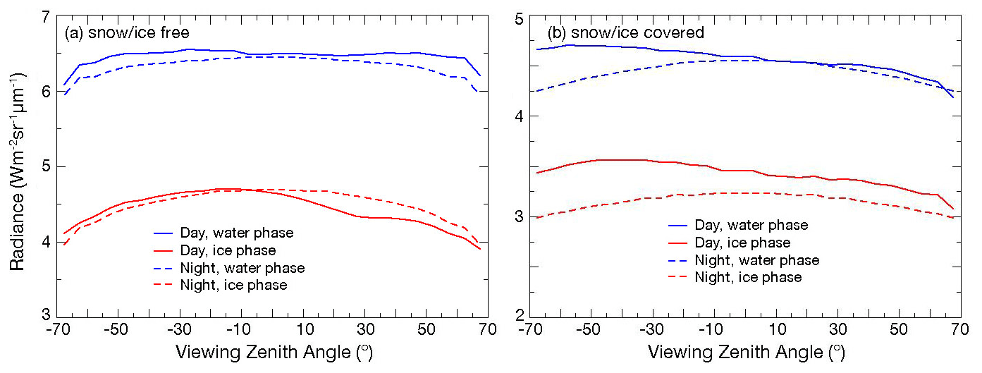
Figure 9 Mean 10.8 µm radiance from Aqua MODIS as a function of VZA for CERES water and ice-phase clouds, JAJO 2019.

To adjust the MODIS radiances, ice and water correction factors were determined for each waveband (day and night) separately over SF and SC surfaces. For daytime, the correction factors were computed for both forward and backward scans. These factors were developed for both the channel radiances and reflectances and each of the BTD parameters. The correction factor is simply the ratio of the mean radiance for VZA between −3 and −18° divided by the mean radiance at a given VZA. Thus, the observed radiance is adjusted to the near-nadir view of MODIS by simply multiplying it by the correction factor.

To test the impact of these factors on the retrievals, the MCANN was applied to the uncorrected and corrected full-swath MODIS data for April 2009. Figure 10 shows the variation of mean ML fraction as a function of VZA for SF ice and water clouds, day and night. During the day (Fig. 10a), the uncorrected and corrected ML fractions are nearly identical, suggesting that the correction factors for water-phase clouds have minimal effect on the radiances. This is not surprising, given the relatively flat daytime curves in Fig. 9 and for other thermal channels. In contrast to the daytime results, the nocturnal ML fractions have a nonmonotonic variation with VZA for the uncorrected radiances and a significant steady decrease to a value near zero for the corrected case. The uncorrected radiances for daytime ice clouds (Fig. 10b) yield a rise in ML detection in the forward direction with a much smaller rise in the backward direction. At night, the ice-cloud ML amounts drop for $\left|\text{VZA}\right|>$ 40°. When the correction factors are applied to the radiances, the ML amounts are relatively constant with VZA for both time periods. To obtain the most consistent product across the swath, the adjustments are applied to all of the radiances, except for water-cloud pixels observed during the night.

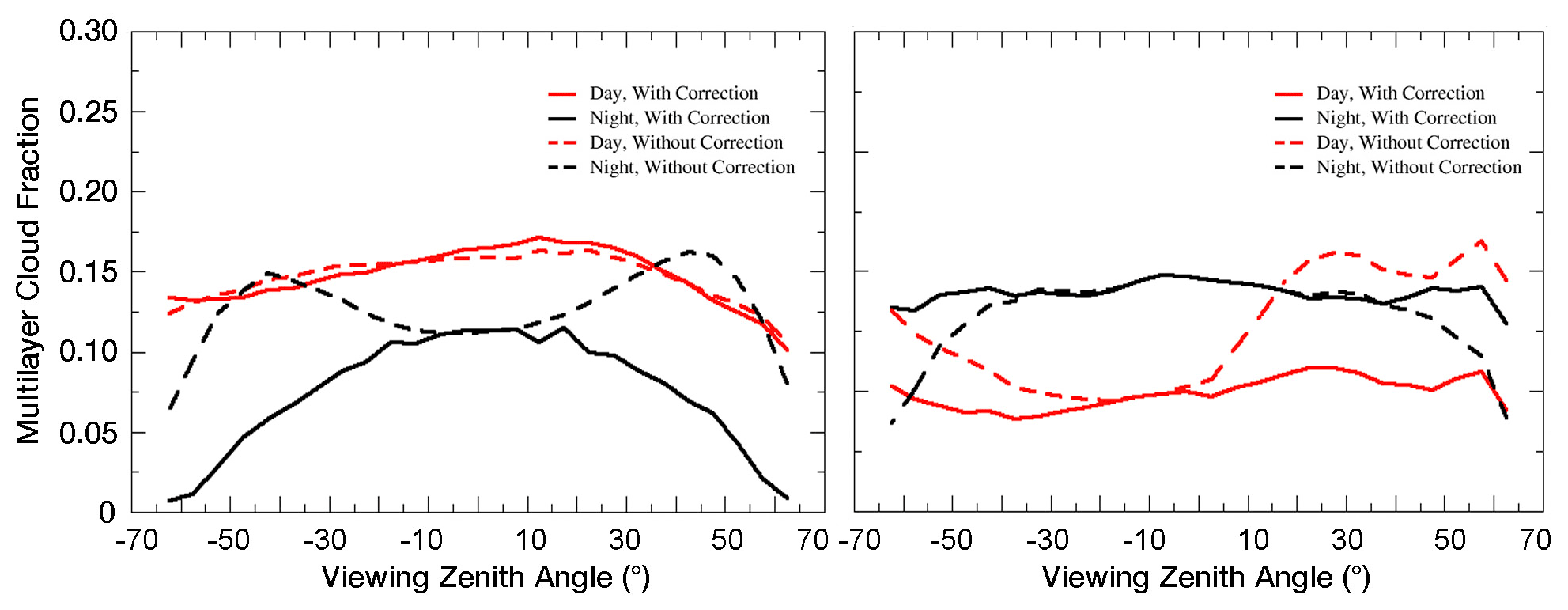
Figure 10 Mean MCANN multilayer cloud fraction from Aqua MODIS as a function of viewing zenith angle, April 2009. The MCANN was run with the MODIS data as observed (“Without Correction”) and after applying a VZA correction (“With Correction”).

5.3.2 Example images

Figure 11 shows the results of applying the MCANN with VZA correction to an Aqua MODIS image taken over the Southern Ocean centered near 57° S, 165° E at ∼ 03:50 UTC, 16 April 2019. The pseudo-color RGB image (Fig. 11b) shows an extensive area of stratocumulus on the left side that is apparently overlaid with thin cirrus that blurs the view of the underlying clouds. A second extensive liquid cloud deck appears near the top center that might overlay some stratocumulus clouds but is itself covered by thicker ice clouds. The CM4 cloud phase results (Fig. 11a) highlight those contiguous dense ice clouds, which likely obscure lower clouds. Thin cirrus also appear to overlie parts of the second liquid deck. The MCANN (Fig. 11c) determines that a large portion of the image consists of ice-over-water clouds. In general, the outline of the cloud effective heights (CEHs) above 1 km correspond to the ML pixels (Fig. 11d) except where the ice cloud is very thick, or perhaps, the ice cloud is in close proximity to or contiguous with the lower deck, as over parts of the white clouds in the top center part of the image. Other higher, SL liquid clouds are seen near the top left corner and bottom right of center. Cloud phase is very mixed over the thin cirrus areas, yet the MCANN determines most of the pixels as ML.

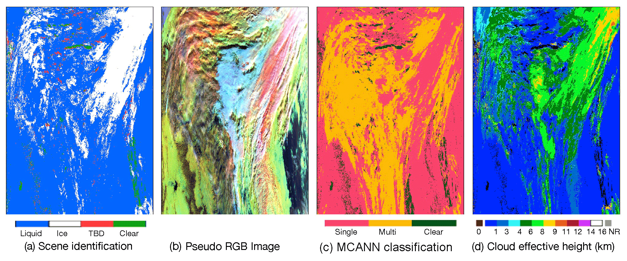
Figure 11 Cloud parameters derived from Aqua MODIS data between 62° S (top) and 52° S (bottom) around 165° E, at ∼ 3:50 UTC, 16 April 2019. (a) CM4 pixel scene classification, (b) pseudo-color RGB image (red: 0.64 µm reflectance, green: BT₃₇, blue: reverse BT₁₁), (c) the MCANN classification, and (d) the CM4 cloud effective height.

Multilayered clouds detected with the nighttime MCANN are shown in Fig. 12 for a MODIS image taken around 04:45 UTC the same day over the North Atlantic. The scene (Fig. 12b) contains extensive but variable cirrus coverage (white) and broken stratus clouds typically between 1 and 3 km (Fig. 12d). Thicker cirrus clouds are identified as ice (Fig. 12a), while many of the faintest ones, primarily those over the low clouds, are classified as liquid. Denser ice clouds and those over open water appear to be at altitudes between 9 and 14 km, while the thin cirrus over stratus range from 3 to 7 km, which is expected, given the SL cirrus altitudes. The MCANN appears to identify many of those ML clouds (Fig. 12c) but tends to miss those with overlying thick cirrus. There may be some false ML clouds in the upper right, but it is difficult to tell because the thinnest cirrus is not always discernible in the RGB image.

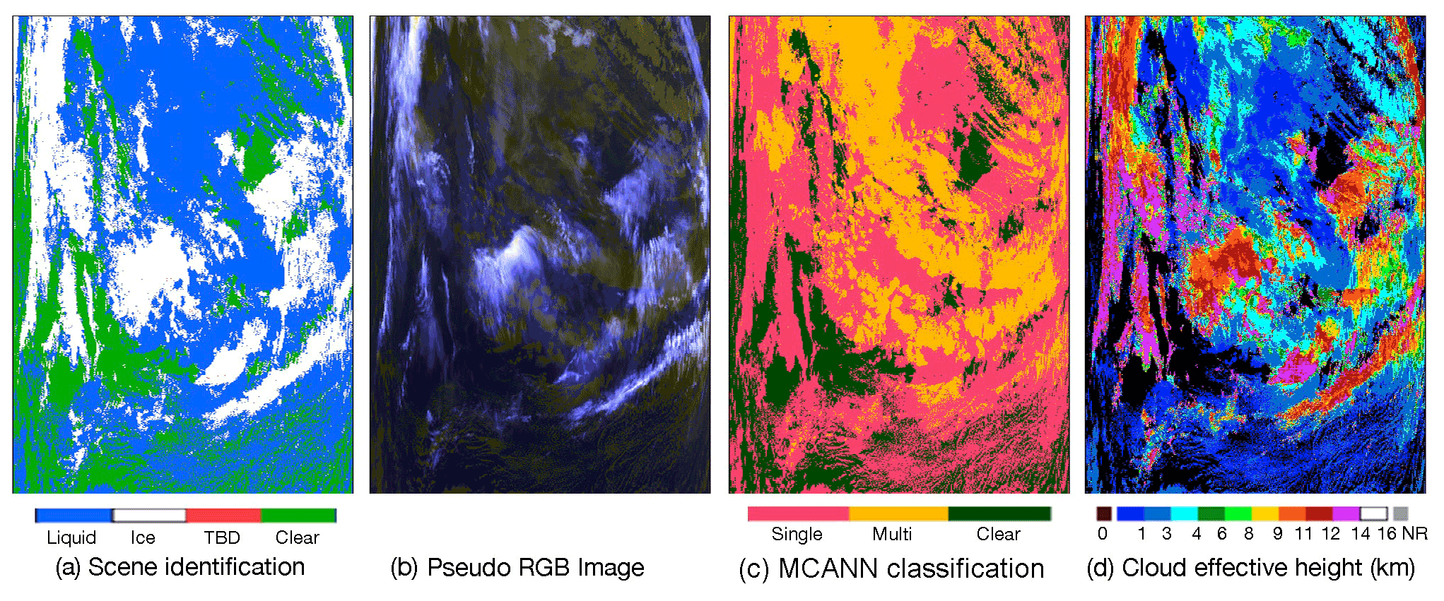
Figure 12 Cloud parameters derived from Aqua MODIS data between 42° N (top) and 24° N (bottom) around 50° W, at ∼ 04:45 UTC, 16 April 2019. (a) CM4 pixel scene classification, (b) pseudo-color RGB image (red: reverse BT₁₁, green: reverse BT₁₂, blue: BTD₃₇₁₁), (c) the MCANN classification, and (d) the CM4 cloud effective height.

The final example shown here (Fig. 13) is taken the same day around 01:50 UTC over the polar ice cap centered near 80° N, 155° E. Snow cover and ice cover provide the scarlet background (Fig. 13b), which is overlaid with low clouds in various shades of white to gray and a slightly higher deck in the center with thin cirrus covering much of the top half of the image. That cirrus appears as blurry pinkish gray and identified as ice or liquid depending on the thickness (Fig. 13a), while most of the cirrus over the deck in the middle is designated as liquid. Those clouds are identified as ML by the MCANN along with the small area at the bottom and in the upper left (Fig. 13c). Only a few parts of the cloud left of center are classified as ML, while it appears more ML clouds should have been detected. Most of the SL ice-cloud CEHs are only between 3 and 6 km (Fig. 13d), while those over the middle deck are less than 3 km. The low CEH values are likely due to overestimation of the COD by the CM4 retrieval for SL clouds and to the presence of the thick lower cloud for the ML retrievals. Detection of the ML clouds will allow for reclassification of the cloud tops as ice and recalculation of the cloud properties, when the components of a two-layer retrieval system are in place.

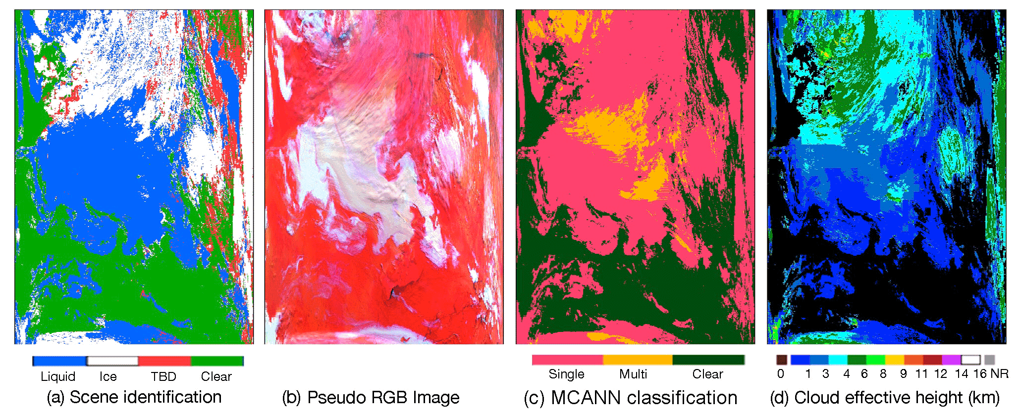
Figure 13 Cloud parameters derived from Aqua MODIS data between 77° N (top) and 83° N (bottom) around 155° E, at ∼ 01:50 UTC, 16 April 2019. (a) CM4 pixel scene classification, (b) pseudo-color RGB image (red: 0.64 µm reflectance, green: BT₃₇, blue: reverse BT₁₁), (c) the MCANN classification, and (d) the CM4 cloud effective height.

These three examples and the two additional cases shown in Figs. S15 and S16 demonstrate that the MCANN performs reasonably well across the full swath. No wild false ML clouds are evident although some recognizable misses are seen, as expected from the analyses above. Quantifying the accuracy of the correction-factor approach to full swath application of the MCANN would ultimately require using the method on similar data taken by a different satellite, such as SNPP VIIRS, that overlapped with the CC data at various VZAs. Using VIIRS data, Wang et al. (2019) found that the ML clouds they detected showed minimal changes with VZA. That result is similar to the daytime curves in Fig. 10b. Developing and analyzing a comparable VIIRS-CC dataset are beyond the scope of this paper, but they are planned for future research.

5.3.3 Assessment of full swath results

In the interim, more indirect approaches are available. For example, the off-nadir and near-nadir results should be spatially consistent if the swath approach is working properly. To examine this aspect, Fig. 14 shows the distributions of ML cloud fractions averaged over the months of January, April, July, and October (JAJO) 2009 from three different data sources. These include daytime retrievals from all CC data (Fig. 14a) and from the MCANN applied to Aqua MODIS radiances observed at the reference near-nadir (−3° < VZA < 18°) angles (Fig. 14b), and to Aqua MODIS data taken at all VZAs (Fig. 14c). The corresponding nocturnal results are plotted in Fig. 14d–f. These results are noisier than those in Fig. 3 because they are based on only 4 months of data and they include all observations, not just those having good CC and C3M cloudy pixel matches. The MODIS results include both false and partially cloudy pixels.

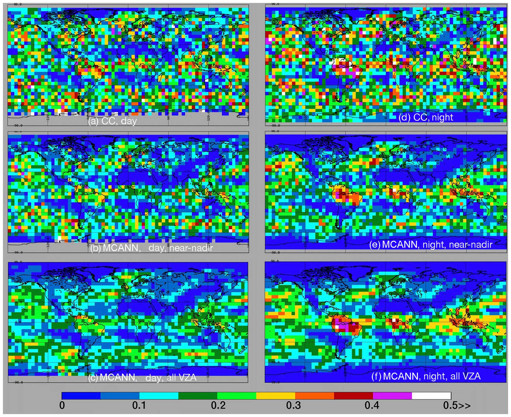
Figure 14 Multilayer fraction of total cloud cover for JAJO 2009 using all CC data from 2009 (a, d), and using Aqua MODIS MCANN retrievals (b, e) at near-nadir (−18° < VZA < 3°) and (c, f) for all VZAs; daytime on left, nighttime on right.

As in Fig. 3, the CC and near-nadir patterns are comparable, although the MCANN means are often smaller than their CC counterparts. The areas with minimal ML amount in the near-nadir results (Fig. 14b) are in the same locations as those from the CC retrievals, but they are more pronounced. Some CC maxima are reproduced by the MCANN, but the MCANN fractions near the maxima drop off more precipitously than their CC counterparts. For example, the maximum off the southern Chilean coast in Fig. 14b is nearly identical to that in Fig. 14a, but the MCANN fractions in the surrounding areas are generally smaller than the CC values. While much smoother, the nonpolar patterns in both all-VZA cases (Fig. 14c) are similar to those from the near-nadir results, but the Chilean maximum is diminished somewhat. Linear regression between the daytime CC and the MCANN regional means yields R² values of 0.80 and 0.66 for the near-nadir and full-swath results, respectively. The smaller value for the full-swath data is not surprising given its greater sampling. For the matched near-nadir and full-swath means, R²= 0.81.

Distributions of ML fractions from the same datasets appear to be more consistent at night. The maxima over northern South America, central Africa, and Indonesia are well defined in all three maps. Like the daytime results, the nonpolar minima are much better delineated in Fig. 14e and f than in the CC data (Fig. 14d). The correlation coefficients are 0.71 and 0.64 for the nocturnal CC regional means matched with their respective MCANN near-nadir and full-swath counterparts, while R² is 0.89 for the matched near-nadir and full-swath averages. Overall, the distributions in Fig. 14 demonstrate that the full-swath MCANN does not yield spurious ML clouds in areas where they are not expected to occur and generally produce results similar to the near-nadir values.

Another measure of robustness of the algorithm is its ability to reproduce the seasonal cycle. This is examined by computing the monthly mean ML anomaly, which is defined as the monthly mean minus the annual average divided by the annual average. It is clear that the SC results over snow miss many ML clouds, especially at night. Thus, to minimize the influence of SC regions on the seasonal cycle, only nonpolar (60° S–60° N) data are considered. Figure 15 plots the ML fraction anomaly for each month of 2009 from CC and the MCANN applied to full-swath Aqua MODIS data. The MCANN day and night anomalies track their CC counterparts remarkably well, within a few percent in most cases. The values of R² between the CC and MCANN monthly means are 0.92 and 0.90 for day and night, respectively.

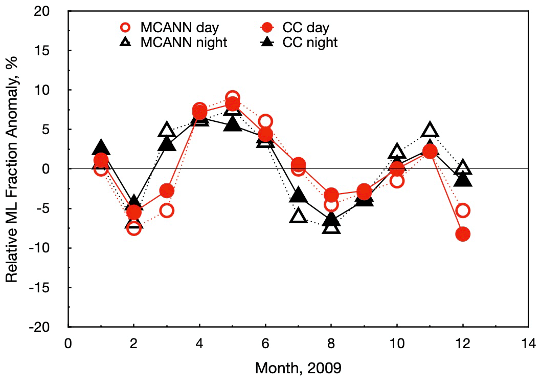
Figure 15 Monthly mean anomaly of multilayer fraction relative to total cloud cover for 2009 using all CC data and full-swath Aqua MODIS data.

To further examine the reliability of the MCANN on longer timescales, it was applied to January, April, July, and October (JAJO) 2013 Aqua MODIS full-swath data. The global distributions of the 2009 and 2013 results (Fig. S16) are similar but reveal shifts in the locations of the maxima. Table 6 presents the global mean JAJO 2009 and 2013 ML fractions along with the land–ocean ratio, L $/$ O, which is the global average ML fraction over land divided by that over water surfaces. Overall, ML fractions for all CC data are 3 %–5 % greater than their MODIS-matched counterparts, a result comparable to the differences in Fig. 4. The 2009 MCANN near-nadir values are 0.01 smaller than those for all VZAs. ML fractions in Table 6 are all less than their counterparts in Fig. 4. This is due to the fact that the CC data in Table 6 include all cloudy pixels that the CERES cloud mask classified as clear, and the MCANN results include many partly cloudy pixels that are not likely to be ML. The clouds detected by CALIPSO, but missed by CERES, are mostly SL thin cirrus and SL low clouds (Yost et al., 2021, 2023), which would dilute the ML fraction determined using all of the CC data. The differences between the CC and near-nadir MCANN are reduced by ∼ 2 % compared to those using only the matched data. During daytime, the MCANN mean ML fractions from 2013 are 0.5 % greater than those in 2009, while at night the 2013 averages exceed their 2009 counterparts by 0.2 % near nadir and 0.6 % across the full swath. For both years, the nocturnal near-nadir values are ∼ 1 % less than for data taken at all VZAs.

Table 6 Average ML fractions from CC and Aqua MODIS MCANN for JAJO.

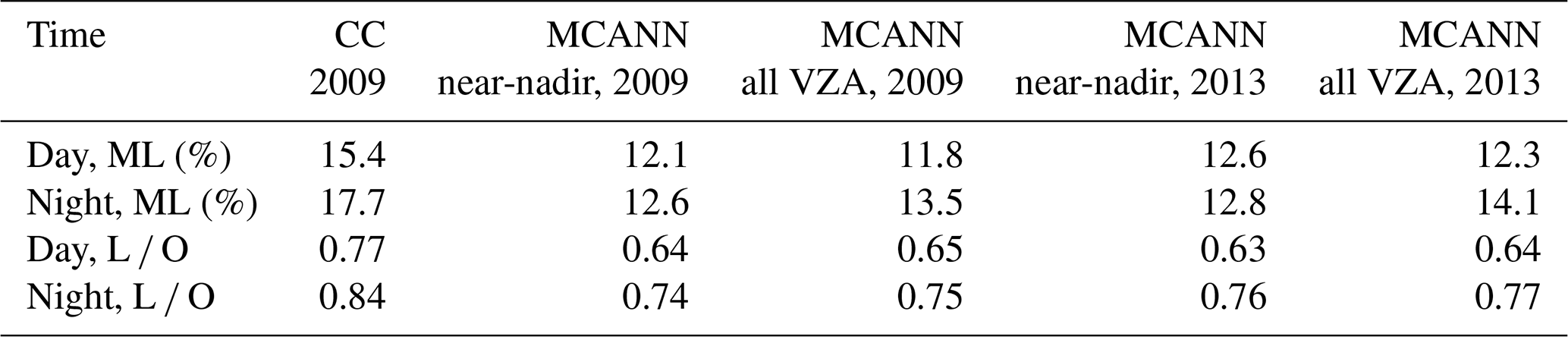
The CC land–ocean ratios, L $/$ O, in Table 6 reveal that fewer ML clouds occur over land than over water surfaces. For CC, L $/$ O is between 0.77 and 0.84, while it varies from 0.64 to 0.77 for the MCANN results, indicating that the MCANN is less efficient at detecting ML clouds over land than over water bodies. Together with the similarity of the CC and ML seasonal cycles, the consistency of the near-nadir and full-swath L $/$ O values and small differences in ML amounts during both years are quite encouraging for using the MCANN on an operational basis.

5.3.4 Operational considerations

CERES is a long-term project that utilizes many different satellites and imagers to characterize cloud properties. The MODIS imagers on Aqua and Terra and the VIIRS imagers on SNPP and NOAA-20 are coincident with the CERES broadband radiometers and observe nonpolar regions at fixed times each day. Any system designed to detect ML clouds should be applicable to both the VIIRS and MODIS imagers and, ideally, to the geostationary imagers that are used to help assess the radiation budget at other times of day. Because the latter have had widely varying spectral channel complements since 2000, use of the MCANN with them is beyond the scope of this discussion. The VIIRS lacks certain channels used here (13.3 and 6.7 µm), and the channels common to MODIS and VIIRS differ in spectral coverage and filtering. Additionally, the VIIRS is a higher-resolution instrument. Thus, it may be necessary to train VIIRS with CC data to obtain a consistent ML result. Another approach would require careful intercalibration of the VIIRS and MODIS channels using spectral corrections (e.g., Scarino et al., 2016) and the addition of radiances from the missing channels determined from a process that fuses data from VIIRS and the Cross-track Infrared Sounder (e.g., Weisz et al., 2017). If those are not available, then the MCANN would need to be retrained with fewer input radiances, likely at the expense of accuracy. To that end, initial training tests indicate that without those channels, ACC decreases from 87.0 % to 86.4 % during the day and from 85.6 % to 84.3 % during the night over SF surfaces. During the day, NGA drops from 7.6 % to 7.1 %, while at night NGA goes from 7.3 % to 6.2 %. NGA is relatively unaffected by the loss of the 13.3 µm channel; almost all of the diminished accuracy is due to the absence of the 6.7 µm channel, particularly at night. Even with the loss of those channels, the resulting detection capability would still represent a significant advancement over previous efforts.

As in all retrievals, reliable and consistent calibration across platforms is essential to providing an accurate ML product. It may be even more important for the MCANN, because the neural network relies on subtle radiance differences that may be lost in the noise of a physical retrieval. Thus, any small trend in the calibration of one channel may introduce a growing bias in the ML fraction. Similarly, inter-platform calibration differences could cause a similar effect. Updated retrieval algorithms and input data are introduced into the CERES data processing whenever major improvements are developed and errors diminished. Since the MCANN relies on a few retrieval inputs such as COD and cloud phase, it would need to be retrained whenever a new CERES cloud algorithm edition is introduced.

Further improvement of the MCANN itself, particularly over snow-covered areas, might be gained by using additional parameters or spatial context. For example, Tan et al. (2022) found that radiances from the 7.3 µm channel comprise a highly ranked predictor of ML clouds in their random forest approach. The MODIS equivalent channel was not considered here but would have to be created for VIIRS using the fusion process noted above. Information about the pixels surrounding the pixel of interest increased the accuracy of ice water path retrieved from a Meteosat imager with a convolutional neural network (Amell et al., 2022). Including selected radiances or BTDs from surrounding pixels might also enhance the MCANN. Additional partitioning of the training categories might also raise ML detectability as it did when the original MLANN (Sun-Mack et al., 2017) was divided into ice and water phase categories (Minnis et al., 2019). These and other approaches could lead to greater accuracies than found here.

6 Summary and conclusions

An artificial neural network method has been enhanced to more accurately identify ice-over-water ML cloud systems from multispectral MODIS observations. The algorithm requires as input a variety of radiances, brightness temperature differences, atmospheric profiles of temperature and humidity, and the CERES Edition 4 cloud phase and optical depths. Based on the definitions of single and multilayer clouds used here for CALIPSO-CloudSat profiles, the MCANN correctly identifies SL and ML clouds together 87.0 % and 85.6 % of the time over surfaces free of ice and snow during day and night, respectively. Over ice or snow-covered areas, the corresponding correct identifications are 89.3 % and 88.7 %. Despite the good overall agreement, the MCANN only detects 55 % of the CC ML clouds over SF regions and only 40 % and 20 % over SC areas during day and night, respectively. The majority of the missed SF ML clouds are those having an upper-cloud COD < 0.3 (water) or COD ≥ 3 (ice), although ∼ 35 % and 20 % of the water and ice-phase detected ML clouds meet those conditions. Over SC surfaces, the undetected ML pixels mainly have an upper-cloud COD < 0.5 or COD > 2.

Direct comparisons of the MCANN to other multilayer cloud detection methods are not possible due to differences in ML cloud definitions, input satellite data, reported accuracy parameters, sampling, and cloud optical depth constraints. Nevertheless, the MCANN results were evaluated here against published results based on other techniques. Attempts were made to minimize the characteristic differences among the various results as much as possible. All conclusions drawn from those comparisons are limited by the unknown effects of the remaining differences among the methods.

Despite its shortcomings, the MCANN, unlike many other techniques, yields a significant net gain in layering identification accuracy because the number of false ML pixels is substantially less than that for true ML pixels. Overall, the daytime MCANN evaluation metrics are more favorable than those based on physical retrievals or decision tree algorithms. Few methods have been developed for nocturnal application. Comparisons with results from a machine learning algorithm applied to geostationary satellite data yielded a more ambiguous assessment. The accuracy and SL confidence from the MCANN are greater than those from the Tan et al. (2022) random forest training results for day and night. Yet, the MCANN precision, recall, and NGA values are smaller. If the validation results from Tan et al. (2022) are considered, the MCANN precision values are greater. It is not known how much the MCANN recall and NGA would fare relative to the random forest validation results. Even if it were known, the relative merits of the two methods would be difficult to quantify without accounting for the discrepancies in ML definition and sampling areas and time periods. However, it is concluded from the comparisons that the MCANN is among the most capable of current ML detection methods.

Operationally, the MCANN, trained with near-nadir MODIS views, must be applicable to all the MODIS viewing angles. To account for the variation of radiances with viewing zenith angle, the MODIS-based input parameters are normalized to the nadir view using empirical correction factors. The adjustments yield ML cloud amounts that are mostly invariant with VZA and produce visually reasonable ML detection across the MODIS swath. Spatial distributions of ML cloud fractions from full-swath results are consistent with the near-nadir results and manifest similar detection efficiencies over land and water surfaces that are the same as their near-nadir counterparts. Temporally, the MCANN produces the same seasonal cycle in ML clouds as the active sensor data, albeit with the noted bias. Moreover, the results are similar in magnitude and distribution for different years with shifts in maxima. While more detailed pixel-to-pixel comparisons should be performed using CC data matched to imagery taken at off-nadir VZAs, the analyses performed here indicate that the MCANN should be as successful off of nadir as it is in the near-nadir mode.

Applying the MCANN to other imagers should be performed with caution as sensors on other satellites can differ spectrally and spatially (e.g., VIIRS) or may observe at other times of day (e.g., Terra MODIS). Platforms that are not in Sun-synchronous orbits, e.g., geostationary satellites, will observe a given scene at times of day and at viewing and illumination angles that are not seen by Aqua MODIS and hence not in the training complement. Adapting the MCANN to different types of orbits or times of day presents a challenge as there are few options for global training and validation. Current and future cloud radar and lidar combinations are confined to afternoon Sun-synchronous satellites (e.g., Cerdeña et al., 2017). Lidars that can be used for cloud detection have flown on the International Space Station (e.g., Pauly et al., 2019) in a precessing orbit and on Aeolus in a sunrise/sunset Sun-synchronous orbit (Straume et al., 2020). CALIPSO has been slowly moving away from its 13:30 LT orbit, covering several more hours of the day since 2018. Without the cloud radar, any and all of those lidars could be used to define ML clouds to some extent, depending on their penetration depths, and may be of value for training and validating ML clouds for geostationary imager data. Regardless of the particular satellite, the MCANN would need to be retrained or the spectral channels normalized to MODIS.

With layer detection accuracies below 90 %, there is clearly room for future improvement, especially over polar regions covered with snow and ice. Use of additional channels or subsets of the current training categories may add a few more points to the overall accuracy. Combining physical retrievals with the neural network may also be the means for detecting more ML pixels. The definition of ML clouds used here is rather restrictive in that it is nominally confined to ice-over-liquid water clouds. It is also somewhat ambiguous because 253 K serves as the threshold between ice and water clouds for the underlying cloud deck. In lieu of any better information to define the lower cloud phase, the threshold should be altered to account for variability of the 50th percentile ice phase in the supercooled temperature range. Other cloud combinations such as liquid over liquid could be included in the MCANN but they might reduce the accuracy and would probably be more resolvable if treated separately from the ice-over-water clouds.

Detecting multilayer clouds is a first step toward improving the characterizations of global vertical cloud structure using passive sensors. Once identified, the upper and lower layer cloud properties need to be estimated. A number of approaches have been suggested for estimating the top heights of the upper and lower clouds. These include physical retrievals (e.g., Chang et al., 2010) and machine learning (e.g., Minnis et al., 2019). Similarly cloud optical depth and particle effective size could be derived with a physical retrieval (e.g., Chang et al., 2010), a neural network (e.g., Cerdeña et al., 2007), or an optimal estimation method that requires the cloud heights (e.g., Sourdeval et al., 2016). Having a reliable detection method, like the MCANN that operates in both sunlit and nocturnal conditions, should serve as motivation for formulating a robust technique for unscrambling the upper and lower cloud layer properties in future research.