the Creative Commons Attribution 4.0 License.
the Creative Commons Attribution 4.0 License.
 | 10 Jun 2024
High Spectral Resolution Lidar – generation 2 (HSRL-2) retrievals of ocean surface wind speed: methodology and evaluation
Sanja Dmitrovic
Johnathan W. Hair
Brian L. Collister
Ewan Crosbie
Marta A. Fenn
Richard A. Ferrare
David B. Harper
Chris A. Hostetler
Yongxiang Hu
John A. Reagan
Claire E. Robinson
Shane T. Seaman
Taylor J. Shingler
Kenneth L. Thornhill
Holger Vömel
Xubin Zeng
Ocean surface wind speed (i.e., wind speed 10 m above sea level) is a critical parameter used by atmospheric models to estimate the state of the marine atmospheric boundary layer (MABL). Accurate surface wind speed measurements in diverse locations are required to improve characterization of MABL dynamics and assess how models simulate large-scale phenomena related to climate change and global weather patterns. To provide these measurements, this study introduces and evaluates a new surface wind speed data product from the NASA Langley Research Center nadir-viewing High Spectral Resolution Lidar – generation 2 (HSRL-2) using data collected as part of the NASA Aerosol Cloud meTeorology Interactions oVer the western ATlantic Experiment (ACTIVATE) mission. The HSRL-2 can directly measure vertically resolved aerosol backscatter and extinction profiles without additional constraints or assumptions, enabling the instrument to accurately derive atmospheric attenuation and directly determine surface reflectance (i.e., surface backscatter). Also, the high horizontal spatial resolution of the HSRL-2 retrievals (0.5 s or ∼ 75 m along track) allows the instrument to probe the fine-scale spatial variability in surface wind speeds over time along the flight track and over breaks in broken cloud fields. A rigorous evaluation of these retrievals is performed by comparing coincident HSRL-2 and National Center for Atmospheric Research (NCAR) Airborne Vertical Atmosphere Profiling System (AVAPS) dropsonde data, owing to the joint deployment of these two instruments on the ACTIVATE King Air aircraft. These comparisons show correlations of 0.89, slopes of 1.04 and 1.17, and y intercepts of −0.13 and −1.05 m s−1 for linear and bisector regressions, respectively, and the overall accuracy is calculated to be 0.15 ± 1.80 m s−1. It is also shown that the dropsonde surface wind speed data most closely follow the HSRL-2 distribution of wave slope variance using the distribution proposed by Hu et al. (2008) rather than the ones proposed by Cox and Munk (1954) and Wu (1990) for surface wind speeds below 7 m s−1, with this category comprising most of the ACTIVATE data set. The retrievals are then evaluated separately for surface wind speeds below 7 m s−1 and between 7 and 13.3 m s−1 and show that the HSRL-2 retrieves surface wind speeds with a bias of ∼ 0.5 m s−1 and an error of ∼ 1.5 m s−1, a finding not apparent in the cumulative comparisons. Also, it is shown that the HSRL-2 retrievals are more accurate in the summer (−0.18 ± 1.52 m s−1) than in the winter (0.63 ± 2.07 m s−1), but the HSRL-2 is still able to make numerous (N=236) accurate retrievals in the winter. Overall, this study highlights the abilities and assesses the performance of the HSRL-2 surface wind speed retrievals, and it is hoped that further evaluation of these retrievals will be performed using other airborne and satellite data sets.
- Article
(14231 KB) - Full-text XML
-
Supplement
(627 KB) - BibTeX
- EndNote


The layer between the ocean and free troposphere, known as the marine atmospheric boundary layer (MABL), hosts various processes such as the modulation of sensible and latent heat fluxes, the exchange of gases such as carbon dioxide, the evolution of clouds, and the transport of aerosol particles (Neukermans et al., 2018). Improved characterization of MABL dynamics is required to accurately simulate large-scale phenomena related to climate change and global weather patterns (Paiva et al., 2021). This characterization relies on a combination of global numerical weather prediction (NWP) models and real observations (Carvalho, 2019). One of the most influential parameters that drives these MABL processes is ocean surface wind speeds or wind speeds at 10 m above sea level (hereafter called surface wind speeds). Therefore, instruments such as lidar are used to provide accurate surface wind speed measurements in various geographical locations to improve estimations of the MABL state globally. For instance, satellite lidar systems that measure aerosol and cloud vertical distributions, such as the lidar on board the NASA Cloud–Aerosol Lidar and Infrared Pathfinder Observation (CALIPSO) satellite, also have the capability to provide horizontally resolved surface wind speed data. The underlying principle of lidar surface wind speed retrievals was first derived by Cox and Munk (1954), where bidirectional reflectance measurements of sea surface glint are used to establish a Gaussian relationship between surface wind speeds and the distribution of wind-driven wave slopes. To probe these surface wave slopes, lidar instruments emit laser pulses into the atmosphere and measure the reflectance (or backscatter) of those laser pulses from particles, molecules, and the ocean surface. The magnitude of the measured signal is then used to estimate the variance of the wave slope distribution (i.e., wave slope variance) and therefore surface wind speed. Note that reflectance and backscatter are used interchangeably throughout this paper.
Although many studies have expanded upon the original Cox–Munk relationship (e.g., Hu et al., 2008; Josset et al., 2008, 2010a; Kiliyanpilakkil and Meskhidze, 2011; Nair and Rajeev, 2014; Murphy and Hu, 2021; Sun et al., 2024), these parameterizations do not account for atmospheric attenuation by aerosols and therefore have difficulty in calibrating the measured ocean surface reflectance accurately. This presents a difficulty for elastic backscatter lidars like CALIPSO, for which the signal is typically calibrated high in the atmosphere where molecular backscatter dominates and aerosol backscatter is insignificant or can be accurately estimated. The problem lies in the transfer of this calibration to the ocean surface, which entails accounting for the attenuation of the transmitted and backscattered light by the intervening atmosphere between the calibration region and the ocean surface. If coincident aerosol optical depth (AOD) data are available (e.g., from MODIS in the case of CALIPSO detailed in Josset et al., 2008), then they may be used to estimate the intervening attenuation and transfer the calibration. However, such data from passive sensors including MODIS are only available during daytime, are typically not produced in the vicinity of clouds, and may have unacceptably high uncertainties for accurately accounting for aerosol attenuation. Estimation of the attenuation from the lidar data alone requires an assumption of the aerosol extinction-to-backscatter ratio (or “lidar ratio”), so errors in the assumed value can lead to an incorrect estimate of attenuation, especially when AOD is high. Because of this, the surface wind speed estimates in Hu et al. (2008) were limited to scenes with no clouds and negligible aerosol loading.
This study addresses retrieving surface wind speed directly from lidar without other assumptions or external constraints by employing the high-spectral-resolution lidar (HSRL) technique through the NASA Langley Research Center (LaRC) airborne High-Spectral-Resolution Lidar – Generation 2 (HSRL-2) instrument (Hair et al., 2008). The HSRL-2 can directly measure vertically resolved aerosol backscatter and extinction profiles without relying on an assumed lidar ratio or on other external aerosol constraints, enabling accurate estimates of the attenuation of the atmosphere. Therefore, the surface reflectance can be directly determined, providing a measure of the wave slope variance and thus surface wind speed. Note that the HSRL-2 operates at a nadir-viewing geometry, which is detailed more in Sect. 2.4. At nadir or near-nadir incidence angles, the surface contribution of the lidar surface backscatter signal is the largest and is therefore sensitive to changes in wind speed (Josset et al., 2008, 2010a, b), making it possible to introduce relatively simplified models of sea surface reflectance. However, Li et al. (2010) demonstrated that for higher-incidence-angle lidar systems (> 15°), the sensitivity of the lidar surface signal would rapidly decrease as these highly non-nadir incidences shift the signal towards a subsurface contribution rather than a surface one. A more recent lidar study based on the highly non-nadir (∼ 37°) Aeolus UV HSRL (Labzovskii et al., 2023) indirectly confirms this phenomenon by showing low agreement between passive remote sensing reflectivity and Aeolus surface reflectivity parameters over water surfaces such as oceans. For these reasons, an opportunity to retrieve ocean surface wind speeds using lidar ocean backscattering has been shown to be effective only for nadir or near-nadir lidar systems such as the HSRL-2.
This study details the HSRL-2 surface wind speed retrieval methodology and evaluates this surface wind speed product through comparison with measurements from National Center for Atmospheric Research (NCAR) Airborne Vertical Atmospheric Profiling System (AVAPS) dropsondes. This work leverages an extensive data set from the NASA Aerosol Cloud meTeorology Interactions oVer the western ATlantic Experiment (ACTIVATE) mission, the multiple scientific and technological objectives of which are described in Sect. 2.1 (Sorooshian et al., 2019). The mission consisted of six deployments between 2020 and 2022 and featured the joint deployment of the HSRL-2 and dropsonde launcher on one of its two aircraft to enable direct comparison between the two instrument data sets. The mission, dropsonde and HSRL-2 instrumentation, HSRL-2 algorithm, and the methods and results of evaluating the accuracy of the HSRL-2 surface wind speed data retrievals are all detailed in the following discussion.
2.1 ACTIVATE mission description
The HSRL-2 ocean surface wind speed product is assessed during the ACTIVATE campaign, which is a NASA Earth Venture Suborbital-3 (EVS-3) mission. The primary aim of ACTIVATE is to improve knowledge of aerosol–cloud–meteorology interactions, which are linked to the highest uncertainty among components contributing to total anthropogenic radiative forcing (Bellouin et al., 2020). There are three major scientific objectives: (i) characterize interrelationships between aerosol particle number concentration (Na), cloud condensation nuclei (CCN) concentration, and cloud drop number concentration (Nd), with the goal of decreasing uncertainty in model parameterizations of droplet activation; (ii) advance process-level knowledge and simulation of cloud microphysical and macrophysical properties, including the coupling of aerosol effects on clouds and cloud effects on aerosol particles; and (iii) assess remote sensing capabilities to retrieve geophysical variables related to aerosol–cloud interactions. This study focuses on the third objective, which has already received attention with ACTIVATE data for retrievals other than ocean surface wind speeds (Schlosser et al., 2022; Van Diedenhoven et al., 2022; Chemyakin et al., 2023; Ferrare et al., 2023). ACTIVATE built a large volume of flight data statistics over the western North Atlantic Ocean (WNAO) by flying six deployments across 3 years (2020–2022), with a winter and summer deployment each year (Sorooshian et al., 2023). Winter deployments included the following date ranges: 14 February–12 March (2020), 27 January–2 April (2021), and 30 November 2021–29 March (2022). Summer deployments were as follows: 13 August–30 September (2020), 13 May–30 June (2021), and 3 May–18 June (2022). Across all 3 years, 90 King Air flights during the winter deployments were performed with 373 dropsondes launched, while 78 flights during the summer deployments took place with 412 dropsondes launched.
Two NASA Langley aircraft flew in spatial and temporal coordination for the majority of the total flights (162 of 179). A “stacked” flight strategy was developed where a low-flying (< 5 km) HU-25 aircraft collected in situ data in and just above the MABL, while a high-flying (∼ 9 km) King Air aircraft simultaneously provided remote sensing retrievals and dropsonde measurements in the same altitude range. In doing so, the stacked aircraft would simultaneously obtain data relevant to aerosol–cloud–meteorology interactions in the same column of the atmosphere and provide a complete picture of the lower troposphere (Sorooshian et al., 2019). In situ measurements of gases, particles, meteorological variables, and cloud properties were conducted by the HU-25 Falcon. The King Air payload included the NASA Goddard Institute for Space Studies (GISS) Research Scanning Polarimeter (RSP) and the two instruments relevant to this work: the NASA LaRC HSRL-2 and the NCAR AVAPS dropsondes (Sorooshian et al., 2023). An advantage of the joint deployment of HSRL-2 and AVAPS dropsondes on the King Air is that the data are spatially synchronized at launch, with wind drift of the dropsondes during descent accounted for with procedures summarized in Sect. 2.2.
The rationale for flying over the WNAO in different seasons was to collect data across a wide range of aerosol and meteorological regimes, with the latter promoting a broad range of cloud conditions (Painemal et al., 2021). A significant meteorological feature is the North Atlantic Oscillation, which is the oscillation between the Bermuda–Azores High (high pressure system) and the Icelandic Low (low pressure system; Lamb and Peppler, 1987). In the summer, the Bermuda–Azores High is at its peak and introduces easterly and southwesterly trade winds (Sorooshian et al., 2020). Starting in the fall, the Icelandic Low becomes prominent and introduces westerly winds in the boundary layer. The balancing act between these pressure systems dictates the climate of the North Atlantic and the prevailing transport processes (Li et al., 2002; Creilson et al., 2003; Christoudias et al., 2012). These transport processes that vary seasonally explain why winter flights coincided with more offshore (westerly) flow containing aerosol types impacted by anthropogenic influence (e.g., Corral et al., 2022), whereas summer flights included more influence from wildfire emissions and African dust, among other sources both natural and anthropogenic in nature (Mardi et al., 2021; Aldhaif et al., 2020). Winds and turbulence tend to be stronger in the winter due to higher temperature gradients between the air and the ocean (Brunke et al., 2022). This prevalence of turbulent conditions, which typically coincides with cold air outbreak conditions, allows for a higher fraction of available aerosol particles in the MABL to activate into cloud droplets in the winter compared to in the summer (Dadashazar et al., 2021; Kirschler et al., 2022; Painemal et al., 2023). Therefore, this study region allows the HSRL-2 surface wind speed retrievals to be evaluated in various meteorological and aerosol loading conditions.
2.2 Dropsondes
The AVAPS system deployed during the ACTIVATE mission utilized the newer, more reliable NRD41 “mini-sondes”. Their smaller form factor along with updates to their launching hardware increased reliability for launches since these instruments could be used with more aircraft and launcher configurations (Vömel and Dunion, 2023). A variable number of dropsondes were launched per flight, usually three to four for routine flights, with more being launched for specific targeted flight opportunities. With response times much less than 1 s, the AVAPS samples position, wind speed (with 0.5 m s−1 uncertainty; Vömel and Dunion, 2023), and state variables such as pressure, temperature, and humidity all the way to ∼ 6 m above the ocean surface. The data are then post-processed via the NCAR Atmospheric Sounding Processing Environment (ASPEN) software, where any spurious data are removed, including any data returned from the ocean surface itself (Martin and Suhr, 2021). More details on the AVAPS system and its usage on other aircraft and missions can be found in Vömel et al. (2021), and details of its usage in ACTIVATE specifically can be found in Vömel and Dunion (2023). Not many studies exist on surface wind speed validation of aircraft instruments with dropsondes (Bedka et al., 2021), so this study also highlights the potential of using dropsondes to validate aircraft surface wind speed data.
2.3 HSRL-2 instrument description
The NASA LaRC HSRL-2 is an airborne lidar instrument designed to enable vertically resolved retrievals of aerosol properties, such as aerosol backscatter and depolarization, at three wavelengths (355, 532, and 1064 nm), aerosol extinction at two wavelengths (355 and 532 nm; Hair et al., 2008; Burton et al., 2018), and aerosol classification (Burton et al., 2012). In addition to these aerosol products, other retrieval capabilities include retrievals of atmospheric mixed layer height (Scarino et al., 2014), of ocean subsurface particulate backscatter and attenuation coefficients (Schulien et al., 2017), of cloud optical properties (in development), and of 10 m surface wind speeds, the latter of which is the focus of this study. Details of the laser receiver optics and detectors are described in detail in Hair et al. (2008). This analysis utilizes the 532 nm data channels that include a total scattering channel (both molecular and particulate scattering), molecular scattering only, and the cross-polarized channel, all of which are internally calibrated during flight. Key to determining the optical transmission and subsurface signals is a molecular channel that filters essentially all the particulate and specular scattering using the iodine notch filter as described in Hair et al. (2008), determining both the laser transmission down to the surface and the correction of the subsurface scattering contribution to the integrated surface backscatter signal.
The laser is a custom-built 200 Hz repetition rate Nd:YAG laser emitting at 1064 nm, which is converted to both the second and third harmonic wavelengths of 532 and 355 nm, respectively. The output laser energies are nominally 34 mJ (1064 nm) and 11 mJ (532 and 355 nm each), and each is set to a divergence () of approximately 0.8 mrad, giving a beam footprint diameter on the ocean surface of ∼ 7 m for the nominal 9 km King Air flight altitude. The telescope is set to a full field of view of 1 mrad, giving a viewing footprint diameter of 9 m at the ocean surface at nominal flight altitude. All three wavelengths are transmitted coaxially with the telescope through a fused silica window in the bottom of the aircraft and are actively bore sighted to the receiver. The HSRL-2 incorporates high-speed photomultiplier tubes (PMTs) and custom amplifiers to allow data collection at 120 MHz sampling rates with 40 MHz bandwidths. Data are sampled at 120 MHz (1.25 m in the atmosphere and 0.94 m in the ocean) with 16-bit digitizers, and single-shot profiles are summed over 100 laser shots during 0.5 s, which is the fundamental acquisition interval before storing to a disk. The aircraft incorporates an Applanix Inertial Navigation System (INS) to record the aircraft altitude at 0.5 s time intervals corresponding to each 100-shot data profile.
2.4 HSRL-2 surface wind speed retrieval method
As mentioned in the previous section, a lidar system emits laser pulses into the atmosphere, and the backscattered light from particles (aerosols) and molecules is collected with a telescope and imaged onto optical detectors, where the generated analog electrical signal is digitally sampled as a function of time. Backscatter is also received from the reflection of the laser pulse off the ocean surface and is referred to as the “surface return” signal. To derive surface wind speeds, the surface backscattered (180°) reflected radiance (βsurf; units sr−1) is estimated from the surface return signal and related to the wave slope variance (σ2), as detailed in Josset et al. (2010b), through
where CF is the Fresnel coefficient and is set to 0.0205 as given in Venkata and Reagan (2016), and θ is the angle of incidence of the laser with the ocean surface. As noted in the Introduction section, the HSRL-2 is operated in a nadir-only viewing geometry (i.e., not scanning). However, there is a small offset from this nadir incidence angle due to the pitch and roll angles of the King Air aircraft. This offset angle is measured by the Applanix INS and is then used in Eq. (1) to derive the wave slope variance. The median pitch and roll angles depend on the flight conditions (e.g., wind and fuel loads) but ranged from 2 to 5° for pitch and < 1° for roll during ACTIVATE flights. The surface wind speed data are screened to limit the pitch and roll to less than ±3° from the median values, resulting in HSRL-2 incidence angles of < 3° for roll and < 8° for pitch. This screening effectively selects cases where the aircraft is flying straight and level legs.
The mean wind speed at 10 m above the sea surface (U) is then derived using a piecewise empirical relationship between surface wind speed and wave slope variance from Hu et al. (2008), where
The relationships shown in Eqs. (2a)–(2c) were derived by Hu et al. (2008) using comparisons between the Advanced Microwave Scanning Radiometer for EOS (AMSR-E) surface wind speeds and the CALIPSO backscatter reflectance mentioned in Sect. 1; they agree identically with the Cox–Munk relationship for surface wind speeds between 7 and 13.3 m s−1 and the log-linear relationship proposed by Wu (1990) for surface wind speeds above 13.3 m s−1.
With respect to surface wind speed retrievals, the HSRL-2 instrument offers two major advantages over standard backscatter lidars such as CALIPSO: (1) it can account for atmospheric attenuation between the aircraft and the surface, so retrievals can be performed without constraining the retrieval to low-AOD conditions (i.e., negligible aerosol loading) or assuming the lidar ratio, and (2) it has high-vertical-resolution sampling (1.25 m) that enables accurate correction for ocean subsurface scattering, which makes a small but non-negligible contribution to the measured surface return. The equations for the HSRL-2 532 nm measurement channels are
where Px is the total measured signal per sampling interval by the lidar, and r denotes the range from the lidar. Here the mol subscript denotes the measured signal on the molecular channel, which is obtained by blocking particulate backscatter and surface return signals using an iodine vapor filter. The tot subscript denotes the “total” backscatter calculated from the sum of two measurement channels: the co-polarized channel and the cross-polarized channel. These channels are essentially elastic backscatter lidar channels similar to the 532 nm channels on CALIPSO, in that they measure attenuated backscatter from both molecules and particles. The co-polarized channel measures backscatter that is polarized parallel to the linear polarization of the transmitted laser pulses, and the cross-polarized channel measures backscatter with polarization perpendicular to the laser pulses. The volume backscatter coefficient, β (units: ), is separated into components arising from either molecular scattering (m) or particulate scattering (p) and by polarization parallel (∥) or perpendicular (⊥) to the laser. The combined collection efficiency, optical efficiency, and overall electronic gain for the signals are denoted by Gx. The T2 factor is the two-way transmission of the atmosphere, which accounts for both molecular scattering and particulate scattering as well as absorption between the lidar and range r. A full description of the instrument channels is available in Hair et al. (2008).
Equations (3.1) and (3.2) are generalized such that the backscatter coefficients and transmission factors can be from either the atmosphere or the ocean, depending on the altitude (or depth) of the scattering volume. Also, the transmission of the molecular backscatter through the iodine vapor filter, F, is based on either the atmosphere (atm) or the ocean (ocn) scattering regions, as they have different backscatter spectra and thus different iodine filter transmission factors, both of which are determined by laboratory calibrations and modeled molecular scattering spectra (Hair et al., 2008). Calibration operations are conducted during each flight to provide the relative gain ratios between the molecular (mol) and co-polarized (par) channels, Gi2, and between the co-polarized and cross-polarized (per) channels, Gdep, such that
After the internal gain ratios (Eq. 4) are applied, the two signals (Eqs. 3.1 and 3.2) have the same relative gain. As will be shown below, the retrieval implements ratios of these two signals, and therefore neither the absolute gain nor any other absolute calibration factor is required to determine the surface backscatter.
To calculate the surface backscatter, the overall system response must be accounted for. The measured signal (P) is the convolution of the normalized system response (L) with the ideal measured signal (i.e., infinite detection bandwidth and delta-function-like laser pulse), this signal being the gain-scaled (G), range-scaled , attenuated (T2) backscatter coefficient (β, units ), which can be written as
The system response includes the impact of the laser's temporal pulse shape, detector response, and analog electronic filter response.
To account for different scattering media and to better understand how the system response impacts the surface backscatter calculation, it is helpful to separate the total scattering channel, Ptot(r), into three contributions: atmosphere (atm), surface (surf), and ocean (ocn) as the following equation.
Using Eqs. (5a) and (5b), the last term in Eq. (6), , can be written as
where the range to the ocean surface is rs, and the volume backscatter coefficient for the ocean surface is represented as βsurfδ(ρ−rs; units: ), where δ(ρ−rs) is the Dirac delta function centered at rs. Figure 1 illustrates the vertical distributions of the measured signals Ptot (black) and Pmol (blue) along with the (green) component of Ptot. Note that zero altitude is the location of the ocean surface (Fig. 1).
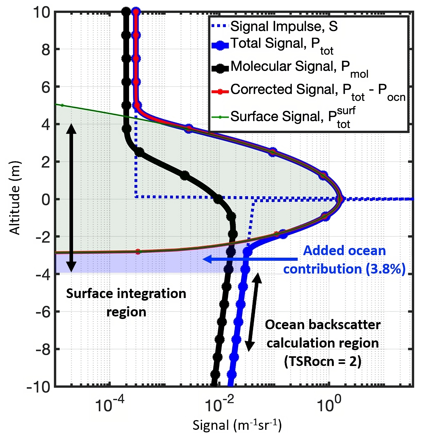
Figure 1Visualization of HSRL-2 measurement signals as described in Eqs. (5a), (5b), (6), (7a), and (7b). The dashed line denotes ideal total backscatter signal from the atmosphere, surface reflection, and the ocean subsurface. Blue and black lines denote measured signals from total and molecular scattering channels, respectively. Red and green lines show the ocean-corrected signal and the ocean surface backscatter, respectively. Dots indicate the altitudes of digitized samples. The sampling rate is 120 MHz, resulting in a vertical spacing of 1.25 m in the atmosphere and 0.94 m in the ocean.
It is seen from Fig. 1 and Eq. (7b) that the surface component of the measured signal Ptot is not localized to the surface but is instead spread above and below the surface via convolution with the system response function. The atmosphere and ocean components of Ptot are also impacted by the convolution, as is Pmol. Rearranging Eqs. (7a) and (7b) and integrating the total surface backscatter component over the full vertical extent of the system response function (i.e., to ±Δz), the surface response function can be eliminated in the representation of βsurf, as shown in Eq. (8).
Of course, the measurement that can be accessed is Ptot, not the surface component, . If Ptot were substituted for in Eq. (8), βsurf would be overestimated due to the contribution of ocean subsurface backscatter. The atmospheric contribution is negligible (i.e., < 0.05 %) and can be ignored. The magnitude of the contribution of the ocean subsurface scattering depends on the level of ocean particulate (hydrosol) as well as molecular seawater backscatter. The magnitude of this scattering relative to the surface backscatter can impact the retrieved surface wind speed accuracy. For example, at and assuming pure seawater (i.e., no hydrosols), the integrated total surface signal would be 5.7 % higher than the integrated surface backscatter. This results in a decrease of 0.75 m s−1 (−11 % error) in the estimated surface wind speed. At a 20 m s−1 surface wind speed, the error in the calculated surface wind speeds results in a decrease of 2.7 m s−1 (−14 % error). The ocean subsurface correction becomes less as the particulate scattering (or absorption) increases due to increased attenuation in the seawater and therefore contributes less over the integration window around the ocean surface. Therefore, the ocean subsurface contribution is higher for clear water compared to turbid water. For example, in the case illustrated in Fig. 1, the seawater particulate and molecular scattering are equal, resulting in a contribution of only 3.8 % to the integrated surface backscatter as compared to the case with no particulate scattering noted above (5.7 %). The atmospheric signal contribution is much less (∼ 100 times smaller) than the ocean subsurface signal, and therefore its contribution is considered negligible. Fortunately, the high vertical resolution of the HSRL-2 instrument enables the ocean subsurface contribution to be estimated. The separation of the molecular signal also enables estimation of the two-way transmittance, T2, and gain factor, Gmol, in Eq. (8).
For the HSRL-2 instrument, the two-way transmittance is determined directly from the measured molecular channel, Pmol. The two-way total (particulate and molecular attenuation) transmittance to the surface can be calculated as follows:
where F is the iodine vapor filter function (known from lab and in-flight calibration), is the molecular backscatter coefficient for the atmosphere (computed from pressure and temperature data from a reanalysis model), and is the range-scaled molecular channel signal near the ocean surface (where rns is the near-surface range). In practice, this is computed by averaging data from 60 to 180 m above the surface. This range is somewhat arbitrary but is chosen as a balance between ensuring that the signal does not include any of the surface reflectance and that the signal is low enough to capture most of the attenuation down to the surface. Substituting Eq. (9) into Eq. (8), one can solve for the surface backscatter,
To account for the ocean subsurface contributions to the measured signal, Eqs. (5a) and (5b) can be rearranged as
A benefit of the HSRL-2 retrieval algorithm is that one can use the molecular channel signal to determine the ocean signal near the surface (see Fig. 1). To determine the near-surface ocean signal, an estimate of the total ocean scattering ratio (TSR) is employed, which is the ratio of molecular plus hydrosol backscatter divided by molecular backscatter. An estimate of the near-surface TSR () is computed, using the quotient of the total and molecular channels () averaged over a small range of depths just below the depth at which the surface signal response goes to zero, as the following equation:
where Focn accounts for the spectral transmission of the molecular seawater backscatter through the iodine vapor filter and is determined via in-flight and laboratory calibrations. The ocean subsurface component of the total channel backscatter is estimated as the following equation:
Here the assumption is that the TSR is vertically constant near the surface over the 0.5 s (∼ 75 m horizontal resolution) integration of the lidar signals. Combining Eqs. (10), (11), and (13) and ignoring the atmospheric contribution to the total channel signal, one can compute the absolute surface backscatter using the two measured channels as
The use of the molecular channel in this way cancels out the absolute system gain constant (Gmol), provides an estimate of the two-way transmittance of the atmosphere, and enables subtraction of the ocean subsurface backscatter. It does not require precise knowledge of the system response function or any other assumptions. With Eq. (14), one can calculate the wave slope variance using Eq. (1) and then use Eqs. (2.1)–(2.3) to derive surface wind speeds.
In addition to the specular reflection from the surface, whitecaps or sea foam can increase the lidar backscatter signal. As noted in Josset et al. (2010b), the contribution of scattering by the whitecaps on the ocean surface has been treated as Lambertian scattering. There is a wavelength dependence of the scattering at longer wavelengths due to water absorption, based on measurements presented by Dierssen (2019) covering wavelengths from 0.4 to 2.5 µm. Measurements presented here are at 532 nm, a region of the visible spectrum where scattering from foam is relatively constant with wavelength. The contribution of whitecaps is typically modeled with a constant average reflectance and an effective-area-weighted fraction that varies with surface wind speed (Whitlock et al., 1982; Koepke, 1984; Gordon and Wang, 1994; Moore et al., 2000). Following Moore et al. (2000), we have estimated the average reflectance due to the whitecaps as a function of surface wind speed, and the difference becomes > 1 m s−1 for surface wind speeds > 15 m s−1 based on this relationship (Fig. 2). The main observation is that there are limited data (49 data points) above 13.3 m s−1 that can be compared to the dropsonde surface wind speeds to evaluate this relationship. Moreover, since the correction depends on surface wind speed, an iterative calculation is required to use this relationship, as the backscatter is dependent on wind speed.
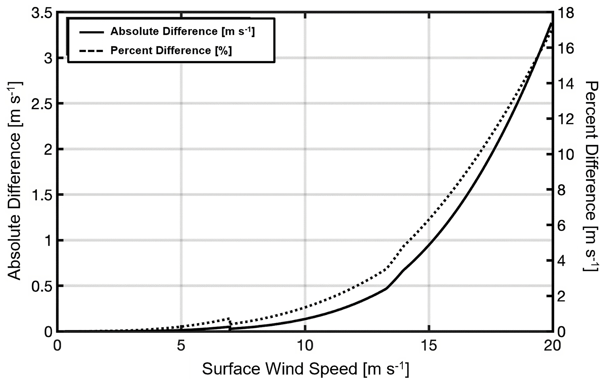
Figure 2Estimated absolute difference in calculated surface wind speed if reflectance from whitecaps is not included. The lidar surface backscatter is higher than the specular reflectance if whitecaps are present, which results in a lower estimated surface wind speed if not accounted for in the retrieval.
Alternatively, Hu et al. (2008) used a full month of CALIPSO-integrated surface depolarization ratio data (the ratio of the integrated cross-polarized channel to the integrated co-polarized channel across the surface) and applied an empirical correction to the reflectance that was determined using AMSR-E data as the ground-truth data set to increase the correlation of the data sets. The correlation was based on much more data than the ACTIVATE matchups between HSRL-2 and dropsondes, limiting the utility of a similar analysis with the HSRL-2. In addition, there are significant differences in the configurations of CALIPSO and HSRL-2 that limit implementation of the same empirical relationship. First, the CALIPSO integrated surface depolarization includes the subsurface contributions due to its 30 m vertical resolution, whereas the HSRL-2 surface depolarization is integrated over only a few meters, as shown in Fig. 1. Second, the CALIPSO data are based on global data, which are dominated by oligotrophic (clear) waters, whereas a significant fraction of the HSRL-2–dropsonde comparisons is from eutrophic and mesotrophic waters near the coast and along the shelf. Third, there is a significant difference in footprint size between HSRL-2 and CALIPSO (8 m versus 90 m), with the HSRL-2 instantaneous footprint area being greater than 2 orders of magnitude smaller and, considering the HSRL-2 along-track averaging (100 laser shots) compared to the CALIPSO single-shot data, greater than 1 order of magnitude smaller in terms of the area over which surface depolarization is integrated.
2.5 Collocation and statistical procedures
Since surface wind speeds are the focus of this study, first the dropsonde wind speed data points closest to 10 m (altitude of 11.56 ± 3.19 m for the 577 points) above sea level are recorded for each launch (multiple launches per flight) to allow meaningful comparison with the HSRL-2 surface wind speeds. Since one data point was taken per dropsonde for each flight, there are 160 recorded dropsonde measurements for 2020, 245 measurements for 2021, and 335 measurements for 2022. Then, the HSRL-2 surface wind speed retrieval closest in space and time to the corresponding dropsonde measurement is recorded. Collocation between the HSRL-2 and the dropsondes is constrained to below 30 km horizontally and to below 15 min temporally to remove outliers, while trying to maximize the number of data points to be used in the study. Further constraining these distance and time conditions would eliminate more data points with negligible improvement to the statistics, as shown by Figs. S1 and S2 in the Supplement. Due to missing data in the HSRL-2 data set and the removal of outliers based on collocation constraints, 577 data points are available for comparison between the dropsondes and the HSRL-2 (Fig. 3).
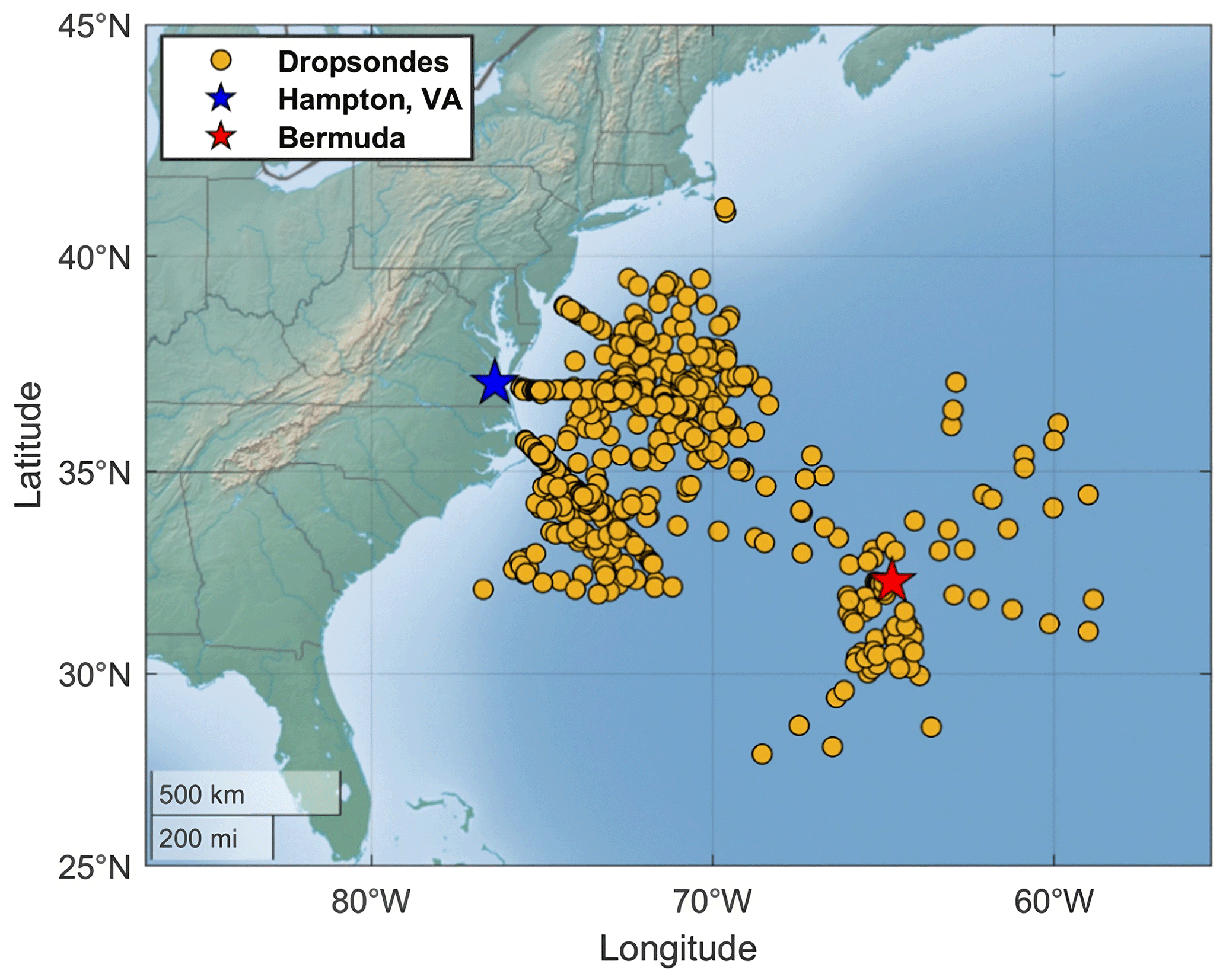
Figure 3Map of 577 ACTIVATE dropsondes launched from the King Air between 2020 and 2022, which are used to evaluate the HSRL-2 surface wind speed retrievals introduced in this study.
After the surface wind speed data are prepared using the procedure above, scatterplots, the correlation coefficient (r), linear regression, and ordinary least-squares bisector regression (OLS-bisector) are used to visually demonstrate how well HSRL-2 surface wind speed data match dropsonde data and to show any potential variability in the data. Since the OLS-bisector technique is less common than linear regression, a brief explanation of their differences is provided. In a linear regression, X is treated as the independent variable, while Y is treated as the dependent variable. In other words, one observes how Y varies with changes to fixed X values. An OLS-bisector is known as an error-in-variable regression technique, where X and Y are both dependent variables and thus both subject to error. An OLS-bisector regresses Y on X (standard OLS) and then regresses X on Y (inverse OLS), then bisects the angle of these two regression lines (Ricker, 1973). Although other error-in-variable techniques exist (e.g., Deming regression and orthogonal distance regression), the OLS-bisector technique was chosen because it calculates the error present in both data sets using the bisector rather than assuming an error a priori like the examples mentioned (Wu and Yu, 2018). After performing these regressions, histograms of surface wind speed deltas, which are defined as HSRL-2 surface wind speed minus dropsonde surface wind speed, are created to show the distribution and spread of the data more easily. The mean and standard deviation (SD) of the surface wind speed deltas are computed and then used to define the mean error (mean ± SD). This metric is used to evaluate how accurately the HSRL-2 retrieves surface wind speeds.
3.1 Case studies
Before delving into the HSRL-2–dropsonde surface wind speed intercomparisons in full statistical detail, surface wind speed data from two ACTIVATE research flights are analyzed: research flight 29 on 28 August 2020 and research flight 14 on 1 March 2020. These flights are analyzed to demonstrate the ability of the HSRL-2 to (1) provide profiles that show the spatial variability in surface wind speed over time, which are beneficial to observe phenomena like sea surface temperature dynamics and cloud evolution, and (2) sample the surface in broken cloud scenes, showing that the retrievals are not limited to cloud- and aerosol-free conditions like in Hu et al. (2008).
3.1.1 Research flight 29 on 28 August 2020
Research flight 29 was a nearly cloud-free day where an above-average number of dropsondes were launched, and the ACTIVATE aircraft were coordinated with the CALIPSO satellite overpass. These conditions allow for the examination of how the high horizontal spatial resolution of the HSRL-2 (∼ 75 m along the track as mentioned in Sect. 2.4) influences its retrievals and how the data can be used to track sea surface temperature (SST) gradients common to the WNAO (Painemal et al., 2021), as seen in Fig. 4. Note that Fig. 4a uses SST data from the Modern-Era Retrospective Analysis for Research and Applications, Version 2 (MERRA-2; Gelaro et al., 2017) to contextualize the SST gradients present in the WNAO, but no comparisons with MERRA-2 surface wind speed data are performed in this study.
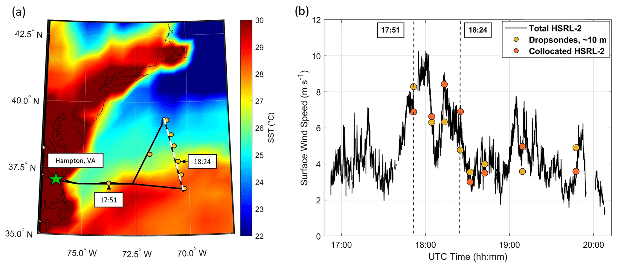
Figure 4(a) Flight map of the King Air (black line) and dropsondes (dark yellow circles) overlaid onto a map of MERRA-2 mean sea surface temperature (SST) data (GMAO, 2015) for research flight 29 on 28 August 2020. The dashed white line corresponds to the CALIPSO overpass coincident with the King Air flight path. Time stamps represent where the King Air crosses over sharp SST changes associated with the Gulf Stream. (b) Time series of surface wind speed data from HSRL-2 and dropsondes for the same flight, where the solid black line signifies total HSRL-2 surface wind speed data, and circles indicate collocated surface wind speed data points. Dashed black lines represent time stamps of interest as indicated in (a).
It is seen that changes in the HSRL-2 surface wind speeds (Fig. 4b) correspond to changes in SST (Fig. 4a), especially at 17:51 and 18:24 UTC (coordinated universal time; all instances of time in the text are in UTC). As the aircraft approaches and crosses the SST boundary at 17:51 (i.e., SST increasing), there is a corresponding increase in surface wind speeds. The reverse observation can be seen when the aircraft approaches and crosses the boundary at 18:24 (i.e., SST decreasing), where surface wind speeds noticeably decrease. Although further analysis is needed to rigorously examine the relationship between surface wind speed and SST, these observations show that the HSRL-2 has the high horizontal spatial resolution needed to probe the fine-scale variability in surface wind speeds and has the potential to improve atmospheric modeling of MABL processes. These profiles capture the spatial gradients in surface wind speeds that would otherwise not be available with the dropsondes alone, since these instruments can only take point measurements as they drop vertically to the surface and therefore cannot provide the horizontal spatial extent like the derived HSRL-2 surface wind speed product can.
3.1.2 Research flight 14 on 1 March 2020
Next, research flight 14 is shown in Fig. 5 to demonstrate the ability of the HSRL-2 to sample in broken cloud scenes. This flight, along with the associated morning flight on 1 March 2020, has been the subject of several studies owing to its coincidence with cold air outbreak conditions (see cloud streets in Fig. 5a) and a flight strategy that allowed for detailed characterization of the evolving aerosol–cloud system as a function of distance offshore (Seethala et al., 2021; Chen et al., 2022; Li et al., 2022; Tornow et al., 2022; Sorooshian et al., 2023). The morning flight focused on a location with very detailed characterization including stacked level flight legs (i.e., a “wall”), with the Falcon flying below, in, and above clouds and the King Air flying aloft to further characterize the same region. The afternoon flight consisted of both aircraft flying back to that same location, adjusting the sampling strategy to fly along the boundary layer wind direction in a quasi-Lagrangian fashion to keep studying the evolution of the air mass characterized in the morning. The afternoon flight is chosen because it shows the full range of cloud conditions from clear to completely overcast. Therefore, the HSRL-2 surface wind speed retrievals are able to be evaluated in this range of conditions.
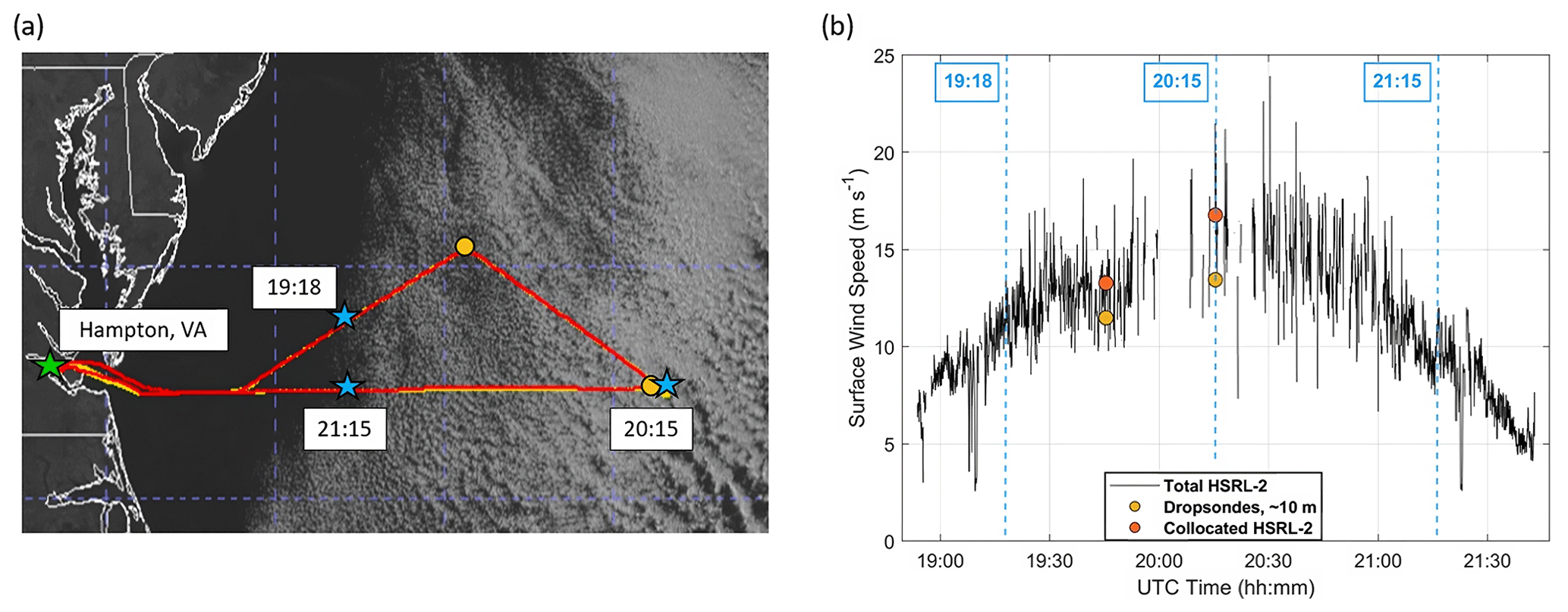
Figure 5(a) Flight map of the King Air (red line), Falcon (yellow line), and dropsondes (dark yellow circles) overlaid onto Geostationary Operational Environmental Satellite (GOES-16) cloud imagery for research flight 14 on 1 March 2020. Blue stars represent time stamps where the King Air crosses over from cloud-free to cloudy areas. (b) Time series of surface wind speed data from HSRL-2 and dropsondes for the same flight, where lines signify total HSRL-2 surface wind speed data, and circles indicate collocated surface wind speed data points. Dashed blue lines represent time stamps of interest as indicated in panel (a).
As the aircraft approaches the cloud scene at 19:18, there is a noticeable and steady increase in HSRL-2 surface wind speeds. The reverse observation is seen at 21:15, where the HSRL-2 surface wind speeds start to decrease steadily. As highlighted in the 28 August 2020 case study, the high horizontal spatial resolution of the HSRL-2 retrievals enables these spatial gradients to be observed. Another important takeaway is that the HSRL-2 is still able to sample the surface in cloud scenes, as seen by the almost-complete surface wind speed profile in Fig. 5b. Although a gap in data occurs at 20:15, where cloud cover is most substantial, some retrievals are still present in that area. The reason is that the HSRL-2 can probe the surface through gaps between clouds, allowing the surface wind speed retrievals to take place. Although the HSRL-2 retrievals would be unavailable in overcast cloud scenes, the ability of the instrument to sample the surface in broken cloud fields and not just aerosol- and cloud-free scenes is a significant benefit of the lidar and the HSRL technique.
3.2 HSRL-2–dropsonde comparisons
Now, the collocated HSRL-2 retrievals and dropsonde measurements of surface wind speed are compared, and the results are shown in Fig. 6.
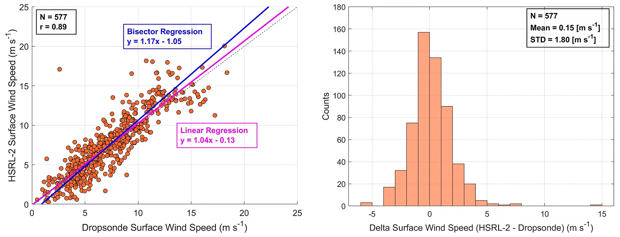
Figure 6Scatterplots with associated histograms for HSRL-2–dropsonde collocated surface wind speed data points using the ACTIVATE 2020–2022 data set. N represents the number of data points.
The comparison yields correlation coefficients of 0.89, slopes of 1.04 and 1.17, and y intercepts of −0.13 and −1.05 m s−1 for linear and bisector regressions, respectively. Note that the correlation coefficients are the same for the linear and bisector regressions throughout this analysis, so they are listed as one value throughout Sect. 3.2. Using the mean and SD values in the same figure, the mean error or accuracy of the HSRL-2 surface wind speed retrievals is 0.15 ± 1.80 m s−1. These results show that on average, the HSRL-2 slightly overestimates surface wind speeds and that the estimation can be off by about 2 m s−1 in either direction.
Now that the HSRL-2 retrievals have been broadly evaluated, Fig. 7 shows how their accuracy varies per 1 m s−1 interval in surface wind speed. This plot also provides the opportunity to compare the Hu et al. (2008) model with the models proposed by Cox and Munk (1954) and Wu (1990) to see if some of the error in the HSRL-2 retrievals can be attributed to model characteristics.
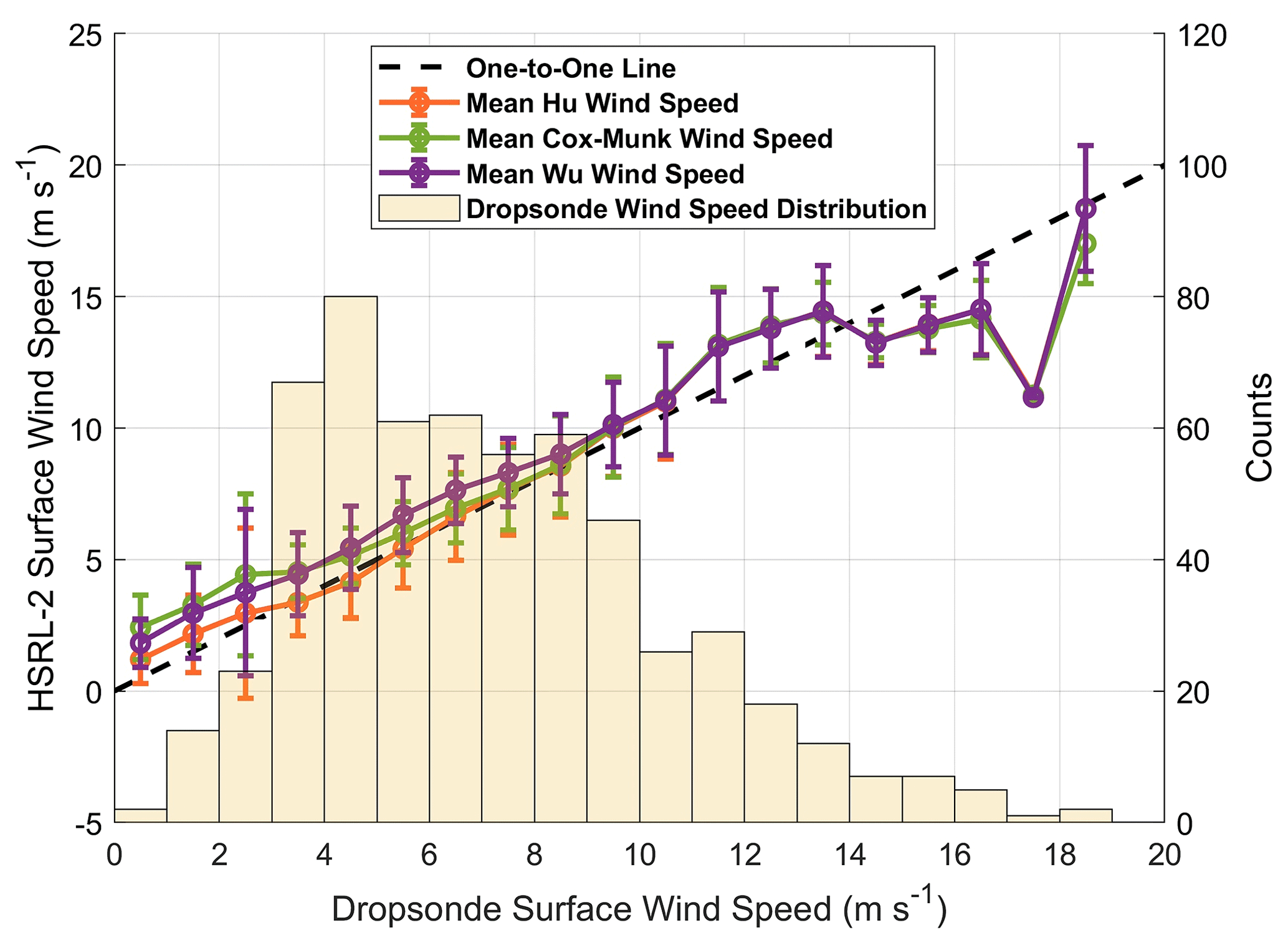
Figure 7HSRL-2 surface wind speed using the Hu, Cox–Munk, and Wu models versus mean dropsonde surface wind speed calculated per 1 m s−1 bin. A histogram of dropsonde surface wind speeds is also included to show their distribution.
It is seen that the mean Cox–Munk and Wu surface wind speed values are higher than the mean Hu values from 0 to 7 m s−1, showing that the Cox–Munk and Wu relationships overestimate dropsonde surface wind speeds more than the Hu relationship does. The variability (i.e., SD) around the mean per bin is similar between the three models, which is 1.59 m s−1 for Hu, 1.43 m s−1 for Cox–Munk, and 1.55 m s−1 for Wu, on average. Although similar, the SD of the Hu surface wind speeds found here is ∼ 0.4 m s−1 lower than the one found in Fig. 6. This could be attributed to an SD not being able to be calculated for the 17 to 18 m s−1 bin since it only contained one point.
Although it is apparent that the Cox–Munk and Wu retrievals overestimate dropsonde observations for surface wind speeds below 7 m s−1, it is still unclear which of the models performs better overall. Therefore, the y axis from Fig. 7 is converted to wave slope space, and the result of this modification is shown in Fig. 8. HSRL-2 wave slope is used because it directly reports the original measurements of surface reflectance rather than the estimated values of surface wind speed. Using the original data ensures that uncertainty is coming from the actual HSRL-2–dropsonde comparisons rather than from potential errors in the conversion from wave slope to surface wind speed.
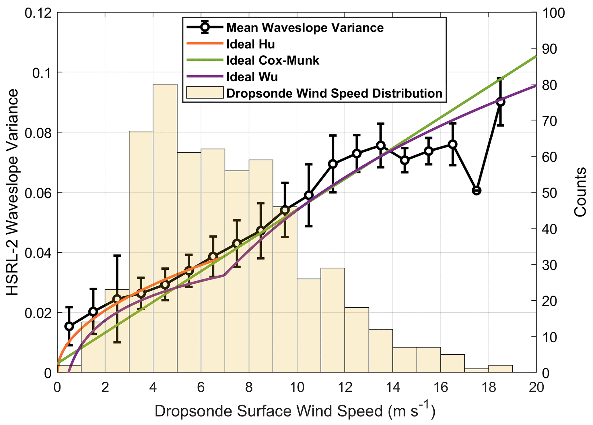
Figure 8HSRL-2 wave slope variance versus mean dropsonde surface wind speed calculated per 1 m s−1 bin. Ideal Hu, Cox–Munk, and Wu distributions are included to show how well observed dropsonde data match each parameterization. A histogram of dropsonde surface wind speeds is also included to show their distribution.
From Fig. 8, it is more easily seen how the dropsonde surface wind speed distribution compares with the Hu, Cox–Munk, and Wu parameterizations. Dropsonde surface wind speeds match the Hu and Cox–Munk parameterizations quite closely but not the Wu parameterization between 7 and 13.3 m s−1, although some divergence is seen above ∼ 10.5 m s−1. However, a critical observation that is more apparent in Fig. 8 than in Fig. 7 is how the dropsonde data most resemble the Hu distribution for surface wind speeds below 7 m s−1. This improvement is substantial, especially since most of the surface wind speeds in ACTIVATE fall into this category. Surface wind speeds above 13.3 m s−1 substantially diverge from all models, especially speeds above 16 m s−1. As mentioned previously, there are few surface wind speed observations in this category, so more measurements are necessary to make meaningful comparisons between the two data sets. Overall, Figs. 7 and 8 demonstrate the benefits of using the Hu parameterization in this study and why surface wind speeds above 13.3 m s−1 are not the main focus of the comparisons in this section. Further analysis is warranted to rigorously compare the performance of various surface reflectance models and potentially apply corrections (i.e., whitecap correction for surface wind speeds above 13.3 m s−1), but the aim of this paper is to evaluate the LARC HSRL-2 surface wind speed retrieval algorithm using the available ground-truth dropsonde measurements.
Now that the Hu relationship has been deemed the more effective model through the preliminary analysis shown in Figs. 7 and 8, a more rigorous statistical analysis is performed for surface wind speeds (1) below 7 m s−1 and (2) between 7 and 13.3 m s−1 to assess the overall accuracy of the HSRL-2 retrievals in these categories (Fig. 9).
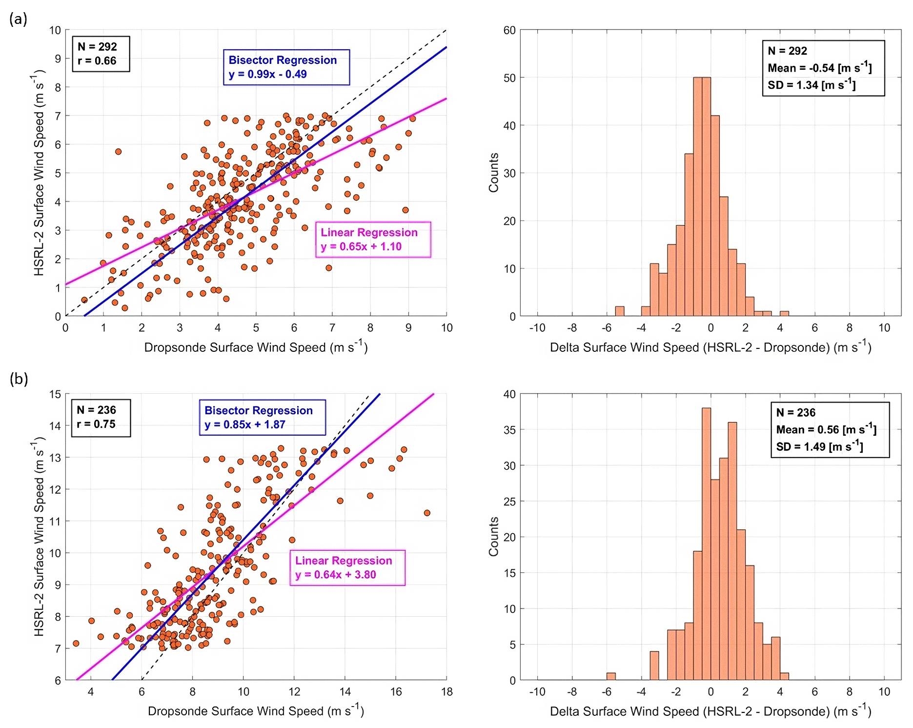
Figure 9Scatterplots with associated histograms for HSRL-2–dropsonde collocated surface wind speed data points for (a) surface wind speeds < 7 m s−1 and (b) surface wind speeds between 7 and 13.3 m s−1. Note that the x- and y-axis ranges vary to better showcase results in individual panels. N represents the number of data points.
Intercomparisons for surface wind speeds below 7 m s−1 (Fig. 9a) show correlation coefficients of 0.66, slopes of 0.65 and 0.99, and y intercepts of 1.10 and −0.49 m s−1 for linear and bisector regressions, respectively. The accuracy of the HSRL-2 retrievals is calculated to be −0.54 ± 1.34 m s−1, showing that the HSRL-2 on average underestimates surface wind speeds, and this estimation could vary by ± 1.34 m s−1. For surface wind speeds between 7 and 13.3 m s−1 (Fig. 9b), correlation coefficients of 0.75, slopes of 0.64 and 0.85, and y intercepts of 3.80 and 1.87 m s−1 are reported for linear and bisector regressions, respectively. The mean error of 0.56 ± 1.49 m s−1 shows that the HSRL-2 overpredicts surface wind speeds by about ∼ 0.5 m s−1 on average, with a variability of ± ∼ 1.5 m s−1. Therefore, the means from both categories average out to ∼ 0 m s−1 since they are approximately the same but in opposite directions. Separating the data into these categories highlights an important result that could not be seen in the cumulative data (Fig. 6): one can expect bias of up to ∼ 0.5 m s−1 in either direction and error of up to ∼ 1.5 m s−1 on average for most HSRL-2 surface wind speed retrievals in ACTIVATE.
The data are then divided into winter and summer deployments (dates provided in Sect. 2.1), as shown in Fig. 10, to assess the HSRL-2 retrieval accuracy in different seasons.
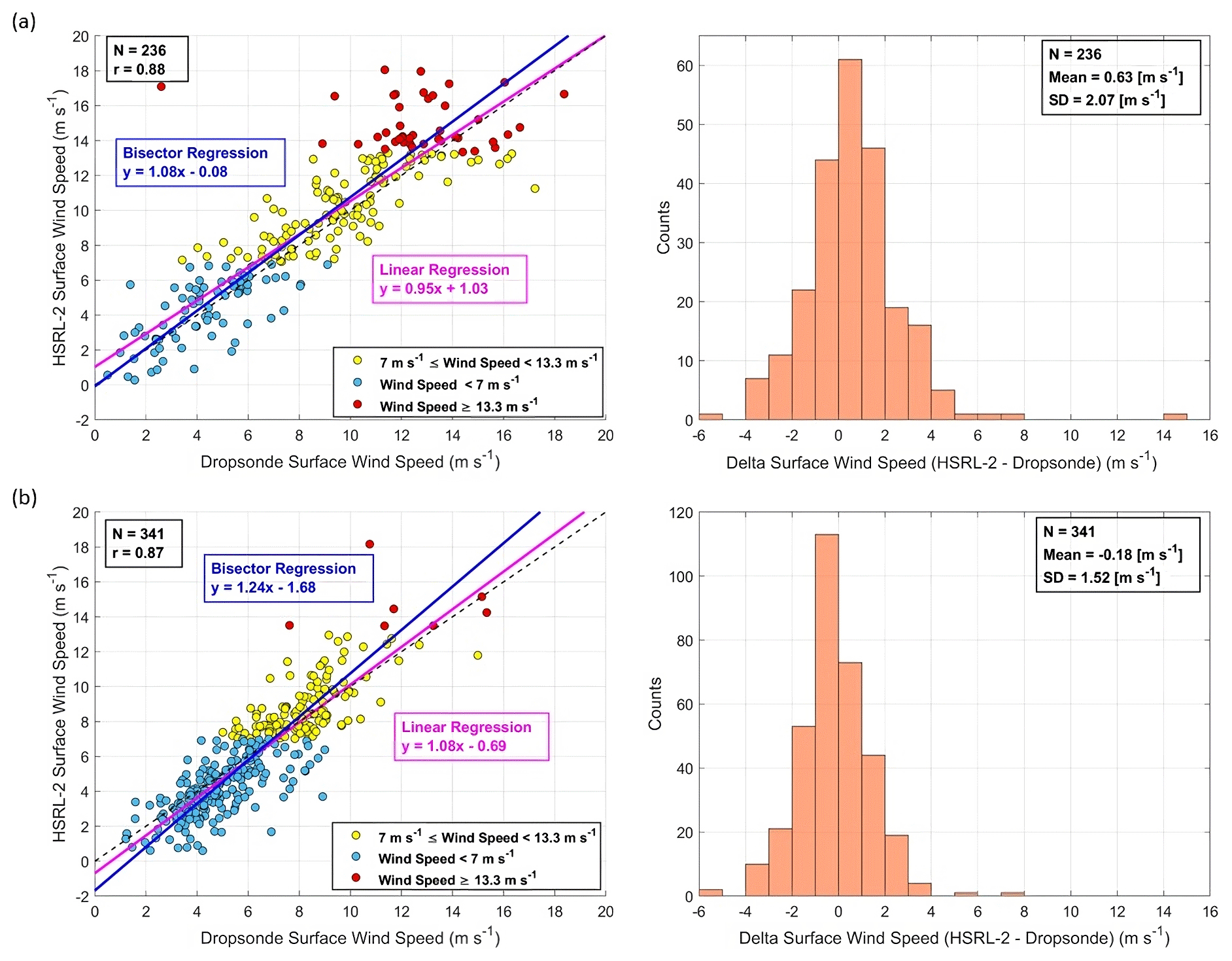
Figure 10Scatterplots with associated histograms for HSRL-2–dropsonde collocated surface wind speed data points for (a) winter and (b) summer deployments. Data are highlighted based on surface wind speed categories: , wind speed < 7 m s−1, and wind speed ≥ 13.3 m s−1. N represents the number of data points.
As seen in Fig. 10a, the winter surface wind speed intercomparisons show correlation coefficients of 0.88, slopes of 0.95 and 1.08, and y intercepts of 1.03 and −0.08 m s−1 for linear and bisector regressions, respectively. The summer surface wind speed intercomparisons (Fig. 10b) have correlations of 0.87, slopes of 1.08 and 1.24, and y intercepts of −0.69 and −1.68 m s−1. Finally, the mean errors for winter and summer, respectively, are reported as 0.63 ± 2.07 and −0.18 ± 1.52 m s−1. It is seen that the error in the HSRL-2 estimations of surface wind speeds is larger for winter than for summer, most likely due to the higher fraction of surface wind speeds above 13.3 m s−1 and lower fraction below 7 m s−1 in the winter. This observation makes sense because of the increased presence of clouds, precipitation, and whitecaps for the higher surface wind speeds observed in the winter. These observations show that HSRL-2 retrievals of surface wind speed are more accurate in the summer versus the winter. However, the HSRL-2 can still make numerous accurate retrievals, as shown by Fig. 10 and the 1 March 2020 research flight discussions. Caution must still be exercised when using data from days featuring turbulent meteorological conditions that could induce whitecaps and/or substantial cloud cover that could limit the HSRL-2 or that prevent the HSRL-2 from sampling the surface.
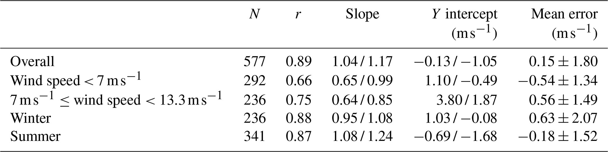
Statistics evaluating the HSRL-2 surface wind speed retrievals (Figs. 6, 9, and 10) are summarized in Table 1 for convenience.
Table 1Summary of all HSRL-2–dropsonde surface wind speed comparison statistics shown in Figs. 6, 9, and 10. The two values for slope and y intercept refer to those for the linear and bisector regressions, in that order. R values are the same for both linear and bisector regressions, so they are listed as one value.
This study introduces a new 10 m surface wind speed product from the NASA Langley Research Center (LARC) nadir-viewing High-Spectral-Resolution Lidar – Generation 2 (HSRL-2) instrument and demonstrates its use and accuracy. The HSRL-2 retrievals are evaluated using NCAR AVAPS dropsonde surface wind speed data collected during the NASA ACTIVATE field campaign. ACTIVATE featured the joint deployment of the HSRL-2 and AVAPS dropsondes during six deployments from 2020 to 2022, enabling the accuracy of the HSRL-2 surface wind speed retrievals to be assessed using coincident dropsonde measurements. Comparisons of HSRL-2 and dropsonde surface wind speeds show correlations of 0.89, slopes of 1.04 and 1.17, and y intercepts of −0.13 and −1.05 m s−1 for linear and bisector regressions, respectively. The accuracy of the HSRL-2 retrievals, as denoted by mean error, is calculated to be 0.15 ± 1.80 m s−1. It is also observed that the dropsonde surface wind speed measurements more closely match the Hu et al. (2008) wind speed–wave slope variance model than with the Cox and Munk (1954) and Wu (1990) models for surface wind speeds below 7 m s−1, which is an important finding because most ACTIVATE surface wind speeds fall into this category. After this overview of model performance, the HSRL-2 retrievals for surface wind speeds separated into the below 7 m s−1 and between 7 and 13.3 m s−1 categories are then evaluated in more detail. For surface wind speeds below 7 m s−1, correlations of 0.66, slopes of 0.65 and 0.99, and y intercepts of 1.10 and −0.49 m s−1 are found, and the accuracy of the retrievals is found to be −0.54 ± 1.34 m s−1. Surface wind speeds between 7 and 13.3 m s−1 show correlations of 0.75, slopes of 0.64 and 0.85, and y intercepts of 3.80 and 1.87 m s−1, and the retrieval accuracy is shown to be 0.56 ± 1.49 m s−1. Statistics are not reported for surface wind speeds above 13.3 m s−1 because there are too few points in this category to make meaningful comparisons. These results showcase an important observation not seen in the cumulative results, which is that the HSRL-2 estimates surface wind speeds with a bias of ± ∼ 0.5 m s−1 and an error of ± ∼ 1.5 m s−1. Lastly, the data are divided into winter and summer deployments (the dates denoted in Sect. 2.1) to assess how the HSRL-2 performs between seasons. The winter surface wind speed data comparisons show correlations of 0.88, slopes of 0.95 and 1.08, and y intercepts of 1.03 and −0.08 m s−1, and the summer data show correlations of 0.87, slopes of 1.08 and 1.24, and y intercepts of −0.69 and −1.68 m s−1 (linear and bisector regressions, respectively). The accuracy of the lidar retrievals is reported as 0.63 ± 2.07 and −0.18 ± 1.52 m s−1 for winter and summer, respectively. These findings show that HSRL-2 retrievals are more accurate in the summer than in the winter but still provide substantial (N= 236) and accurate surface wind speed data in winter as well.
This retrieval method offers a new path forward in airborne fieldwork for the acquisition of surface wind speed data at a high spatial (∼ 75 m along track) and time (0.5 s) resolution, as demonstrated by two case study flights (research flight 29 on 28 August 2020 and research flight 14 on 1 March 2020). The high horizontal spatial resolution of the HSRL-2 allows it to probe the fine-scale variability in surface wind speeds over time. As a result, the instrument provides near-continuous profiles of surface wind speeds over time that correspond to MABL phenomena such as SST dynamics and cloud evolution. Another important conclusion about the HSRL-2 surface retrievals is that the instrument can detect the surface in broken cloud scenes and is not limited to aerosol-free conditions like in Hu et al. (2008). Overall, having such data can benefit model assimilation efforts and consequently several scientific applications related to air–sea interactions, such as estimating heat fluxes, gas exchange, sea salt emissions and aerosol transport, and cloud life cycle.
Forthcoming work will continue assessments of surface wind speed measurements during ACTIVATE by comparing dropsonde data to in situ measurements taken by the Turbulent Air Motion Measurement System (TAMMS) on board the Falcon aircraft at its various altitude flight legs (between 120 m and 5 km; Thornhill et al., 2003). Additional work is also warranted to assess the surface wind speed retrievals performed by the other ACTIVATE remote sensor, the Research Scanning Polarimeter (RSP), to fully demonstrate the remote sensing capabilities of ACTIVATE.
ACTIVATE airborne data are available through https://doi.org/10.5067/SUBORBITAL/ACTIVATE/DATA001 (NASA Langley Research Center, 2020). MERRA-2 mean sea surface temperature data are taken from the 2 d 1 h Time-Averaged Single-Level Assimilation Surface Flux Diagnostics V5.12.4 (M2T1NXFLX) product found at https://doi.org/10.5067/7MCPBJ41Y0K6 (GMAO, 2015). GOES-16 data are from https://doi.org/10.5067/ASDC/SUBORBITAL/ACTIVATE-Satellite_1 (NASA/LARC/SD/ASDC, 2023).
The supplement related to this article is available online at: https://doi.org/10.5194/amt-17-3515-2024-supplement.
SD performed all analyses with input from all co-authors. SD, JWH, RAF, CAH, JAR, and AS prepared the paper with all co-authors involved in review and editing. TJS, DBH, STS, and CER conducted flight scientist duties on the King Air and helped with preparation and deployment of dropsondes. JWH, RAF, MAF, CAH, BLC, DBH, STS, TJS, and EC were responsible for the HSRL-2 instrumentation, and KLT, CER, and HV were responsible for the NCAR AVAPS dropsonde instrumentation collection and for the subsequent archival of the surface wind speed data sets needed to conduct this analysis. JWH, JAR, YH, RAF, CAH, and BLC all contributed to the formulation of the HSRL-2 retrieval algorithm.
The contact author has declared that none of the authors has any competing interests.
Publisher's note: Copernicus Publications remains neutral with regard to jurisdictional claims made in the text, published maps, institutional affiliations, or any other geographical representation in this paper. While Copernicus Publications makes every effort to include appropriate place names, the final responsibility lies with the authors.
This work was funded by ACTIVATE, a NASA Earth Venture Suborbital-3 (EVS-3) investigation funded by the NASA Earth Science Division and managed through the Earth System Science Pathfinder Program Office. We thank the pilots and aircraft maintenance personnel from the NASA Langley Research Services Directorate for successfully conducting ACTIVATE flights. The MERRA-2 1 h Time-Averaged Single-Level Assimilation Surface Flux Diagnostics V5.12.4 (M2T1NXFLX) data used in this effort were acquired as part of the activities of the NASA Science Mission Directorate and are archived and distributed by the Goddard Earth Sciences (GES) Data and Information Services Center (DISC).
This research has been supported by the National Aeronautics and Space Administration, NASA Headquarters (grant no. 80NSSC19K0442).
This paper was edited by Ad Stoffelen and reviewed by Lev Labzovskii and one anonymous referee.
Aldhaif, A. M., Lopez, D. H., Dadashazar, H., and Sorooshian, A.: Sources, frequency, and chemical nature of dust events impacting the United States East Coast, Atmos. Environ., 231, 117456, https://doi.org/10.1016/j.atmosenv.2020.117456, 2020.
Bedka, K. M., Nehrir, A. R., Kavaya, M., Barton-Grimley, R., Beaubien, M., Carroll, B., Collins, J., Cooney, J., Emmitt, G. D., Greco, S., Kooi, S., Lee, T., Liu, Z., Rodier, S., and Skofronick-Jackson, G.: Airborne lidar observations of wind, water vapor, and aerosol profiles during the NASA Aeolus calibration and validation (Cal/Val) test flight campaign, Atmos. Meas. Tech., 14, 4305–4334, https://doi.org/10.5194/amt-14-4305-2021, 2021.
Bellouin, N., Quaas, J., Gryspeerdt, E., Kinne, S., Stier, P., Watson-Parris, D., Boucher, O., Carslaw, K. S., Christensen, M., Daniau, A.-L., Dufresne, J.-L., Feingold, G., Fiedler, S., Forster, P., Gettelman, A., Haywood, J. M., Lohmann, U., Malavelle, F., Mauritsen, T., McCoy, D. T., Myhre, G., Mülmenstädt, J., Neubauer, D., Possner, A., Rugenstein, M., Sato, Y., Schulz, M., Schwartz, S. E., Sourdeval, O., Storelvmo, T., Toll, V., Winker, D., and Stevens, B.: Bounding Global Aerosol Radiative Forcing of Climate Change, Rev. Geophys., 58, e2019RG000660, https://doi.org/10.1029/2019RG000660, 2020.
Brunke, M. A., Cutler, L., Urzua, R. D., Corral, A. F., Crosbie, E., Hair, J., Hostetler, C., Kirschler, S., Larson, V., Li, X.-Y., Ma, P.-L., Minke, A., Moore, R., Robinson, C. E., Scarino, A. J., Schlosser, J., Shook, M., Sorooshian, A., Lee Thornhill, K., Voigt, C., Wan, H., Wang, H., Winstead, E., Zeng, X., Zhang, S., and Ziemba, L. D.: Aircraft Observations of Turbulence in Cloudy and Cloud-Free Boundary Layers Over the Western North Atlantic Ocean From ACTIVATE and Implications for the Earth System Model Evaluation and Development, J. Geophys. Res.-Atmos., 127, e2022JD036480, https://doi.org/10.1029/2022JD036480, 2022.
Burton, S. P., Ferrare, R. A., Hostetler, C. A., Hair, J. W., Rogers, R. R., Obland, M. D., Butler, C. F., Cook, A. L., Harper, D. B., and Froyd, K. D.: Aerosol classification using airborne High Spectral Resolution Lidar measurements – methodology and examples, Atmos. Meas. Tech., 5, 73–98, https://doi.org/10.5194/amt-5-73-2012, 2012.
Burton, S. P., Hostetler, C. A., Cook, A. L., Hair, J. W., Seaman, S. T., Scola, S., Harper, D. B., Smith, J. A., Fenn, M. A., Ferrare, R. A., Saide, P. E., Chemyakin, E. V., and Müller, D.: Calibration of a high spectral resolution lidar using a Michelson interferometer, with data examples from ORACLES, Appl. Optics, 57, 6061–6075, https://doi.org/10.1364/AO.57.006061, 2018.
Carvalho, D.: An Assessment of NASA's GMAO MERRA-2 Reanalysis Surface Winds, J. Climate, 32, 8261–8281, https://doi.org/10.1175/JCLI-D-19-0199.1, 2019.
Chemyakin, E., Stamnes, S., Hair, J., Burton, S. P., Bell, A., Hostetler, C., Ferrare, R., Chowdhary, J., Moore, R., Ziemba, L., Crosbie, E., Robinson, C., Shook, M., Thornhill, L., Winstead, E., Hu, Y., van Diedenhoven, B., and Cairns, B.: Efficient single-scattering look-up table for lidar and polarimeter water cloud studies, Opt. Lett., 48, 13–16, https://doi.org/10.1364/OL.474282, 2023.
Chen, J., Wang, H., Li, X., Painemal, D., Sorooshian, A., Thornhill, K. L., Robinson, C., and Shingler, T.: Impact of Meteorological Factors on the Mesoscale Morphology of Cloud Streets during a Cold-Air Outbreak over the Western North Atlantic, J. Atmos. Sci., 79, 2863–2879, https://doi.org/10.1175/JAS-D-22-0034.1, 2022.
Christoudias, T., Pozzer, A., and Lelieveld, J.: Influence of the North Atlantic Oscillation on air pollution transport, Atmos. Chem. Phys., 12, 869–877, https://doi.org/10.5194/acp-12-869-2012, 2012.
Corral, A. F., Choi, Y., Crosbie, E., Dadashazar, H., DiGangi, J. P., Diskin, G. S., Fenn, M., Harper, D. B., Kirschler, S., Liu, H., Moore, R. H., Nowak, J. B., Scarino, A. J., Seaman, S., Shingler, T., Shook, M. A., Thornhill, K. L., Voigt, C., Zhang, B., Ziemba, L. D., and Sorooshian, A.: Cold Air Outbreaks Promote New Particle Formation Off the U. S. East Coast, Geophys. Res. Lett., 49, e2021GL096073, https://doi.org/10.1029/2021GL096073, 2022.
Cox, C. and Munk, W.: Measurement of the Roughness of the Sea Surface from Photographs of the Sun's Glitter, J. Opt. Soc. Am., 44, 838–850, https://doi.org/10.1364/JOSA.44.000838, 1954.
Creilson, J. K., Fishman, J., and Wozniak, A. E.: Intercontinental transport of tropospheric ozone: a study of its seasonal variability across the North Atlantic utilizing tropospheric ozone residuals and its relationship to the North Atlantic Oscillation, Atmos. Chem. Phys., 3, 2053–2066, https://doi.org/10.5194/acp-3-2053-2003, 2003.
Dadashazar, H., Painemal, D., Alipanah, M., Brunke, M., Chellappan, S., Corral, A. F., Crosbie, E., Kirschler, S., Liu, H., Moore, R. H., Robinson, C., Scarino, A. J., Shook, M., Sinclair, K., Thornhill, K. L., Voigt, C., Wang, H., Winstead, E., Zeng, X., Ziemba, L., Zuidema, P., and Sorooshian, A.: Cloud drop number concentrations over the western North Atlantic Ocean: seasonal cycle, aerosol interrelationships, and other influential factors, Atmos. Chem. Phys., 21, 10499–10526, https://doi.org/10.5194/acp-21-10499-2021, 2021.
Dierssen, H. M.: Hyperspectral Measurements, Parameterizations, and Atmospheric Correction of Whitecaps and Foam From Visible to Shortwave Infrared for Ocean Color Remote Sensing, Front. Earth Sci., 7, 14, https://doi.org/10.3389/feart.2019.00014, 2019.
Ferrare, R., Hair, J., Hostetler, C., Shingler, T., Burton, S. P., Fenn, M., Clayton, M., Scarino, A. J., Harper, D., Seaman, S., Cook, A., Crosbie, E., Winstead, E., Ziemba, L., Thornhill, L., Robinson, C., Moore, R., Vaughan, M., Sorooshian, A., Schlosser, J. S., Liu, H., Zhang, B., Diskin, G., DiGangi, J., Nowak, J., Choi, Y., Zuidema, P., and Chellappan, S.: Airborne HSRL-2 measurements of elevated aerosol depolarization associated with non-spherical sea salt, Frontiers in Remote Sensing, 4, 1143944, https://doi.org/10.3389/frsen.2023.1143944, 2023.
Gelaro, R., McCarty, W., Suárez, M. J., Todling, R., Molod, A., Takacs, L., Randles, C. A., Darmenov, A., Bosilovich, M. G., Reichle, R., Wargan, K., Coy, L., Cullather, R., Draper, C., Akella, S., Buchard, V., Conaty, A., da Silva, A. M., Gu, W., Kim, G.-K., Koster, R., Lucchesi, R., Merkova, D., Nielsen, J. E., Partyka, G., Pawson, S., Putman, W., Rienecker, M., Schubert, S. D., Sienkiewicz, M., and Zhao, B.: The Modern-Era Retrospective Analysis for Research and Applications, Version 2 (MERRA-2), J. Climate, 30, 5419–5454, https://doi.org/10.1175/JCLI-D-16-0758.1, 2017.
GMAO (Global Modeling and Assimilation Office): MERRA-2 tavg1_2d_flx_Nx: 2d,1-Hourly,Time-Averaged,Single-Level,Assimilation,Surface Flux Diagnostics V5.12.4, Goddard Earth Sciences Data and Information Services Center (GES DISC) [data set], Greenbelt, MD, USA, https://doi.org/10.5067/7MCPBJ41Y0K6, 2015.
Gordon, H. R. and Wang, M.: Influence of oceanic whitecaps on atmospheric correction of ocean-color sensors, Appl. Optics, 33, 7754–7763, https://doi.org/10.1364/AO.33.007754, 1994.
Hair, J. W., Hostetler, C. A., Cook, A. L., Harper, D. B., Ferrare, R. A., Mack, T. L., Welch, W., Izquierdo, L. R., and Hovis, F. E.: Airborne High Spectral Resolution Lidar for profiling aerosol optical properties, Appl. Optics, 47, 6734–6752, https://doi.org/10.1364/AO.47.006734, 2008.
Hu, Y., Stamnes, K., Vaughan, M., Pelon, J., Weimer, C., Wu, D., Cisewski, M., Sun, W., Yang, P., Lin, B., Omar, A., Flittner, D., Hostetler, C., Trepte, C., Winker, D., Gibson, G., and Santa-Maria, M.: Sea surface wind speed estimation from space-based lidar measurements, Atmos. Chem. Phys., 8, 3593–3601, https://doi.org/10.5194/acp-8-3593-2008, 2008.
Josset, D., Pelon, J., Protat, A., and Flamant, C.: New approach to determine aerosol optical depth from combined CALIPSO and CloudSat ocean surface echoes, Geophys. Res. Lett., 35, L10805, https://doi.org/10.1029/2008GL033442, 2008.
Josset, D., Pelon, J., and Hu, Y.: Multi-Instrument Calibration Method Based on a Multiwavelength Ocean Surface Model, IEEE Geosci. Remote S., 7, 195–199, https://doi.org/10.1109/LGRS.2009.2030906, 2010a.
Josset, D., Zhai, P.-W., Hu, Y., Pelon, J., and Lucker, P. L.: Lidar equation for ocean surface and subsurface, Opt. Express, 18, 20862–20875, https://doi.org/10.1364/OE.18.020862, 2010b.
Kiliyanpilakkil, V. P. and Meskhidze, N.: Deriving the effect of wind speed on clean marine aerosol optical properties using the A-Train satellites, Atmos. Chem. Phys., 11, 11401–11413, https://doi.org/10.5194/acp-11-11401-2011, 2011.
Kirschler, S., Voigt, C., Anderson, B., Campos Braga, R., Chen, G., Corral, A. F., Crosbie, E., Dadashazar, H., Ferrare, R. A., Hahn, V., Hendricks, J., Kaufmann, S., Moore, R., Pöhlker, M. L., Robinson, C., Scarino, A. J., Schollmayer, D., Shook, M. A., Thornhill, K. L., Winstead, E., Ziemba, L. D., and Sorooshian, A.: Seasonal updraft speeds change cloud droplet number concentrations in low-level clouds over the western North Atlantic, Atmos. Chem. Phys., 22, 8299–8319, https://doi.org/10.5194/acp-22-8299-2022, 2022.
Koepke, P.: Effective reflectance of oceanic whitecaps, Appl. Optics, 23, 1816–1824, https://doi.org/10.1364/AO.23.001816, 1984.
Labzovskii, L. D., van Zadelhoff, G. J., Tilstra, L. G., de Kloe, J., Donovan, D. P., and Stoffelen, A.: High sensitivity of Aeolus UV surface returns to surface reflectivity, Sci. Rep.-UK, 13, 17552, https://doi.org/10.1038/s41598-023-44525-5, 2023.
Lamb, P. J. and Peppler, R. A.: North Atlantic Oscillation: Concept and an Application, B. Am. Meteorol. Soc., 68, 1218–1225, https://doi.org/10.1175/1520-0477(1987)068<1218:NAOCAA>2.0.CO;2, 1987.
Li, Q., Jacob, D. J., Bey, I., Palmer, P. I., Duncan, B. N., Field, B. D., Martin, R. V., Fiore, A. M., Yantosca, R. M., Parrish, D. D., Simmonds, P. G., and Oltmans, S. J.: Transatlantic transport of pollution and its effects on surface ozone in Europe and North America, J. Geophys. Res.-Atmos., 107, ACH 4-1–ACH 4-21, https://doi.org/10.1029/2001JD001422, 2002.
Li, X.-Y., Wang, H., Chen, J., Endo, S., George, G., Cairns, B., Chellappan, S., Zeng, X., Kirschler, S., Voigt, C., Sorooshian, A., Crosbie, E., Chen, G., Ferrare, R. A., Gustafson, W. I., Hair, J. W., Kleb, M. M., Liu, H., Moore, R., Painemal, D., Robinson, C., Scarino, A. J., Shook, M., Shingler, T. J., Thornhill, K. L., Tornow, F., Xiao, H., Ziemba, L. D., and Zuidema, P.: Large-Eddy Simulations of Marine Boundary Layer Clouds Associated with Cold-Air Outbreaks during the ACTIVATE Campaign. Part I: Case Setup and Sensitivities to Large-Scale Forcings, J. Atmos. Sci., 79, 73–100, https://doi.org/10.1175/JAS-D-21-0123.1, 2022.
Li, Z., Lemmerz, C., Paffrath, U., Reitebuch, O., and Witschas, B.: Airborne Doppler Lidar Investigation of Sea Surface Reflectance at a 355 nm Ultraviolet Wavelength, J. Atmos. Ocean. Tech., 27, 693–704, https://doi.org/10.1175/2009JTECHA1302.1, 2010.
Mardi, A. H., Dadashazar, H., Painemal, D., Shingler, T., Seaman, S. T., Fenn, M. A., Hostetler, C. A., and Sorooshian, A.: Biomass Burning Over the United States East Coast and Western North Atlantic Ocean: Implications for Clouds and Air Quality, J. Geophys. Res.-Atmos., 126, e2021JD034916, https://doi.org/10.1029/2021JD034916, 2021.
Martin, C. and Suhr, I.: NCAR/EOL Atmospheric Sounding Processing ENvironment (ASPEN) software, Version 3.4.5, Earth Observing Laboratory [code], https://www.eol.ucar.edu/content/aspen (last access: 10 February 2024), 2021.
Moore, K. D., Voss, K. J., and Gordon, H. R.: Spectral reflectance of whitecaps: Their contribution to water-leaving radiance, J. Geophys. Res.-Oceans, 105, 6493–6499, https://doi.org/10.1029/1999JC900334, 2000.
Murphy, A. and Hu, Y.: Retrieving Aerosol Optical Depth and High Spatial Resolution Ocean Surface Wind Speed From CALIPSO: A Neural Network Approach, Frontiers in Remote Sensing, 1, 614029, https://doi.org/10.3389/frsen.2020.614029, 2021.
Nair, A. K. M. and Rajeev, K.: Multiyear CloudSat and CALIPSO Observations of the Dependence of Cloud Vertical Distribution on Sea Surface Temperature and Tropospheric Dynamics, J. Climate, 27, 672–683, https://doi.org/10.1175/JCLI-D-13-00062.1, 2014.
NASA Langley Research Center: Aerosol Cloud MeTeorology Interactions oVer the western ATlantic Experiment Data, Atmospheric Science Data Center (ASDC) [data set], Hampton, VA, USA, https://doi.org/10.5067/SUBORBITAL/ACTIVATE/DATA001, 2020.
NASA/LARC/SD/ASDC: ACTIVATE GOES-16 Supplementary Data Products, NASA Langley Atmospheric Science Data Center DAAC [data set], https://doi.org/10.5067/ASDC/SUBORBITAL/ACTIVATE-Satellite_1, 2023.
Neukermans, G., Harmel, T., Galí, M., Rudorff, N., Chowdhary, J., Dubovik, O., Hostetler, C., Hu, Y., Jamet, C., Knobelspiesse, K., Lehahn, Y., Litvinov, P., Sayer, A. M., Ward, B., Boss, E., Koren, I., and Miller, L. A.: Harnessing remote sensing to address critical science questions on ocean-atmosphere interactions, Elementa: Science of the Anthropocene, 6, 1–46, https://doi.org/10.1525/elementa.331, 2018.
Painemal, D., Corral, A. F., Sorooshian, A., Brunke, M. A., Chellappan, S., Afzali Gorooh, V., Ham, S.-H., O'Neill, L., Smith Jr., W. L., Tselioudis, G., Wang, H., Zeng, X., and Zuidema, P.: An Overview of Atmospheric Features Over the Western North Atlantic Ocean and North American East Coast–Part 2: Circulation, Boundary Layer, and Clouds, J. Geophys. Res.-Atmos., 126, e2020JD033423, https://doi.org/10.1029/2020JD033423, 2021.
Painemal, D., Chellappan, S., Smith Jr., W. L., Spangenberg, D., Park, J. M., Ackerman, A., Chen, J., Crosbie, E., Ferrare, R., Hair, J., Kirschler, S., Li, X.-Y., McComiskey, A., Moore, R. H., Sanchez, K., Sorooshian, A., Tornow, F., Voigt, C., Wang, H., Winstead, E., Zeng, X., Ziemba, L., and Zuidema, P.: Wintertime Synoptic Patterns of Midlatitude Boundary Layer Clouds Over the Western North Atlantic: Climatology and Insights From In Situ ACTIVATE Observations, J. Geophys. Res.-Atmos., 128, e2022JD037725, https://doi.org/10.1029/2022JD037725, 2023.
Paiva, V., Kampel, M., and Camayo, R.: Comparison of Multiple Surface Ocean Wind Products with Buoy Data over Blue Amazon (Brazilian Continental Margin), Adv. Meteorol., 2021, 6680626, https://doi.org/10.1155/2021/6680626, 2021.
Ricker, W. E.: Linear Regressions in Fishery Research, J. Fish. Res. Board Can., 30, 409–434, https://doi.org/10.1139/f73-072, 1973.
Scarino, A. J., Obland, M. D., Fast, J. D., Burton, S. P., Ferrare, R. A., Hostetler, C. A., Berg, L. K., Lefer, B., Haman, C., Hair, J. W., Rogers, R. R., Butler, C., Cook, A. L., and Harper, D. B.: Comparison of mixed layer heights from airborne high spectral resolution lidar, ground-based measurements, and the WRF-Chem model during CalNex and CARES, Atmos. Chem. Phys., 14, 5547–5560, https://doi.org/10.5194/acp-14-5547-2014, 2014.
Schlosser, J. S., Stamnes, S., Burton, S. P., Cairns, B., Crosbie, E., Van Diedenhoven, B., Diskin, G., Dmitrovic, S., Ferrare, R., Hair, J. W., Hostetler, C. A., Hu, Y., Liu, X., Moore, R. H., Shingler, T., Shook, M. A., Thornhill, K. L., Winstead, E., Ziemba, L., and Sorooshian, A.: Polarimeter + Lidar–Derived Aerosol Particle Number Concentration, Frontiers in Remote Sensing, 3, 885332, https://doi.org/10.3389/frsen.2022.885332, 2022.
Schulien, J. A., Behrenfeld, M. J., Hair, J. W., Hostetler, C. A., and Twardowski, M. S.: Vertically- resolved phytoplankton carbon and net primary production from a high spectral resolution lidar, Opt. Express, 25, 13577–13587, https://doi.org/10.1364/OE.25.013577, 2017.
Seethala, C., Zuidema, P., Edson, J., Brunke, M., Chen, G., Li, X.-Y., Painemal, D., Robinson, C., Shingler, T., Shook, M., Sorooshian, A., Thornhill, L., Tornow, F., Wang, H., Zeng, X., and Ziemba, L.: On Assessing ERA5 and MERRA2 Representations of Cold-Air Outbreaks Across the Gulf Stream, Geophys. Res. Lett., 48, e2021GL094364, https://doi.org/10.1029/2021GL094364, 2021.
Sorooshian, A., Anderson, B., Bauer, S. E., Braun, R. A., Cairns, B., Crosbie, E., Dadashazar, H., Diskin, G., Ferrare, R., Flagan, R. C., Hair, J., Hostetler, C., Jonsson, H. H., Kleb, M. M., Liu, H., MacDonald, A. B., McComiskey, A., Moore, R., Painemal, D., Russell, L. M., Seinfeld, J. H., Shook, M., Smith, W. L., Thornhill, K., Tselioudis, G., Wang, H., Zeng, X., Zhang, B., Ziemba, L., and Zuidema, P.: Aerosol–Cloud–Meteorology Interaction Airborne Field Investigations: Using Lessons Learned from the U. S. West Coast in the Design of ACTIVATE off the U. S. East Coast, B. Am. Meteorol. Soc., 100, 1511–1528, https://doi.org/10.1175/BAMS-D-18-0100.1, 2019.
Sorooshian, A., Corral, A. F., Braun, R. A., Cairns, B., Crosbie, E., Ferrare, R., Hair, J., Kleb, M. M., Hossein Mardi, A., Maring, H., McComiskey, A., Moore, R., Painemal, D., Scarino, A. J., Schlosser, J., Shingler, T., Shook, M., Wang, H., Zeng, X., Ziemba, L., and Zuidema, P.: Atmospheric Research Over the Western North Atlantic Ocean Region and North American East Coast: A Review of Past Work and Challenges Ahead, J. Geophys. Res.-Atmos., 125, e2019JD031626, https://doi.org/10.1029/2019JD031626, 2020.
Sorooshian, A., Alexandrov, M. D., Bell, A. D., Bennett, R., Betito, G., Burton, S. P., Buzanowicz, M. E., Cairns, B., Chemyakin, E. V., Chen, G., Choi, Y., Collister, B. L., Cook, A. L., Corral, A. F., Crosbie, E. C., van Diedenhoven, B., DiGangi, J. P., Diskin, G. S., Dmitrovic, S., Edwards, E.-L., Fenn, M. A., Ferrare, R. A., van Gilst, D., Hair, J. W., Harper, D. B., Hilario, M. R. A., Hostetler, C. A., Jester, N., Jones, M., Kirschler, S., Kleb, M. M., Kusterer, J. M., Leavor, S., Lee, J. W., Liu, H., McCauley, K., Moore, R. H., Nied, J., Notari, A., Nowak, J. B., Painemal, D., Phillips, K. E., Robinson, C. E., Scarino, A. J., Schlosser, J. S., Seaman, S. T., Seethala, C., Shingler, T. J., Shook, M. A., Sinclair, K. A., Smith Jr., W. L., Spangenberg, D. A., Stamnes, S. A., Thornhill, K. L., Voigt, C., Vömel, H., Wasilewski, A. P., Wang, H., Winstead, E. L., Zeider, K., Zeng, X., Zhang, B., Ziemba, L. D., and Zuidema, P.: Spatially coordinated airborne data and complementary products for aerosol, gas, cloud, and meteorological studies: the NASA ACTIVATE dataset, Earth Syst. Sci. Data, 15, 3419–3472, https://doi.org/10.5194/essd-15-3419-2023, 2023.
Sun, K., Dai, G., Wu, S., Reitebuch, O., Baars, H., Liu, J., and Zhang, S.: Effect of wind speed on marine aerosol optical properties over remote oceans with use of spaceborne lidar observations, Atmos. Chem. Phys., 24, 4389–4409, https://doi.org/10.5194/acp-24-4389-2024, 2024.
Thornhill, K. L., Anderson, B. E., Barrick, J. D. W., Bagwell, D. R., Friesen, R., and Lenschow, D. H.: Air motion intercomparison flights during Transport and Chemical Evolution in the Pacific (TRACE-P)/ACE-ASIA, J. Geophys. Res.-Atmos., 108, 9001, https://doi.org/10.1029/2002JD003108, 2003.
Tornow, F., Ackerman, A. S., Fridlind, A. M., Cairns, B., Crosbie, E. C., Kirschler, S., Moore, R. H., Painemal, D., Robinson, C. E., Seethala, C., Shook, M. A., Voigt, C., Winstead, E. L., Ziemba, L. D., Zuidema, P., and Sorooshian, A.: Dilution of Boundary Layer Cloud Condensation Nucleus Concentrations by Free Tropospheric Entrainment During Marine Cold Air Outbreaks, Geophys. Res. Lett., 49, e2022GL098444, https://doi.org/10.1029/2022GL098444, 2022.
van Diedenhoven, B., Hasekamp, O. P., Cairns, B., Schuster, G. L., Stamnes, S., Shook, M., and Ziemba, L.: Remote sensing of aerosol water fraction, dry size distribution and soluble fraction using multi-angle, multi-spectral polarimetry, Atmos. Meas. Tech., 15, 7411–7434, https://doi.org/10.5194/amt-15-7411-2022, 2022.
Venkata, S. L. and Reagan, J. A.: Aerosol Retrievals from CALIPSO Lidar Ocean Surface Returns, Remote Sens.-Basel, 8, 1006, https://doi.org/10.3390/rs8121006, 2016.
Vömel, H. and Dunion, J.: Chapter 10 – Aircraft dropsonde campaigns, in: Field Measurements for Passive Environmental Remote Sensing, edited by: Nalli, N. R., Elsevier, 185–194, https://doi.org/10.1016/B978-0-12-823953-7.00021-6, 2023.
Vömel, H., Goodstein, M., Tudor, L., Witte, J., Fuchs-Stone, Ž., Sentić, S., Raymond, D., Martinez-Claros, J., Juračić, A., Maithel, V., and Whitaker, J. W.: High-resolution in situ observations of atmospheric thermodynamics using dropsondes during the Organization of Tropical East Pacific Convection (OTREC) field campaign, Earth Syst. Sci. Data, 13, 1107–1117, https://doi.org/10.5194/essd-13-1107-2021, 2021.
Whitlock, C. H., Bartlett, D. S., and Gurganus, E. A.: Sea foam reflectance and influence on optimum wavelength for remote sensing of ocean aerosols, Geophys. Res. Lett., 9, 719–722, 1982.
Wu, C. and Yu, J. Z.: Evaluation of linear regression techniques for atmospheric applications: the importance of appropriate weighting, Atmos. Meas. Tech., 11, 1233–1250, https://doi.org/10.5194/amt-11-1233-2018, 2018.
Wu, J.: Mean square slopes of the wind-disturbed water surface, their magnitude, directionality, and composition, Radio Sci., 25, 37–48, https://doi.org/10.1029/RS025i001p00037, 1990.