the Creative Commons Attribution 4.0 License.
the Creative Commons Attribution 4.0 License.
 | 13 Jun 2024
Estimating the refractivity bias of FORMOSAT-7/COSMIC-2 Global Navigation Satellite System (GNSS) radio occultation in the deep troposphere
Gia Huan Pham
Shu-Chih Yang
Chih-Chien Chang
Shu-Ya Chen
Cheng Yung Huang
FORMOSAT-7/COSMIC-2 radio occultation (RO) measurements show promise for observing the deep troposphere and for providing critical information on the Earth's planetary boundary layer (PBL). However, refractivity retrieved in the low troposphere can have severe biases under certain thermodynamic conditions. This research examines the characteristics of the deep tropospheric biases and presents methods for estimating the region-dependent refractivity bias using statistical regression models. The results show that the biases have characteristics that vary over land and oceans. With substantial correlation between local spectral width (LSW) and bias, the LSW-based bias estimation model can explain the general pattern of the refractivity bias but with deficiencies in measuring the bias in the ducting regions and in certain areas over land. The estimation model involving the relationship with temperature and specific humidity (TQ) can capture the large biases associated with ducting. Finally, a minimum variance estimation that combines the LSW and TQ provides the most accurate estimation of the refractivity bias.
- Article
(18086 KB) - Full-text XML
- BibTeX
- EndNote


Global Navigation Satellite System (GNSS) radio occultation (RO) observations have become a critical data source in atmospheric applications, particularly numerical weather prediction (NWP; e.g., Healy, 2008; Rennie, 2010; Cucurull et al., 2007, 2017; Lien et al., 2021). Low-Earth-orbiting (LEO) satellites receive radio signals from GNSS transmitters, which bend due to atmospheric density changes. Information on the bending angle can be obtained with the GNSS RO technique, and then the atmospheric refractivity is further derived using Abel inversion. Since the RO technique measures the signal phase delay, it is not affected by clouds or rainfall. The RO profile is an all-weather observation with a high vertical resolution.
The RO observations, bending angle, and refractivity measure vertical gradients in atmospheric density, a function of temperature, moisture, and pressure (Kuo et al., 2004). RO observations provide information on temperature (stratosphere and upper troposphere) and moisture (lower troposphere) with low noise and low systematic errors (biases), which make them useful in atmospheric research (Eyre, 2008). Several GNSS RO missions, e.g., the FORMOSAT-3/Constellation Observing System for Meteorology, Ionosphere, and Climate (FS3/C), FORMOSAT-7/COSMIC-2 (FS7/C2), Meteorological Operational satellite (MetOp), Gravity Recovery And Climate Experiment (GRACE), Satellite de Aplicaciones Cientifico-C (SAC-C), X-band TerraSAR satellite (TerraSAR-X), and Korea Multi-Purpose Satellite-5 (KOMPSAT-5) have provided much RO data for NWP. Many studies have illustrated the positive impact of assimilating RO observations, such as the operational forecast systems at the European Centre for Medium-Range Weather Forecasts (ECMWF; Healy, 2014), the NCEP/Environmental Modeling Center (EMC; Cucurull et al., 2007), and the Taiwan Central Weather Administration (CWA; Lien et al., 2021). Moreover, studies have been initiated recently to investigate the potential of assimilating the large volume of commercial RO data from Spire, and the benefits can be identified in weather forecasting (Bowler, 2020a). In addition to improving global NWP, studies have also confirmed that assimilating RO observations improves severe weather prediction, particularly for tropical cyclones and heavy rainfall (e.g., Chen et al., 2020; 2021a, b, 2022; Chang and Yang, 2022; Yang et al., 2014).
As the successor to FS3/C, the FS7/C2 mission was launched in 2019 with support from the Taiwan National Space Agency (TASA) and the United States National Oceanic and Atmospheric Administration (NOAA) and National Science Foundation. The number of profiles obtained by FS7/C2 is approximately 3 times greater than that of FS3/C since FS7/C2 has dense coverage over the tropics and subtropics (Chen et al., 2021c). Compared with FS3/C, FS7/C2 has a higher signal-to-noise ratio (SNR), wider bandwidth, and a better open-loop (OL) tracking model. These advantages enable the retrieval of more data from RO signals penetrating the moist troposphere and give the ability to detect the planetary boundary layer (PBL) and super-refraction (SR) over the top of the PBL (Schreiner et al., 2020; Sokolovskiy et al., 2024). Chen et al. (2021c) showed that the data availability of the FS7/C2 RO profiles under 1 km is 5 times greater than that of the FS3/C profiles over a 6-month range. Anthes et al. (2022) noted that the penetration rate of RO profiles is high even under extremely moist conditions and near tropical cyclones. The ability to penetrate deep into the atmosphere makes RO measurements ideal for studying the PBL. The PBL is directly influenced by any exchange of energy, momentum, and mass between the Earth's surface and the atmosphere, and thus its characteristics are crucial for weather and climate variabilities.
However, the use of GNSS RO in the lower atmosphere still produces errors when radio rays pass through areas with strong vertical or horizontal refractivity gradients. It is known that negative biases in refractivity exist in the lower troposphere, especially in the tropics (Rocken et al., 1997). The implementation of open-loop tracking (Sokolovskiy, 2001) and the use of the holographic retrieval method largely reduce the negative refractivity bias (REFB) in lower troposphere in earlier generation RO missions. “Radioholographic” methods such as the canonical transform (CT) method (Gorbunov, 2002), Full Spectrum Inversion (FSI) (Jensen et al., 2003) and phase matching (PM) (Jensen et al., 2004) largely solve the multipath issue resulting from the “strong” refractivity gradient. Still, negative REFB can arise in the deep troposphere from multiple causes, as summarized by Feng et al. (2020) and Wang et al. (2020). A common cause (but not the only one) of negative biases in the lower troposphere is ducting (Sokolovskiy, 2003; Ao et al., 2003; Xie et al., 2010). When the vertical gradient of refractivity exceeds a critical value of −157 N units per km (Lopez, 2009), ducting occurs and rays are trapped inside the ducting layer. In the presence of ducting, the singularity problem in the Abel transforms leads to a non-unique inversion problem. Thus, the Abel inversion results in a negative bias refractivity below the ducting layers (Sokolovskiy, 2003). Feng et al. (2020) reported that climatological locations agree well with the areas of high ducting frequency, mainly over the subtropical eastern oceans. Furthermore, non-ducting-related biases exist in the RO data. Error associated with low SNR in the complex, moist lower troposphere may cause negative biases in bending angles and refractivity. Another potential source is that the propagation of radio waves in a medium with random refractivity irregularities can also cause biases (Gorbunov et al., 2015). In regard to the assimilation of RO data, quality control (QC) is applied to reject the RO data if the observation or the corresponding background is suspected to be affected by super-refraction. The rejection rate is high below 2 km due to the negative bias, which could also discard valuable information for data assimilation. To increase the value of RO data in the lower atmosphere, this study aims to examine the characteristics of the REFBs with the FS7/C2 RO data in more detail and proposes methodologies to estimate them.
Previous research has demonstrated that the negative REFB in the atmospheric boundary layer ABL can be recognized and estimated using canonical transform approximations (Sokolovskiy, 2003) and can be reconstructed in the presence of ducting conditions (Xie et al., 2006). Based on Xie et al. (2006), Wang et al. (2017) developed an optimal estimation of negative bias using precipitable water (PW) observations from Advanced Microwave Scanning Radiometer from the EOS (AMSR-E) data. Wang et al. (2020) further proposed a bias estimation algorithm by generating a candidate set of modeled ducting profiles. The one with the vertical gradient of the reflected bending angle closest to the observed profile is taken as the bias-corrected profile. However, there are some limitations to these methods, such that they only correct for ducting-related bias, and the grazing signal of the bending measurement is needed. For the RO observation error, the local spectral width (LSW), which measures the uncertainty in the RO bending angle, has been used to indicate the quality of the individual RO profiles. The LSW represents the errors caused by the nonspherical symmetry of refractivity in the moist troposphere (Gorbunov et al., 2006; Sokolovskiy et al., 2010). The use of RO observations in data assimilation is improved by considering the LSW parameter in the QC procedure (Liu et al., 2018) or in dynamic estimation of RO error in the lower troposphere (Zhang et al. 2023). Liu et al. (2018) showed that both uncertainties and biases were related to LSW. Sjoberg et al. (2023) recently showed a strong statistical correlation between lower-tropospheric uncertainties and LSW. They mentioned that they found a correlation between biases and LSW as well but did not provide details. Furthermore, Bowler (2020b) proposed estimating RO errors with information on mean temperatures below 20 km. These results suggest that variations in LSW, temperature, and humidity are related to the bias. Thus, we developed statistical models that adaptively consider the biases associated within each RO profile using LSW, temperature, and water vapor.
We first investigate the characteristics of the FS7/C2 RO REFB and establish regression-based bias estimation algorithms. Two types of algorithms are examined. One is based on the physical LSW parameter, and the other is related to thermodynamic variables (temperature and water vapor). By comparing the results of the estimated bias, we can identify how they link to the characteristics of each participating variable. Finally, a bias correction method for the RO profile in the lower troposphere is proposed by combining the two bias estimation algorithms. We expect that this new algorithm can be used for different aspects, such as improving the products of temperature and moisture profiles retrieved from the refractivity in the moist lower troposphere (Chen et al., 2020), defining the PBL height (Xie, 2014), and estimating precipitable water vapor (Lien et al., 2024). Furthermore, for the data assimilation (DA) systems that assimilate the RO refractivity, it is expected that the RO data in the deep troposphere can be better exploited using the bias estimation as a QC flag or by assimilating the calibrated refractivity profiles.
The remaining portions of this paper are organized as follows. Section 2 provides the data information and methods for estimating the REFB. Section 3 discusses the general characteristics of bias and its sensitivities with respect to different variables and land/sea conditions. Section 4 presents the results of bias estimation algorithms. Finally, the summary and conclusion are provided in Sect. 5.
2.1 GNSS RO FS7/C2 and ECMWF data
This study uses the FS7/C2 RO atmospheric profiles (atmPrf) and wet products (wetPf2) processed by the Taiwan Data Processing Center (TDPC). The study period is from 1 December 2019 to 29 February 2020, before the FS7/C2 data were assimilated into the ECMWF analysis. All RO profiles are distributed between 45° N and 45° S due to the low inclination orbits of the FS7/C2 satellites. A total of 244 853 profiles with the flag of “good data” are selected during the periods, and only data below the height of 25 km are used to focus on the bias characteristics in the troposphere. The data quality of the FS7/C2 constellation is improved compared to FS3/COSMIC (FS3/C) due to the use of the advanced RO receiver and post-processing with open-loop tracking. Most of the profiles show a deeper penetration with depths below 1 km, and the penetration rate is 40 % higher than that of FS3/C (Chen et al., 2021c). Figure 1 shows the number of profiles that penetrate below 1.5 km above mean sea level (a.m.s.l.) during the selected periods. The FS7/C2 data are mostly in tropical areas and have more profiles penetrating below 1.5 km over oceans than over land.
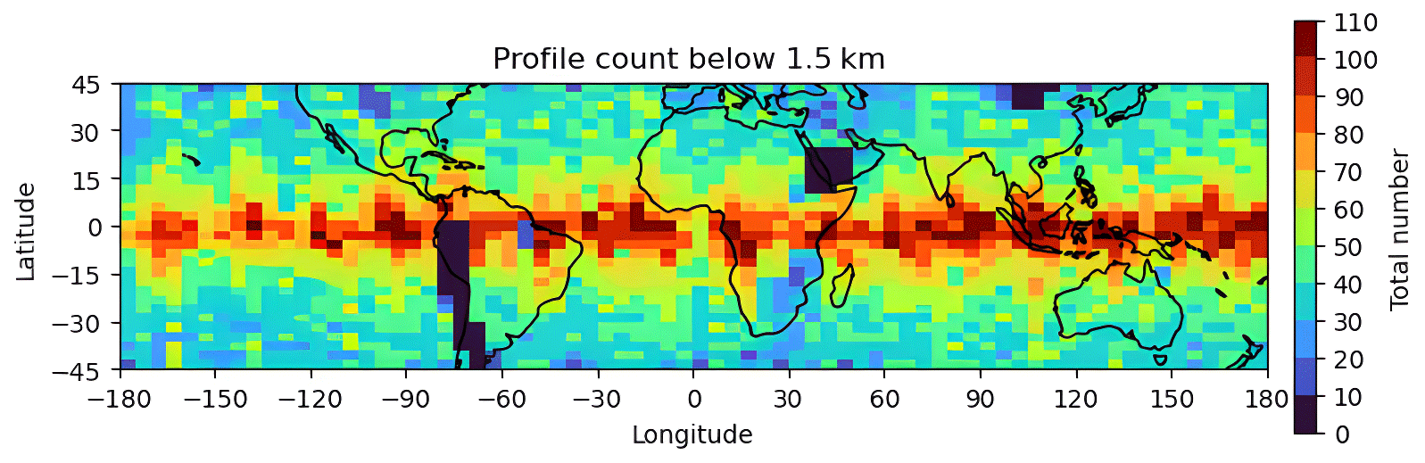
Figure 1Number of FS7/C2 RO profiles below 1.5 km in height during the study period (unit: number of profiles).
The ECMWF atmospheric reanalysis (ERA5, https://www.ecmwf.int/en/forecasts/access-forecasts/access-archive-datasets, last access: 10 March 2022) is used as the reference RO profile. The hourly ERA5 reanalysis in the study period has a horizontal resolution of 0.25° × 0.25° with 37 pressure levels ranging from 1000 to 1 hPa. Variable geopotential, temperature, and specific humidity are selected. Since the time of the RO data is precise in minutes, we rounded the time of the RO profiles to the nearest hour. The ERA5 profiles are derived by interpolating the reanalysis horizontally and vertically to the location and vertical levels of the RO atmPrf. The RO REFB is defined as the difference between the FS7/C2 and the ERA5 RO reference at each level. This assumes that the ERA5 refractivities are close to the truth. These biases are referred to as the real biases in this paper. Nevertheless, it is possible that ERA5 may carry its own biases, which will not be discussed in this study.
To construct the statistical models, the predictors are LSW, temperature (T), and specific humidity (Q). The LSW, available in the atmPrf data, is calculated from the width of the spectrum during the RO processing (Liu et al., 2018). T and Q, available in the wetPf2 data, are computed from a one-dimensional variational (1D-Var) retrieval algorithm using the ECMWF 12 h forecast as a prior factor (Wee et al., 2022).
2.2 Statistical models for bias estimation
Two polynomial regression models are developed to estimate the REFB using predictors associated with different attributions of the observational error in GNSS RO data. The first model uses LSW/2 as the predictor, and the other uses temperature (T) and specific humidity (Q) as the predictors. Liu et al. (2018) used a linear function of LSW/2 to illustrate the FS3/C dynamic error variance in the bending angle and refractivity, and the scaling factor for LSW approximates the root mean square of random error in the bending angle (Liu et al. (2018) assuming a Gaussian spectrum (Sirmans and Bumgarner, 1975). Following Liu et al. (2018), we use the variable LSW/2 and modify this relationship to a polynomial regression. The other bias estimation model is established using the thermodynamic variables to emphasize the impact of the thermodynamic structure on REFB in the deep troposphere. The two polynomial regression models are referred to as the LSW and TQ estimators, respectively. The LSW represents the RO inversion uncertainty, and T and Q represent the impact of the thermodynamic structure on REFB within the ABL. Each of these variables is expected to partly explain the characteristics of the bias.
In each estimator, the order of the polynomial is optimized using the R-squared and mean squared error metrics to assess the goodness-of-fit performance. The polynomial regression is performed with the training data, which is 80 % of the total data, and the rest (20 %) of the data are used for evaluating the regression performance. To derive a robust regression model, independent regression fitting is repeated five times by replacing the training (testing) data with different 80 % (20 %) subsets of the data so that the testing data from the five experiments eventually cover the whole data set. The regression model with the best-fitting performance for both training data and testing data is chosen as the optimal one. Given that our goal is to construct regional-dependent estimators to consider the spatial variation in the REFB, we group the RO refractivity profiles from 45° N to 45° S into 5° longitude × 3° latitude boxes (Fig. 1), and the regression-based REFB estimators are built into each box. In total, there are 72 × 30 boxes. The boxes are defined by considering that the number of available RO profiles below 1.5 km should be at least 10 profiles in each box to conduct the regression training and testing. With the 3 months of data used in our study, choosing testing data lower than 20 % of the total data results in a very coarse resolution of the boxes. On the other hand, choosing any number larger than 20 % would sacrifice the amount of data that can train a reliable regression model. We note that all profile data below 1.5 km are used first (80 % for training and 20 % for testing) to determine the order of the LSW-based regression model and the optimal combination of the multivariable (T and Q) regression model.
For the LSW estimator, a second-order polynomial is chosen based on the R-squared metric. Afterwards, a second-order polynomial regression is constructed for an individual box. Equation (1) shows the formula of the LSW estimator in the ith box,
where ui, the predictand, is the REFB; xi is the LSW/2; and are the regression coefficients. Although the biases related to the signal tracking or multipath are much reduced after the implementation of open-loop tracking and the radio-holographic retrieval method, we expect that LSW can partially capture the biases inherited from the bending angle.
A similar procedure is applied to derive a multivariable polynomial regression model, with T and Q obtained from the 1D-Var analysis of the RO wet products (Wee et al., 2022) as the predictors. For consistency, the real REFB originally defined with the atmPrf will be interpolated to the same levels of the wetPf2. No REFB, T or Q are collected if the wetPf2 profiles terminate above 1.5 km a.m.s.l. Before fitting, T and Q are standardized as
where χ represents a normalized quantity ranging between 0 and 1, and xi is the original value of Q or T in the ith box. Given two variables, there are different combinations of order and interaction terms (the multivariable polynomial function has the form of , where m and l are the order of variables y and z, respectively, and bm,l is the regression coefficient). For this application, the mean squared error (MSE) is used to determine the optimal fitting formula given that R-squared is comparable when higher order terms are included. The optimal multivariable polynomial regression model has the form
where ui is REFB, yi is the normalized Q, zi is the normalized T, and are the regression coefficients. Considering the quadratic term of moisture is essential. The R-squared (MSE) value increases (decreases) from 0.535 (37.044) with the yi and yizi terms to 0.732 (26.610) with the term.
We further apply the minimum variance estimation (MVE; Clarizia et al., 2014) to combine the results from the LSW and TQ estimators. This approach has the advantage of having a smaller root mean square error (RMSE) than either the LSW estimation or the TQ estimation. The MVE is built to linearly combine the estimations so that the new estimation has the minimum error variance
where u is the vector of the individual estimated refractivity bias and m is the vector of the combination coefficients. One of the advantages of this combination is that m is derived considering the error covariance matrix of individual bias estimators.
where 1 is a vector with all elements equal to one, K is the dimension of m (K=2 in our application), C−1 is the inverse of the covariance matrix between the individual estimation errors, and are the elements of C−1.
The element of the error covariance matrix C is expressed as , where ui and uj are the ith and jth bias estimations, respectively, and ut is the real bias.
3.1 General characteristics of REFB
Figure 2a shows the profile of the averaged REFB and its standard deviation from 0 to 25 km. RO data have significant biases in comparison to the ERA5 reference, especially in the low troposphere. The bias is evident below 5 km and is largest at the surface with an amplitude of approximately −11 N units. Given the large variations in moisture and temperature in the low troposphere, the standard deviation below 2 km increases as the height decreases. Notably, although the total number of profiles quickly decreases below 5 km (Fig. 2b), there remain enough data for near-surface statistical evaluation, with about a 40 % penetration rate at 0.5 km in reference to the total number of profiles at 10 km (Fig. 2c). The mean LSW (red line in Fig. 2a) also increases sharply as the height decreases, with two peaks (at the surface and near 2 km).
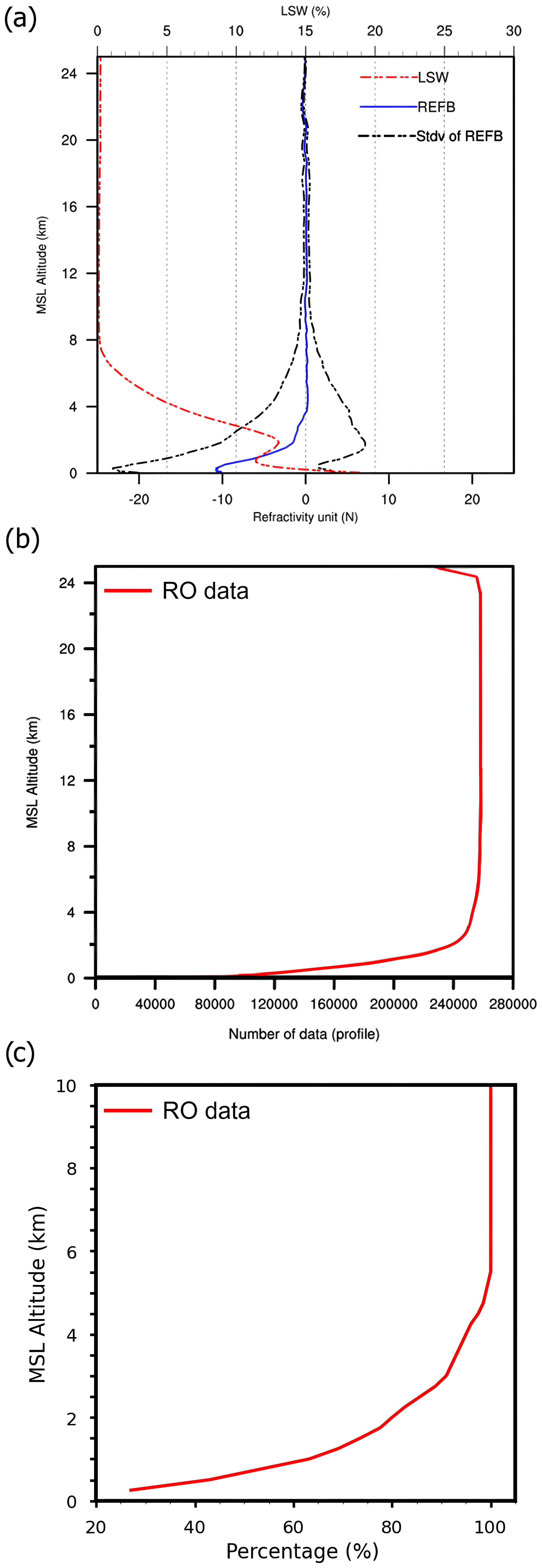
Figure 2 (a) Mean and standard deviation of REFB and mean LSW as a function of height. (b) The amount of available RO data and (c) the percentage of profiles as a function of height in reference to the total number at 10 km. The RO data are from 1 December 2019 to 29 February 2020.
Figure 3a shows the latitudinal cross-section of the REFB. The largest values of REFB are below 5 km in the subtropics and tropics and slightly shifted to the Southern Hemisphere due to the austral summer. The opposite pattern, which has a high bias shifted to the Northern Hemisphere, is also seen in the data from June to August 2020 (not shown). This result indicates the general dependence of the distribution of REFB on the seasonal temperature and water vapor structure. Similar to the REFB pattern, large LSW occurs mainly in the tropics, tilting toward the Southern Hemisphere with the maximum near the surface (Fig. 3b). This finding illustrates that LSW variation can be related to the REFB to some extent. Moreover, other high LSW values are located a few kilometers above the surface of the Southern Hemisphere. The increased LSW above 2 km could be caused by common inversion layers in the troposphere above oceans (Sokolovskiy et al., 2014). Another effect that could be considered is the influence of convective clouds just above moist oceans (Yang et al., 2016). The large LSW near the surface in Fig. 3b reflects the ability of FS7/C2 to penetrate deep into the moist troposphere of the tropics. However, this surface maximum was not seen in the study of Zhang et al. (2023) using FS3/C data in August 2008.
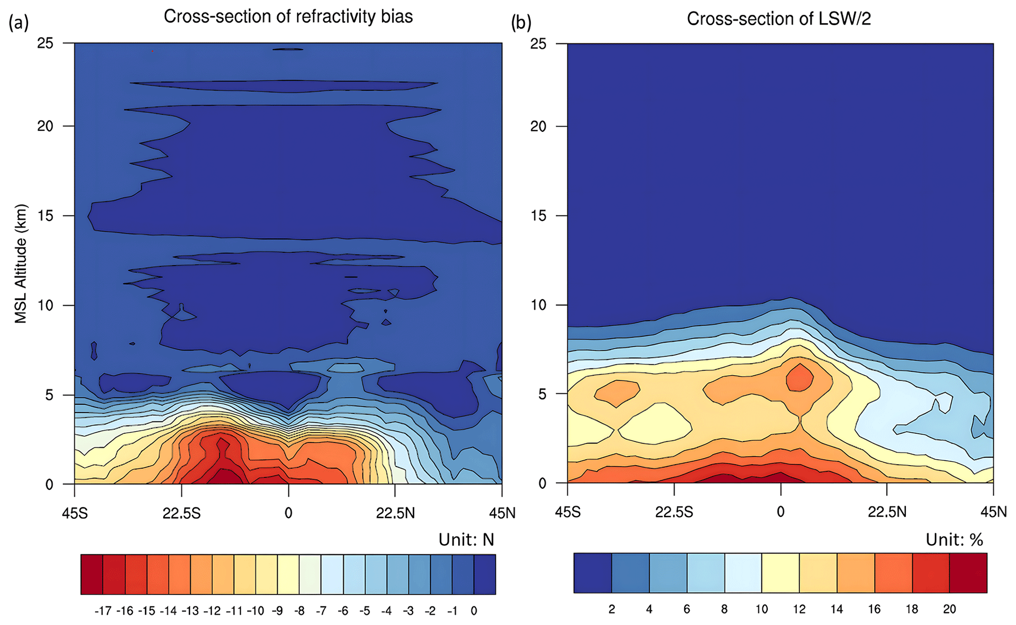
Figure 3The cross-sections of (a) zonal mean REFB and (b) mean LSW/2 from 1 December 2019 to 29 February 2020.
3.2 Dependence on geography and thermodynamic conditions
We further examine the dependence of the REFB on land and oceanic thermodynamic conditions. Figure 4 compares REFB between land and ocean, together with its standard deviation (SD) and LSW. Both REFB and LSW below 4 km are somewhat larger over oceans, and the REFB extends to higher altitudes (Fig. 4c vs. Fig. 4d) with a greater vertical gradient of REFB below 2 km. The magnitudes of mean REFB and SD above 2 km are comparable over land and ocean. The shape of the LSW profile is different over oceans and land, with the second peak value at 2 km being more pronounced over oceans. Below 1.5 km, the shape of the REFB profile exhibits the same characteristics as the LSW profiles, suggesting the potential of LSW as a predictor for estimating REFB.
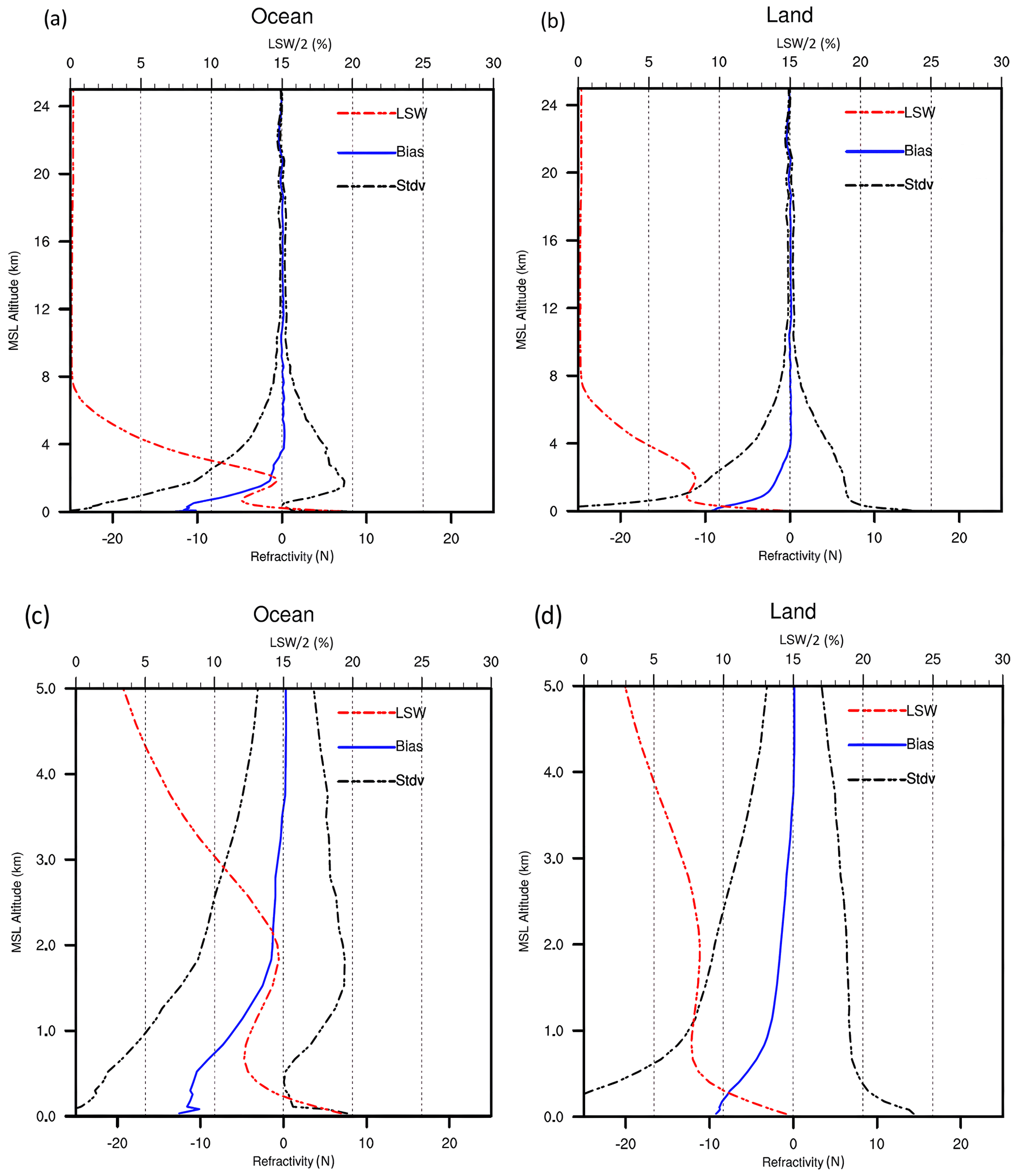
Figure 4Panels (a) and (b) are vertical profiles of the mean and standard deviation of REFB and mean LSW with altitudes up to 25 km over ocean and land, respectively. Panels (c) and (d) are the same as (a) and (b) except are zoomed-in versions below 5 km.
Given the large REFB in the deep troposphere, we focus on the regional variations in REFB averaged below 1.5 km. Figure 5a shows that the averaged value of negative REFB below 1.5 km is largest over the oceanic regions near the western coasts of the South American and African continents. Small negative REFBs appear over the tropical Pacific and over land. There are small positive REFBs over the high-mountain regions. The different behavior of the REFB over ocean and land implies the impact of regional variability and the associated thermodynamic structure in the lower troposphere. As shown in Fig. 5b–d, high LSW occurrence is mainly located over the warm equatorial regions of the Pacific, Atlantic, and Indian oceans. However, not all of the regions with high temperature and moisture coexist with the regions with high LSW. Some exceptional regions can be seen, such as off the coast of southwest Australia and offshore from southwest Africa near the international date line. Figure 5 suggests that although LSW, temperature, and specific humidity have certain cross-relationships, the characteristics of thermodynamic conditions cannot fully explain the distribution of LSW. Therefore, an REFB estimation model that is based on only one variable is not enough to explain REFB.
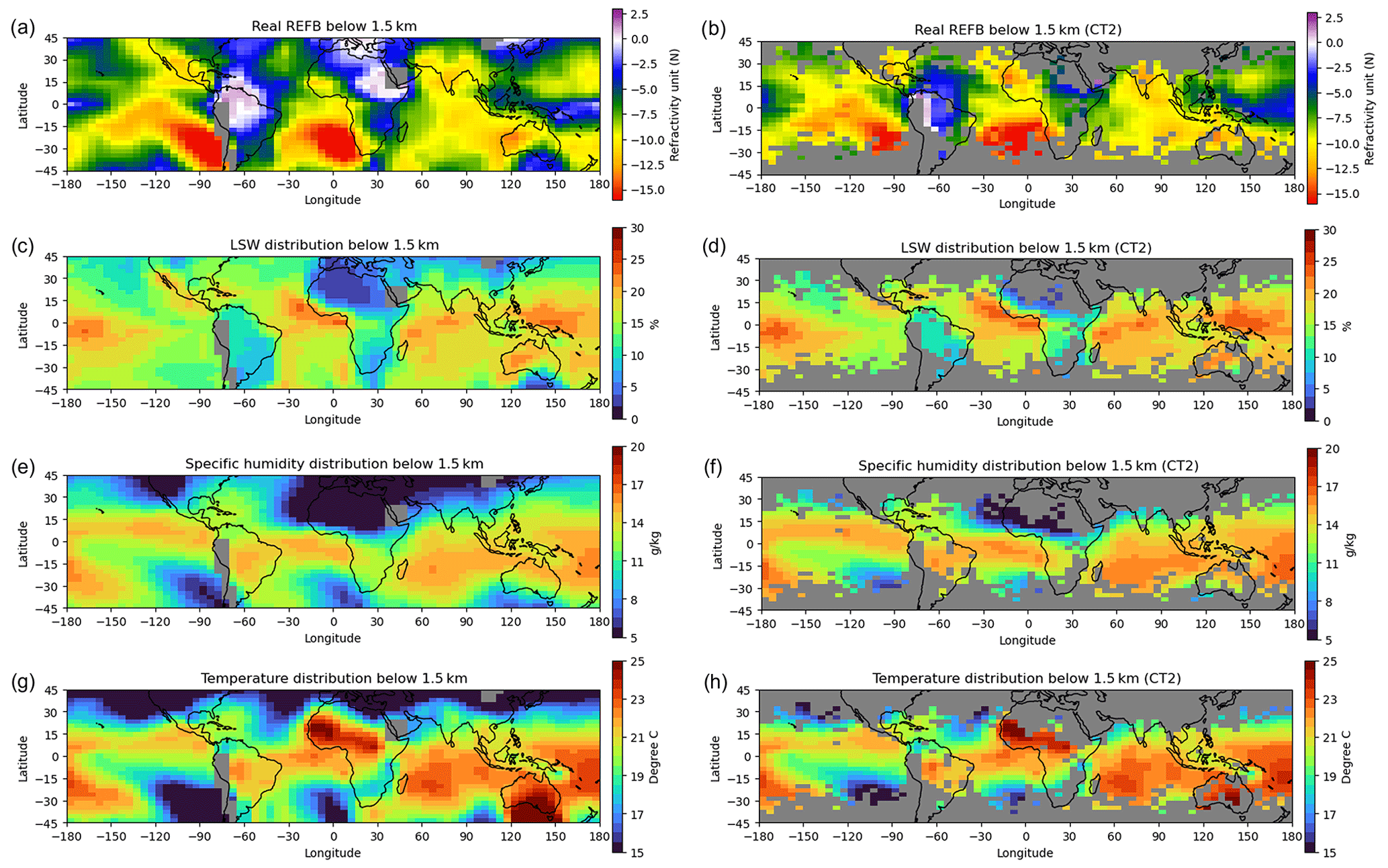
Figure 5Horizontal distribution of (a) REFB (N units), (c) LSW (%), (e) specific humidity (g kg−1), and (g) temperature (°C) during the study period. The values of REFB, LSW, specific humidity, and temperature are averages over the lowest 1.5 km a.m.s.l. of the atmosphere. Panels (b), (d), (f), and (h) are the same as (a), (c), (e), and (g), but they are calculated with the criterion that at least 30 profiles penetrate below 0.5 km in each box.
To further highlight the characteristics of REFB under different conditions, the REFB profiles are grouped according to each profile's LSW, temperature, and specific humidity averaged below 1.5 km for land and ocean (Fig. 6). As Xie (2014) reported, 1.5 km a.m.s.l. is the global mean PBL height calculated from the FS3/C refractivity data. In general, it is evident that the negative REFB increases with increasing LSW below 4 km, as shown in Fig. 3; however, the characteristics are different for land and ocean. Over land, very high LSW does not guarantee the occurrence of a large REFB in the lower troposphere. Moisture and temperature likewise exhibit the same linear relationship with negative REFB in the lower troposphere. However, negative REFBs also tend to occur under conditions of low moisture over the ocean. Figure 6 reveals that the relationship between REFB and LSW and T and Q under 1.5 km is predominantly linear; however, the REFB variations can be further explained by a quadratic relationship with Q. It is noted that REFB at about 10 km increases with increasing LSW, T, and Q over both land and oceans and even becomes weakly positive at high values of LSW, T, and Q averaged below 1.5 km. In particular, RO profiles over land with large LSW below 1.5 km have the largest positive REFB, nearly 8 N unit, aloft. Taking only the RO profiles penetrating 0.5 km will modify the characteristics of Fig. 6 in two ways. First, the REFB below 10 km becomes positive for LSW/2 larger than 28 %. Amplitude of the REFB for cold temperature is larger under 5 km. The former feature is related to the early cutoff height in the tropical occultation over central Africa (Sokolovskiy et al., 2010). Sensitivity tests to address sampling issues will be discussed in Sect. 4.2.
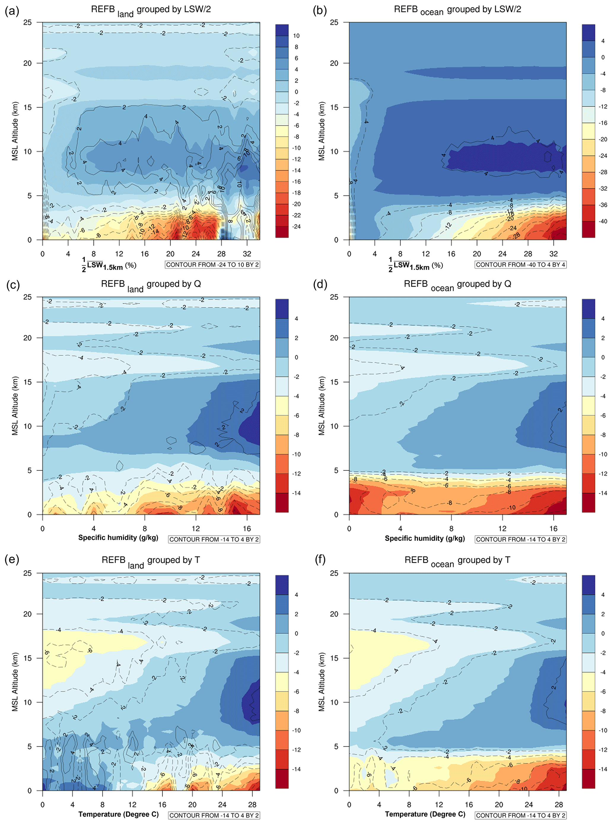
Figure 6Refractivity bias as a function of height and average values over the lowest 1.5 km a.m.s.l. of (a) LSW/2, (c) specific humidity (Q), and (e) temperature (T over land). Panels (b), (d), and (f) are the same as (a), (c), and (e) except over the ocean. The color shading shows the result using the RO profiles penetrating below 1.5 km, while the contour uses the RO profiles penetrating below 0.5 km.
4.1 General performance
In this section, we present the estimation for REFB using the methods introduced in Sect. 2. As mentioned, LSW/2, which represents the retrieval uncertainties in the bending angle and, hence, refractivity uncertainties, is the predictor for the first bias estimation model. T and Q retrieved from FS7/C2 RO data are the predictors for the second estimator. Although the T and Q products retrieved from RO profiles using 1D-Var retrievals may have errors, they still provide valuable information for REFB estimation through the training process, as described in Sect. 2.
Figure 7 shows the relationship between the REFB and LSW/2 averaged below 1.5 km for the Southern Hemisphere (SH) and Northern Hemisphere (NH). REFB is grouped every 2 % of LSW/2, from 0 % to 36 %. The solid and dashed lines show the LSW-based REFB estimates for ocean and land, respectively. Under 1.5 km, the magnitude of the negative REFB as a function of LSW is larger over oceans than over land. Generally, as LSW/2 increases, the REFB becomes more negative below 1.5 km for both land and ocean. Although the relationship is dominated by a linear trend, the quadratic term further improves the regression fitting. As shown in Table 1, the correlations over ocean and land are robust (larger than or close to 0.9) and similar to the training and testing data in SH and NH. Compared to the REFB under the warm and moist conditions of the austral summer in SH, the REFB over NH is weaker, but the relationship between LSW/2 and REFB is still strong over ocean and land, except that the one over land has a somewhat stronger quadratic feature. Given this strong relationship, we expect that the relationship during the boreal summer season will hold as well. However, the relationship between REFB and LSW/2 is not present above 1.5 km, and there is little difference in REFB between land and ocean.
Table 1Correlation coefficients between the mean real and estimated REFBs below 1.5 km over ocean and land in Southern Hemisphere (SH) and Northern Hemisphere (NH).
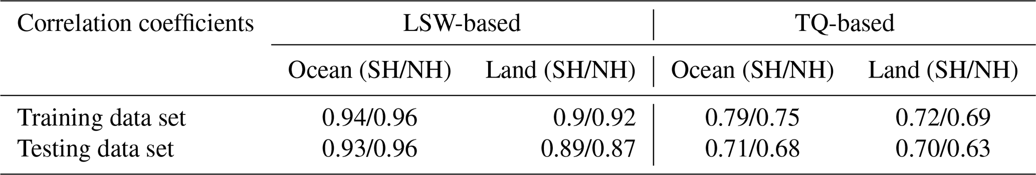
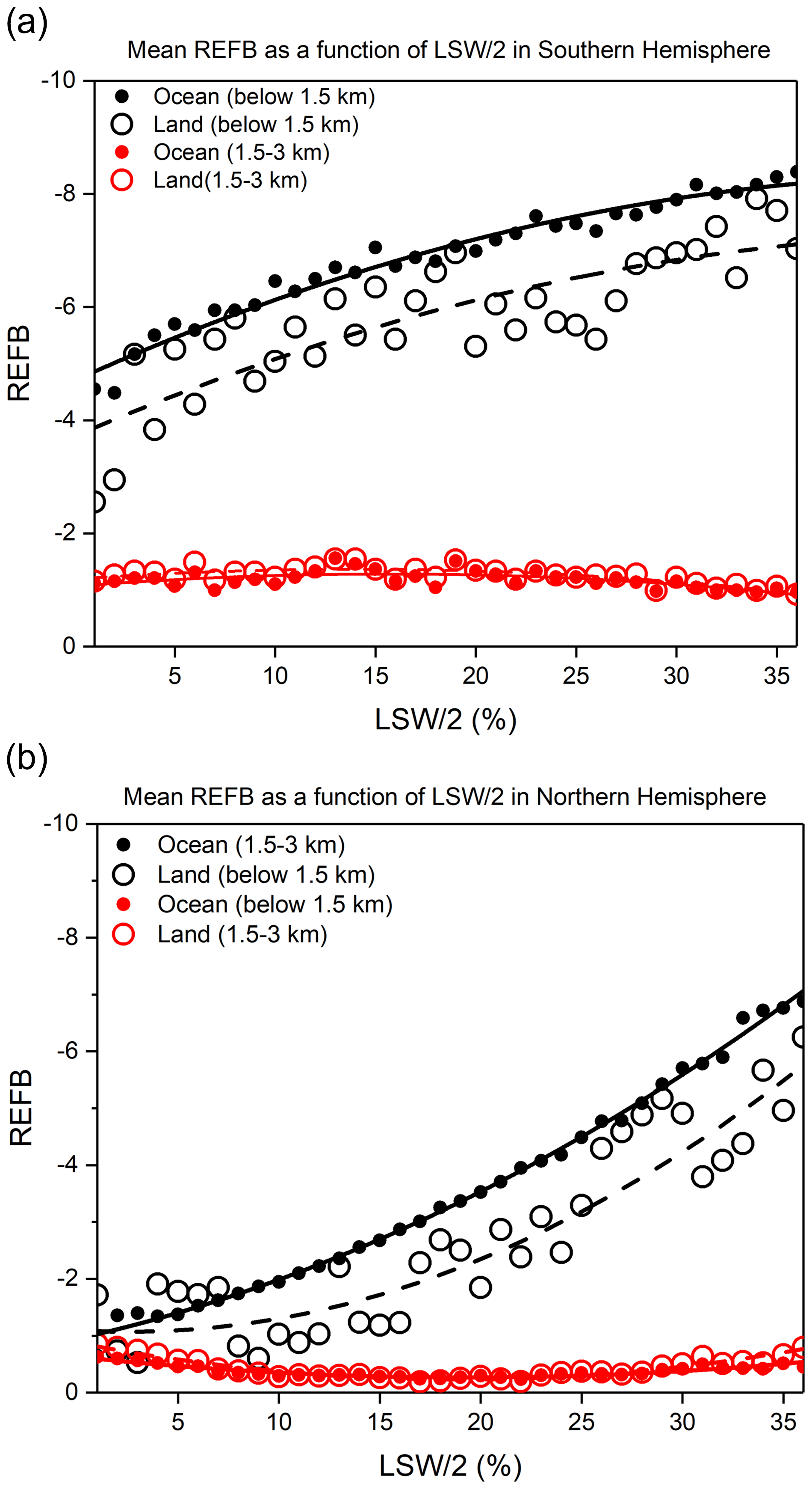
Figure 7The relationship between LSW/2 and REFB. The solid and dashed lines represent the REFB computed from the statistical model for the ocean and land, respectively, as a function of LSW/2 for the Southern Hemisphere (a) and Northern Hemisphere (b). LSW/2 and REFB are averaged below 1.5 km.
Figure 8 shows the result of the second bias estimator, which relates the REFB to the normalized Q (y) and the product of the normalized T and Q (yz) under 1.5 km. The TQ estimation over ocean and land captures the feature where the REFB becomes more negative under moist conditions. Similar to the LSW estimator, the TQ estimator shows a stronger dependence over the ocean. The multivariable regression has correlation coefficients equal to 0.79 and 0.72 for ocean and land in SH, respectively, and 0.75 and 0.69, respectively, in NH. In general, the REFB shows a robust bilinear relationship with y and yz, and the quadratic term (y2) provides further adjustment. With a fixed specific humidity, lower temperature results in larger negative REFB. In Fig. 8a, this result reflects the conditions over the cool sea surface temperature (SST) (Fig. 5a and d) west of the coast of South America and southern Africa. The relationship becomes more linear in NH (Fig. 8a vs. Fig. 8c), i.e., less dependent on the quadratic term of specific humidity. For dryer conditions, the TQ estimator tends to give neutral to positive REFB, especially over land (Fig. 8b and d) where a large amount of data are in the areas with dry conditions and part of them are over the midlatitude continent (Fig. 5c). Given the fixed TQ value (yz = 0.5) in Fig. 8, Fig. 9 shows the strong relationship between REFB and Q. Large negative REFB corresponds to moist conditions, but the negative amplitude is larger over the SH ocean with larger variation. The relationship is more quadratic over ocean than over land and is most linear over the NH land. In Fig. 8, a slightly positive REFB is estimated for very cold and dry conditions over ocean. In Feng et al. (2020), positive REFB is identified in the Bering Sea at high latitudes. While Fig. 8 qualitatively suggests the potential to capture such positive REFB over high latitudes, whether the regional-dependent TQ estimator can be adequately applied to estimate REFB in the polar or high-latitude regions is still an open question since the FS7/C2 data and RO data used in this study are mostly distributed in the tropical to subtropical regions.
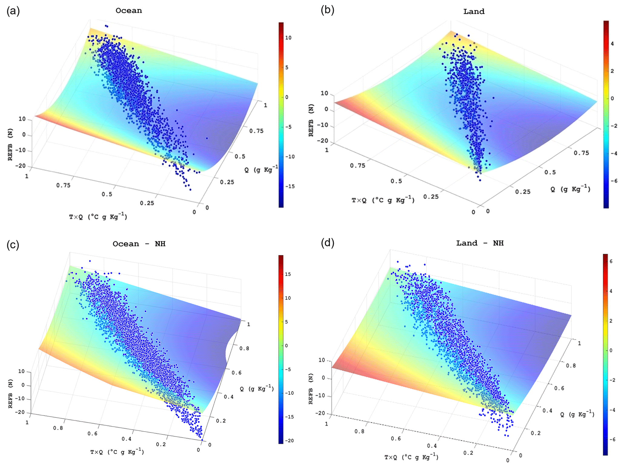
Figure 8The relationships between REFB, normalized specific humidity, the product of normalized temperature, and normalized specific humidity of (a) oceans and (b) land in the Southern Hemisphere. The scatters are the averaged values of each profile below the lowest 1.5 km a.m.s.l. The surfaces show the model computed from a statistical model (Eq. 3) as the function of normalized specific humidity and product of normalized temperature and humidity. Panels (c) and (d) are the same as (a) and (b) but for the Northern Hemisphere (NH).
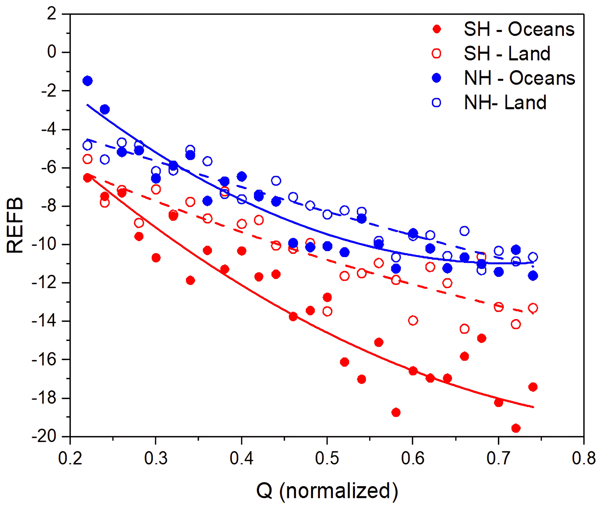
Figure 9The relationship between REFB and normalized Q given a condition of normalized TQ = 0.5.
Figures 7 and 8 confirm that models with LSW/2 or TQ as predictors can estimate the REFB under 1.5 km, but there are different sensitivities for ocean and land. In the next step, we further apply these regression methods using the data in 5° longitude × 3° latitude boxes from 45° N to 45° S to construct the region-dependent bias estimation model.
Figure 10 shows the horizontal distribution of the mean real and estimated REFBs with the training and testing data. Notably, there are some differences between the training and testing data (Fig. 10a vs. Fig. 10b), such as the large REFB off the western coast of South America and off the coast of Australia. In comparison to the real REFB distribution (Fig. 10a), the LSW-based REFB (Fig. 10c) captures the general pattern with larger biases over ocean and lower biases over land in both the training data and testing data. However, the LSW-based REFB is less capable of capturing the large bias over the subtropical oceans off the west coasts of South America, southern Africa, and Australia. Those are expected to be the oceans that have a cold SST, where ducting commonly occurs due to the frequent occurrence of inversion layers on top of the cool sea surface. Although the LSW-based REFB can also represent a portion of the negative REFB in these regions in general, it is obvious that the values are underestimated there. The LSW-based estimation exhibits good performance in estimating the negative REFB in the Indian Ocean, where the pattern and magnitude of the estimated REFB are close to those of the real REFB. In contrast to the LSW-based REFB, the TQ-based REFB represents the large negative REFB in the high-ducting-occurrence regions well. Although the magnitude of the N-REFB off the coasts of South America and southern Africa is still underestimated, the pattern and amplitude of the negative REFB are much better represented in comparison with the LSW-based estimation.
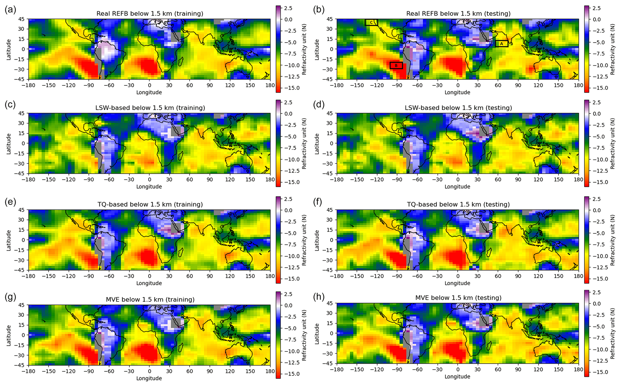
Figure 10Horizontal distribution of refractivity bias and different estimated refractivity biases. The boxes denoted A and B in (b) are the example boxes used in Figs. 12 and 13, respectively. All variables used to construct this figure are averaged below 1.5 km. Area A is in the region of 0–10° N, 55–75° E; area B is in the region of 20–30° S, 85–105° W; and area C is in the region of 35–45° S, 120–135° W.
The TQ-based estimation (Fig. 10e and f) captures the low bias pattern well, such as the tropical western Pacific, western South America, and Africa, while the LSW-based estimation overestimates the negative bias. The similar pattern between the real and TQ-based estimated REFBs can be explained by the following two reasons. The first reason is the ability to capture SST characteristics. For example, cold SST regions can result in a cool, low-moisture near-surface atmosphere (Fig. 5c and d) and can impact the boundary layer. Second, the bias in the RO refractivity profiles will be translated to the 1D-Var T and Q retrievals.
The final method, the MVE, combines the LSW and TQ estimations. As described in Sect. 2, the MVE derives the optimal combination by considering the error correlation between the individual estimations. Notably, the MVE approach requires knowledge of the error covariance matrix between two components (matrix C in Eq. 5). The error correlation of the two REFB estimators is 0.294. A high error correlation indicates a dependency between the two components, and thus there is less benefit from using the MVE method. Although LSW is known to have a relationship to temperature and water vapor, our results indicate that the error correlation between the two estimates is low enough that it is expected that the MVE can extract useful information from both estimations. Compared to the LSW and TQ REFB estimation, the results of the MVE show a pattern closer to the real REFB with both the training data set and the testing data set.
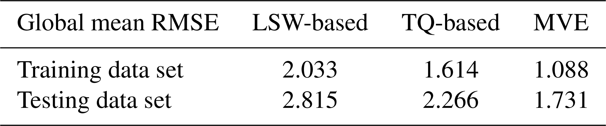
We next show the root mean square error (RMSE) between the real and estimated REFB in each box. Figure 11 shows the contribution of each estimation in estimating bias for land and oceans and reflects the representativeness of the mean REFB shown in Fig. 10. The LSW-based estimation exhibits high RMSE in the cold SST regions and several ocean regions such as the southeastern Atlantic Ocean and southeastern and northwestern Pacific Ocean, while the TQ estimation successfully mitigates this issue. On the other hand, the LSW-based estimation performs better in the tropical Atlantic and Indian oceans. With training and testing data, the large RMSEs in the LSW or TQ estimation over the oceans are largely removed by the MVE method; however, slight degradation is observed over South America and central Africa. With the testing data (Fig. 11b, d, and f), the RMSEs are larger in individual estimations, as expected. In general, the MVE method retains its advantage in the optimal estimation over ocean, with an RMSE smaller than that of either estimation. Table 2 shows the global mean RMSE. The TQ method has a smaller RMSE compared to the LSW estimation. The MVE method further improves the TQ method by 32 % and 23.6 % with the training and testing data, respectively.
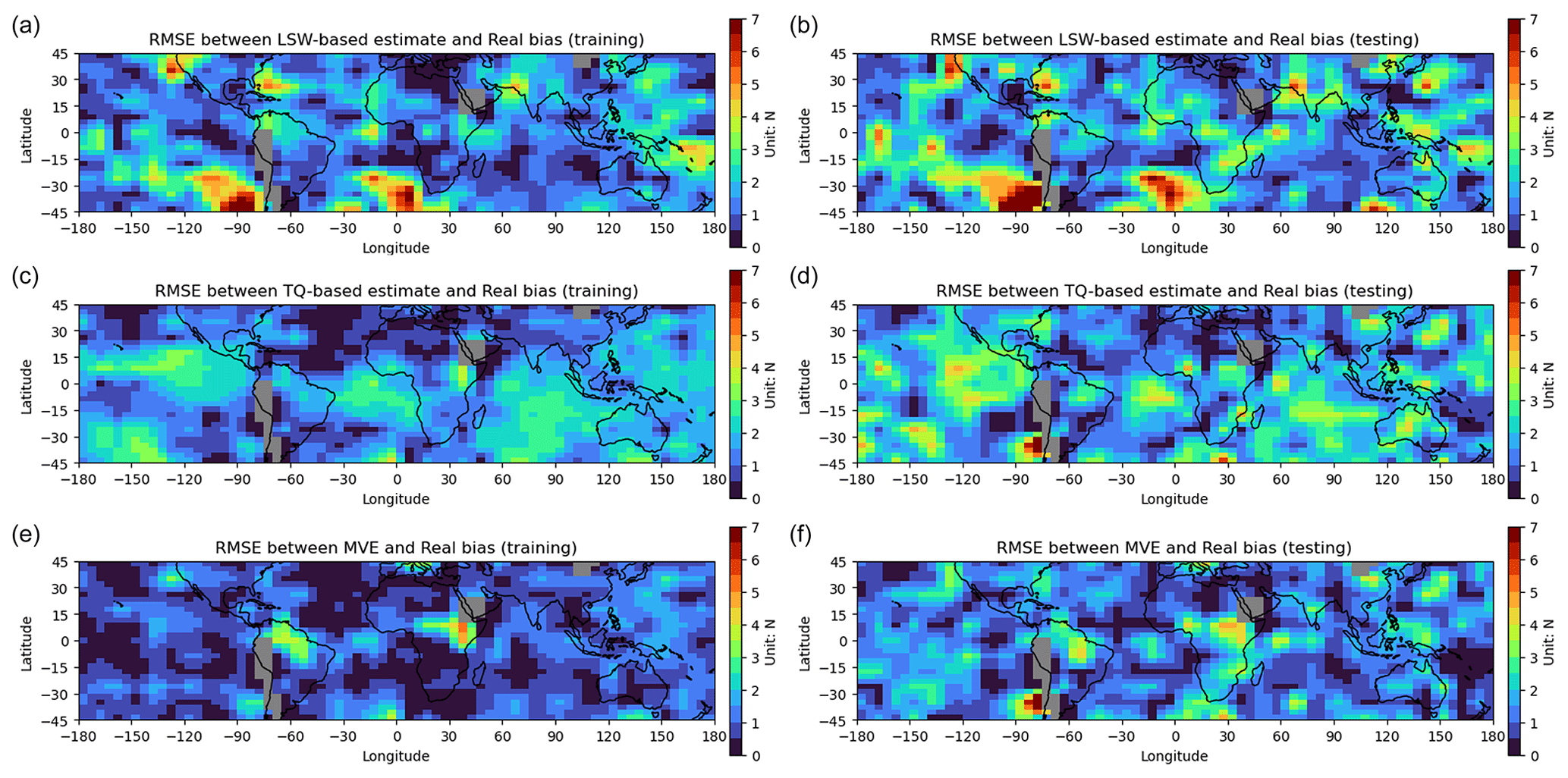
Figure 11Horizontal distribution of RMSE between the real REFB and estimated REFB by different methods with training (a, c, and e) and testing (b, d, and f) data.
Table 2Global mean RMSE of each REFB estimation in comparison to the real REFB below 1.5 km.
However, we also observed that the TQ-based REFB has larger RMSE in the ducting region in the southeast Pacific and Atlantic (Fig. 11e vs. Fig. 11f). This is attributed to an overestimated negative REFB (Fig. 10e vs. Fig. 10f) by the TQ estimator, with much moister near-surface conditions in the testing data than that in the training data. The overestimation of the testing data in the ducting regions suggests that more data are required to train a statistical model applicable to a broader range of temperature and moisture requirements.
4.2 Sensitivity experiments
This subsection discusses the sensitivity of the REFB estimation to the penetration rate of the RO profiles and investigates the impact of sampling error on constructing the LSW-based and TQ-based estimators. Two sets of sensitivities are designed. For the first sensitivity set, it is required that at least 30 RO profiles penetrate a certain level in each box. For the second sensitivity set, the REFB estimators are obtained for RO data from different levels.
Figure 12 shows the REFB estimation with the testing data using different criteria of the penetration rate. The estimators are obtained when there are at least 30 profiles whose minimum level is smaller than 1.5 or 0.5 km. The criteria are referred to as CT1 and CT2 in Fig. 12. As the criterion becomes more stringent, more samples in the tropics are rejected and insufficient samples are available in the core of the ducting regions and in areas with latitudes higher than 30°. For boxes with sufficient samples with the CT2 criterion, the patterns of REFB, LSW, T, and Q (Fig. 5b, d, f, and h) are very similar to the ones with an eased standard criterion, but their amplitudes are generally higher. Nevertheless, the real REFB in Fig. 12a and b is very similar to that in Fig. 10b using an eased criterion for the sample number. This similarity is due to fact that the amount of data between 0.5 and 1.5 km is much more than that below 0.5 km (Fig. 2b). However, the real REFB with CT2 is larger in the southern Pacific and Atlantic. This reflects that the REFB quickly increases near the surface (Fig. 3a), which can be emphasized after the RO profiles with early termination are removed. The LSW-based REFB with strict criteria also captures the general pattern of real REFB, while the TQ-based REFB captures the large negative REFB in the ducting regions well. The REFB estimation using the CT2 criterion still shows good ability in the regions where the real REFBs show some differences between the CT2 and standard criteria, such as the central and northwestern Pacific. This good performance is attributed to the fact that the region-dependent regression models can adapt to the changes in the training data in boxes.
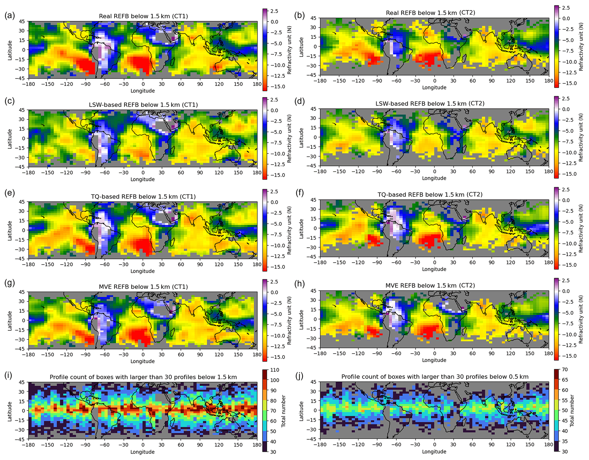
Figure 12The same as Fig. 10, but the calculation was done for RO data with different criteria (CT1 and CT2) for sample selection. CT1 requires that at least 30 RO profiles penetrate below 1.5 km in each box, and CT2 is the same as CT1 except that the profiles penetrate below 0.5 km. Panels (i) and (j) are the horizontal distribution of the profile count with criteria CT1 and CT2, respectively.
Based on the results in Fig. 12, we separate the REFB estimation into different vertical levels: below 0.5 and between 0.5 and 1.5 km (Fig. 13). Comparing Fig. 13a with Fig. 13b, the real REFB below 0.5 km is generally larger than that between 0.5 and 1.5 km, except for the western Pacific and the ducting regions west of South America and southern Africa. Below 0.5 km, the penetration rate declines quickly, reducing the sample size. Nevertheless, it is shown that both REFB estimators perform well in estimating the REFB as well and in particular that the TQ estimator is good at capturing the large REFB. Both estimators can even capture the large negative REFB in the central southern Pacific and southern India, and the MVE REFB improves the TQ-based REFB in the central Pacific (150° W to 150° E). However, the TQ estimator provides positive REFB estimation in the cold and dry conditions north of Africa, while a weak negative value is exhibited in the real REFB. While the TQ estimator is very sensitive to the amplitude of temperature and moisture, we emphasize that the regression model may not be reliable with a limited sampling size in midlatitude regions. Results of the REFB estimation between 0.5 and 1.5 km are very similar to Fig. 10. This again confirms that the REFB shown in Fig. 10 is dominated by the data between 0.5 and 1.5 km. Nevertheless, it is important that both REFB estimators can reflect not only the general characteristics but also the differences at different vertical levels.
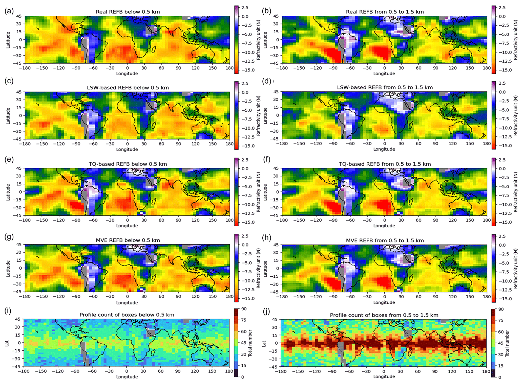
Figure 13The same as Fig. 10, but the calculation was done for RO data from different levels. The left column uses the data below 0.5 km and the right column uses the data between 0.5 and 1.5 km. Panels (i) and (j) are the horizontal distribution of the profile count below 0.5 km and between 0.5 and 1.5 km, respectively.
4.3 Estimating vertical profiles of refractivity bias
This section examines the performance of the REFB estimation methods and whether they can be used for estimating the vertical profiles of REFB. The following three areas (indicated in Fig. 10b) with different REFB characteristics are selected as examples: area A is in the region of 0–10° N, 55–75° E; area B is in the region of 20–30° S, 85–105° W; and area C is in the region of 35–45° S, 120–135° W. For each area, the estimated REFB at different levels is derived using the estimation methods defined in the previous section. Figure 14a–c shows the mean of the real and estimated REFB profiles in three areas with the testing data. We note that the results of the training and testing data are very similar. In area A, the mean negative REFB is large at the surface but gradually reverses to a positive bias at 3 to 5 km. In this case, the air below 2 km is very warm and moist over the Indian Ocean (Fig. 14d). The highly humid conditions give a large LSW (Fig. 5b and c), and thus, the LSW method is able to estimate bias in this circumstance, while the TQ method overestimates the negative REFB. In contrast, area B shows different patterns (Fig. 14b): the real negative REFB is even larger (−17 N units) at the surface, and the negative bias at 2 km is still large compared to that in area A. As shown in Fig. 14d, this characteristic is associated with typical conditions for ducting, such as the existence of an inversion layer at 2 km over the cold SST region accompanied with a large vertical moisture gradient. While the LSW-based estimation underestimates the negative REFB, with the existence of the inversion layers this can be captured by the TQ-based estimation. Nevertheless, the MVE method is always much closer to the real REFB. In Fig. 14b, area B shows improvement in the MVE compared to the TQ-based estimation, while a large RMSE remained in area B with the MVE method in Fig. 11f. It should be noted that Fig. 11 is calculated based on the difference between the real REFB and estimated REFB of each profile “averaged” below 1.5 km, where Fig. 14 groups the profiles with an interval of 500 m. Therefore, the overestimation in the REFB below 1 km with the TQ-based estimator is alleviated with the average data used to construct Fig. 11.
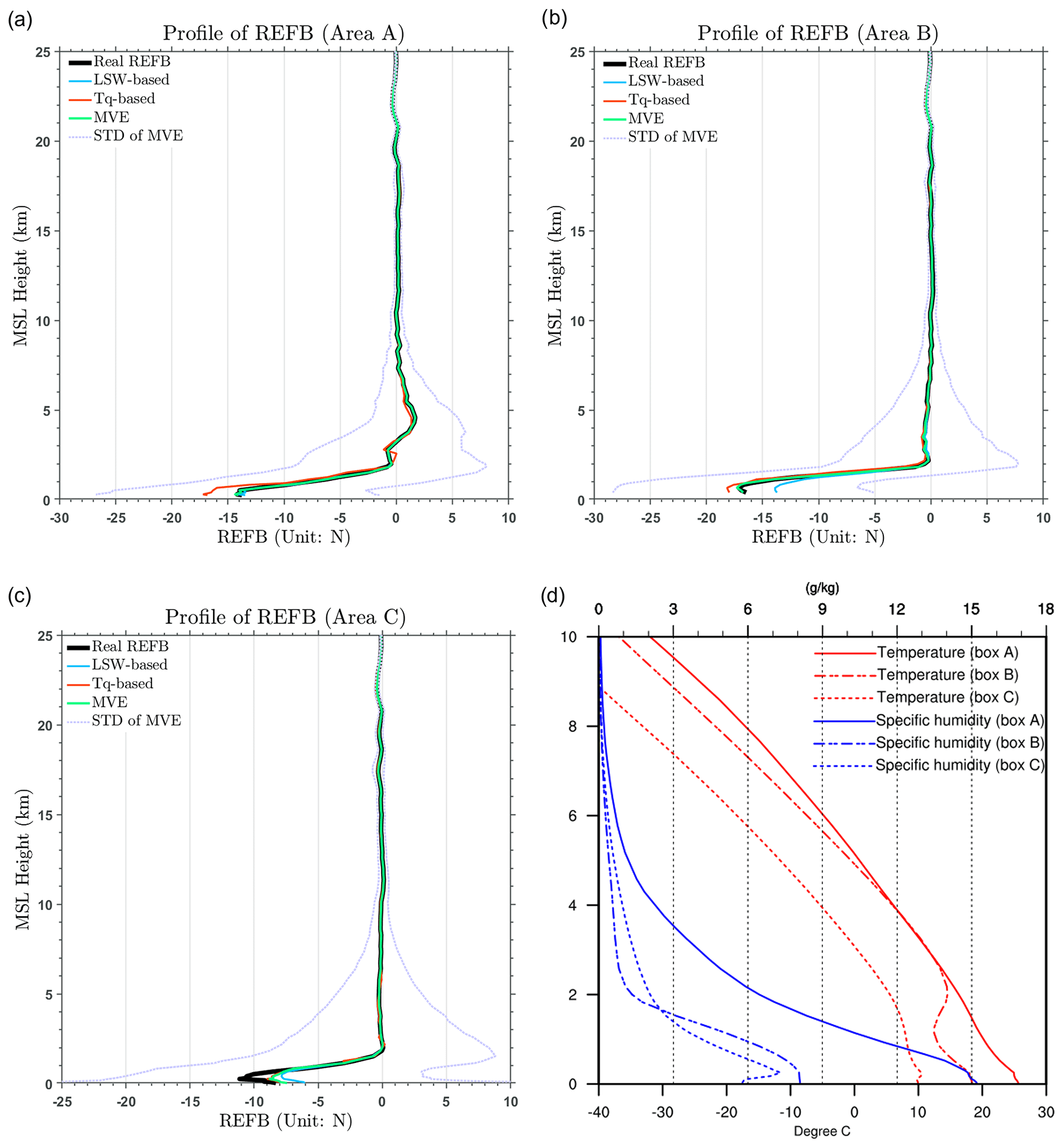
Figure 14Profiles of refractivity bias (real and estimates) for three different areas selected in Fig. 10b. Boxes A, B, and C are in 0–10° N, 55–75° E; 20–30° S, 85–105° W; and 35–45° S, 120–135° W. (d) Profiles of temperature (red lines) and specific humidity (blue lines) averaged for areas A (solid lines), B (long-dashed lines), and C (short-dashed lines) shown in Fig. 10b.
For the box located off the coast of North America with midlatitude cold and dry conditions (Fig. 14c), both estimators capture the general pattern of the vertical distribution of REFB, but the amplitude below 1 km is smaller than the real REFB. Nevertheless, the TQ-based REFB is much better represented compared to the one from the LSW estimator. Figure 14 suggests that both estimators can be applied to estimate the vertical variations in REFB in different regions. However, sample issues may be encountered in midlatitude regions as discussed in Sect. 4.2.
This study investigates the characteristics of the refractivity bias (REFB) of FS7/C2 and its sensitivities to RO measurement uncertainty (LSW) and thermodynamic conditions (temperature and moisture). Two bias estimation models are constructed based on polynomial regression with the LSW, and temperature and specific humidity are used as predictors in each estimation. The study period is December 2019–February 2020, with the ERA5 reanalysis data taken as the reference.
Similar to previous studies, the low-level FS7/C2 RO refractivity data of the study period contain significant biases when compared with ERA5 data. In general, the REFB below 1.5 km is negatively proportional to LSW and exhibits a stronger dependency over ocean than over land. Additionally, REFB in the PBL has a strong dependence on low-level temperature and moisture. While the majority of the Pacific and Indian oceans with warm SSTs has significant negative REFBs, the largest negative REFB regions are near the cold SST regions off the western coasts of South America and southern Africa. Small and even positive REFBs are observed over South America and southern Africa.
Two REFB estimation models based on the polynomial regression approach are first applied to construct the region-dependent mean REFB below 1.5 km. One estimation model uses a quadratic function of LSW. The other uses the multivariable polynomial regression with temperature and specific humidity (TQ) as predictors, and the moisture variable becomes emphasized after optimization. The estimation models are then applied to 72 × 30 boxes from 45° N to 45° S. The minimum error variance (MVE) method is used to combine two REFB estimations. The results show that the bias estimation models with either LSW or TQ have their own advantages in estimating REFB. The LSW-based model shows the ability to capture the general pattern of the negative REFB, but the amplitude is significantly underestimated in the ducting areas. The TQ-based model has great performance in representing the pattern and amplitude of REFB, particularly the large negative REFB in the ducting areas and small REFB over most land regions. While the relationship between REFB and LSW below 1.5 km is very strong in a global sense, the TQ-based REFB shows its advantage in capturing the regional characteristics. The MVE estimation successfully adopts the advantages from both the LSW estimation and the TQ estimation and has the smallest RMSE, particularly over ocean.
Results of sensitivity tests show that the estimators at midlatitude could be affected by the sampling issue since requiring profiles to penetrate 0.5 km means that we cannot obtain sufficient samples to construct the regression models. With the 3 months of data, the REFB estimation in tropical to subtropical regions remains similar to the RO profiles penetrating below 1.5 or below 0.5 km given that the amount of RO data between 0.5 and 1.5 km dominates. Nevertheless, both the LSW and TQ estimations can capture the characteristics of REFB when the RO data are separated to below 0.5 and between 0.5 and 1.5 km. Such an ability allows the three REFB estimation models to be applied to reconstruct the REFB vertical profiles for regions with distinct thermodynamic conditions in the deep troposphere. Both the LSW and TQ estimations can represent the vertical gradient of the mean REFB well, and the MVE estimation gives an estimated REFB profile closest to the real REFB with a probability distribution similar to the distribution of the real REFB.
We should note some of the limitations of these REFB models. The temperature and moisture from the ERA5 reanalysis may have a bias. In addition, REFB may have more characteristics regarding smaller scales spatiotemporally. We should also emphasize that the FS7/C2 RO data are mainly located in the tropical to subtropical regions. Therefore, we need more data to justify whether the regression-based bias estimation is applicable in high-latitude regions. Finally, predictors used in the statistical models may not be enough to capture all attributions of REFB. For future work, bias estimation models will be constructed at higher resolutions with more RO profiles collected from the current FS7/C2 or other operational and commercial GNSS RO satellites.
The code for the bias estimators used in this study is available on Zenodo at https://doi.org/10.5281/zenodo.8021390 (jiajia170801, 2023). The RO data were obtained from the Taiwan Analysis Center for COSMIC (TACC) at https://tacc.cwb.gov.tw/data-service/fs7rt_tdpc/ (Central Weather Bureau (Taiwan) and Taiwan Space Agency (TASA), 2020). The ECMWF reanalysis v5 (ERA5) data were obtained from the Copernicus Climate Change Service (C3S) at https://doi.org/10.24381/cds.bd0915c6 (Hersbach et al., 2023).
SY was in charge of the conceptualization of this study. SY and GP prepared the paper with contributions from all co-authors. GP constructed the packages of bias estimation. SY and GP analyzed the data. SY and GP wrote the manuscript draft; CC, SC, and CH reviewed and edited the paper.
The contact author has declared that none of the authors has any competing interests.
Publisher's note: Copernicus Publications remains neutral with regard to jurisdictional claims made in the text, published maps, institutional affiliations, or any other geographical representation in this paper. While Copernicus Publications makes every effort to include appropriate place names, the final responsibility lies with the authors.
The authors greatly appreciate Richard Anthes and the anonymous reviewer for insightful comments and suggestions for improving the paper.
This research has been supported by the Taiwan National Science and Technology Council (grant nos. NSTC-111-2121-M-008-001 and NSTC-111-2111-M-008-030) and the Taiwan Space Agency (grant no. TASA-S-110316).
This paper was edited by Peter Alexander and reviewed by Richard Anthes and one anonymous referee.
Anthes, R., Sjoberg, J., Feng, X., and Syndergaard, S.: Comparison of COSMIC and COSMIC-2 Radio Occultation Refractivity and Bending Angle Uncertainties in August 2006 and 2021, Atmosphere, 13, 790, https://doi.org/10.3390/atmos13050790, 2022.
Ao, C. O., Meehan, T. K., Hajj, G. A., Mannucci, A. J., and Beyerle, G.: Lower troposphere refractivity bias in GPS occultation retrievals, J. Geophys. Res.-Atmos., 108, 4577, https://doi.org/10.1029/2002JD003216, 2003.
Bowler, N. E.: An assessment of GNSS radio occultation data produced by Spire, Q. J. Roy. Meteor. Soc., 146, 3772–3788, https://doi.org/10.1002/qj.3872, 2020a.
Bowler, N. E.: Revised GNSS-RO observation uncertainties in the Met Office NWP system, Q. J. Roy. Meteor. Soc., 146, 2274–2296, https://doi.org/10.1002/qj.3791, 2020b.
Central Weather Bureau (Taiwan) and Taiwan Space Agency (TASA): FS-7 Taiwan Data Processing Center (TDPC) Realtime, TACC [data set], https://tacc.cwb.gov.tw/data-service/fs7rt_tdpc/, last access: 24 June 2020.
Chang, C.-C. and Yang, S.-C.: Impact of assimilating Formosat-7/COSMIC-II GNSS radio occultation data on heavy rainfall prediction in Taiwan, Terr. Atmos. Ocean. Sci., 33, 7, https://doi.org/10.1007/s44195-022-00004-4, 2022.
Chen, S.-Y., Kuo, Y.-H., and Huang, C.-Y.: The Impact of GPS RO Data on the Prediction of Tropical Cyclogenesis Using a Nonlocal Observation Operator: An Initial Assessment, Mon. Weather Rev., 148, 2701–2717, https://doi.org/10.1175/mwr-d-19-0286.1, 2020.
Chen, S.-Y., Shih, C.-P., Huang, C.-Y., and Teng, W.-H.: An Impact Study of GNSS RO Data on the Prediction of Typhoon Nepartak (2016) Using a Multi-resolution Global Model with 3D-Hybrid Data Assimilation, Weather Forecast., 36, 957–977, https://doi.org/10.1175/waf-d-20-0175.1, 2021a.
Chen, S.-Y., Nguyen, T.-C., and Huang, C.-Y.: Impact of Radio Occultation Data on the Prediction of Typhoon Haishen (2020) with WRFDA Hybrid Assimilation, Atmosphere, 12, 1397, https://doi.org/10.3390/atmos12111397, 2021b.
Chen, S.-Y., Liu, C.-Y., Huang, C.-Y., Hsu, S.-C., Li, H.-W., Lin, P.-H., Cheng, J.-P., and Huang, C.-Y.: An Analysis Study of FORMOSAT-7/COSMIC-2 Radio Occultation Data in the Troposphere, Remote Sens.-Basel, 13, 717, https://doi.org/10.3390/rs13040717, 2021c.
Chen, Y.-J., Hong, J.-S., and Chen, W.-J.: Impact of Assimilating FORMOSAT-7/COSMIC-2 Radio Occultation Data on Typhoon Prediction Using a Regional Model, Atmosphere, 13, 1879, https://doi.org/10.3390/atmos13111879, 2022.
Clarizia, M. P., Ruf, C. S., Jales, P., and Gommenginger, C.: Spaceborne GNSS-R Minimum Variance Wind Speed Estimator, IEEE. T. Geosci. Remote, 52, 6829–6843, https://doi.org/10.1109/tgrs.2014.2303831, 2014.
Cucurull, L., Derber, J. C., Treadon, R., and Purser, R. J.: Assimilation of Global Positioning System Radio Occultation Observations into NCEP's Global Data Assimilation System, Mon. Weather Rev., 135, 3174–3193, https://doi.org/10.1175/mwr3461.1, 2007.
Cucurull, L., Li, R., and Peevey, T. R.: Assessment of Radio Occultation Observations from the COSMIC-2 Mission with a Simplified Observing System Simulation Experiment Configuration, Mon. Weather Rev., 145, 3581–3597, https://doi.org/10.1175/mwr-d-16-0475.1, 2017.
Eyre, J. R.: An introduction to GPS radio occultation and its use in numerical weather prediction, Proceedings of the ECMWF GRAS SAF workshop on applications of GPS radio occultation measurements, Shinfield Park, Reading, 16–18 June 2008.
Feng, X., Xie, F., Ao, C. O., and Anthes, R. A.: Ducting and Biases of GPS Radio Occultation Bending Angle and Refractivity in the Moist Lower Troposphere, J. Atmos. Ocean. Tech., 37, 1013–1025, https://doi.org/10.1175/jtech-d-19-0206.1, 2020.
Gorbunov, M. E.: Canonical transform method for processing radio occultation data in the lower troposphere, Radio Sci., 37, 9-1–9-10, https://doi.org/10.1029/2000rs002592, 2002.
Gorbunov, M. E., Lauritsen, K. B., Rhodin, A., Tomassini, M., and Kornblueh, L.: Radio holographic filtering, error estimation, and quality control of radio occultation data, J. Geophys. Res.-Atmos., 111, D10105, https://doi.org/10.1029/2005jd006427, 2006.
Gorbunov, M. E., Vorob'ev, V. V., and Lauritsen, K. B.: Fluctuations of refractivity as a systematic error source in radio occultations, Radio Sci., 50, 656–669, https://doi.org/10.1002/2014rs005639, 2015.
Healy, S. B.: Forecast impact experiment with a constellation of GPS radio occultation receivers, Atmos. Sci. Lett., 9, 111–118, https://doi.org/10.1002/asl.169, 2008.
Healy, S.: Assimilation in the upper-troposphere and lower-stratosphere: The role of GPS radio occultation, Seminar on Use of Satellite Observations in Numerical Weather Prediction, Shinfield Park, Reading, 8–12 September 2014.
Hersbach, H., Bell, B., Berrisford, P., Biavati, G., Horányi, A., Muñoz Sabater, J., Nicolas, J., Peubey, C., Radu, R., Rozum, I., Schepers, D., Simmons, A., Soci, C., Dee, D., and Thépaut, J.-N.: ERA5 hourly data on pressure levels from 1940 to present, Copernicus Climate Change Service (C3S) Climate Data Store (CDS) [data set], https://doi.org/10.24381/cds.bd0915c6, 2023.
Jensen, A. S., Lohmann, M. S., Benzon, H.-H., and Nielsen, A. S.: Full Spectrum Inversion of radio occultation signals, Radio Sci., 38, 1040, https://doi.org/10.1029/2002rs002763, 2003.
Jensen, A. S., Lohmann, M. S., Nielsen, A. S., and Benzon, H.-H.: Geometrical optics phase matching of radio occultation signals, Radio Sci., 39, RS3009, https://doi.org/10.1029/2003rs002899, 2004.
jiajia170801: jiajia170801/bias_estimation_paper: First Publicity 2023/06/10 (Papers), Zenodo [code], https://doi.org/10.5281/zenodo.8021390, 2023.
Kuo, Y.-H., Wee, T.-K., Sokolovskiy, S., Rocken, C., Schreiner, W., Hunt, D., and Anthes, R. A.: J. Meteorol. Soc. Jpn., 82, 507–531, https://doi.org/10.2151/jmsj.2004.507, 2004.
Lien, G.-Y., Lin, C.-H., Huang, Z.-M., Teng, W.-H., Chen, J.-H., Lin, C.-C., Ho, H.-H., Huang, J.-Y., Hong, J.-S., Cheng, C.-P., and Huang, C.-Y.: Assimilation Impact of Early FORMOSAT-7/COSMIC-2 GNSS Radio Occultation Data with Taiwan's CWB Global Forecast System, Mon. Weather Rev., https://doi.org/10.1175/mwr-d-20-0267.1, 2021.
Lien, T. Y., Yeh, T. K., Wang, C. S., Xu, Y., Jiang, N., and Yang, S. C.: Accuracy verification of the precipitable water vapor derived from COSMIC-2 radio occultation using ground-based GNSS, Adv. Space Res., 73, 4597–4607, https://doi.org/10.1016/j.asr.2024.01.041, 2024.
Liu, H., Kuo, Y.-H., Sokolovskiy, S., Zou, X., Zeng, Z., Hsiao, L.-F., and Ruston, B. C.: A Quality Control Procedure Based on Bending Angle Measurement Uncertainty for Radio Occultation Data Assimilation in the Tropical Lower Troposphere, J. Atmos. Ocean. Tech., 35, 2117–2131, https://doi.org/10.1175/jtech-d-17-0224.1, 2018.
Lopez, P.: A 5-yr 40-km-Resolution Global Climatology of Superrefraction for Ground-Based Weather Radars, J. Appl. Meteorol. Clim., 48, 89110, https://doi.org/10.1175/2008JAMC1961.1, 2009.
Rennie, M. P.: The impact of GPS radio occultation assimilation at the Met Office, Q. J. Roy. Meteor. Soc., 136, 116–131, https://doi.org/10.1002/qj.521, 2010.
Rocken, C., Anthes, R., Exner, M., Hunt, D., Sokolovskiy, S., Ware, R., Gorbunov, M., Schreiner, W., Feng, D., Herman, B., Kuo, Y. H., and Zou, X.: Analysis and validation of GPS/MET data in the neutral atmosphere, J. Geophys. Res.-Atmos., 102, 29849–29866, https://doi.org/10.1029/97jd02400, 1997.
Schreiner, W., Sokolovskiy, S., Hunt, D., Rocken, C., and Kuo, Y.-H.: Analysis of GPS radio occultation data from the FORMOSAT-3/COSMIC and Metop/GRAS missions at CDAAC, Atmos. Meas. Tech., 4, 2255–2272, https://doi.org/10.5194/amt-4-2255-2011, 2011.
Schreiner, W. S., Weiss, J. P., Anthes, R. A., Braun, J., Chu, V., Fong, J., Hunt, D., Kuo, Y. H., Meehan, T., Serafino, W., Sjoberg, J., Sokolovskiy, S., Talaat, E., Wee, T. K., and Zeng, Z.: COSMIC-2 Radio Occultation Constellation: First Results, Geophys. Res. Lett., 47, e2019GL086841, https://doi.org/10.1029/2019gl086841, 2020.
Sirmans, D. and Bumgarner B.: Numerical Comparison of Five Mean Frequency Estimators, J. Appl. Meteorol. Clim., 14, 9911003, https://doi.org/10.1175/1520-0450(1975)014<0991:NCOFMF>2.0.CO;2, 1975.
Sjoberg, J., Anthes, R. A., and Zhang, H.: Estimating individual radio occultation uncertainties using the observations and environmental parameters, J. Atmos. Ocean Tech., 40, 1461–1474, 2023.
Sokolovskiy, S. V.: Modeling and inverting radio occultation signals in the moist troposphere, Radio Sci., 36, 441–458, https://doi.org/10.1029/1999RS002273, 2001.
Sokolovskiy, S.: Effect of superrefraction on inversions of radio occultation signals in the lower troposphere, Radio Sci., 38, 1058, https://doi.org/10.1029/2002rs002728, 2003.
Sokolovskiy, S., Rocken, C., Schreiner, W., and Hunt, D.: On the uncertainty of radio occultation inversions in the lower troposphere, J. Geophys. Res., 115, D22111, https://doi.org/10.1029/2010jd014058, 2010.
Sokolovskiy, S., Schreiner, W., Zeng, Z., Hunt, D., Lin, Y.-C., and Kuo, Y.-H.: Observation, analysis, and modeling of deep radio occultation signals: Effects of tropospheric ducts and interfering signals, Radio Sci., 49, 954–970, https://doi.org/10.1002/2014RS005436, 2014.
Sokolovskiy, S., Zeng, Z., Hunt, D., Weiss, J.-P., Braun, J., Schreiner, W., Anthes, R., Kuo, Y.-H., Zhang, H., Lenschow, D., and VanHove, T.: Detection of super-refraction at the top of the atmospheric boundary layer from COSMIC-2 radio occultations, J. Atmos. and Ocean Tech., 40, 65–78, https://doi.org/10.1175/JTECH-D-22-0100.1, 2024.
Wang, K.-N., de la Torre Juárez, M., Ao, C. O., and Xie, F.: Correcting negatively biased refractivity below ducts in GNSS radio occultation: an optimal estimation approach towards improving planetary boundary layer (PBL) characterization, Atmos. Meas. Tech., 10, 4761–4776, https://doi.org/10.5194/amt-10-4761-2017, 2017.
Wang, K.-N., Ao, C., and de la Torre Juárez, M.: GNSS-RO Refractivity Bias Correction Under Ducting Layer Using Surface-Reflection Signal, Remote Sens.-Basel, 12, 359, https://doi.org/10.3390/rs12030359, 2020.
Wee, T.-K., Anthes, R. A., Hunt, D. C., Schreiner, W. S., Kuo, Y.-H.: Atmospheric GNSS RO 1D-Var in Use at UCAR: Description and Validation, Remote Sens.-Basel, 14, 5614, https://doi.org/10.3390/rs14215614, 2022.
Xie, F.: Investigation of methods for the determination of the PBL height from RO observations using ECMWF reanalysis data, ROM SAF CDOP-2 Visiting Scientist Report 21, Radio Occultation Meteorology Satellite Application Facility, https://www.romsaf.org (last access: 18 January 2024), 2014.
Xie, F., Syndergaard, S., Kursinski, E. R., and Herman, B. M.: An Approach for Retrieving Marine Boundary Layer Refractivity from GPS Occultation Data in the Presence of Superrefraction, J. Atmos. Ocean. Tech., 23, 1629–1644, https://doi.org/10.1175/JTECH1996.1, 2006.
Xie, F., Wu, D. L., Ao, C. O., Kursinski, E. R., Mannucci, A. J., and Syndergaard, S.: Super-refraction effects on GPS radio occultation refractivity in marine boundary layers, Geophys. Res. Lett., 37, L11805, https://doi.org/10.1029/2010gl043299, 2010.
Yang, J., Wang, Z., Heymsfield, A. J., and French, J. R.: Characteristics of vertical air motion in isolated convective clouds, Atmos. Chem. Phys., 16, 10159–10173, https://doi.org/10.5194/acp-16-10159-2016, 2016.
Yang, S.-C., Chen, S.-H., Chen, S.-Y., Huang, C.-Y., and Chen, C.-S.: Evaluating the Impact of the COSMIC RO Bending Angle Data on Predicting the Heavy Precipitation Episode on 16 June 2008 during SoWMEX-IOP8, Mon. Weather Rev., 142, 4139–4163, https://doi.org/10.1175/mwr-d-13-00275.1, 2014.
Zhang, H., Kuo, Y.-H., and Sokolovskiy, S.: Assimilation of Radio Occultation Data Using Measurement-Based Observation Error Specification: Preliminary Results, Mon. Weather Rev., 151, 589–601, https://doi.org/10.1175/mwr-d-22-0122.1, 2023.