the Creative Commons Attribution 4.0 License.
the Creative Commons Attribution 4.0 License.
 | 05 Jan 2024
Assessing potential indicators of aerosol wet scavenging during long-range transport
Miguel Ricardo A. Hilario
Avelino F. Arellano
Ali Behrangi
Ewan C. Crosbie
Joshua P. DiGangi
Glenn S. Diskin
Michael A. Shook
Luke D. Ziemba
As one of the dominant sinks of aerosol particles, wet scavenging greatly influences aerosol lifetime and interactions with clouds, precipitation, and radiation. However, wet scavenging remains highly uncertain in models, hindering accurate predictions of aerosol spatiotemporal distributions and downstream interactions. In this study, we present a flexible, computationally inexpensive method to identify meteorological variables relevant for estimating wet scavenging using a combination of aircraft, satellite, and reanalysis data augmented by trajectory modeling to account for air mass history. We assess the capabilities of an array of meteorological variables to predict the transport efficiency of black carbon (TEBC) using a combination of nonlinear regression, curve fitting, and k-fold cross-validation. We find that accumulated precipitation along trajectories (APT) – treated as a wet scavenging indicator across multiple studies – does poorly when predicting TEBC. Among different precipitation characteristics (amount, frequency, intensity), precipitation intensity was the most effective at estimating TEBC but required longer trajectories (>48 h) and including only intensely precipitating grid cells. This points to the contribution of intense precipitation to aerosol scavenging and the importance of accounting for air mass history. Predictors that were most able to predict TEBC were related to the distribution of relative humidity (RH) or the frequency of humid conditions along trajectories, suggesting that RH is a more robust way to estimate TEBC than APT. We recommend the following alternatives to APT when estimating aerosol scavenging: (1) the 90th percentile of RH along trajectories, (2) the fraction of hours along trajectories with either water vapor mixing ratios >15 g kg−1 or RH >95 %, and (3) precipitation intensity along trajectories at least 48 h along and filtered for grid cells with precipitation >0.2 mm h−1. Future scavenging parameterizations should consider these meteorological variables along air mass histories. This method can be repeated for different regions to identify region-specific factors influencing wet scavenging.
- Article
(3109 KB) - Full-text XML
-
Supplement
(1287 KB) - BibTeX
- EndNote


Although wet scavenging is one of the dominant removal mechanisms for atmospheric aerosol particles (Seinfeld and Pandis, 2016; Textor et al., 2006), it remains a large source of uncertainty in global-scale models (Watson-Parris et al., 2019; Liu and Matsui, 2021; Moteki et al., 2019; Hodzic et al., 2016). This uncertainty hampers the ability of global-scale models to capture the life cycle (i.e., sources, transformations, and sinks) (Hou et al., 2018), spatial extent (Moteki et al., 2019), and vertical profile (Watson-Parris et al., 2019; Liu and Matsui, 2021; Frey et al., 2021; Kipling et al., 2016) of aerosol particles. Inaccurate representations of these aerosol features contribute to uncertainties in estimates of aerosol radiative effects (Samset et al., 2013; Marinescu et al., 2017) and aerosol loadings over climate-sensitive regions (Liu and Matsui, 2021; Mahmood et al., 2016; Shen et al., 2017), with further implications for the remote sensing of aerosol abundance downwind of precipitating or cloudy areas. Advancing knowledge of wet scavenging processes can help reduce the largest uncertainty in human forcing of the climate system, which involves aerosol–cloud interactions (e.g., Bellouin et al., 2020).
Wet scavenging occurs either below- or in-cloud. Below-cloud scavenging occurs when aerosol particles are collected by precipitation (Croft et al., 2009) and is most important between the surface and 1 km above ground level (a.g.l.) (Grythe et al., 2017). The efficiency of below-cloud scavenging depends on raindrop size distributions (Wang et al., 2010), aerosol composition (Lu and Fung, 2018; Grythe et al., 2017), the amount of in-cloud condensed water (Luo et al., 2019), and precipitation characteristics (i.e., frequency, intensity, amount, and type). To calculate the fraction of aerosol scavenged below-cloud, models typically rely on an empirically derived below-cloud scavenging coefficient, which is a function of aerosol size (Feng, 2007; Croft et al., 2009) and composition (Lin et al., 2021). Semi-empirical model parameterizations of below-cloud scavenging have been shown to improve simulated surface concentrations (Luo et al., 2019); however, agreement between models and observations is highly sensitive to the specific below-cloud scavenging scheme used (Lu and Fung, 2018). Below-cloud scavenging rates in models also remain significantly underestimated compared to observations (Kim et al., 2021; Ryu and Min, 2022; Xu et al., 2019).
Wang et al. (2010) determined that the below-cloud scavenging coefficient is influenced by (1) raindrop particle collection efficiency, (2) raindrop size distribution, and (3) raindrop terminal velocity. These factors were associated with differences in particle concentrations by a factor of 2 for sub-10 nm particles and a factor of >10 for particles larger than 3 µm; however, their combined uncertainty was insufficient to explain the discrepancy between theoretical and field measurements of the below-cloud scavenging coefficient. Wang et al. (2011) demonstrated that this discrepancy can be largely explained by the vertical turbulence as it determines which particles are subjected to impaction scavenging. This impact was most pronounced for submicron particles under weak precipitation intensities.
Given these uncertainties, Wang et al. (2014a) developed a new semi-empirical, size-resolved parameterization based on an percentile logarithmic power-law relationship between the below-cloud scavenging coefficient and particle size that is applicable to both rain and snow across different particle sizes and precipitation intensities. Based on the size-resolved parameterization of Wang et al. (2014a), a bulk or modal parameterization for fine (PM2.5), coarse (PM2.5−10), and giant particles (PM10+) was presented by Wang et al. (2014b).
In-cloud scavenging occurs via nucleation (i.e., activation of aerosol particles into cloud droplets; Jensen and Charlson, 1984) or impaction (i.e., collision of interstitial aerosol particles with existing cloud droplets; Kipling et al., 2016; Flossmann et al., 1985) and is followed either by (1) precipitation that reaches the surface, removing the particle from the atmosphere (Radke et al., 1980), or (2) evaporation of cloud droplets or precipitation, returning the scavenged particle to the free atmosphere (Mitra et al., 1992). Model improvements in in-cloud scavenging include using a continuous rather than binary cloud fraction (Ryu and Min, 2022; Xu and Randall, 1996), accounting for cloud water phase (Grythe et al., 2017; Liu and Matsui, 2021), and accurately simulating cloud supersaturation (Moteki et al., 2019). Although in-cloud scavenging is generally thought to be more efficient at removing accumulation-mode aerosol particles (Watson-Parris et al., 2019; Choi et al., 2020), other studies argue that there are instances wherein below-cloud scavenging becomes more important at regulating aerosol burdens (Kim et al., 2021; Ryu and Min, 2022; Xu et al., 2019). Uncertainties related to wet scavenging are further exacerbated by the divergent role of clouds, which can be a sink or source of aerosol particles depending on environmental factors and cloud characteristics (Ryu et al., 2022).
One avenue for improving the estimation of wet scavenging, particularly in observational studies, is to identify an effective meteorological indicator of wet scavenging. Previous studies used precipitation amount (Feng, 2007; Andronache, 2003), while more recent studies accounted for air mass history using the National Oceanic and Atmospheric Administration (NOAA) Hybrid Single-Particle Lagrangian Integrated Trajectory Model (Rolph et al., 2017; Stein et al., 2015) to calculate accumulated precipitation along trajectories (APT) (e.g., Kanaya et al., 2016, 2020). However, APT can be problematic as an indicator of wet scavenging because APT is an accumulated quantity and does not consider specific characteristics of precipitation relevant to scavenging such as intensity and frequency (Hou et al., 2018; Y. Wang et al., 2021a, b; Hilario et al., 2022). APT as an indicator of wet scavenging also relies on the correct detection of precipitation and retrievals of amounts, which are challenging during both light (Nadeem et al., 2022; Kidd et al., 2021) and intense precipitation events (H. Chen et al., 2020; Gupta et al., 2020) and even show disagreements between different satellite precipitation products (SPPs) and reanalyses (Cannon et al., 2017; Jiang et al., 2021; Alexander et al., 2020; S. Chen et al., 2020; Barrett et al., 2020). Furthermore, precipitation from SPPs such as the Precipitation Estimation from Remotely Sensed Information using Artificial Neural Networks – Climate Data Record (PERSIANN-CDR) (Ashouri et al., 2015; Nguyen et al., 2018) and the Integrated Multi-satellitE Retrievals for the Global Precipitation Measurement (GPM) mission (IMERG) (Huffman et al., 2020) refers to total column precipitation that has been validated mainly with surface measurements (Sapiano and Arkin, 2009; Nicholson et al., 2019; J. Wang et al., 2021) and consequently may not detect precipitation that evaporates before reaching the surface (e.g., virga) (Wang et al., 2018).
Given the uncertainties of estimating wet scavenging from precipitation, we present a flexible, computationally inexpensive method to identify alternative meteorological variables that can be used to better estimate wet scavenging. We combine curve fitting and k-fold cross-validation to evaluate an array of meteorological variables from aircraft, satellite, and reanalysis data to answer the following.
- 1.
What meteorological variables can estimate wet scavenging trends better than APT? Since precipitation frequency has been shown to exert significant control over aerosol scavenging (Y. Wang et al., 2021a), we hypothesize that predictors that account for the frequency of scavenging-conducive conditions (e.g., frequency of high relative humidity – RH – conditions along trajectories) will be able to capture wet scavenging trends better than APT.
- 2.
How can APT be filtered or changed to better estimate wet scavenging? We hypothesize that considering precipitation intensity and/or trajectory altitude thresholds when calculating APT will improve its ability to estimate wet scavenging. We also hypothesize that calculating APT using SPPs will perform better than APT from reanalysis.
The presented method may be repeated over different regions to identify region-specific wet scavenging indicators. This can inform scavenging parameterization development for models by providing guidance on what meteorological variables are needed to properly capture wet scavenging processes over a specific region. Future studies can also use the best-performing variables identified in this study as alternatives to APT when estimating the extent of wet scavenging.
2.1 Aircraft data
Much of the methodology and instrumentation in this study are detailed elsewhere (Hilario et al., 2021) but are summarized here. We utilize aircraft measurements from NASA's Cloud, Aerosol, and Monsoon Processes-Philippines Experiment (CAMP2Ex; 24 August to 5 October 2019) over the tropical western Pacific (5–20∘ N, 117–127∘ E) (Reid et al., 2023), which hosts a dynamic transport environment rich in aerosol sources and cloud–precipitation systems.
Black carbon (BC)-equivalent concentrations (particle diameters: 100–700 nm; units: µg m−3) were measured with a single-particle soot photometer (SP2) (Moteki and Kondo, 2007, 2010) with an uncertainty of 15 % (Slowik et al., 2007) and lower detection limit of 10 ng m−3 verified by filter-blank measurements as well as observations in the clean free troposphere. To eliminate in-cloud sampling artifacts such as droplet shattering on the inlet (Murphy et al., 2004), we use only data collected outside of clouds. All BC concentrations are reported at standard temperature and pressure (273 K, 1013 hPa). Carbon monoxide (CO; ppm) was measured using a dried-airstream near-infrared cavity ring-down absorption spectrometer (G2401-m; Picarro, Inc.), with an uncertainty of 2 % and precision of 0.005 ppm. As an in situ (i.e., at the aircraft's position) contrast to moisture-based variables along trajectories, relative humidity (RHW, DLH) was derived from absolute water vapor concentrations that were retrieved by a diode laser hygrometer (DLH) (Livingston et al., 2008) on the aircraft.
2.2 Calculation of enhancement ratios
To relate wet scavenging to meteorological conditions during transport, previous studies calculated enhancement (Δ) ratios of BC and CO (; Hilario et al., 2021; Kanaya et al., 2016; Oshima et al., 2012), which can then be used to quantify the transport efficiency of BC (TEBC) (Kanaya et al., 2016, 2020; Oshima et al., 2012), as discussed more in Sect. 2.5. By using the enhancement above a local background, accounts for background concentrations of BC and CO at a receptor site and is better able to detect a transported air mass containing BC and CO above local background levels. This ratio can be used as an indicator of wet scavenging because BC is relatively chemically inert and is mainly removed from the atmosphere via wet scavenging (Moteki et al., 2012). While CO is also relatively chemically inert, CO has a lifetime between 30 and 90 d (Seinfeld and Pandis, 2016) that is mainly controlled by photochemistry rather than wet scavenging due to its low solubility.
Enhancements were defined as the difference between species concentrations and the lowest 5th percentile species concentration for all CAMP2Ex data for every 5 K potential temperature bin (Koike et al., 2003; Matsui et al., 2011). As CAMP2Ex spanned the late southwest monsoon and early monsoon transition, background concentrations (i.e., lowest 5th percentile) were calculated for each monsoon phase using 20 September 2019 to divide the two monsoon phases. Only data with ΔCO>0.02 ppm were included to reduce uncertainties caused by low denominator values in the ratio (Kleinman et al., 2007; Kondo et al., 2011; Matsui et al., 2011). When calculating transport efficiency (Sect. 2.5), we converted ΔCO (from the receptor) from parts per million (ppm) to micrograms per cubic meter (µg m−3) using the ambient pressure and temperature measured by the aircraft such that would be unitless.
As is expected to vary by source region, Fig. S1a in the Supplement shows source-resolved distributions of (unitless) based on source regions identified by Hilario et al. (2021), which classified backward trajectories into source regions using bounding boxes over major source regions established in previous literature. In addition to passing over source region bounding boxes, the source classification also considered (1) trajectory altitude, specifically whether or not the trajectory was below 2 km a.g.l. which conservatively approximates climatological boundary layer heights over the region (Chien et al., 2019), as well as (2) trajectory residence time within each bounding box (minimum residence time: 6 h). As described in Hilario et al. (2021), is higher for air masses coming from East Asia or the Maritime Continent (Fig. S1a), which suggests a low degree of aerosol scavenging during transport, while lower ratios are seen for air from peninsular Southeast Asia, indicating that scavenging had occurred. More information on major transport patterns affecting BC and CO during CAMP2Ex is provided in Appendix A.
2.3 Trajectory modeling
Trajectory modeling is a computationally inexpensive tool for characterizing transport processes (Kanaya et al., 2016; Oshima et al., 2012; Moteki et al., 2012) and has been used in synergy with aircraft data (Hilario et al., 2021; Dadashazar et al., 2021). In this study, we use trajectories to account for meteorological conditions during air parcel transport that are expected to impact the scavenged aerosol fraction. Backward trajectories were spawned every minute along the aircraft flight path and run for 72 h using the NOAA HYSPLIT model. Meteorological input data for the HYSPLIT model were from the National Centers for Environmental Prediction (NCEP) Global Forecast System reanalysis (GFS; 0.25∘ × 0.25∘). Figure S1b shows the distribution of transport times from different source regions (Sect. 2.2) to the CAMP2Ex aircraft. Generally, transit times are below 72 h, indicated by 25th and 75th percentiles less than 72 h, suggesting that 72 h is sufficient to capture long-range transport from major source regions into the tropical western Pacific.
2.4 Emission inventory
To calculate the emission ratio over each trajectory (ER), we used data from the Copernicus Atmosphere Monitoring Service (CAMS) Global Anthropogenic Emissions (CAMS-GLOB-ANT) inventory version 5.3 (Soulie et al., 2023), which is based on the Emissions Database for Global Atmospheric Research (EDGAR) inventory from the European Joint Center (Crippa et al., 2018) and the Community Emissions Data System (CEDS) from the Joint Global Research Institute (Hoesly et al., 2018). CAMS-GLOB-ANT has a horizontal resolution of 0.1 × 0.1∘ at monthly resolution. CAMS-GLOB-ANT accounts for 17 emission sectors, including shipping from CAMS-GLOB-SHIP v3.1, and emissions are reported in units of mass flux (kg m−2 s−1). More information on CAMS global and regional emissions can be found in Granier et al. (2019).
2.5 Calculation of transport efficiencies
The TEBC (unitless) was calculated for each trajectory using Eq. (1):
where is the enhancement ratio calculated from the aircraft data (Sect. 2.2) and ER is the weighted-average emission ratio of along each 72 h trajectory, inverse-weighted by altitude and calculated using emissions from the CAMS-GLOB-ANT inventory (Sect. 2.4). When calculating ER for each trajectory, we applied a weighting function (Fig. S2a) to assign higher weights to lower altitudes such that the resulting ER will be mainly determined by times when trajectory altitude is low, reflecting the higher likelihood of entraining surface emissions when the trajectory is close to the surface. An example of the weighting function as a function of trajectory altitude is shown in Fig. S2b wherein weighting decreases with increasing trajectory altitude. As the ER calculation included the entire 72 h length of the trajectory, our method of computing ER is not restricted only to source regions (e.g., East Asia) but also accounts for potential entrainment of BC or CO over the open ocean, where sources such as shipping could contribute BC (Lack and Corbett, 2012) and CO (Jalkanen et al., 2012). We note that ER is not required to be an enhancement ratio because the purpose of the enhancement ratio is to account for local background concentrations over the receptor region (Sect. 2.2).
We found that TEBC and are strongly correlated (R2=0.90); however, TEBC has the added advantage of accounting for surface emissions of BC and CO that could have been entrained into transported air mass. is assumed to be influenced by two main factors: (1) source emissions of BC and CO along the trajectory path and (2) removal of BC via wet scavenging. By setting TEBC as our predictand, we account for emissions encountered during long-range transport (ER) such that TEBC is expected to vary mainly via sinks (i.e., wet scavenging).
To show the variation of ER and TEBC with different source regions, Fig. S1 shows source-resolved ER (Fig. S1c) and TEBC (Fig. S1d). Air masses from East Asia show the smallest range in ER, while air masses from the Maritime Continent and peninsular Southeast Asia have largely similar distributions. Lower values of ER in air masses from the Maritime Continent are related to smoke from agricultural burning that coincided with the CAMP2Ex period (Ge et al., 2014). Previous emission factor measurements showed that these fires tended to be smoldering rather than flaming, emitting CO but notably lower BC (Stockwell et al., 2015). While some variation is indeed present between source regions, the distributions of ER are generally similar with modes between 0.22 and 0.26, which may explain the strong correlation between TEBC and .
2.6 Data for predictor variables
Several meteorological variables (i.e., predictors) considered in this work were calculated from GFS reanalysis collocated along each trajectory. Though reanalysis is relatively coarse and not cloud-resolving, reanalysis variables (e.g., RH) may still be useful in detecting the presence of mesoscale to synoptic-scale cloud fields. As precipitation is expected to be accompanied by elevated RH or water vapor mixing ratio (MR), these reanalysis-derived variables could serve as effective scavenging indicators in cases in which precipitation may be missed or misestimated.
In addition to APT from GFS, we calculated APT from two SPPs: PERSIANN-CDR (0.25∘ × 0.25∘, daily resolution) (Ashouri et al., 2015; Nguyen et al., 2018) and IMERG Final v6 (0.1∘ × 0.1∘, 30 min resolution) (Huffman et al., 2020). We converted precipitation from these products to hourly amounts to match trajectory time steps prior to further calculation.
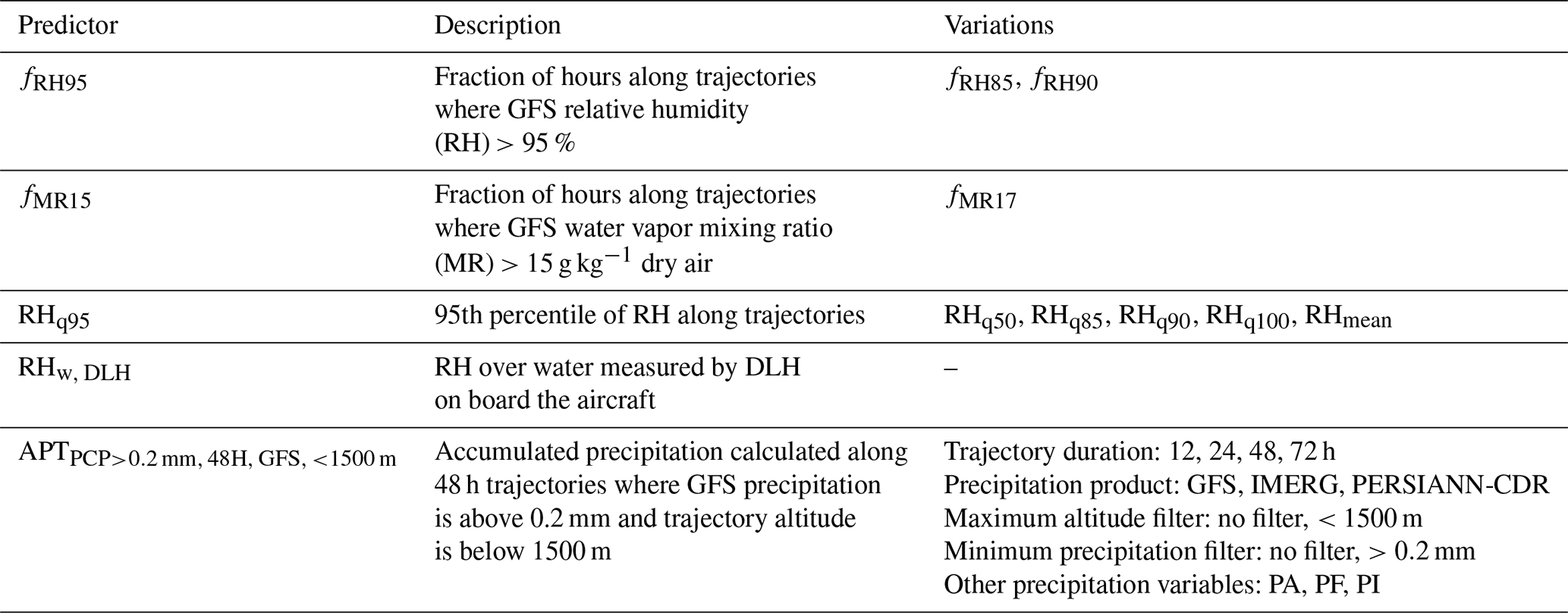
Besides APT, we also calculated precipitation amount (PA; mm h−1), frequency (PF), and intensity (PI; mm h−1), which are well-established in the literature for characterizing precipitation, particularly in diurnal cycle analyses (e.g., Zhang et al., 2017; Hilario et al., 2020). Applying these quantities to precipitation along trajectories, PA is APT divided by the total number of hours along the trajectory (i.e., trajectory length) to obtain an average hourly precipitation rate, PF is the fraction of hours along the trajectory where the grid cell precipitation is above 0 mm h−1, and PI is the ratio of PA to PF. Table 1 shows notation used to explain each type of predictor and its variations.
2.7 Curve fitting and k-fold cross-validation
To quantify relationships between TEBC and each predictor as well as its uncertainty, we performed k-fold cross-validation (k=10) parallelized using the Python package Jug version 2.2.2 (Coelho, 2017). To create k distinct partitions of the data, we utilized stratified random sampling wherein random sampling was performed for each 5th percentile block of the predictor such that the sampling probability better reflects the distribution of predictor values, which is important for skewed distributions such as precipitation amount, and the resulting k partitions capture the behavior of TEBC across the full spectrum of predictor values. By randomly sampling each percentile block for k distinct partitions, this sampling method improves the chances of capturing intra-block variability in TEBC by collecting the most samples where the highest data coverage exists. The random nature of the sampling also allows for the consideration of extreme values in the curve fitting, with a sampling probability proportional to the frequency of these extreme values. As an example, Fig. 1a–b show the emphasis of the stratified random sampling method on high-density areas of the scatterplot of RHq90 and TEBC, denoted by dense percentile blocks (dashed gray lines). For extremely skewed distributions such as APT, several of the lower-value percentiles exhibited non-unique values (e.g., zero). In the case of repeated percentile values, these percentile-based groups were merged. We imposed a minimum of six distinct percentile blocks to ensure robust curve fitting.
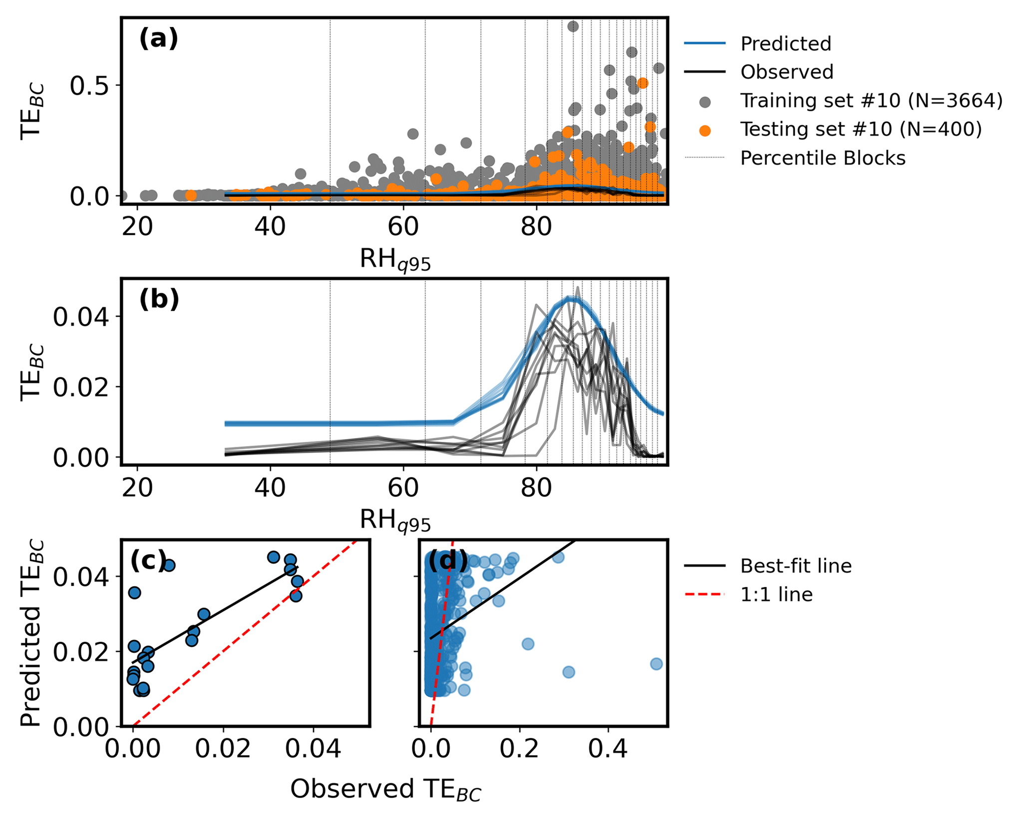
Figure 1An example of the curve-fitting procedure on TEBC with RHq95 as the predictor fitted with a Gaussian function. (a) Training (gray dots) and testing sets (orange dots) for the 10th iteration of the k-fold cross-validation procedure selected using stratified random sampling. Percentile blocks of each x-axis variable are denoted by vertical gray lines with observed (black) and predicted curves (blue) also plotted for all 10 iterations. (b) Same as panel (a) but only showing observed (black) and predicted curves (blue) for all 10 iterations to highlight variations between the k iterations. (c) Scatterplot comparing RHq95-predicted and observed median TEBC per 5th percentile block of the predictor. Note that panel (c) is simply the linear regression of the observed and predicted curves in panel (b). (d) Same as panel (c) but comparing RHq95-predicted and observed TEBC for individual points. In panels (c)–(d), only training set data are used, y axes are the same, the best-fit line is shown as a black line, and the 1:1 line is the dashed red line.
An iterative train–test split procedure using these partitions was then performed using k−1 partitions as the training set and the remaining partition as the testing set (Fig. 1a). For each iteration of the k-fold cross-validation, nonlinear least-squares curve fitting was applied to the training set (i.e., nine partitions for a total k of 10) to determine coefficients for the equation (e.g., general exponential; discussed below) fitted onto the scatterplot of TEBC and the predictor. We used these coefficients and the testing set (i.e., the remaining partition) as inputs for the curve-fitting equation and calculated a predicted curve of TEBC and the predictor. To assess this predicted curve, we applied stratified random sampling to the testing set and took the median TEBC per 5th percentile block to create observed curves of TEBC as a function of the predictor that could be compared to the predicted curve (Fig. 1b). Because decreases in TEBC are expected to be mainly from wet scavenging, the overall trend or median curve may be treated as a reasonable indicator of wet scavenging effects on TEBC related to changes in the predictor value.
Using a linear regression of predicted and observed median TEBC per 5th percentile block of the predictor (Fig. 1c), we calculated statistics (e.g., slope, R) to describe how well the predictor can predict TEBC. Specifically, the performance of a predictor refers to how well TEBC derived from the predictor matches observed TEBC. We also computed statistics comparing predicted and observed TEBC for individual points (Fig. 1d) rather than medians to assess how much variability in TEBC is captured by the predicted curves. The population in Fig. 1d visually follows the 1-to-1 line, indicating good performance of the model; however, the best-fit line on individual points was greatly affected by outlier points of high observed TEBC that led to poor agreement between the best-fit and 1-to-1 lines when the actual agreement was much better (visually). This suggests that the median-based statistics (Fig. 1c) are more robust to outliers and present a fairer evaluation of model predictions. Note that the individual-point statistics (Fig. 1d) resulted in correlations and slopes further from ideal values compared to the median-based statistics. This is expected as individual TEBC data points exhibit large variability due to the influence of factors other than wet scavenging; however, a comparison of our results when using individual-point or the median-based statistics shows that they agree quite well qualitatively, with the relative ranking of predictors largely unchanged between the two types of statistics. In other words, the top predictors performed well whether we used median-based or individual-point statistics, implying that the conclusions reached using our method are qualitatively insensitive to this choice. For simplicity, reported statistics in this study refer to median-based statistics unless otherwise specified.
To determine if a predictor tended to overestimate or underestimate TEBC, we calculated a weighted area difference (WAD) using Eq. (1):
where xi is the difference between observed and predicted TEBC for the ith percentile block and Ni is the number of data points in that percentile block. A positive (negative) WAD indicates an overestimate (underestimate) of observed TEBC.
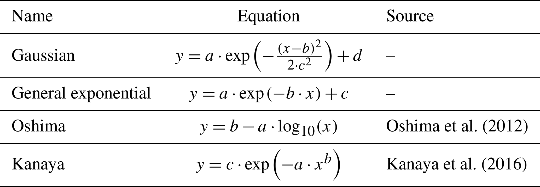
To account for differing relationships between TEBC and each predictor, we applied curve fitting to the scatterplot of each predictor and TEBC using multiple nonlinear equations (Table 2) and chose the equation that produced the highest Pearson correlation (R) between observed and predicted TEBC for that predictor. We considered equations from two previous studies (Kanaya et al., 2016; Oshima et al., 2012) and two generalized equations (Gaussian, general exponential) to capture other types of relationships (Table 2). The inclusion of the latter two are to account for a wider range of possible relationships between predictors and TEBC, such as the case of a predictor capturing TEBC trends well but not having an inversely proportional relationship with . The case of a non-inversely proportional relationship with TEBC is still interesting because a strong relationship implies that the variable could be used to estimate TEBC even if their relationship is nonmonotonic. The final assigned equations led to similar root mean squared error (RMSE) across predictors (Fig. S3), suggesting it is fair to compare different predictors.
Table 2Curve-fitting equations considered where x is the predictor variable and y is the observed , while a, b, c, and d are best-fit parameters determined via least-squares regression.
When selecting which equation to use (among those in Table 2) for fitting between the predictor and TEBC, we opted for the equation that resulted in the highest R between observed and predicted TEBC (e.g., Fig. 1c). The basis of this choice on R was because our objective is to identify predictors that can at least capture trends in TEBC. After selecting which equation to use per predictor, the subsequent comparison (Sect. 3) of the performance of different predictors considers other statistical metrics such as slope, intercept, and WAD. For some combinations of predictors and equations, the curve fitting did not successfully converge (<4 % of all combinations and k-fold iterations). In these cases, we did not include the predictor–equation combination in our analysis. However, curve fitting on the predictor may still converge when using a different equation. In such a scenario, the predictor becomes part of our analysis.
Sensitivity testing with the k value showed no significant effect on the general conclusions of the study when k was changed between 5 and 20 (not shown). We opted for k=10 based on previous work evaluating different accuracy estimation methods which showed that k=10 is sufficient to estimate performance metrics (e.g., R2) while minimizing computational expense (Breiman and Spector, 1992; Kohavi, 1995).
Although there is no physical process built into this procedure, the strength of the method is its repeatability in different environments or regions with minimal changes to the overall procedure. As it requires no physical model to be run besides the trajectory calculations, the method is also relatively computationally inexpensive. Future work wanting a more physical basis may apply our method as a diagnostic tool to identify and narrow down a list of meteorological variables that may be relevant to wet scavenging and continue their analysis with a physical model using the narrowed list of variables to analyze.
3.1 Overall statistical performance
Figures 2, 3, and S3 show performance comparisons of different predictors derived from linear regressions of observed and predicted TEBC. Hereafter, the performance of a predictor in this study refers to a predictor's ability to predict observed TEBC based on curve fitting (Sect. 2.7; Fig. 1c). To simplify these figures, only the top eight predictors per panel (by R) are colored to focus our discussion on predictors that were able to predict TEBC. Table S1 provides the equation and coefficients used for the top eight predictors per panel of Fig. 2.
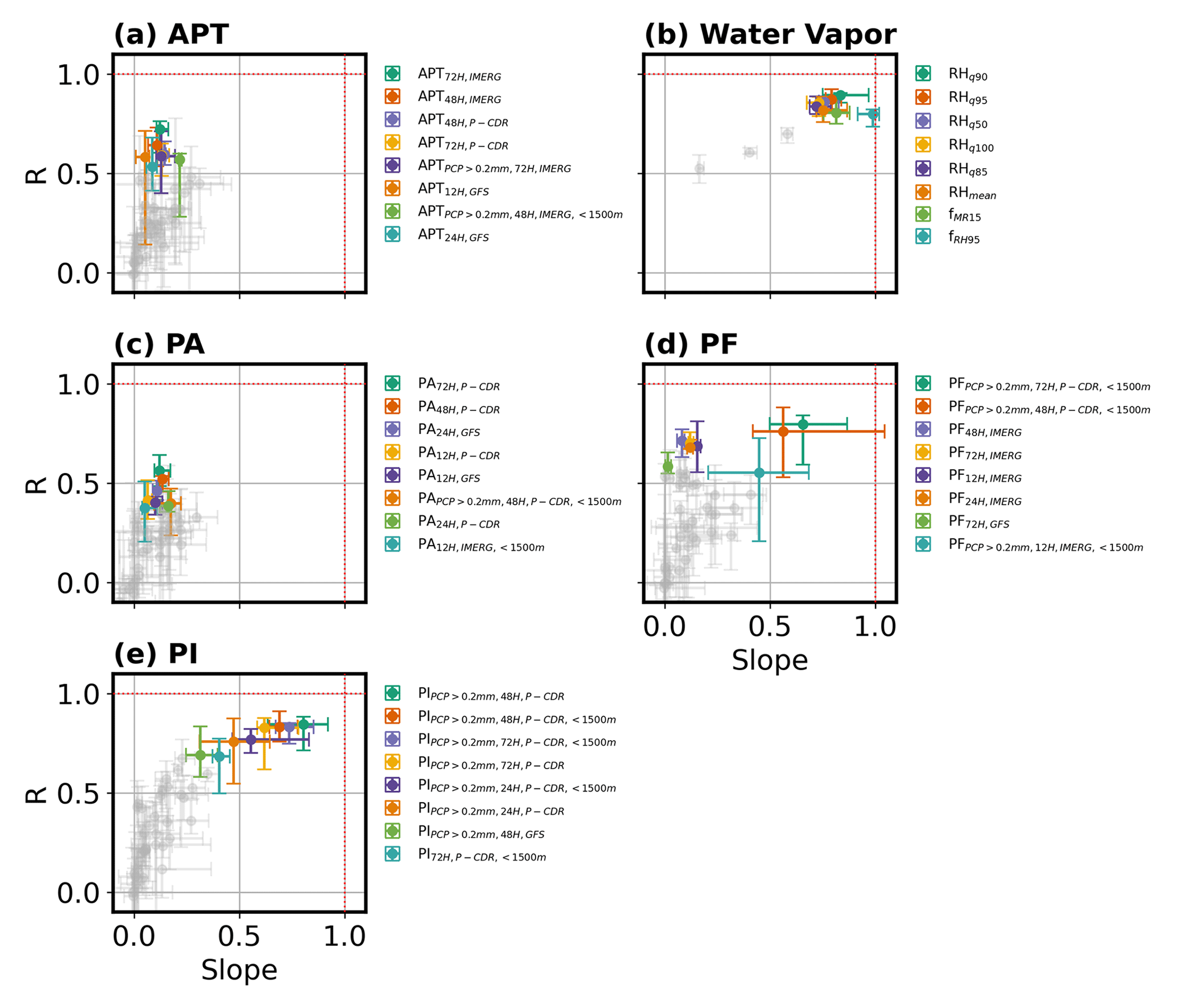
Figure 2Slope and Pearson correlation (R) values derived from linear regressions of observed (x) and predicted (y) TEBC with error bars representing the 25th and 75th percentile values derived from k-fold cross-validation (k=10) using stratified random sampling (Sect. 2.7). Ideal values are denoted by the dashed red lines such that a better predictor would fall closer to the intersection of the two lines. The top eight predictors per group (panel) are colored non-gray, while the rest of the predictors are plotted in gray to show the relative performance of all predictors. Note that PERSIANN-CDR has been abbreviated to P-CDR (b–c). Panels share the same x- and y-axis limits.
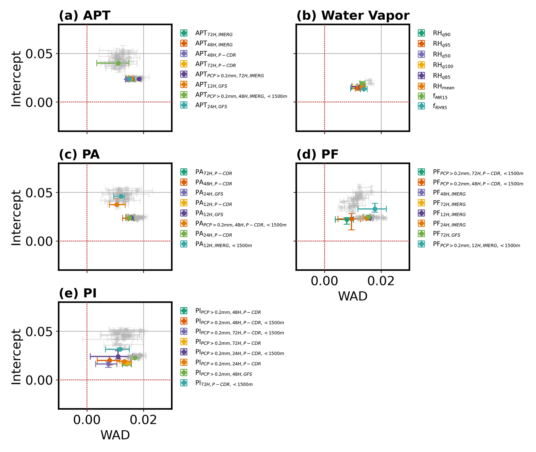
Figure 3Same as Fig. 2 but comparing intercept and weighted area difference (WAD, Sect. 2.7).
Using APT-based predictors (Fig. 2a) led to moderate R between predicted and observed TEBC but slopes far below the ideal value of 1, which, in addition to positive intercepts and WAD (Fig. S3a), indicate that APT-based predictors tend to underestimate TEBC when APT is high.
In comparison, predictors in Fig. 2b are based on RH (e.g., fRH95, RHq90) or MR (i.e., fMR15) and predicted TEBC much better in terms of trends (high R) and magnitude (slopes close to 1), suggesting that these predictors (Fig. 2b) could be better at estimating TEBC than APT (Fig. 2a). One possibility for this is that APT is an accumulated value that does not account for frequency or intensity, both of which have been argued to be important for regulating aerosol scavenging (Hou et al., 2018; Y. Wang et al., 2021b). To explore this possibility further, we calculated PA, PF, and PI for each trajectory (Fig. 2c–e). Among these three, PF (Fig. 2d) and PI (Fig. 2e) resulted in the best slopes and R, with PI showing slightly better slopes and R than PF. In comparison, PA performed poorly, similar to APT, which is expected as both are related to summed precipitation amount. Comparing the PI variables with the highest R (i.e., colored points in Fig. 2e), the majority of these good-performing PI variables were filtered for heavier or more intense precipitation (i.e., >0.2 mm). This filtering for heavier precipitation was done by including only grid cells with precipitation >0.2 mm when calculating PI. A similarly good performance was observed for PF variables that also filtered for more intense precipitation. These results suggest that PI (and to a lesser degree PF) must be accounted for when predicting aerosol scavenging over the tropical western Pacific. This further implies that even though precipitation may be occurring, it may not be efficiently scavenging aerosol.
Comparing which precipitation products are among the top predictors (by R), most good-performing precipitation-based predictors used SPP-based precipitation such as IMERG or PERSIANN-CDR (Fig. 2c–e). This suggests that GFS-derived precipitation variables are not as able to capture observed TEBC trends. The poor performance of GFS-derived precipitation is reflective of past studies showing disagreements in precipitation characteristics between satellites and reanalyses (Cannon et al., 2017; Jiang et al., 2021) and even divergent precipitation trends and amounts among individual reanalysis products (Alexander et al., 2020; S. Chen et al., 2020; Barrett et al., 2020). Our results corroborate previous work that precipitation from GFS reanalysis is not a reliable predictor of aerosol scavenging compared to precipitation from SPPs. Future studies relating precipitation to aerosol scavenging are recommended to instead rely on in situ or satellite-retrieved precipitation rather than precipitation from reanalysis.
Predictors based on quantiles of RH (e.g., RHq90) (Fig. 2b) perform quite well, with high R and slope (Fig. 2e) as well as intercept and WAD consistently close to 0 regardless of quantile (Fig. 3b). RHq90 performs slightly better in terms of R than other RH thresholds (Fig. 2b); however, this difference is minor as shown by the overlapping 25th–75th percentile error bars between the different RH quantiles. The similar performance between different RH quantiles suggests consistency in their ability to predict TEBC trends (high R; Fig. 2b) while doing reasonably better than other types of predictors when estimating TEBC magnitudes across the spectrum of predictor values (intercepts closer to 0, slopes closer to 1). Maximum RH along trajectories was used by Kanaya et al. (2016) in their analysis of scavenging to detect the role of clouds in BC removal. Our findings suggest that top quantiles of RH, including its maximum, are good choices for estimating TEBC.
Compared to variables directly linked to precipitation (PA, PF, PI, APT), the slopes from RH quantiles are noticeably closer to the ideal value of 1 (Fig. 2b), while their intercepts are closer to the ideal value of 0 (Fig. 2b), meaning TEBC predicted by RH quantiles more closely matches the observed TEBC than TEBC predicted by precipitation. We hypothesize that the better performance of RH-related predictors over those more directly related to precipitation (e.g., APT) may be explained by instances of precipitation that are missed (or misestimated) by SPP retrievals that are indirectly detected by reanalysis as high humidity conditions. This possibility is supported by previous literature showing the tendency of SPPs to misestimate light (Nadeem et al., 2022; Kidd et al., 2021) or intense precipitation (H. Chen et al., 2020; Gupta et al., 2020); however, we cannot rule out the possibility of the hygroscopic growth, in-cloud activation (high RH), and subsequent removal of BC during transport. Thus, our hypothesis of RH from reanalysis capturing missed precipitation from SPPs requires further investigation in future work.
Of all the fractional predictors considered in this study, fMR15 and fRH95 perform the best (Fig. 2b). fMR15 and fRH95 reflect the frequency of occurrence of scavenging-conducive conditions during transport. A high frequency of high MR or RH may indicate that air masses passed through large areas of clouds and/or precipitation during long-range transport. fRH95 has a median slope of 0.99 (Fig. 2b), a 25th–75th percentile range in slope of 0.92–1.02 (Fig. 2b), and a median intercept of 0.01 (Fig. 3b), indicating that fRH95 can be used to capture TEBC trends and magnitudes for a wide range of TEBC. The good performance of fMR15 and fRH95 suggests that the frequency of scavenging-conducive conditions may be a more reliable indicator of aerosol scavenging than precipitation amount (e.g., APT, PA).
3.2 Nonlinear sensitivity of TEBC to meteorological variables
Although the predictors in Figs. 2–3 exhibit the highest R of all predictors considered in this study, their slopes are generally below 1 (Fig. 2), while their intercepts and WAD are generally positive (Fig. 3). The combination of these statistics implies that predictions of TEBC using our method tend to overestimate observed TEBC across the spectrum of predictor values (indicated by WAD >0) with maximum overestimations occurring when observed TEBC is low (indicated by slopes <1 and intercepts >0). This points to a nonlinear sensitivity of TEBC to these predictors as the degree of scavenging increases. Dadashazar et al. (2021) observed a similar nonlinear response to APT by a ratio of particulate matter below 2.5 µm to CO (ΔPMCO), where ΔPMCO was most responsive to APT when APT was below 5 mm and less sensitive to APT when APT exceeded 5 mm.
Investigating this sensitivity further, Fig. 4 shows that PF-predicted TEBC does not capture the trends of observed TEBC for highly scavenged air masses. In other words, PF loses its predictive power as the degree of scavenging increases, implying that PF is most important for the scavenging of fresher air masses (high TEBC). This nonlinear sensitivity of TEBC to PF hints at the possibility that other meteorological variables may become important for further scavenging of highly scavenged air (low TEBC). In contrast to predictors directly related to precipitation (Fig. 4d–f), the predicted curves of RHq95 (Fig. 4a), fRH95 (Fig. 4b), and fMR15 (Fig. 4c) visibly track the trends of observed TEBC with approximately half the difference between predicted and observed TEBC when TEBC is low. The capability of RHq95, fRH95, and fMR15 to predict TEBC across a wider range of values is further reflected by generally lower intercepts and WAD (Fig. 3) than precipitation-related predictors, which suggests promising alternative indicators of aerosol scavenging. However, we also note that such differences could arise partly from the limitations of curve fitting, wherein fitted curves naturally capture gradual changes (e.g., Fig. 4b) better than sharp ones (e.g., Fig. 4d).
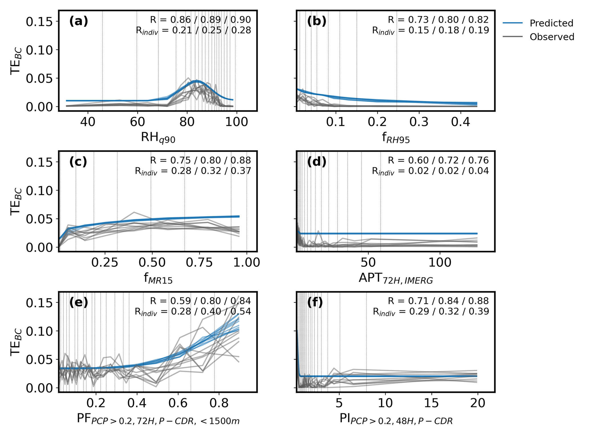
Figure 4Median values of observed (black) and predicted TEBC (blue) as a function of selected predictors for 10 iterations during k-fold cross-validation. Pearson correlations are annotated as 25th, 50th, and 75th percentiles from k-fold iterations (k=10) calculated in two ways: comparing predicted and observed median TEBC per 5th percentile block of the predictor (R) and comparing predicted and observed TEBC for individual points (Rindiv). Panels share the same y-axis limits. Percentile blocks for each x-axis variable are denoted by vertical gray lines.
3.3 Applying filters to improve the predictive power of precipitation-related variables
In this section, we examine the predictive power of precipitation-related variables when applying the following filters: (1) precipitation intensity, (2) trajectory altitude, (3) data product, and (4) trajectory length, with the objective of identifying what factors are important when relating precipitation along trajectories to TEBC. Filtering for precipitation intensity isolates the contribution of higher precipitation intensities towards a precipitation-related predictor's ability to predict TEBC. Intense precipitation has been shown to be more efficient at scavenging aerosol particles (Zhao et al., 2020) and may be important when estimating aerosol scavenging. Filtering for trajectory altitude (i.e., considering precipitation only when the trajectory altitude is below 1.5 km a.g.l.) tests the hypothesis that air masses within the boundary layer will be most susceptible to wet scavenging. Grythe et al. (2017) demonstrated that below-cloud scavenging (i.e., impaction by precipitation) accounted for the majority of scavenging events below 1 km. We selected 1.5 km based on previous work on the marine boundary layer over the tropical western Pacific (Chien et al., 2019). We repeated the analysis for three precipitation products (one reanalysis and two SPPs) to capture variability in our results due to the choice of data product, which has been shown to be important for precipitation (Alexander et al., 2020). Finally, we tested the effect of trajectory length on the performance of APT as a predictor of TEBC. We performed these sensitivity tests on APT (Fig. 5), PI (Fig. S4), PF (Fig. S5), and PA (Fig. S6).
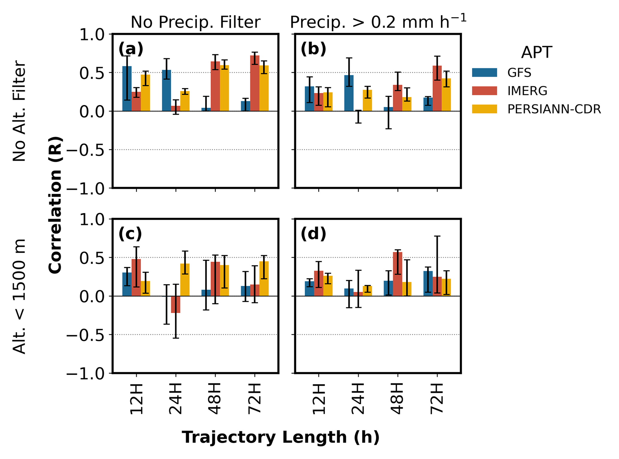
Figure 5Pearson correlations (R) between observed TEBC and TEBC predicted by accumulated precipitation along trajectories (APT) for different trajectory lengths and precipitation data products. Each panel refers to a combination of altitude and precipitation intensity filters. Panels share the same x- and y-axis limits.
In general, we found that applying altitude and/or precipitation filters negatively affected the performance of APT (Fig. 5b–d), PF (Fig. S5b–d, except for PERSIANN-CDR), and PA (Fig. S6b–d), leading to lower R between predicted and observed TEBC compared to the case without any filters (Fig. 5a). Two exceptions were PF from PERSIANN-CDR (colored yellow in Fig. S5), which could be used to estimate TEBC if we applied both an altitude filter (<1500 m) and a precipitation intensity filter (>0.2 mm h−1) over longer back-trajectory times (>48 h) (Fig. S5d), and PI, which could be used to estimate TEBC when filtering for precipitation intensities (>0.2 mm h−1) and along trajectories longer than 48 h (Fig. S4b). The better performance of PI across multiple SPPs (Fig. S4) is an encouraging sign that this improvement is robust and points to the contribution of higher precipitation intensities towards total scavenging.
Applying a filter for trajectory altitude prior to calculating APT also did not lead to large improvements in R (Fig. 5c). This was surprising because, when using total column precipitation from SPPs, a maximum altitude filter should reduce errors from cases in which precipitation occurs below the air mass and no scavenging occurs. Since the SPPs used in this study have been validated using surface measurements (Sapiano and Arkin, 2009; Nicholson et al., 2019; J. Wang et al., 2021), precipitation from SPPs should be reflective of precipitation that reaches the surface, implying a susceptibility of these SPPs to errors related to virga (Wang et al., 2018). However, Wang et al. (2018) also showed that virga occurrence over the tropical western Pacific is infrequent. An alternative explanation for the poor performance of altitude-filtered APT is uncertainties related to trajectory altitude (Harris et al., 2005) such that an air parcel may have actually been traveling at a lower altitude than its modeled trajectory and undergone more scavenging than predicted using APT. An examination of trajectory altitudes (Fig. S7) revealed that filtering for trajectory altitudes below 1.5 km excluded the majority (∼ 70 %) of precipitating grid cells encountered by trajectories, which likely negatively impacted the predictive ability of altitude-filtered predictors.
Longer trajectories resulted in slightly higher R between observed and predicted TEBC using APT from PERSIANN-CDR or IMERG (Fig. 5a–b); however, this difference is not large, as shown by overlapping 25th–75th percentile error bars. Interestingly, this increase in R for longer trajectories was more evident when filtering for precipitation intensities >0.2 mm h−1 when calculating APT (Fig. 5b) or PI (Fig. S4b), but not when applying this intensity filter to PF (Fig. S3b) or PA (Fig. S4b). Further interpretation likely requires a physical model in future work to explain why the performance of intense precipitation (Fig. 5b) benefits from a longer trajectory more than total precipitation does (Fig. 5a).
4.1 TEBC as a wet scavenging proxy
In this study, we treat TEBC as a proxy for wet scavenging (i.e., predictand) and base our conclusions on which variables (i.e., predictors) best predict TEBC. Dilution or entrainment during transport is expected to influence the ratio and therefore TEBC. While the use of the CAMS-GLOB-ANT emission inventory (Sect. 2.4) when calculating ER (Sect. 2.5) reduces this uncertainty by accounting for potential surface influence during transport close to the surface, the resolutions of both the trajectory meteorological input (0.25 × 0.25∘) and the emission inventory (0.1 × 0.1∘) remain limiting factors. Thus, our analysis assumes that wet scavenging is the main driver of changes in TEBC and chemical transport modeling in future work is needed to quantify the effect of mixing on TEBC. Consequently, this method is expected to work well in outflow regions such as the tropical western Pacific and not well where additional BC and/or CO are likely to be after initial emission or wet scavenging has occurred (e.g., continental region).
4.2 Method does not discriminate between in- and below-cloud scavenging
The conclusions of our study are based on the relative ability of different variables to predict TEBC, our proxy for wet scavenging. This approach does not isolate individual processes that are usually parameterized by global circulation models (e.g., impaction, nucleation) (Croft et al., 2009, 2010; Ryu and Min, 2022) and does not discriminate between in-cloud or below-cloud scavenging. However, through our proposed framework, we can still gain qualitative insights into which meteorological variables are relevant for estimating aerosol scavenging, which can inform future studies as well as developments in model parameterization.
4.3 Single-predictor method
The method presented here assesses the one-to-one relationship between a single predictor and TEBC repeated individually for several predictors. We expect that using a combination of predictors may lead to better predictions of TEBC while providing a more physical picture of relative contributions of different meteorological variables to wet scavenging. Future work may utilize multiple linear regression or more sophisticated methods such as machine learning to consider different combinations of predictors with the objective of identifying a combination that predicts TEBC well and extracting further information on what physical mechanisms may be relevant for the removal of TEBC based on relative coefficients or weightings of different predictors.
4.4 Curve fitting
The results can depend on the curve-fitting function used. Different variables are expected to have different relationships with TEBC. Thus, considering only one function for curve fitting favors variables that have a specific relationship with TEBC. To reduce this bias, we applied four different curve-fitting functions (Table 2) to each predictor based on two equations from previous studies (Kanaya et al., 2016; Oshima et al., 2012) and two equations of generalized form that accounted for possible relationships between TEBC and each predictor. We then chose the curve-fitting function that produced the highest R between observed and predicted TEBC. However, we note that this does not completely remove the bias as specific functions were still selected.
4.5 Trajectory modeling
Vertical motion through convection, entrainment, and detrainment processes is a known uncertainty in trajectory modeling, which increases with trajectory length (Harris et al., 2005). The spatial and temporal resolutions of the meteorological input used for the HYSPLIT model are also limiting factors as meteorology along HYSPLIT trajectories do not account for sub-time-step or sub-grid processes.
We present a method to identify meteorological indicators of aerosol scavenging using a combination of aircraft, satellite, and reanalysis data coupled with HYSPLIT backward trajectories. We apply this method to the CAMP2Ex field campaign over the tropical western Pacific, which hosts a wide range of cloud fractions and precipitation characteristics as well as an environment characterized by long-range transport of aerosol and trace gas species. We evaluate which meteorological variables can be used to predict TEBC (i.e., predictors). The main conclusions of the study are the following.
- 1.
Although APT has been utilized in several studies as an indicator of aerosol scavenging, we demonstrate that APT does poorly when predicting TEBC (e.g., weak correlations, underestimates TEBC). Furthermore, the application of altitude or precipitation intensity filters negatively impacts the performance of APT in predicting TEBC. Since APT is an accumulated precipitation amount over the whole trajectory, APT does not account for other precipitation characteristics such as intensity or frequency, which have been shown to be relevant for aerosol scavenging. This shortcoming may explain the overall poor relative performance of APT in predicting TEBC.
- 2.
Predictors based on specific quantiles of RH (e.g., RHq90) also perform quite well in predicting both TEBC trends and magnitudes (intercepts close to zero, WAD close to zero, slopes close to 1, R close to 1). We find only minor differences in the performance depending on the exact quantile used, suggesting that the RH distribution during transport is a robust way to estimate TEBC. We hypothesize the outperformance of RH quantiles over predictors more directly related to precipitation (e.g., APT) to be due to missed precipitation in SPP retrievals that was indirectly represented in reanalysis as high humidity conditions; however, further work is required to explore this possibility.
- 3.
Frequency-related predictors such as fMR15 and fRH95 perform better than APT in predicting TEBC trends (higher R) and magnitudes (slopes closer to 1). fMR15 and fRH95 represent the frequencies along 72 h trajectories of MR exceeding 15 g kg−1 and RH exceeding 95 %, respectively. The abilities of fMR15 and fRH95 to predict TEBC suggests that the frequency of humid conditions should be considered when estimating aerosol scavenging.
- 4.
To investigate which precipitation characteristics are most relevant for predicting TEBC, we quantify PA, PF, and PI along trajectories and find that PI is the most effective at estimating TEBC when we calculate PI over longer trajectories (>48 h) and only include grid cells with precipitation >0.2 mm h−1 in our calculation. This points to the contribution of intense precipitation and the importance of accounting for air mass history when estimating aerosol scavenging.
- 5.
We find that precipitation from SPPs (IMERG, PERSIANN-CDR) is generally better at predicting TEBC (higher R) than precipitation from reanalysis (GFS). This is corroborated by previous studies that found larger misestimates of precipitation by reanalysis than by SPPs. Because of our results and those of past studies, we recommend relying on in situ or SPP precipitation rather than precipitation from reanalysis, particularly when relating precipitation to aerosol scavenging.
Given these findings, we recommend the following alternatives to APT when estimating aerosol scavenging: (1) RH quantiles (e.g., 90th percentile of RH along trajectories), (2) fMR15 or fRH95, and (3) PI from SPPs filtered for grid cells with precipitation >0.2 mm h−1. These variables were found to be able to predict TEBC more accurately than APT; thus, future scavenging parameterizations should consider these meteorological variables along air mass histories.
Future work is encouraged to apply this method over a variety of environments (e.g., using other data from other field campaigns), utilize machine learning to assess what combinations of meteorological variables are relevant for predicting aerosol scavenging, and apply this method to other regions to determine if there are regional differences in indicators of aerosol scavenging. Furthermore, CAMP2Ex included a rich dataset on cloud water composition (Crosbie et al., 2022; Stahl et al., 2021) that can be explored, as in past work for other regions (MacDonald et al., 2018), to gain additional insights into aerosol wet scavenging processes.
During the CAMP2Ex field campaign, BC and CO originated from several sources. Long-range transport patterns during the campaign and associated air mass composition are described in Hilario et al. (2021), but here we present a summary of their findings related to the transport of BC and CO. The CAMP2Ex field campaign overlapped with the end of the southwest monsoon and the beginning of the monsoon transition (Reid et al., 2023). Because of this, a synoptic shift occurred during the campaign (Hilario et al., 2021; their Figs. 2–3) that allowed for the sampling of transported air masses from different source regions such as East Asia and the Maritime Continent. Hilario et al. (2021) identified four major source regions for long-range transport: East Asia (e.g., China, Korea), the Maritime Continent (e.g., Indonesia, Malaysia), peninsular Southeast Asia (e.g., Vietnam), and the western Pacific (i.e., ocean). The presence of long-range transport was detected throughout the whole campaign (their Fig. S2).
The Maritime Continent during the campaign was undergoing its burning season, which is well-established in the literature to lead to high aerosol loadings that can be transported over large distances (Xian et al., 2013). Hilario et al. (2021) showed that air masses from the Maritime Continent and East Asia were transported under relatively dry conditions, which in this study manifested as higher (Fig. S1a) and TEBC (Fig. S1d), and were associated with southwesterly monsoon flow and the passage of typhoons, respectively. These conditions were conducive to long-range transport and led to the sampling of higher concentrations of BC and CO in air from East Asia (BC: 87.29 ng m−3; CO: 0.16 ppm) and the Maritime Continent (BC: 71.81 ng m−3; CO: 0.18 ppm) than in air from peninsular Southeast Asia (BC: 24.90 ng m−3; CO: 0.10 ppm) or the western Pacific (BC: 1.03 ng m−3; CO: 0.08 ppm). We note that Hilario et al. (2021a) kept CO in units of parts per million, while we converted CO to mass concentration units such that would be unitless. Hilario et al. (2021a) demonstrated that the scavenging of air from peninsular Southeast Asia was related to convective lofting as air from peninsular Southeast Asia sampled in the free troposphere (>1.5 km) had much lower aerosol concentrations than air from the region sampled in the boundary layer (<1.5 km) (their Fig. S6). These findings point to the active role of scavenging in determining aerosol loadings in transported air masses during CAMP2Ex.
Codes are freely available upon request to the authors.
All datasets are publicly available and accessible at https://doi.org/10.5067/Suborbital/CAMP2EX2018/DATA001 (CAMP2Ex Science Team, 2019). HYSPLIT data are accessible through the NOAA READY website (https://www.ready.noaa.gov/index.php, last access: 13 June 2020, NOAA Physical Sciences Laboratory).
The supplement related to this article is available online at: https://doi.org/10.5194/amt-17-37-2024-supplement.
ECC, LDZ, MAS, JPD, and GSD contributed to data collection. MRAH and AS conceptualized the study. MRAH performed the data analysis and prepared the paper with input from all co-authors.
The contact author has declared that none of the authors has any competing interests.
Publisher's note: Copernicus Publications remains neutral with regard to jurisdictional claims made in the text, published maps, institutional affiliations, or any other geographical representation in this paper. While Copernicus Publications makes every effort to include appropriate place names, the final responsibility lies with the authors.
This article is part of the special issue “Cloud Aerosol and Monsoon Processes Philippines Experiment (CAMP2Ex) (ACP/AMT inter-journal SI)”. It is not associated with a conference.
The authors gratefully acknowledge the financial support of the National Aeronautics and Space Administration.
This research has been supported by the National Aeronautics and Space Administration (grant no. 80NSSC18K0148).
This paper was edited by Edward Nowottnick and reviewed by two anonymous referees.
Alexander, L. V., Bador, M., Roca, R., Contractor, S., Donat, M. G., and Nguyen, P. L.: Intercomparison of annual precipitation indices and extremes over global land areas from in situ, space-based and reanalysis products, Environ. Res. Lett., 15, 055002, https://doi.org/10.1088/1748-9326/ab79e2, 2020.
Andronache, C.: Estimated variability of below-cloud aerosol removal by rainfall for observed aerosol size distributions, Atmos. Chem. Phys., 3, 131–143, https://doi.org/10.5194/acp-3-131-2003, 2003.
Ashouri, H., Hsu, K.-L., Sorooshian, S., Braithwaite, D. K., Knapp, K. R., Cecil, L. D., Nelson, B. R., and Prat, O. P.: PERSIANN-CDR: Daily Precipitation Climate Data Record from Multisatellite Observations for Hydrological and Climate Studies, B. Am. Meteorol. Soc., 96, 69–83, https://doi.org/10.1175/BAMS-D-13-00068.1, 2015.
Barrett, A. P., Stroeve, J. C., and Serreze, M. C.: Arctic Ocean Precipitation From Atmospheric Reanalyses and Comparisons With North Pole Drifting Station Records, J. Geophys. Res.-Oceans, 125, e2019JC015415, https://doi.org/10.1029/2019JC015415, 2020.
Bellouin, N., Quaas, J., Gryspeerdt, E., Kinne, S., Stier, P., Watson-Parris, D., Boucher, O., Carslaw, K. S., Christensen, M., Daniau, A.-L., Dufresne, J.-L., Feingold, G., Fiedler, S., Forster, P., Gettelman, A., Haywood, J. M., Lohmann, U., Malavelle, F., Mauritsen, T., McCoy, D. T., Myhre, G., Mülmenstädt, J., Neubauer, D., Possner, A., Rugenstein, M., Sato, Y., Schulz, M., Schwartz, S. E., Sourdeval, O., Storelvmo, T., Toll, V., Winker, D., and Stevens, B.: Bounding Global Aerosol Radiative Forcing of Climate Change, Rev. Geophys., 58, e2019RG000660, https://doi.org/10.1029/2019RG000660, 2020.
Breiman, L. and Spector, P.: Submodel Selection and Evaluation in Regression. The X-Random Case, Int. Stat. Rev., 60, 291–319, https://doi.org/10.2307/1403680, 1992.
CAMP2Ex Science Team: Clouds, Aerosol and Monsoon Processes-Philippines Experiment, NASA Langley Atmospheric Science Data Center DAAC [data set], https://doi.org/10.5067/SUBORBITAL/CAMP2EX2018/DATA001, 2019.
Cannon, F., Ralph, F. M., Wilson, A. M., and Lettenmaier, D. P.: GPM Satellite Radar Measurements of Precipitation and Freezing Level in Atmospheric Rivers: Comparison With Ground-Based Radars and Reanalyses, J. Geophys. Res.-Atmos., 122, 12747–12764, https://doi.org/10.1002/2017JD027355, 2017.
Chen, H., Yong, B., Qi, W., Wu, H., Ren, L., and Hong, Y.: Investigating the Evaluation Uncertainty for Satellite Precipitation Estimates Based on Two Different Ground Precipitation Observation Products, J. Hydrometeorol., 21, 2595–2606, https://doi.org/10.1175/JHM-D-20-0103.1, 2020.
Chen, S., Liu, B., Tan, X., and Wu, Y.: Inter-comparison of spatiotemporal features of precipitation extremes within six daily precipitation products, Clim. Dynam., 54, 1057–1076, https://doi.org/10.1007/s00382-019-05045-z, 2020.
Chien, F.-C., Hong, J.-S., and Kuo, Y.-H.: The Marine Boundary Layer Height over the Western North Pacific Based on GPS Radio Occultation, Island Soundings, and Numerical Models, Sensors, 19, 155, https://doi.org/10.3390/s19010155, 2019.
Choi, Y., Kanaya, Y., Takigawa, M., Zhu, C., Park, S.-M., Matsuki, A., Sadanaga, Y., Kim, S.-W., Pan, X., and Pisso, I.: Investigation of the wet removal rate of black carbon in East Asia: validation of a below- and in-cloud wet removal scheme in FLEXible PARTicle (FLEXPART) model v10.4, Atmos. Chem. Phys., 20, 13655–13670, https://doi.org/10.5194/acp-20-13655-2020, 2020.
Coelho, L. P.: Jug: Software for Parallel Reproducible Computation in Python, 5, 30, https://doi.org/10.5334/jors.161, 2017.
Crippa, M., Guizzardi, D., Muntean, M., Schaaf, E., Dentener, F., van Aardenne, J. A., Monni, S., Doering, U., Olivier, J. G. J., Pagliari, V., and Janssens-Maenhout, G.: Gridded emissions of air pollutants for the period 1970–2012 within EDGAR v4.3.2, Earth Syst. Sci. Data, 10, 1987–2013, https://doi.org/10.5194/essd-10-1987-2018, 2018.
Croft, B., Lohmann, U., Martin, R. V., Stier, P., Wurzler, S., Feichter, J., Posselt, R., and Ferrachat, S.: Aerosol size-dependent below-cloud scavenging by rain and snow in the ECHAM5-HAM, Atmos. Chem. Phys., 9, 4653–4675, https://doi.org/10.5194/acp-9-4653-2009, 2009.
Croft, B., Lohmann, U., Martin, R. V., Stier, P., Wurzler, S., Feichter, J., Hoose, C., Heikkilä, U., van Donkelaar, A., and Ferrachat, S.: Influences of in-cloud aerosol scavenging parameterizations on aerosol concentrations and wet deposition in ECHAM5-HAM, Atmos. Chem. Phys., 10, 1511–1543, https://doi.org/10.5194/acp-10-1511-2010 2010.
Crosbie, E., Ziemba, L. D., Shook, M. A., Robinson, C. E., Winstead, E. L., Thornhill, K. L., Braun, R. A., MacDonald, A. B., Stahl, C., Sorooshian, A., van den Heever, S. C., DiGangi, J. P., Diskin, G. S., Woods, S., Bañaga, P., Brown, M. D., Gallo, F., Hilario, M. R. A., Jordan, C. E., Leung, G. R., Moore, R. H., Sanchez, K. J., Shingler, T. J., and Wiggins, E. B.: Measurement report: Closure analysis of aerosol–cloud composition in tropical maritime warm convection, Atmos. Chem. Phys., 22, 13269–13302, https://doi.org/10.5194/acp-22-13269-2022, 2022.
Dadashazar, H., Alipanah, M., Hilario, M. R. A., Crosbie, E., Kirschler, S., Liu, H., Moore, R. H., Peters, A. J., Scarino, A. J., Shook, M., Thornhill, K. L., Voigt, C., Wang, H., Winstead, E., Zhang, B., Ziemba, L., and Sorooshian, A.: Aerosol responses to precipitation along North American air trajectories arriving at Bermuda, Atmos. Chem. Phys., 21, 16121–16141, https://doi.org/10.5194/acp-21-16121-2021, 2021.
Feng, J.: A 3-mode parameterization of below-cloud scavenging of aerosols for use in atmospheric dispersion models, Atmos. Environ., 41, 6808–6822, https://doi.org/10.1016/j.atmosenv.2007.04.046, 2007.
Flossmann, A. I., Hall, W. D., and Pruppacher, H. R.: A Theoretical Study of the Wet Removal of Atmospheric Pollutants. Part I: The Redistribution of Aerosol Particles Captured through Nucleation and Impaction Scavenging by Growing Cloud Drops, J. Atmos. Sci., 42, 583–606, https://doi.org/10.1175/1520-0469(1985)042<0583:ATSOTW>2.0.CO;2, 1985.
Frey, L., Bender, F. A.-M., and Svensson, G.: Processes controlling the vertical aerosol distribution in marine stratocumulus regions – a sensitivity study using the climate model NorESM1-M, Atmos. Chem. Phys., 21, 577–595, https://doi.org/10.5194/acp-21-577-2021, 2021.
Ge, C., Wang, J., and Reid, J. S.: Mesoscale modeling of smoke transport over the Southeast Asian Maritime Continent: coupling of smoke direct radiative effect below and above the low-level clouds, Atmos. Chem. Phys., 14, 159–174, https://doi.org/10.5194/acp-14-159-2014, 2014.
Granier, C., Darras, S., Denier van der Gon, H., Doubalova, J., Elguindi, N., Galle, B., Gauss, M., Guevara, M., Jalkanen, J.-P., Kuenen, J., Liousse, C., Quack, B., Simpson, D., and Sindelarova, K.: The Copernicus Atmosphere Monitoring Service global and regional emissions (April 2019 version), Copernicus Atmosphere Monitoring Service (CAMS) report, https://doi.org/10.24380/D0BN-KX16, 2019.
Grythe, H., Kristiansen, N. I., Groot Zwaaftink, C. D., Eckhardt, S., Ström, J., Tunved, P., Krejci, R., and Stohl, A.: A new aerosol wet removal scheme for the Lagrangian particle model FLEXPART v10, Geosci. Model Dev., 10, 1447–1466, https://doi.org/10.5194/gmd-10-1447-2017, 2017.
Gupta, V., Jain, M. K., Singh, P. K., and Singh, V.: An assessment of global satellite-based precipitation datasets in capturing precipitation extremes: A comparison with observed precipitation dataset in India, Int. J. Climatol., 40, 3667–3688, https://doi.org/10.1002/joc.6419, 2020.
Harris, J. M., Draxler, R. R., and Oltmans, S. J.: Trajectory model sensitivity to differences in input data and vertical transport method, J. Geophys. Res.-Atmos., 110, D14109, https://doi.org/10.1029/2004JD005750, 2005.
Hilario, M. R. A., Olaguera, L. M., Narisma, G. T., and Matsumoto, J.: Diurnal Characteristics of Summer Precipitation Over Luzon Island, Philippines, Asia-Pac. J. Atmos. Sci., 57, 573–585, https://doi.org/10.1007/s13143-020-00214-1, 2020.
Hilario, M. R. A., Crosbie, E., Shook, M., Reid, J. S., Cambaliza, M. O. L., Simpas, J. B. B., Ziemba, L., DiGangi, J. P., Diskin, G. S., Nguyen, P., Turk, F. J., Winstead, E., Robinson, C. E., Wang, J., Zhang, J., Wang, Y., Yoon, S., Flynn, J., Alvarez, S. L., Behrangi, A., and Sorooshian, A.: Measurement report: Long-range transport patterns into the tropical northwest Pacific during the CAMP2Ex aircraft campaign: chemical composition, size distributions, and the impact of convection, Atmos. Chem. Phys., 21, 3777–3802, https://doi.org/10.5194/acp-21-3777-2021, 2021.
Hilario, M. R. A., Bañaga, P. A., Betito, G., Braun, R. A., Cambaliza, M. O., Cruz, M. T., Lorenzo, G. R., MacDonald, A. B., Pabroa, P. C., Simpas, J. B., Stahl, C., Yee, J. R., and Sorooshian, A.: Stubborn aerosol: why particulate mass concentrations do not drop during the wet season in Metro Manila, Philippines, Environ. Sci.: Atmos., 2, 1428–1437, https://doi.org/10.1039/D2EA00073C, 2022.
Hodzic, A., Kasibhatla, P. S., Jo, D. S., Cappa, C. D., Jimenez, J. L., Madronich, S., and Park, R. J.: Rethinking the global secondary organic aerosol (SOA) budget: stronger production, faster removal, shorter lifetime, Atmos. Chem. Phys., 16, 7917–7941, https://doi.org/10.5194/acp-16-7917-2016, 2016.
Hoesly, R. M., Smith, S. J., Feng, L., Klimont, Z., Janssens-Maenhout, G., Pitkanen, T., Seibert, J. J., Vu, L., Andres, R. J., Bolt, R. M., Bond, T. C., Dawidowski, L., Kholod, N., Kurokawa, J.-I., Li, M., Liu, L., Lu, Z., Moura, M. C. P., O'Rourke, P. R., and Zhang, Q.: Historical (1750–2014) anthropogenic emissions of reactive gases and aerosols from the Community Emissions Data System (CEDS), Geosci. Model Dev., 11, 369–408, https://doi.org/10.5194/gmd-11-369-2018, 2018.
Hou, P., Wu, S., McCarty, J. L., and Gao, Y.: Sensitivity of atmospheric aerosol scavenging to precipitation intensity and frequency in the context of global climate change, Atmos. Chem. Phys., 18, 8173–8182, https://doi.org/10.5194/acp-18-8173-2018, 2018.
Huffman, G. J., Bolvin, D. T., Braithwaite, D., Hsu, K.-L., Joyce, R. J., Kidd, C., Nelkin, E. J., Sorooshian, S., Stocker, E. F., Tan, J., Wolff, D. B., and Xie, P.: Integrated Multi-satellite Retrievals for the Global Precipitation Measurement (GPM) Mission (IMERG), in: Satellite Precipitation Measurement: Volume 1, edited by: Levizzani, V., Kidd, C., Kirschbaum, D. B., Kummerow, C. D., Nakamura, K., and Turk, F. J., Springer International Publishing, Cham, 343–353, https://doi.org/10.1007/978-3-030-24568-9_19, 2020.
Jalkanen, J.-P., Johansson, L., Kukkonen, J., Brink, A., Kalli, J., and Stipa, T.: Extension of an assessment model of ship traffic exhaust emissions for particulate matter and carbon monoxide, Atmos. Chem. Phys., 12, 2641–2659, https://doi.org/10.5194/acp-12-2641-2012, 2012.
Jensen, J. B. and Charlson, R. J.: On the efficiency of nucleation scavenging, Tellus B, 36, 367–375, https://doi.org/10.1111/j.1600-0889.1984.tb00255.x, 1984.
Jiang, Q., Li, W., Fan, Z., He, X., Sun, W., Chen, S., Wen, J., Gao, J., and Wang, J.: Evaluation of the ERA5 reanalysis precipitation dataset over Chinese Mainland, J. Hydrol., 595, 125660, https://doi.org/10.1016/j.jhydrol.2020.125660, 2021.
Kanaya, Y., Pan, X., Miyakawa, T., Komazaki, Y., Taketani, F., Uno, I., and Kondo, Y.: Long-term observations of black carbon mass concentrations at Fukue Island, western Japan, during 2009–2015: constraining wet removal rates and emission strengths from East Asia, Atmos. Chem. Phys., 16, 10689–10705, https://doi.org/10.5194/acp-16-10689-2016, 2016.
Kanaya, Y., Yamaji, K., Miyakawa, T., Taketani, F., Zhu, C., Choi, Y., Komazaki, Y., Ikeda, K., Kondo, Y., and Klimont, Z.: Rapid reduction in black carbon emissions from China: evidence from 2009–2019 observations on Fukue Island, Japan, Atmos. Chem. Phys., 20, 6339–6356, https://doi.org/10.5194/acp-20-6339-2020, 2020.
Kidd, C., Graham, E., Smyth, T., and Gill, M.: Assessing the Impact of Light/Shallow Precipitation Retrievals from Satellite-Based Observations Using Surface Radar and Micro Rain Radar Observations, Remote Sens.-Basel, 13, 1708, https://doi.org/10.3390/rs13091708, 2021.
Kim, K. D., Lee, S., Kim, J.-J., Lee, S.-H., Lee, D., Lee, J.-B., Choi, J.-Y., and Kim, M. J.: Effect of Wet Deposition on Secondary Inorganic Aerosols Using an Urban-Scale Air Quality Model, Atmosphere, 12, 168, https://doi.org/10.3390/atmos12020168, 2021.
Kipling, Z., Stier, P., Johnson, C. E., Mann, G. W., Bellouin, N., Bauer, S. E., Bergman, T., Chin, M., Diehl, T., Ghan, S. J., Iversen, T., Kirkevåg, A., Kokkola, H., Liu, X., Luo, G., van Noije, T., Pringle, K. J., von Salzen, K., Schulz, M., Seland, Ø., Skeie, R. B., Takemura, T., Tsigaridis, K., and Zhang, K.: What controls the vertical distribution of aerosol? Relationships between process sensitivity in HadGEM3–UKCA and inter-model variation from AeroCom Phase II, Atmos. Chem. Phys., 16, 2221–2241, https://doi.org/10.5194/acp-16-2221-2016, 2016.
Kleinman, L. I., Daum, P. H., Lee, Y.-N., Senum, G. I., Springston, S. R., Wang, J., Berkowitz, C., Hubbe, J., Zaveri, R. A., Brechtel, F. J., Jayne, J., Onasch, T. B., and Worsnop, D.: Aircraft observations of aerosol composition and ageing in New England and Mid-Atlantic States during the summer 2002 New England Air Quality Study field campaign, J. Geophys. Res., 112, D09310, https://doi.org/10.1029/2006JD007786, 2007.
Kohavi, R.: A study of cross-validation and bootstrap for accuracy estimation and model selection, in: Proceedings of the 14th international joint conference on Artificial intelligence (IJCA), Montreal, Quebec, Canada, 20–25 August 1995, Vol. 2, 1137–1143, 1995.
Koike, M., Kondo, Y., Kita, K., Takegawa, N., Masui, Y., Miyazaki, Y., Ko, M. W., Weinheimer, A. J., Flocke, F., Weber, R. J., Thornton, D. C., Sachse, G. W., Vay, S. A., Blake, D. R., Streets, D. G., Eisele, F. L., Sandholm, S. T., Singh, H. B., and Talbot, R. W.: Export of anthropogenic reactive nitrogen and sulfur compounds from the East Asia region in spring, J. Geophys. Res., 108, 8789, https://doi.org/10.1029/2002JD003284, 2003.
Kondo, Y., Matsui, H., Moteki, N., Sahu, L., Takegawa, N., Kajino, M., Zhao, Y., Cubison, M. J., Jimenez, J. L., Vay, S., Diskin, G. S., Anderson, B., Wisthaler, A., Mikoviny, T., Fuelberg, H. E., Blake, D. R., Huey, G., Weinheimer, A. J., Knapp, D. J., and Brune, W. H.: Emissions of black carbon, organic, and inorganic aerosols from biomass burning in North America and Asia in 2008, J. Geophys. Res., 116, D08204, https://doi.org/10.1029/2010JD015152, 2011.
Lack, D. A. and Corbett, J. J.: Black carbon from ships: a review of the effects of ship speed, fuel quality and exhaust gas scrubbing, Atmos. Chem. Phys., 12, 3985–4000, https://doi.org/10.5194/acp-12-3985-2012, 2012.
Lin, C., Huo, T., Yang, F., Wang, B., Chen, Y., and Wang, H.: Characteristics of Water-soluble Inorganic Ions in Aerosol and Precipitation and their Scavenging Ratios in an Urban Environment in Southwest China, Aerosol Air Qual. Res., 21, 200513, https://doi.org/10.4209/aaqr.200513, 2021.
Liu, M. and Matsui, H.: Improved Simulations of Global Black Carbon Distributions by Modifying Wet Scavenging Processes in Convective and Mixed-Phase Clouds, J. Geophys. Res.-Atmos., 126, e2020JD033890, https://doi.org/10.1029/2020JD033890, 2021.
Livingston, J. M., Schmid, B., Russell, P. B., Podolske, J. R., Redemann, J., and Diskin, G. S.: Comparison of Water Vapor Measurements by Airborne Sun Photometer and Diode Laser Hygrometer on the NASA DC-8, J. Atmos. Ocean. Tech., 25, 1733–1743, https://doi.org/10.1175/2008JTECHA1047.1, 2008.
Lu, X. C. and Fung, J. C. H.: Sensitivity assessment of PM2.5 simulation to the below-cloud washout schemes in an atmospheric chemical transport model, Tellus B, 70, 1–17, https://doi.org/10.1080/16000889.2018.1476435, 2018.
Luo, G., Yu, F., and Schwab, J.: Revised treatment of wet scavenging processes dramatically improves GEOS-Chem 12.0.0 simulations of surface nitric acid, nitrate, and ammonium over the United States, Geosci. Model Dev., 12, 3439–3447, https://doi.org/10.5194/gmd-12-3439-2019, 2019.
MacDonald, A. B., Dadashazar, H., Chuang, P. Y., Crosbie, E., Wang, H., Wang, Z., Jonsson, H. H., Flagan, R. C., Seinfeld, J. H., and Sorooshian, A.: Characteristic Vertical Profiles of Cloud Water Composition in Marine Stratocumulus Clouds and Relationships With Precipitation, J. Geophys. Res.-Atmos., 123, 3704–3723, https://doi.org/10.1002/2017JD027900, 2018.
Mahmood, R., von Salzen, K., Flanner, M., Sand, M., Langner, J., Wang, H., and Huang, L.: Seasonality of global and Arctic black carbon processes in the Arctic Monitoring and Assessment Programme models, J. Geophys. Res.-Atmos., 121, 7100–7116, https://doi.org/10.1002/2016JD024849, 2016.
Marinescu, P. J., Heever, S. C. van den, Saleeby, S. M., Kreidenweis, S. M., and DeMott, P. J.: The Microphysical Roles of Lower-Tropospheric versus Midtropospheric Aerosol Particles in Mature-Stage MCS Precipitation, J. Atmos. Sci., 74, 3657–3678, https://doi.org/10.1175/JAS-D-16-0361.1, 2017.
Matsui, H., Kondo, Y., Moteki, N., Takegawa, N., Sahu, L. K., Zhao, Y., Fuelberg, H. E., Sessions, W. R., Diskin, G., Blake, D. R., Wisthaler, A., and Koike, M.: Seasonal variation of the transport of black carbon aerosol from the Asian continent to the Arctic during the ARCTAS aircraft campaign, J. Geophys. Res., 116, D05202, https://doi.org/10.1029/2010JD015067, 2011.
Mitra, S. K., Brinkmann, J., and Pruppacher, H. R.: A wind tunnel study on the drop-to-particle conversion, J. Aerosol Sci., 23, 245–256, https://doi.org/10.1016/0021-8502(92)90326-Q, 1992.
Moteki, N. and Kondo, Y.: Effects of Mixing State on Black Carbon Measurements by Laser-Induced Incandescence, Aerosol Sci. Tech., 41, 398–417, https://doi.org/10.1080/02786820701199728, 2007.
Moteki, N. and Kondo, Y.: Dependence of Laser-Induced Incandescence on Physical Properties of Black Carbon Aerosols: Measurements and Theoretical Interpretation, Aerosol Sci. Tech., 44, 663–675, https://doi.org/10.1080/02786826.2010.484450, 2010.
Moteki, N., Kondo, Y., Oshima, N., Takegawa, N., Koike, M., Kita, K., Matsui, H., and Kajino, M.: Size dependence of wet removal of black carbon aerosols during transport from the boundary layer to the free troposphere, Geophys. Res. Lett., 39, L13802, https://doi.org/10.1029/2012GL052034, 2012.
Moteki, N., Mori, T., Matsui, H., and Ohata, S.: Observational constraint of in-cloud supersaturation for simulations of aerosol rainout in atmospheric models, npj Clim. Atmos. Sci., 2, 1–11, https://doi.org/10.1038/s41612-019-0063-y, 2019.
Murphy, D. M., Cziczo, D. J., Hudson, P. K., Thomson, D. S., Wilson, J. C., Kojima, T., and Buseck, P. R.: Particle Generation and Resuspension in Aircraft Inlets when Flying in Clouds, Aerosol Sci. Tech., 38, 401–409, https://doi.org/10.1080/02786820490443094, 2004.
Nadeem, M. U., Anjum, M. N., Afzal, A., Azam, M., Hussain, F., Usman, M., Javaid, M. M., Mukhtar, M. A., and Majeed, F.: Assessment of Multi-Satellite Precipitation Products over the Himalayan Mountains of Pakistan, South Asia, Sustainability, 14, 8490, https://doi.org/10.3390/su14148490, 2022.
Nguyen, P., Ombadi, M., Sorooshian, S., Hsu, K., AghaKouchak, A., Braithwaite, D., Ashouri, H., and Thorstensen, A. R.: The PERSIANN family of global satellite precipitation data: a review and evaluation of products, Hydrol. Earth Syst. Sci., 22, 5801–5816, https://doi.org/10.5194/hess-22-5801-2018, 2018.
Nicholson, S. E., Klotter, D., Zhou, L., and Hua, W.: Validation of Satellite Precipitation Estimates over the Congo Basin, J. Hydrometeorol., 20, 631–656, https://doi.org/10.1175/JHM-D-18-0118.1, 2019.
NOAA Physical Sciences Laboratory: Gridded Climate Data, https://psl.noaa.gov/data/gridded/index.html, last access: 13 June 2020.
Oshima, N., Kondo, Y., Moteki, N., Takegawa, N., Koike, M., Kita, K., Matsui, H., Kajino, M., Nakamura, H., Jung, J. S., and Kim, Y. J.: Wet removal of black carbon in Asian outflow: Aerosol Radiative Forcing in East Asia (A-FORCE) aircraft campaign, J. Geophys. Res., 117, D03204, https://doi.org/10.1029/2011JD016552, 2012.
Radke, L. F., Hobbs, P. V., and Eltgroth, M. W.: Scavenging of Aerosol Particles by Precipitation, J. Appl. Meteorol. Clim., 19, 715–722, https://doi.org/10.1175/1520-0450(1980)019<0715:SOAPBP>2.0.CO;2, 1980.
Reid, J. S., Maring, H. B., Narisma, G. T., Heever, S. van den, Girolamo, L. D., Ferrare, R., Lawson, P., Mace, G. G., Simpas, J. B., Tanelli, S., Ziemba, L., Diedenhoven, B. van, Bruintjes, R., Bucholtz, A., Cairns, B., Cambaliza, M. O., Chen, G., Diskin, G. S., Flynn, J. H., Hostetler, C. A., Holz, R. E., Lang, T. J., Schmidt, K. S., Smith, G., Sorooshian, A., Thompson, E. J., Thornhill, K. L., Trepte, C., Wang, J., Woods, S., Yoon, S., Alexandrov, M., Alvarez, S., Amiot, C. G., Bennett, J. R., M., B., Burton, S. P., Cayanan, E., Chen, H., Collow, A., Crosbie, E., DaSilva, A., DiGangi, J. P., Flagg, D. D., Freeman, S. W., Fu, D., Fukada, E., Hilario, M. R. A., Hong, Y., Hristova-Veleva, S. M., Kuehn, R., Kowch, R. S., Leung, G. R., Loveridge, J., Meyer, K., Miller, R. M., Montes, M. J., Moum, J. N., Nenes, T., Nesbitt, S. W., Norgren, M., Nowottnick, E. P., Rauber, R. M., Reid, E. A., Rutledge, S., Schlosser, J. S., Sekiyama, T. T., Shook, M. A., Sokolowsky, G. A., Stamnes, S. A., Tanaka, T. Y., Wasilewski, A., Xian, P., Xiao, Q., Xu, Z., and Zavaleta, J.: The coupling between tropical meteorology, aerosol lifecycle, convection, and radiation, during the Cloud, Aerosol and Monsoon Processes Philippines Experiment (CAMP2Ex), B. Am. Meteorol. Soc., 104, E1179–E1205, https://doi.org/10.1175/BAMS-D-21-0285.1, 2023.
Rolph, G., Stein, A., and Stunder, B.: Real-time Environmental Applications and Display sYstem: READY, Environ. Modell. Softw., 95, 210–228, https://doi.org/10.1016/j.envsoft.2017.06.025, 2017.
Ryu, Y.-H. and Min, S.-K.: Improving Wet and Dry Deposition of Aerosols in WRF-Chem: Updates to Below-Cloud Scavenging and Coarse-Particle Dry Deposition, J. Adv. Model. Earth Sy., 14, e2021MS002792, https://doi.org/10.1029/2021MS002792, 2022.
Ryu, Y.-H., Min, S.-K., and Knote, C.: Contrasting roles of clouds as a sink and source of aerosols: A quantitative assessment using WRF-Chem over East Asia, Atmos. Environ., 277, 119073, https://doi.org/10.1016/j.atmosenv.2022.119073, 2022.
Samset, B. H., Myhre, G., Schulz, M., Balkanski, Y., Bauer, S., Berntsen, T. K., Bian, H., Bellouin, N., Diehl, T., Easter, R. C., Ghan, S. J., Iversen, T., Kinne, S., Kirkevåg, A., Lamarque, J.-F., Lin, G., Liu, X., Penner, J. E., Seland, Ø., Skeie, R. B., Stier, P., Takemura, T., Tsigaridis, K., and Zhang, K.: Black carbon vertical profiles strongly affect its radiative forcing uncertainty, Atmos. Chem. Phys., 13, 2423–2434, https://doi.org/10.5194/acp-13-2423-2013, 2013.
Sapiano, M. R. P. and Arkin, P. A.: An Intercomparison and Validation of High-Resolution Satellite Precipitation Estimates with 3-Hourly Gauge Data, J. Hydrometeorol., 10, 149–166, https://doi.org/10.1175/2008JHM1052.1, 2009.
Seinfeld, J. H. and Pandis, S. N.: Atmospheric Chemistry and Physics: From Air Pollution to Climate Change, 3rd edn., John Wiley & Sons, Inc, New Jersey, ISBN 9781118947401, 2016.
Shen, Z., Ming, Y., Horowitz, L. W., Ramaswamy, V., and Lin, M.: On the Seasonality of Arctic Black Carbon, J. Climate, 30, 4429–4441, https://doi.org/10.1175/JCLI-D-16-0580.1, 2017.
Slowik, J. G., Cross, E. S., Han, J.-H., Davidovits, P., Onasch, T. B., Jayne, J. T., Williams, L. R., Canagaratna, M. R., Worsnop, D. R., Chakrabarty, R. K., Moosmüller, H., Arnott, W. P., Schwarz, J. P., Gao, R.-S., Fahey, D. W., Kok, G. L., and Petzold, A.: An Inter-Comparison of Instruments Measuring Black Carbon Content of Soot Particles, Aerosol Sci. Tech., 41, 295–314, https://doi.org/10.1080/02786820701197078, 2007.
Soulie, A., Granier, C., Darras, S., Zilbermann, N., Doumbia, T., Guevara, M., Jalkanen, J.-P., Keita, S., Liousse, C., Crippa, M., Guizzardi, D., Hoesly, R., and Smith, S.: Global Anthropogenic Emissions (CAMS-GLOB-ANT) for the Copernicus Atmosphere Monitoring Service Simulations of Air Quality Forecasts and Reanalyses, Earth Syst. Sci. Data Discuss. [preprint], https://doi.org/10.5194/essd-2023-306, in review, 2023.
Stahl, C., Crosbie, E., Bañaga, P. A., Betito, G., Braun, R. A., Cainglet, Z. M., Cambaliza, M. O., Cruz, M. T., Dado, J. M., Hilario, M. R. A., Leung, G. F., MacDonald, A. B., Magnaye, A. M., Reid, J., Robinson, C., Shook, M. A., Simpas, J. B., Visaga, S. M., Winstead, E., Ziemba, L., and Sorooshian, A.: Total organic carbon and the contribution from speciated organics in cloud water: airborne data analysis from the CAMP2Ex field campaign, Atmos. Chem. Phys., 21, 14109–14129, https://doi.org/10.5194/acp-21-14109-2021, 2021.
Stein, A. F., Draxler, R. R., Rolph, G. D., Stunder, B. J. B., Cohen, M. D., and Ngan, F.: NOAA's HYSPLIT Atmospheric Transport and Dispersion Modeling System, B. Am. Meteorol. Soc., 96, 2059–2077, https://doi.org/10.1175/BAMS-D-14-00110.1, 2015.
Stockwell, C. E., Veres, P. R., Williams, J., and Yokelson, R. J.: Characterization of biomass burning emissions from cooking fires, peat, crop residue, and other fuels with high-resolution proton-transfer-reaction time-of-flight mass spectrometry, Atmos. Chem. Phys., 15, 845–865, https://doi.org/10.5194/acp-15-845-2015, 2015.
Textor, C., Schulz, M., Guibert, S., Kinne, S., Balkanski, Y., Bauer, S., Berntsen, T., Berglen, T., Boucher, O., Chin, M., Dentener, F., Diehl, T., Easter, R., Feichter, H., Fillmore, D., Ghan, S., Ginoux, P., Gong, S., Grini, A., Hendricks, J., Horowitz, L., Huang, P., Isaksen, I., Iversen, I., Kloster, S., Koch, D., Kirkevåg, A., Kristjansson, J. E., Krol, M., Lauer, A., Lamarque, J. F., Liu, X., Montanaro, V., Myhre, G., Penner, J., Pitari, G., Reddy, S., Seland, Ø., Stier, P., Takemura, T., and Tie, X.: Analysis and quantification of the diversities of aerosol life cycles within AeroCom, Atmos. Chem. Phys., 6, 1777–1813, https://doi.org/10.5194/acp-6-1777-2006, 2006.
Wang, J., Petersen, W. A., and Wolff, D. B.: Validation of Satellite-Based Precipitation Products from TRMM to GPM, Remote Sens.-Basel, 13, 1745, https://doi.org/10.3390/rs13091745, 2021.
Wang, X., Zhang, L., and Moran, M. D.: Uncertainty assessment of current size-resolved parameterizations for below-cloud particle scavenging by rain, Atmos. Chem. Phys., 10, 5685–5705, https://doi.org/10.5194/acp-10-5685-2010, 2010.
Wang, X., Zhang, L., and Moran, M. D.: On the discrepancies between theoretical and measured below-cloud particle scavenging coefficients for rain – a numerical investigation using a detailed one-dimensional cloud microphysics model, Atmos. Chem. Phys., 11, 11859–11866, https://doi.org/10.5194/acp-11-11859-2011, 2011.
Wang, X., Zhang, L., and Moran, M. D.: Bulk or modal parameterizations for below-cloud scavenging of fine, coarse, and giant particles by both rain and snow, J. Adv. Model. Earth Sy., 6, 1301–1310, https://doi.org/10.1002/2014MS000392, 2014a.
Wang, X., Zhang, L., and Moran, M. D.: Development of a new semi-empirical parameterization for below-cloud scavenging of size-resolved aerosol particles by both rain and snow, Geosci. Model Dev., 7, 799–819, https://doi.org/10.5194/gmd-7-799-2014, 2014b.
Wang, Y., You, Y., and Kulie, M.: Global Virga Precipitation Distribution Derived From Three Spaceborne Radars and Its Contribution to the False Radiometer Precipitation Detection, Geophys. Res. Lett., 45, 4446–4455, https://doi.org/10.1029/2018GL077891, 2018.
Wang, Y., Xia, W., Liu, X., Xie, S., Lin, W., Tang, Q., Ma, H.-Y., Jiang, Y., Wang, B., and Zhang, G. J.: Disproportionate control on aerosol burden by light rain, Nat. Geosci., 14, 72–76, https://doi.org/10.1038/s41561-020-00675-z, 2021a.
Wang, Y., Xia, W., and Zhang, G. J.: What rainfall rates are most important to wet removal of different aerosol types?, Atmos. Chem. Phys., 21, 16797–16816, https://doi.org/10.5194/acp-21-16797-2021, 2021b.
Watson-Parris, D., Schutgens, N., Reddington, C., Pringle, K. J., Liu, D., Allan, J. D., Coe, H., Carslaw, K. S., and Stier, P.: In situ constraints on the vertical distribution of global aerosol, Atmos. Chem. Phys., 19, 11765–11790, https://doi.org/10.5194/acp-19-11765-2019, 2019.
Xian, P., Reid, J. S., Atwood, S. A., Johnson, R. S., Hyer, E. J., Westphal, D. L., and Sessions, W.: Smoke aerosol transport patterns over the Maritime Continent, Atmos. Res., 122, 469–485, https://doi.org/10.1016/j.atmosres.2012.05.006, 2013.
Xu, D., Ge, B., Chen, X., Sun, Y., Cheng, N., Li, M., Pan, X., Ma, Z., Pan, Y., and Wang, Z.: Multi-method determination of the below-cloud wet scavenging coefficients of aerosols in Beijing, China, Atmos. Chem. Phys., 19, 15569–15581, https://doi.org/10.5194/acp-19-15569-2019, 2019.
Xu, K.-M. and Randall, D. A.: A Semiempirical Cloudiness Parameterization for Use in Climate Models, J. Atmos. Sci., 53, 3084–3102, https://doi.org/10.1175/1520-0469(1996)053<3084:ASCPFU>2.0.CO;2, 1996.
Zhang, W., Huang, A., Zhou, Y., Yang, B., Fang, D., Zhang, L., and Wu, Y.: Diurnal cycle of precipitation over Fujian Province during the pre-summer rainy season in southern China, Theor. Appl. Climatol., 130, 993–1006, https://doi.org/10.1007/s00704-016-1927-2, 2017.
Zhao, X., Sun, Y., Zhao, C., and Jiang, H.: Impact of Precipitation with Different Intensity on PM2.5 over Typical Regions of China, Atmosphere, 11, 906, https://doi.org/10.3390/atmos11090906, 2020.
- Abstract
- Introduction
- Data and methods
- Results and discussion
- Limitations
- Conclusions
- Appendix A: Describing the transport of BC and CO during CAMP2Ex
- Code availability
- Data availability
- Author contributions
- Competing interests
- Disclaimer
- Special issue statement
- Acknowledgements
- Financial support
- Review statement
- References
- Supplement