Simulations of the collection of mesospheric dust particles with a rocket instrument

We investigate the collection of dust particles in the mesosphere with the MESS (MEteoric Smoke Sampler) instrument that is designed to fly on a sounding rocket. We assume that the ice particles that form in the polar mesosphere between 80 and 85 km altitude in summer contain meteoric smoke particles; and these should be collected with MESS. The instrument consists of a collection device with an opening and closure mechanism, as well as an attached conic funnel which increases the sampling area in comparison to the collection area. Dust particles are collected either directly after passing through the instrument or indirectly after colliding with and fragmenting on the funnel wall. We calculate the dust and fragment trajectories in the detector to determine the collection efficiency for different particle sizes, rocket velocities, and heights, and we find the final velocities and the temperatures of the particles. The considered design has a sampling area of 62.78 mm diameter and a collection area of 20 mm diameter. For the conditions at the rocket launch site in Andøya, Norway, we estimate the collection of meteoric smoke particles contained in the ice particles to be ∼ 10¹²–10¹⁴ amu mm⁻². The estimated temperatures suggest that the composition of these smoke particles is not affected by the collection. Our calculations also show that keeping the instrument open above 85 km altitude increases the amount of small smoke particles that are directly collected. The directly collected smoke particles are heated as they decelerate, which can affect their composition.

1 Introduction

The upper atmosphere at the lower layer of the ionosphere contains small solid dust particles that take part in chemical processes (Plane et al., 2015). These particles, denoted as meteoric smoke particles (MSPs), originate from cosmic dust material that remains in the upper atmosphere as a result of the meteor process. During their entry in the upper Earth's atmosphere, meteors are heated and ablated when they reach altitudes between 120 and 80 km above the Earth's surface (e.g., Mann, 2009). These remnants of the cosmic dust condense into nanometer-sized particles, the MSPs. MSPs are a possible candidate to facilitate the formation of ice particles through heterogeneous nucleation that incorporates the MSPs into large ice particles. Note that both MSPs and ice particles are referred to as mesospheric dust particles in this text. Homogeneous condensation has growth rates that are too low (Tanaka et al., 2022) to explain the ice particles that are observed during summer at middle and high latitudes around the mesopause where the temperature reaches its global minimum. The ice particles notably cause mesospheric phenomena such as the noctilucent clouds (NLCs) and the polar mesospheric summer echoes (PMSEs) (Rapp and Lübken, 2004). NLCs are associated with cloudy patterns that can be seen directly from the Earth's surface during the twilight when the sunlight is reflected because of large ice particles, i.e., with a radius larger than about 20 nm. The ices particles are observed from space in the polar mesospheric clouds that occur at altitudes between 80 and 85 km with a peak at around 82 km (Hervig et al., 2001; Bardeen et al., 2008). Associated with the ice particles are also PMSEs: strong coherent radar echoes that can be observed from around 30 to 300 MHz and sometimes at even higher frequencies (Latteck et al., 2021). They are observed at altitudes ranging from 80 to 90 km with a peak around 85 km. Both NLCs and PMSEs evidence the presence of ice particles in the mesosphere. The ice particles actually occur in summer at middle and high latitudes around the mesopause, where the temperature reaches its global minimum, but homogeneous condensation has growth rates too low to explain their formation (Tanaka et al., 2022).

There is little known about the MSP composition because of their altitude location. MSPs, as well as the ice particles containing MSPs, are located too high for high-altitude balloons and too low for satellites. Satellite observations can be used to derive composition information from atmospheric extinction at different wavelengths (e.g., Hervig et al., 2012). Sounding rockets with built-in instruments are the only means of in situ measurements. Mass spectrometers on rockets have been measuring cluster ions for decades. Stude et al. (2021) have provided an overview of these measurements and describe their recent attempts to measure the composition of the mesospheric dust particles by using a mass spectrometer. Although they could confirm the presence of the larger particles, they were not able to address their composition. In addition to mass spectrometers, there have been several attempts to collect mesospheric dust particles with probes on rockets, but no conclusive results have been reported from their subsequent laboratory analysis for a long time. Early collection experiments to study ice particles in NLCs were made with large detectors where aerodynamics was seen as a limiting parameter for the detection of small particles. For instance, it has been reported that the median diameter size of particles that can be collected with their instrument was 130 nm, and most of the analyzed particles had diameters between 100 and 200 nm (Farlow et al., 1970). They pointed out, however, that their optical analysis had missed a large number of small particles on the collector. From in situ measurements with different dust instruments the composition of the MSPs was estimated by using the material work function inferred from the charging properties (Rapp et al., 2012; Havnes et al., 2014; Antonsen and Havnes, 2015). And the dust particles were collected with the MAGIC (Mesospheric Aerosol – Genesis, Interaction and Composition) instrument. With MAGIC the collector size was reduced down to the order of the molecular mean free path in order to minimize atmospheric shock effects due to the airflow around the payload (Hedin et al., 2014). In this paper, a new approach is considered. Motivated by the observations that the ice particles in the mesosphere most likely contain smaller MSPs, the collection of ice particles can be a way to collect and study the MSPs embedded in those ice particles. Accordingly, a new sample collector is currently under development: the MESS (MEteoric Smoke Sampler) instrument (Havnes et al., 2015). Instead of trying to directly capture MSPs, this instrument aims at collecting ice particles which contain MSPs. The ice particles are larger than MSPs and less likely to be deflected by the airflow in the vicinity of the instrument.

This current work presents the MESS instrument, the trajectories of the mesospheric dust particles, including both MSPs and ice particles, calculated when they travel through the instrument, and an estimation of the collection efficiency of the instrument. The paper is organized as follows. Section 2 presents the design of the instrument. Section 3 describes the model that is used to evaluate the trajectories of the mesospheric dust particles. Section 4 is dedicated to the presentation of the results, including the airflow in the vicinity of the instrument, the mesospheric dust particle trajectories, and the collection rates for different altitudes and rocket velocities, as well as a discussion about the final temperature and final speed of the dust particle. Finally, the conclusions are drawn and outlooks are given in Sect. 5, in particular by looking into the most suitable rocket conditions for an optimized collection of dust particles.

2 Instrument design

MESS is a rocket instrument intended to collect dust particles in the mesosphere. It will be mounted on the top deck of the rocket and be exposed to the airflow caused by the rocket motion, which will carry the particles into the instrument. The experiment idea, first proposed in Havnes et al. (2015), is to collect large ice particles less influenced by the airflow around the payload and increase the amount of collected material by building the instrument with a funnel. Figure 1 shows the mechanical drawing of MESS, where the top figure shows a side view and the bottom figure shows a top view, as well as the simplified instrument used in the simulations. Thanks to the conical shape, it will be possible to collect dust fragments from the entire funnel area. The instrument dimensions are limited by other detectors placed on the payload platform which also need to be exposed to the direct flow of air and dust. The funnel opening has a diameter of 62.78 mm with a cone angle of 20°, corresponding to an opening area of A_opening = 3096 mm². The funnel height is 120 mm, and the total height of the instrument is 180 mm. The bottom of the funnel is 20 mm in diameter, corresponding to a collection area of A_coll = 314 mm². The funnel increases the sampling area by about a factor of 10. The collection area will consist of eight TEM (transmission electron microscope) grids distributed in a circle, as seen in the center of the bottom of Fig. 1. Identical reference grids will be located inside the instrument, not exposed to the airflow. TEM grids include a support mesh and a carbon foil, they are used in standard sample holders, and using them would facilitate easy handling of the samples. Note that TEM grids were also used in the MAGIC campaign (Hedin et al., 2014). The instrument will be sealed by a mechanical lid which will be opened shortly after the nose cone ejection and kept open until the apogee. When opened, the lid can be seen as an extension of the funnel and is, as a consequence, omitted in the simplified drawing used in the simulations. Such an approximation is discussed later. A pressure valve is located inside the instrument and is solely used for pumping before the rocket launch in order to make sure that the pressure in the instrument is similar to the ambient pressure at the opening altitude. A sudden change in pressure during the opening of the instrument could damage the collection grids. Similarly, the pressure must be adjusted before opening the instrument after recovery. At mesospheric altitudes, the air density is still significant, and rocket speeds are in the order of 1000 m s⁻¹, consistent with supersonic speeds. As a result, a bow shock will form in front of the instrument, which will affect the airflow and cause deflection of the particles. The effect of this deflection will be addressed in this paper.

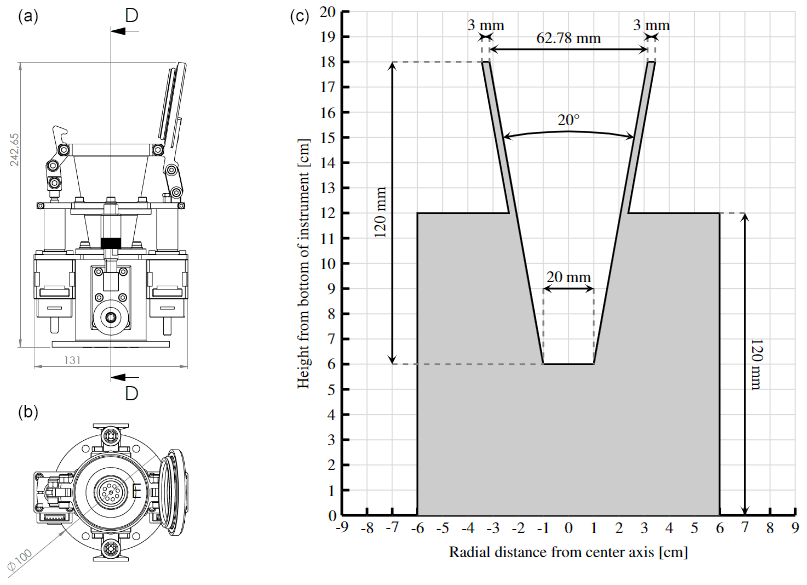
Figure 1 (a) Side view technical drawing of the MESS detector. (b) Top view technical drawing of the MESS detector. (c) Simplified drawing of the MESS detector used in the simulations.

3 Model description

In order to track the dust particles in the instrument, their trajectories are calculated by solving numerically the equation of motion for each dust particle. Accordingly, the modeling of the dust particle trajectories is presented in Sect. 3.1. As the motion of the dust particles is mainly driven by the drag force that the dust particles undergo, which depends on the characteristics of the background gas, i.e., the air in the upper atmosphere, Sect. 3.2 presents the evaluation of the flow of the air in the vicinity of the instrument. Finally, we assume here that the ice particles can break up when they collide with the funnel wall of the instrument, and the fragmentation modeling and underlying assumptions are introduced in Sect. 3.3. Regarding the MSPs, it is assumed that they do not fragment and that the collision of a MSP with the funnel wall results in a specular reflection.

3.1 Dust particle dynamics

Since both MSPs and ice particles are considered, the trajectories of both of them have to be calculated. Since the ice particles are mostly composed of ice and MSPs represent a small fraction, the bulk properties of the ice particles are determined from the ice characteristics. Note that it is assumed that ice particles contain 3 % of MSPs and 97 % of ice. We assume that the dust particles are perfectly spherical, with a radius r_d and a mass density ρ_d. This is in particular true if the radius of the dust particles is larger than about 1 nm. For smaller radius, the geometry of the dust particles needs to be considered, and the model presented in this section is no longer valid and cannot be used in that case. Then, the dust particles are assumed to be neutral; i.e., electric and magnetic effects can be neglected and only subjected to the drag force and gravity. The drag force comes from the collisions between the molecules of the background gas and the dust particles. It is incidentally assumed that the dust particles are by far more massive than the gas molecules. As a consequence, the dust particles are heated due to these collisions, and their temperature may reach the sublimation temperature. At this moment, the dust particles will start to sublimate, making it necessary to consider their mass variation. Note that sublimation is a priori more likely to take place for ice particles than for MSPs. Finally, by taking the rocket as the reference frame, the equation of motion of the dust particles having a velocity v_d reads (Baines et al., 1965; Smirnov et al., 2007; Antonsen and Havnes, 2015)

$$\begin{array}{}\text{(1)}& {\displaystyle \frac{\mathrm{d}{\mathit{v}}_{\mathrm{d}}}{\mathrm{d}t}}={\displaystyle \frac{\mathrm{1}}{m_{\mathrm{d}}}}\left[m_{\mathrm{d}}\mathit{g}+\mathit{\chi }\mathit{\pi }{r}_{\mathrm{d}}^{\mathrm{2}}{m}_{\mathrm{g}}{n}_{\mathrm{g}}{v}_{\text{th},\mathrm{g}}^{\mathrm{2}}f\left(u\right){\displaystyle \frac{{\mathit{v}}_{\mathrm{g}}-{\mathit{v}}_{\mathrm{d}}}{\left|{\mathit{v}}_{\mathrm{g}}-{\mathit{v}}_{\mathrm{d}}\right|}}-{\displaystyle \frac{\mathrm{d}{m}_{\mathrm{d}}}{\mathrm{d}t}}{\mathit{v}}_{\mathrm{d}}\right],\end{array}$$

with $m_{\mathrm{d}}=\mathrm{4}\mathit{\pi }{\mathit{\rho }}_{\mathrm{d}}{r}_{\mathrm{d}}^{\mathrm{3}}/\mathrm{3}$ the mass of the dust particles. In the right-hand side, the first term corresponds to gravity, with g the gravity acceleration; the second term corresponds to the drag force; and the third term corresponds to the mass variation of the dust particles. Regarding the drag force, the parameter χ is associated with the geometry of the dust particles; for spherical dust particles χ=1. m_g, n_g and v_th,g, respectively, correspond to the molecules mass, density and thermal speed of the background gas. The thermal speed is defined by $v_{\text{th},\mathrm{g}}=\sqrt{\mathrm{2}{k}_{\mathrm{B}}{T}_{\mathrm{g}}/m_{\mathrm{g}}}$, with k_B the Boltzmann constant as a function of the temperature of the background gas T_g. The function f is given by

$$\begin{array}{}\text{(2)}& f\left(u\right)={\displaystyle \frac{\mathrm{1}}{\sqrt{\mathit{\pi }}}}\left(u+{\displaystyle \frac{\mathrm{1}}{\mathrm{2}u}}\right)e^{-u^{\mathrm{2}}}+\left(\mathrm{1}+u^{\mathrm{2}}-{\displaystyle \frac{\mathrm{1}}{\mathrm{4}{u}^{\mathrm{2}}}}\right)\text{erf}\left(u\right)\end{array}$$

in terms of the relative speed $u=\mathrm{|}{\mathit{v}}_{\mathrm{g}}-{\mathit{v}}_{\mathrm{d}}\mathrm{|}/v_{\text{th},\mathrm{g}}$, assuming specular reflection of background gas molecules during collisions with dust particles. Note that such a modeling of the drag force is valid for both subsonic and supersonic regimes. Because of the heating of the dust particles that can be important enough to lead to the sublimation of the ice layer, the evolution of the dust particle temperature T_d has to be modeled. It is given by the energy balance that can be written as follows (Horányi et al., 1999; Antonsen and Havnes, 2015):

$$\begin{array}{}\text{(3)}& {\displaystyle \frac{\mathrm{d}{T}_{\mathrm{d}}}{\mathrm{d}t}}={\displaystyle \frac{\mathrm{1}}{m_{\mathrm{d}}{c}_{\mathrm{d}}}}\left({\displaystyle \frac{\mathit{\pi }}{\mathrm{4}}}{r}_{\mathrm{d}}^{\mathrm{2}}{n}_{\mathrm{g}}{v}_{\text{th},\mathrm{g}}{k}_{\mathrm{B}}{T}_{\mathrm{g}}g\left(u\right)-L_{\mathrm{d}}{\displaystyle \frac{\mathrm{d}{m}_{\mathrm{d}}}{\mathrm{d}t}}\right),\end{array}$$

with c_d and L_d the dust particle specific heat and latent heat, respectively. The first term of the right-hand side corresponds to the heating due to the collisions with background gas molecules, and the second corresponds to the modification of the internal energy due to the sublimation. Similarly to Eq. (2), the function g is defined as a function of the relative speed u and is given by

$$\begin{array}{}\text{(4)}& g\left(u\right)={\displaystyle \frac{\mathrm{2}}{\sqrt{\mathit{\pi }}}}(\mathrm{5}+\mathrm{2}{u}^{\mathrm{2}})e^{-u^{\mathrm{2}}}+{\displaystyle \frac{\mathrm{3}+\mathrm{12}{u}^{\mathrm{2}}+\mathrm{4}{u}^{\mathrm{4}}}{u}}\text{erf}\left(u\right),\end{array}$$

so that the modeling of the heating of the dust particles is valid for both subsonic and supersonic regimes. It can be pointed out that radiative processes, such as thermal emission of the dust particles, solar radiation and terrestrial radiation, are neglected in Eq. (3) (Rizk et al., 1991). The mass variation of the dust particles d_tm_d appearing in Eqs. (1) and (3) associated with the mass loss due to the sublimation corresponds to a flux of molecules constituting the dust particles out of their surface. Thus, the mass variation of the dust particles is defined by

$$\begin{array}{}\text{(5)}& {\displaystyle \frac{\mathrm{d}{m}_{\mathrm{d}}}{\mathrm{d}t}}=-\mathrm{4}\mathit{\pi }\mathit{\rho }{r}_{\mathrm{d}}^{\mathrm{2}}{\displaystyle \frac{\mathrm{d}{r}_{\mathrm{d}}}{\mathrm{d}t}},\end{array}$$

where the radius variation is evaluated by assuming that dust particle molecules leave the surface diffusively. It is given by the Hertz–Knudsen equation (Skorov and Rickman, 1995; Kossacki and Leliwa-Kopystynski, 2014; Antonsen and Havnes, 2015), which can be written as

$$\begin{array}{}\text{(6)}& {\displaystyle \frac{\mathrm{d}{r}_{\mathrm{d}}}{\mathrm{d}t}}=-{\displaystyle \frac{P_{\text{vap}}}{{\mathit{\rho }}_{\mathrm{d}}}}\sqrt{{\displaystyle \frac{m_{\mathrm{D}}}{\mathrm{2}\mathit{\pi }{k}_{\mathrm{B}}{T}_{\mathrm{d}}}}},\end{array}$$

with m_D the mean mass of dust particles. P_vap corresponds to the vapor pressure and is given by (Podolak et al., 1988)

$$\begin{array}{}\text{(7)}& P_{\text{vap}}=P_{\mathrm{0}}\exp \left(-{\displaystyle \frac{T_{\mathrm{0}}}{T_{\mathrm{d}}}}+{\displaystyle \frac{\mathrm{2}{\mathit{\gamma }}_{\mathrm{d}}{m}_{\mathrm{D}}}{\mathit{\rho }{r}_{\mathrm{d}}{k}_{\mathrm{B}}{T}_{\mathrm{d}}}}\right),\end{array}$$

where P₀ and T₀ are constants depending on the type of dust particles, i.e., ice particles or MSPs. The second term in the exponential corresponds to a correction of the vapor pressure so that spherical mass ejection for very small surfaces is considered (Evans, 1994). This correction term is given in terms of the specific surface energy γ_d of the dust particles.

3.2 Airflow model

In order to calculate the trajectories and the heating of the dust particles, the number density, the temperature and the velocity of the background gas have to be evaluated. Such an evaluation is done by using the DS2V program developed by Bird and Brady (1994). It is 2D numerical software based on direct simulation Monte Carlo (DSMC) methods which are commonly used to study rarefied gas dynamics. The mesosphere and the lower thermosphere are characterized by a Knudsen number usually between 0.01 and 1 for standard size of instrument collecting mesospheric dust particles, which corresponds to a rarefied gas (Antonsen and Havnes, 2015). The Navier–Stokes equations which are suitable for a continuous flow (when Kn ≪ 0.1) cannot be used anymore, and probabilistic methods should be preferred.

3.3 Fragmentation model

Because of the conical shape of the detector, a large number of the incoming dust particles can collide with the funnel walls. We assume that during the collision, MSPs are reflected without breaking up while the ice particles can break into fragments. Little is known of this fragmentation process, and we refer to results obtained from ice collision experiments and molecular simulations (Tomsic et al., 2003). It was found that a large fragment is likely to be created during the collision of pure ice particles onto a metal wall with a large angle with respect to the normal direction of the surface. Accordingly, it is assumed for our case that a large fragment is created having a mass equal to half of the mass of the incoming ice particle and the same composition as the incoming ice particle, i.e., 3 % of MSPs and 97 % of ice. The other half of the mass is divided between a large number of smaller fragments. They are assumed to be small enough that the ice sublimates immediately. According to the mass conservation and by assuming that the radius distribution ω(r) the MSP fragments scale as $\mathit{\omega }\left(r\right)\propto r^{-\mathrm{3}}$ supported by results from in situ measurements (Antonsen et al., 2020), it can be deduced that the mean radius of these fragments is mostly smaller than 0.8 nm; see Appendix A. This means that the model presented in the previous section is no longer suitable and cannot track the MSP fragments. Finally, the description of the fragmentation process that is used in this work to investigate the trajectories of the MSP fragments is summarized in Fig. 2. We consider only the large fragment if r_d < 6 nm right before the collision, and we consider the large fragment plus one MSP fragment having a radius of 1 nm if r_d > 6 nm right before the collision. For both the large fragment and the MSP fragment, it is assumed that the angle after collision is the same as the angle of the incident ice particle due to specular reflection.

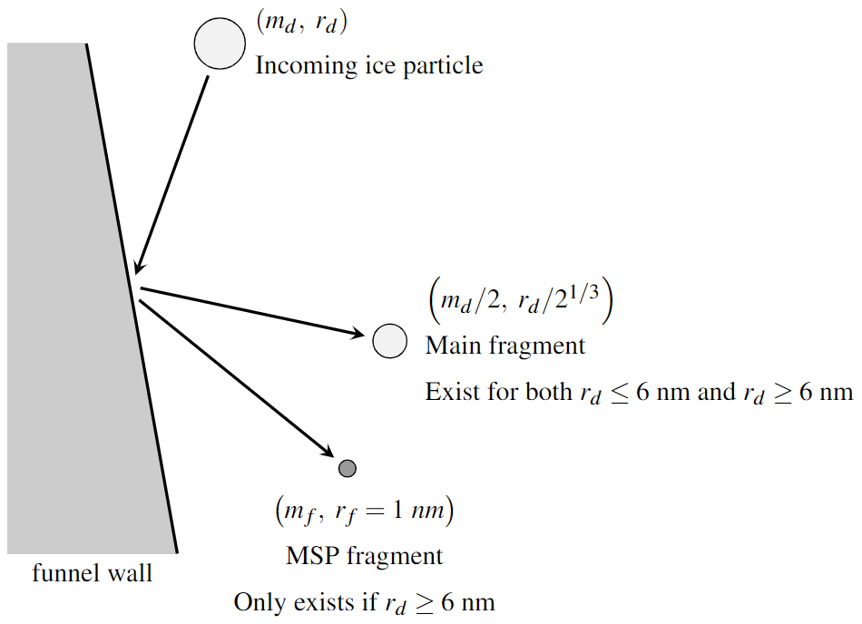
Figure 2 Drawing of the modeling of the ice particle fragmentation process having a mass m_d and a radius r_d when they collide with the funnel wall. The size scales are not respected for the sake of clarity. When r_d > 6 nm, the angle associated with the two fragments is the same as the angle of the incident particle with respect to normal direction of the surface. Different angles are displayed for the sake of clarity.

Another kind of collision happens when the mesospheric dust particles hit the top of the funnel or the collection area. In those cases, the collision is head-on and the model we just described is not suitable. For head-on collisions of ice particles, it is assumed that the ice particles entirely break up where the ice vaporizes, and the MSPs are released because the speed of the ice particle during the collision is about several hundreds of meters per second. For head-on collisions of MSPs, it is assumed that the MSPs rebound without being destroyed.

4 Results

This section is dedicated to the presentation of the results coming from simulations performed for different altitudes and different rocket speeds.The altitudes of 80, 82, 85 and 90 km are considered as they correspond to the borders and centers of the region of interest as mentioned in Sect. 1. The rocket velocity varies with the altitude and depends on the rocket apogee. For a mesospheric rocket, the apogee lies between 110 and 130 km, and a speed of around 1000 m s⁻¹ at an altitude between 80 and 90 km can be expected. Accordingly, rocket speeds of 800, 1000 and 1200 m s⁻¹ are considered. It can be pointed out that such speeds are associated with supersonic flows. The airflow of the background gas in the vicinity of the instrument is first presented in Sect. 4.1. Then, the trajectories of dust particles are presented in Sect. 4.2 with two illustrative examples. In order to evaluate in a more comprehensive way the dust particle motion in the instrument, the detection rates are presented in Sect. 4.3 for the different altitudes, different rocket velocities and different dust particle initial radii. These detection rates are then used to estimate the mass of dust particles collected during a rocket flight. Finally, the final temperatures and speeds of the dust particles when they reach the collection area are presented in Sects. 4.4 and 4.5, respectively.

4.1 Neutral gas flow

The flow of the background gas around the rocket depends on its density and temperature. These parameters, and in particular the density, can vary over short spatial and temporal scales. Variations by roughly a factor of 2 were observed for the density during previous rocket campaigns (Lübken et al., 1993; Strelnikov et al., 2003). However, such variations are neglected in a first approximation and because it is out of the scope of the present work. Thus, mean values provided by the NRLMSISE-00 atmospheric model are used to evaluate the initial densities and temperatures of the background gas (NRL, 2024; Picone et al., 2002). The model has been used to look at the data in July at a place of GPS coordinates 69° N, 16° E, in order to estimate the atmospheric conditions in the summer near the Andøya Space Center. These values are gathered in the Table 1 for the four different altitudes.

Table 1 Initial densities and temperatures of the background gas for the four different altitudes coming from the NRLMSISE-00 atmospheric model (NRL, 2024; Picone et al., 2002).

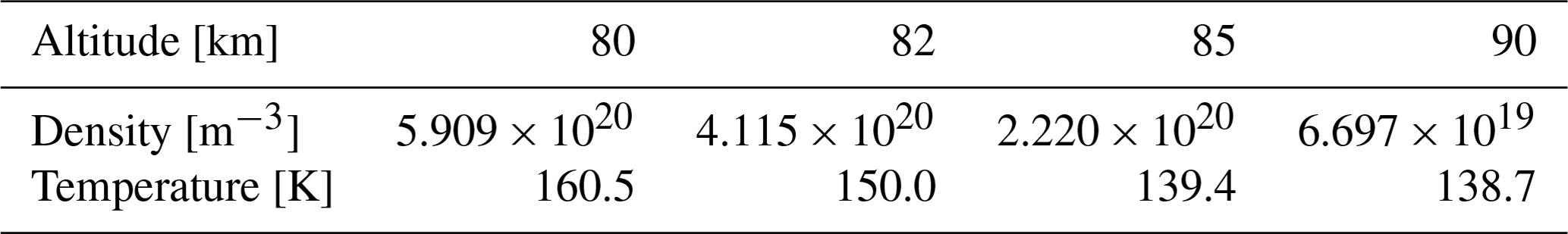
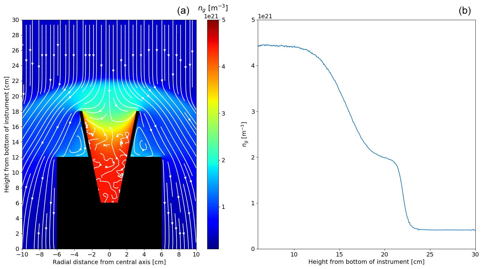
Figure 3 Results of the DSMC simulations showing (a) the background gas density n_g and stream around the detector and (b) a lineout of the background gas density n_g with respect to the height from the bottom of the detector for an altitude of 82 km and a rocket speed of 1000 m s⁻¹.

Figure 3 shows the airflow and the gas density around the instrument at an altitude of 82 km and rocket speed of 1000 m s⁻¹. The airflows associated with the other altitudes and rocket speeds are in Appendix B since they are relatively similar to the one shown in Fig. 3. It can be seen that a bow shock with a thickness of about 4 cm is created at the top of the detector. This is because the rocket speed is always higher than the sound speed of the background gas. The gas density in the bow shock is higher than the initial density by a factor of 3 to 4 depending on the rocket speed. Below the bow shock, the gas density reaches its highest value in the funnel, where it is higher than the initial density by about 1 order of magnitude depending on the rocket speed. The increase in the gas density in these two regions implies that the dust particles can be slowed down by undergoing the drag force twice, first during the bow shock crossing and then, and in a more important way, when being inside the funnel. Finally, it can be observed that the stream is mainly laminar around the detector but becomes turbulent inside the detector, which means that the trajectories of the dust particles may be modified because of this turbulence. Given the slowdown that dust particles can experience when crossing the bow shock or being in the funnel and given the turbulence taking place in the detector, it can be expected that a significant fraction of the small particles do not reach the collector. When looking at the influence of the rocket speed on the gas density for a given altitude, it appears that the gas density of the bow shock and inside the detector increases with the rocket speed, which means that a higher rocket speed leads to a stronger drag force. Thus, increasing the rocket speed does not necessarily entail a more efficient collection of dust particles as they would be influenced more importantly by the drag force and possibly decelerated more than for a lower rocket speed. This is addressed in Sect. 4.3.

4.2 Dust particle trajectories

The previous results providing the airflow of the background gas in the vicinity of the instrument can now be used to evaluate the motion of the dust particles. To do so, Eqs. (1)–(6) are solved numerically using the fourth-order Runge–Kutta method. These equations are function of the mass density ρ_d, the specific heat c_d, the latent heat L_d, the mean mass m_D, the specific surface energy γ_d, and the parameters P₀ and T₀ of dust particles that are different for ice particles and MSPs. The values of these parameters are gathered in Table 2 for both ice particles and MSPs (Podolak et al., 1988; Antonsen and Havnes, 2015). The particle tracking in the simulation is stopped either when the particle reaches the detector or when the particle is no longer in the simulation box (i.e., the particle is taken away from the instrument by the airflow and does not reach the detector); when the particle is stopped due to the slowing down coming from the drag force (i.e., the particle does not reach the detector); or, for ice particles, when the particle radius becomes smaller than 0.8 nm where the model is no longer valid. In that case, the particle does not reach the detector because it is completely sublimated. This section aims at presenting the results obtained from these simulations for both ice particles and MSPs through the evaluation of their trajectories. For the sake of clarity, it has been chosen to present only one representative example for both ice particles and MSPs showing the typical trajectories of the dust particles in the instrument instead of an exhaustive list. To investigate the trajectories of the dust particles in a comprehensive way, the evaluation of the trajectories should be done for different altitudes, different rocket velocities and different initial radius, leading to the very large number of cases. The presentation in the next section of the collection rates as a function of these parameters aims at addressing this question and studies the efficiency of the instrument for different altitude and rocket speeds.

Table 2 Values of the mass density ρ_d, the specific heat c_d, the latent heat L_d, the mean mass m_D, the specific surface energy γ_d, and the parameters P₀ and T₀ for ice particles and MSPs. It is reminded here that P₀ and T₀ do not represent the pressure or the temperature of any dust particles, but they are constants that have the dimension of a pressure and a temperature. Note that for the ice particles, the specific heat is expressed in terms of the ice particle temperature T_d.

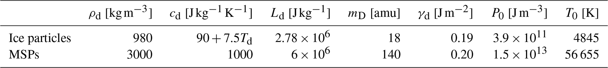
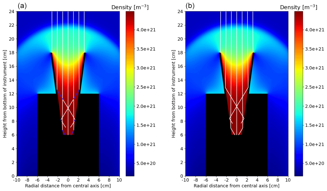
Figure 4 Trajectories of ice particles and MSPs in the MESS instrument for rocket velocity of 1000 m s⁻¹ and an altitude of 82 km. (a) Ice particles with an initial radius of 13 nm. The white lines represent the ice particle trajectories. The blue lines represent the trajectories of the fragments constituted of pure MSPs created during each collision of an ice particle with a funnel wall. (b) MSPs with an initial radius of 7 nm.

Instead of giving an extensive list of trajectories for different altitudes, different rocket speeds and different initial radius, we prefer instead to show an illustrative case gathering the different trajectories that can be exhibited by the dust particles when they cross the instrument. The dependence of the trajectories on the altitude, the rocket speed and the initial radius of the dust particle is discussed in the next section by looking at the collection rates. Accordingly, Fig. 4 shows the trajectories of ice particles that have an initial radius of 13 nm and the trajectories of MSPs that have an initial radius of 7 nm. In both cases, a rocket velocity of 1000 m s⁻¹ and an altitude of 82 km are considered. Different trajectories can be identified. First, dust particles starting near the central axis of the instrument are identified. It can be seen that an ice particle with an initial radius of 13 nm and a MSP with an initial radius of 7 nm entirely cross the instrument and reach the collection area. However, if some dust particles are smaller and lighter, they are likely not to reach the collection area. They are slowed down because of the drag force and will eventually float in the instrument. This leads to a sort of threshold initial radius for the dust particles above which they should always reach the collection area. The largest value for this threshold initial radius is reached for a rocket speed of 1200 m s⁻¹ and an altitude of 80 km corresponding to the highest rocket speed and the lowest altitude, with this case being associated with the most important increase in the gas density in the bow shock and in the funnel. In that case, the minimum initial radius is about 11 nm for ice particles and is about 9 nm for MSPs. Then, dust particles starting a bit farther from the central axis are identified. They enter the instrument and, if they are large enough, collide with the funnel wall; otherwise, they are progressively stopped by being slowed down due to the drag force. This corresponds to the trajectories ending in the middle of the instrument. This is further investigated in Sect. 4.5 dealing with the final speeds of the mesospheric dust particles. In the case of an ice particle, the collision leads to a rebound during which the radius of the ice particle is divided by a factor of ${\mathrm{2}}^{\mathrm{1}/\mathrm{3}}$ and a formation of a fragment constituted of pure MSPs. In the case of a MSP, the collision only leads to a rebound. In both cases, starting relatively far from the central axis means that dust particles can bounce several times and travel over a larger distance than a dust particle starting near the central axis. They undergo the influence of the drag force during a longer time and are slowed down more. Moreover, ice particles colliding several times see their radius divided by a factor of ${\mathrm{2}}^{\mathrm{1}/\mathrm{3}}$ at each collision, become smaller and are slowed down more importantly by the drag force. Therefore, it is possible that they do not reach the collection area. In addition, fragments resulting from the collision of an ice particle with a funnel wall are quickly slowed down because they are very small, ∼ 1 nm, and only those created near the collection area are likely to reach it. If the fragments are created far from the collection area, they will float in the instrument after being entirely slowed down. Finally, dust particles starting far from central axis of the instrument are identified. These particles cannot be collected since they either are taken away by the airflow or hit the top of the funnel. For ice particles in that case, they will explode in a large number of small fragments. Unlike the collisions that are considered in the fragmentation process presented in Sect. 3.3, the collision here is head-on and any large fragment is created. All of the fragments are small and are taken away by the airflow, even those heading toward the central axis of the instrument, because of the stream existing in that region; see Figs. B1 to B4.

In Fig. 4, it can be seen that the trajectories of the particles entering the instrument either reach the collection area or end somewhere inside the instrument. This is a result of the deceleration, which can cause some particles to float inside the instrument. The case where particles enter the instrument and then go out by being taken away by the airflow, as it could have been expected when looking at the streams, especially in Figs. B1 and B2, does not happen, except for small fragments created by head-on collision on the top of the funnel wall. In addition, it was observed by looking at the airflow streams that turbulence takes place in the instrument. It appears that this turbulence does not have any influence of the dust particle trajectories. These conclusions are drawn by evaluating the trajectories of ice particles and MSPs having an initial radius of 13 and 7 nm, respectively. However, they can be generalized to other radius. Even though trajectories of dust particles having a different initial radii are not shown here for the sake of clarity, a large number of simulations have been performed to evaluate the trajectories of dust particles that have an initial radius ranging from 1 to 20 nm for ice particles and ranging from 1 to 10 nm for MSPs. The simulations are then used to evaluate to the collection efficiency of the instrument for different altitudes, different rocket speeds and different initial radius for the dust particles.

4.3 Collection rates

It is observed in the last section that when entering the instrument, some of the dust particles can reach the bottom of the instrument and be collected but others are sufficiently slowed down to be completely stopped and eventually float in the instrument. This section is dedicated to the presentation of the collection rates of the ice particles and MSPs reaching the collection area. These rates are obtained by calculating the ratio between the number of particles reaching the collection area and the number of particles entering the instrument. The rates are calculated for different initial radius for the dust particles, different rocket speeds and different altitudes. In each case, about 150 dust particles are considered as a compromise between a number that is large enough to be relevant for statistics and a number not too large regarding computational capabilities.

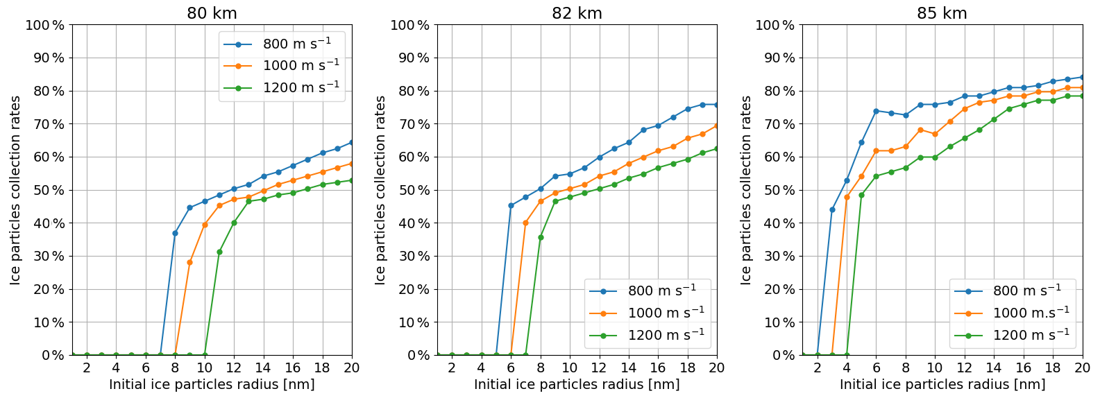
Figure 5 Ice particle collection rates as a function of their initial radius for three different rocket speeds (800, 1000 and 1200 m s⁻¹) and three different altitudes (80, 82 and 85 km). Each point of the graphs has been obtained by calculating the trajectories of about 150 ice particles.

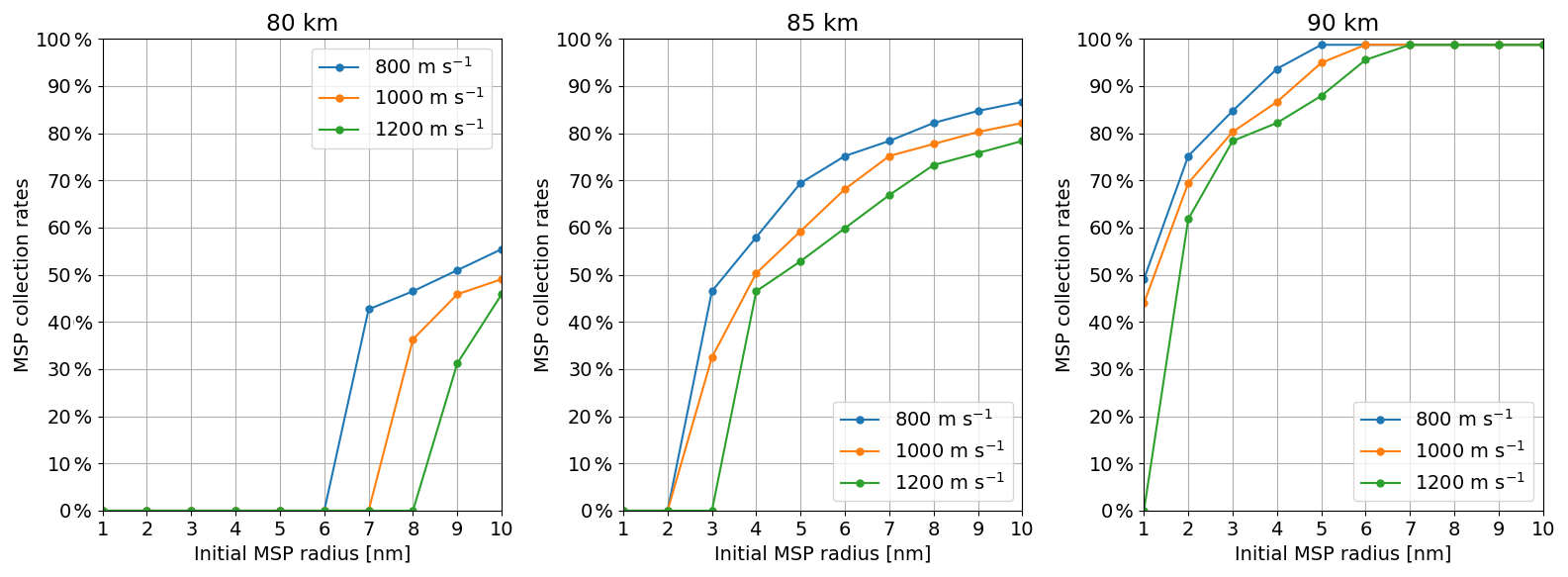
Figure 6 MSP collection rates as a function of their initial radius for three different rocket speeds (800, 1000 and 1200 m s⁻¹) and three different altitudes (80, 85 and 90 km). Each point of the graphs has been obtained by calculating the trajectories of about 150 MSPs.

Figure 5 shows the collection rates of ice particles as a function of their initial radius. They are shown for different rocket speeds (800, 1000 and 1200 m s⁻¹) and different altitudes (80, 82 and 85 km). As mentioned in Sect. 1, most of the ice particles are located between 80 and 85 km with a peak around 82 km. Similarly, Fig. 6 shows the collection rates of MSPs as a function of their initial radius. They are also shown for different rocket speed (800, 1000 and 1200 m s⁻¹), as for ice particles, and different altitudes (80, 85 and 90 km), which are different for the altitudes considered for ice particles. As seen in Sect. 1, most of the MSPs are located between 80 and 90 km with a peak around 85 km. Overall conclusions are basically the same for both ice particles and MSPs. First, it can be observed that the collection rates increase with the initial radius. Larger dust particles are more likely to reach the collection area as their trajectories are less influenced by the drag force. Then it can be seen that the collection rates are more important for higher altitudes and lower rocket speed. At higher altitudes, the density of the background gas is smaller, leading to a weaker drag force; this can be assumed to be proportional to the background density in a first approximation (see Sect. 3.1), and a larger number of particles are likely to reach the collection area. Similarly, it appears that a slower rocket leads to a more efficient collection of ice particles. One might expect that a higher rocket speed would result in better collection because the dust particles pass through the bow shock and the instrument faster and are exposed to the drag force for a shorter period of time. On the contrary, we find that the higher drag force at higher rocket speed reduces the collection rate. This answers the question on the competition between drag force and initial particle speed raised in Sect. 4.1. Finally, it can be observed that particles smaller than a certain size do not reach the collection area. This creates a sort of threshold radius ranging from 2 to 10 nm for ice particles and from 1 to 8 nm for MSPs depending on the rocket speed and altitude. A lower rocket speed or a rocket flight at a lower altitude leads to a weaker drag force, allowing smaller particles to reach the collection area. Such an effect may have to be considered during the design of the rocket mission with respect to the apogee. Those particles having a radius smaller than the threshold radius are slowed down and stopped in the instrument and eventually float. Even if these particles do not reach the collection area, they could still be collected when the closing system is activated as they would remain inside the instrument. Thus, the instrument will have to be opened carefully during the sample analysis so that there is no loss of the these potential particles floating in the instrument. In addition, the walls of the funnel should be inspected as dust particles could be stuck on them. Overall, it appears that the MESS instrument presented in this work can collect dust particles over a large range of size. This instrument should efficiently collect ice particles larger than 10 nm and MSPs larger than 8 nm. In addition, it should be able to collect a significant number of ice particles larger than 2 nm and MSPs larger than 1 nm, even though the collection rates are the most important at the highest altitude where dust particles are less numerous (Megner et al., 2006; Baumann et al., 2013).

4.4 Estimate of the final temperatures

During their entry in the instrument, dust particles can be heated until undergoing mass loss when they start to sublimate. This heating that cannot be avoided with the current rocket speed may lead to modification of the chemical composition of the dust particles which would complicate the laboratory analysis. This section aims at addressing this question by looking at the final temperature of the dust particles, i.e., the temperature of the dust particles when they reach the collection area.

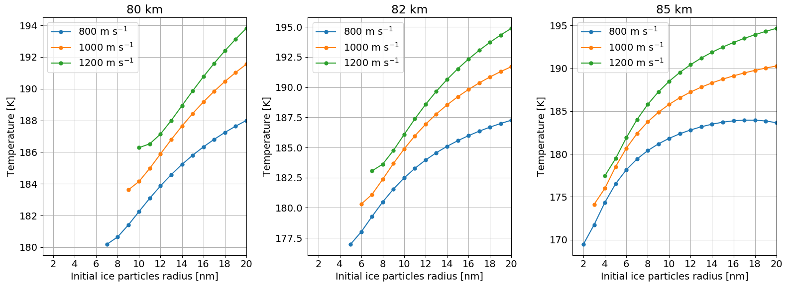
Figure 7 Evolution of the final temperatures of the ice particles, i.e., when they reach the collection area, with respect to the initial radius for different rocket velocities and different altitudes.

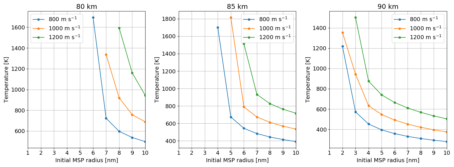
Figure 8 Evolution of the final temperatures of the MSPs, i.e., when they reach the collection area, with respect to the initial radius for different rocket velocities and different altitudes.

Figures 7 and 8 show the final temperatures of ice particles and MSPs, respectively, as a function of their initial radius for the three rocket speeds (800, 1000 and 1200 m s⁻¹) and different altitudes. Similarly to the previous section, the final temperatures of ice particles are shown for an altitude of 80, 82 and 85 km, and the final temperatures of MSPs are shown for an altitude of 80, 85 and 90 km. The particles that are considered here are those starting in the central axis of the instrument for the purpose of illustration. It has been checked that there are no relevant variations for the final temperatures depending on the initial position of the dust particles. In addition, ice particles starting at the center are those that are heated the most, which should provide the upper limit of the final temperatures. It can be seen for ice particles that there is no drastic change for the final temperatures. The largest difference is about 25 K overall between 170 and 195 K. The heating due to the drag force leads to a melting of the outer surface of the ice particles that remains relatively cold. The fact that the final temperature ranges from 170 to 190 K also means that crossing the instrument results in a relatively small increase in their temperature. It is about a few tens of kelvins since the initial temperature of the dust particles is between about 140 and 160 K; see Sect. 4.1. This means that the MSPs located inside the ice particles are not significantly heated during their collection, and the ice can be considered as acting like a thermal shield. Finally, the trends with respect to the rocket speed and the altitude are once again due to the drag force. A lower altitude and a faster rocket are associated with a stronger drag force, resulting in a more important heating. Concerning pure MSPs, it can be seen they are heated significantly, up to 1800 K. Although the first term in Eq. (3) associated the heating induced by the drag force is about the same order of magnitude for MSPs and ice particles, the second term associated with the mass variation is much smaller for MSPs than for ice particles. The parameter T₀ taking part of the expression of the vapor pressure that is used to evaluate the mass variation is very different between MSPs and ice particles. One has T₀ = 56 655 K for MSPs and T₀ = 4845 K for ice particles, leading to a difference by a factor about 10. Thus, for MSPs, the heating is not counterbalanced by the mass variation, and MSPs can reach high temperatures. Said differently, this can be interpreted by the fact that the melting temperature of the MSPs is much higher than the melting temperature of the ice. Since the temperature increases up to the melting temperature, the MSPs have a much higher temperature than the ice particles. In both cases, the high temperature for the MSPs means that their chemical composition can be altered during their crossing of the instrument, and the chemical composition of MSPs reaching the collection can be different from the chemical composition of MSPs before they enter the instrument, i.e., when they are present in the mesosphere. Finally, it appears that a slower rocket and a higher altitude lead to a final temperature that is significantly lower. This can thus be an additional reason to prefer slower rockets as they are less likely to induce a change in the chemical composition of MSPs.

4.5 Estimate of the final speeds

When reaching the collection area, the dust particles have a nonzero speed. Depending on that speed, the dust particles may damage the TEM grids, the walls of the collection area and the instrument more generally. Additionally, they may also break up when eventually hitting the collection area or bouncing off. This section aims at addressing this question by looking at the final speed of the dust particles.

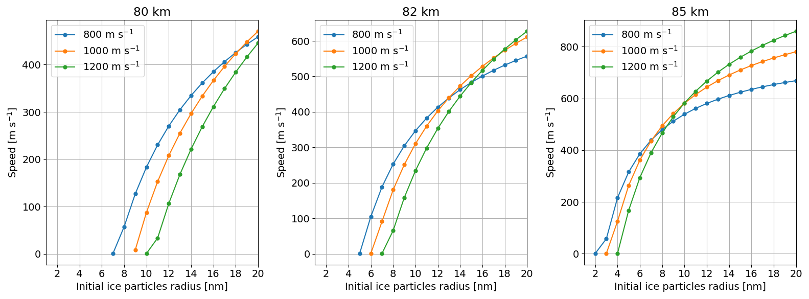
Figure 9 Evolution of the final speeds of the ice particles, i.e., when they reach the collection area, with respect to the initial radius for different rocket speeds and different altitudes.

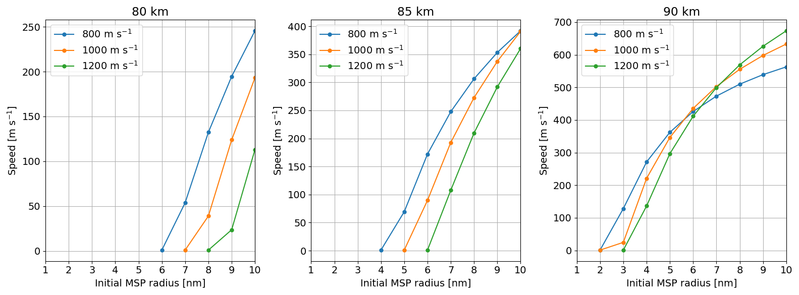
Figure 10 Evolution of the final speeds of the MSPs, i.e., when they reach the collection area, with respect to the initial radius for different rocket speeds and different altitudes.

Figures 9 and 10, respectively, show the final speeds of the ice particles and MSPs as a function of their initial radius, for the same rocket speeds and altitudes as previously. We can see that the final speed of the ice particles and MSPs quickly increases, and most of the dust particles have a final speed of several hundreds of meters per second. For low altitude, it can be seen that a slower rocket leads to a higher final speed for the dust particles. Said differently, a faster rocket leads to a more efficient deceleration of the dust particles, which comes from the bow shock created by the rocket that is strong enough to slow down the dust particles efficiently. At higher altitudes, a slower rocket leads on the contrary to lower final speeds. In that case, the density of the atmosphere is such that the bow shock created by the rocket is not strong enough to slow down larger dust particles. Then, the final speed is driven by the rocket speed. In contrast to the last section where it clearly appears that slower rockets would be more beneficial, the situation seems more ambiguous here. A slower rocket would be more beneficial at higher altitude but a faster rocket would be more beneficial at lower altitude. However, for all the rocket speeds, the number of dust particles bouncing off should be very small because most of them have a final speed higher than 100 m s⁻¹. Although the impact of nanometer-sized particles on carbon foils has not been studied to the best of our knowledge, the collision of larger aggregate particles has been both theoretically and experimentally investigated during the evaluation of the particle growth in protoplanetary disks. It was found that bouncing happens for collision speeds smaller than 10 m s⁻¹ for particles with the same material (Blum and Wurm, 2008; Wada et al., 2011). Bouncing is prevented when the kinetic energy of the impacting particle is immediately transferred to the target. We expect that this is the case at the collection grids, where the particles hit a carbon foil. The film has a relatively low material strength, and the particles would rather penetrate the foil due to head-on collisions.

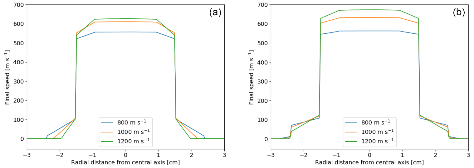
Figure 11 Profiles of the final speed of ice particles and MSPs along the radial dimension for three different rocket speeds. (a) Radial profiles of the final speed of ice particles associated with an altitude of 82 km and an initial radius of 20 nm. (b) Radial profiles of the final speed of MSPs associated with an altitude of 85 km and an initial radius of 10 nm.​​​​​​​

It can be pointed out that Figs. 9 and 10 show the final speeds of dust particles starting in the central axis of the instrument. Unlike the final temperatures, the final speed of the dust particles strongly depends on their initial position with respect to the central axis. Accordingly, Fig. 11, respectively, show the profile of the final speeds of ice particles and MSPs with respect to the radial direction. For ice particles, these radial profiles are shown for an altitude of 82 km and an initial radius of 20 nm. For MSPs, the radial profiles are shown for an altitude of 85 km and an initial radius of 10 nm. In both cases, they are shown for the three rocket speeds (800, 1000 and 1200 m s⁻¹). It has been chosen to show the profiles associated with only one altitude and one initial size as a purpose of illustration. The altitudes of 82 and 85 km have been chosen as a mean altitude. The initial radii of 20 and 10 nm have been chosen because they correspond to the maximum radii which are considered in this work. Such dust particles should be the least decelerated, leading the upper limit of the final speed. It can be seen that the incoming dust particles near the central axis have the highest final speed. On the contrary, the incoming dust particles relatively far from the central axis have a much smaller final speed. This is due to the collision of the dust particles on the funnel wall. As a result of the collision, the dust particles have a much larger transverse speed and become more sensitive to the turbulence taking place in the instrument (see Sect. 4.1), leading to a deceleration of the dust particles.

4.6 Estimate of collected mass

We now estimate the total mass of mesospheric dust particles, i.e., MSPs, collected with the MESS instrument, although the numbers are subject to great uncertainty. Our assumptions are for conditions during the summer near Andøya since this corresponds to the time and location of a future experimental campaign. We first estimate the amount of MSPs contained in the ice particles that reach the detector. We then estimate the amount of MSPs that is collected directly and is not contained in the ice.

In contrast to previous experiments, MESS aims at collecting the dust material contained in ice particles. We base our estimate for this collection on the number densities in NLCs, which represent the large ice particles and their observations at the Andøya rocket launch site. The particle densities are from a study (Kiliani et al., 2015) based on several years of UV, VIS and IR lidar observations (Baumgarten et al., 2007, 2010) and with size distributions obtained from models (Berger and Lübken, 2015). For a given dust number density, the mass of collected particles m_collected is evaluated by

$$\begin{array}{}\text{(8)}& m_{\text{collected}}=A_{\text{coll}}\mathrm{\Delta }h{n}_{\mathrm{d}}{V}_{\text{dust}}{\mathit{\rho }}_{\mathrm{d},\text{msp}}\mathit{\alpha }\mathit{\sigma },\end{array}$$

where A_coll, Δh, n_d and ρ_d,msp are the collection area, the sample altitude, the dust particle number density and the mass density of MSPs, respectively. The dust volume V_dust is calculated from the radius r_d by assuming spherical particles. We investigated the collection efficiency, σ, above. The filling factor α denotes the mass fraction of the particle that consists of MSPs; we assume α=0.03. With these assumptions, we find that the mass of MSPs collected in ice particles amounts to 0.9620  10 × 10¹⁶, 1.001  10 × 10¹⁶, and 1.042  10 × 10¹⁶ amu for the rocket velocities 800, 1000 and 1200 m s⁻¹, respectively. This corresponds to a MSP deposition at the collection area around 3 × 10¹³ amu mm⁻² for a filling factor of 0.03 particle. With filling factors between 0.001 and 0.1, the deposited MSPs are ∼ × 10¹²–10¹⁴ amu mm⁻². These values are based on NLC observations near the Andøya rocket range. For comparison, a numerical global model study of polar mesospheric clouds (Yu et al., 2023) assumes for the water ice particles an average column ice content of the order of 400 µg m⁻². This latter value would correspond, for filling factor 0.03, to a MSP collection of 7×10¹² amu mm⁻², which is in the range of our estimate.

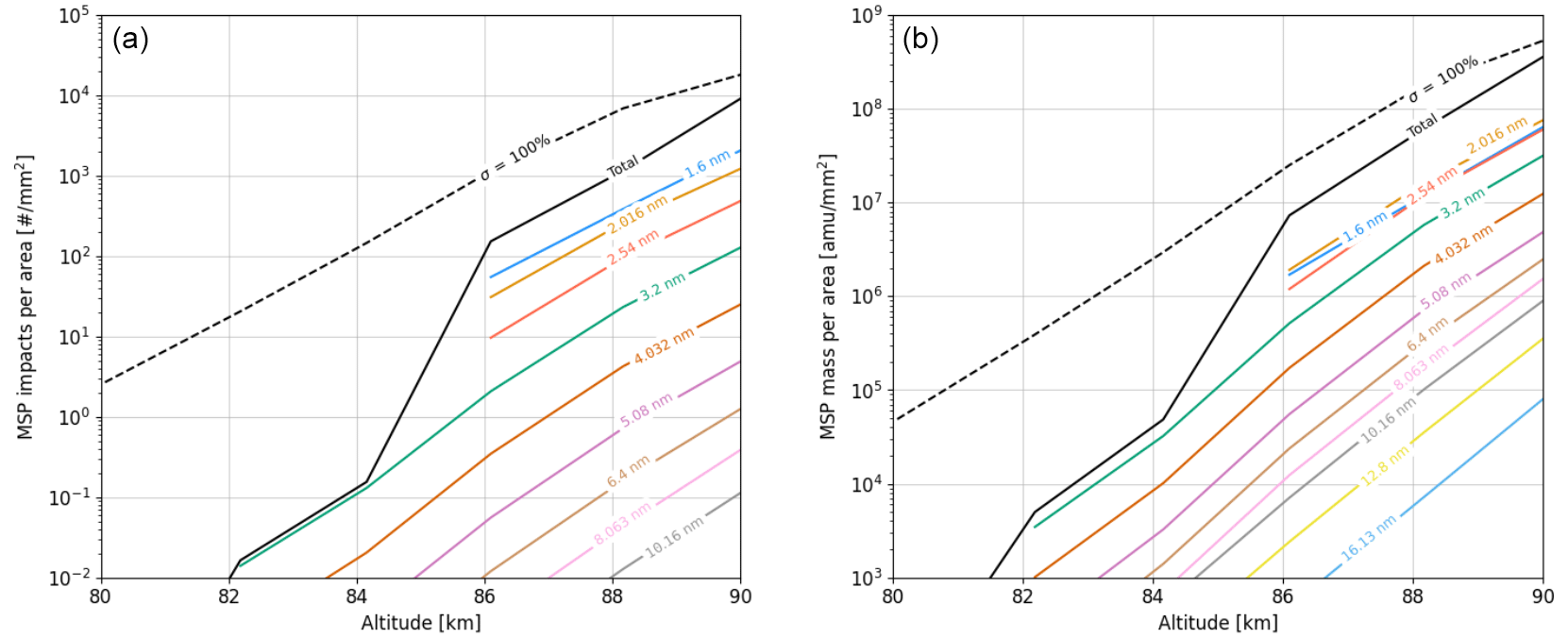
Figure 12 Elevation profiles for estimates of the cumulative amount of directly sampled MSPs reaching the detection surface, with a sampling area from 80 to 90 km and a rocket speed of 1000 m s⁻¹. The labels indicates the MSP size bin, and the black line shows the combined values for all size bins. Similarly the dashed black line shows total value, but with a collection efficiency fixed at 100 % at all altitudes. (a) Elevation profile of the cumulative number of directly sampled MSPs per detection surface area. (b) Elevation profile of the cumulative mass of directly sampled MSPs per detection surface area.

To estimate the MSPs that are directly collected, we rely on a global model, in particular for results from a model run of WACCM/CARMA carried out by W. Feng at the University of Leeds, UK. The results of this model run were applied in a recent study of the D-region incoherent scatter spectrum by Gunnarsdottir et al. (2023), and a further description can be found there. WACCM, the Whole Atmosphere Community Climate Model (Hervig et al., 2017), in combination with CARMA, the Community Aerosol and Radiation Model for Atmospheres (Bardeen et al., 2008), are used to simulate the growth, sedimentation and transport of meteor ablation products. The simulation run uses model parameters described in Brooke et al. (2017) – a meteoric influx of 7.9 t d⁻¹ and meteoric material density of 2 g cm⁻³ – and covers a 22-year period. It provides monthly averaged height profiles of the MSPs in 28 size bins ranging from 0.2 to 102.4 nm. However, particles larger than ∼ 10 nm have negligible number densities at mesosphere heights. The model results show little variation after 1 to 2 years (Gunnarsdottir et al., 2023; Greaker, 2023), and the results for the months June, July and August are similar. We combine the average dust number densities for the month of June and the collection efficiencies of MESS presented in this work to calculate the cumulative number of impacts and MSP mass per surface area at the MESS instrument. The values for June conditions and a rocket speed of 1000 m s⁻¹ are shown in Fig. 12. The values were derived according to Greaker (2023). The same work showed that by extending the sampling area to 95 km the amount of directly collected MSPs increases further to 10⁵ mm⁻². As such, it could prove beneficial to sample a larger area, in an attempt increase the amount of collected MSPs. We note that the used MSP number densities are small in comparison to other WACCM/CARMA model runs. This is partly, but not only, due to the meteorite influx assumed in the model run, which is relatively small. Higher meteorite influx can lead to higher number densities of MSPs, but the relationship is not linear (Bardeen et al., 2008).

5 Conclusions

Our calculations suggest that the MESS design for collecting dust particles during a rocket flight through a PMSE layer can return refractory MSP material of the order of 10¹⁶ amu, assuming that the rocket samples a 0.5–4 km height interval of PMSEs and that the collected ice particles contain a 3 % volume fraction of refractory MSPs. We estimate the range of the deposited MSPs at the sample collecting surface is ∼ × 10¹²–10¹⁴ amu mm⁻². It is found that the MESS instrument can efficiently collect both MSPs and ice particles with an initial radius of order of magnitude of 10 nm, and at heights above 85 km also smaller particles can be collected. While MSPs that are directly collected can reach temperatures higher than 1000 K due to heating induced by the drag force, ice particle temperatures remain lower than 200 K, and the chemical composition of the MSPs embedded in those ice particles is unchanged. Our calculations are based on model assumptions on the fragmentation at the funnel wall. We did not consider the cases where particles can stick to the funnel surface, nor did we consider charge effects. Dust particles can carry an initial charge and can also be charged during fragmentation. Including charged dust particles could result in an enhanced sticking to the walls and changes in the particle trajectory. In addition, the rocket payloads tend to become charged in their trajectory through the ionosphere. However, it has been shown that this charging in the mesosphere is small (Lai, 2011).

A further unknown is the orientation of the instrument and the rocket with respect to the flight direction, i.e., the angle of attack. Our calculations and estimations have been made by assuming a normal incidence corresponding to a zero angle of attack and the best-case scenario. However, an angle of attack cannot be avoided during the flight of sounding rockets. When the rocket is titled, the airflow and the flux of dust particles through the instrument are modified as well as the fragmentation process since the hypothesis of the large angle of incidence is no longer valid; see Sect. 3.3. We expect that an angle of attack of a few degrees may lead to modifications that lie within the uncertainties due to model assumptions. When modeling the case of a larger angle of attack, it becomes necessary to include the lid, the other instruments located near the MESS instrument and the overall shape of the rocket payload, which is out of the scope of the present work.

In summary, the discussed design of a sample collector combined with a funnel increases the amount of collected dust mass by up to a factor of 7 because it has a larger sampling area. There is a cutoff for small particles that will not be collected. At 85 km, MESS will collect particles larger than roughly 4 nm radius. The cutoff for small particles is lower in the absence of a funnel, but the sampling area would be reduced. Dust collection with MESS should aim toward the higher altitude of PMSEs. Our simulations suggest that for the same amount of dust in the atmosphere, a significantly higher amount of particles reaches the collecting area at an altitude of 85 km in comparison to 80 km. With increasing rocket velocity, the amount of background gas in the instrument increases and so does the deceleration of particles in the instrument.

Appendix A: Calculation of the MSP fragments radii

According to the fragmentation modeling presented in Sect. 3.3, the mass conservation during the collision reads

$$\begin{array}{}\text{(A1)}& m_{\mathrm{d}}=m_{\mathrm{1}/\mathrm{2}}+\sum _{f=\mathrm{1}}^n{m}_{\mathrm{f}},\end{array}$$

where $m_{\mathrm{1}/\mathrm{2}}=m_{\mathrm{d}}/\mathrm{2}$ corresponds to the mass of the large fragment that is supposed to be half of the mass of the incoming dust particle m_d and n the number of fragments constituted of MSPs having a mass m_f. The composition of the dust particles gives

$$\begin{array}{}\text{(A2)}& m_{\mathrm{d}}={\displaystyle \frac{\mathrm{4}}{\mathrm{3}}}\mathit{\pi }(x_{\text{MSP}}{\mathit{\rho }}_{\text{MSP}}+x_{\text{ice}}{\mathit{\rho }}_{\text{ice}})r_{\mathrm{d}}^{\mathrm{3}},\end{array}$$

where x_MSP = 3 % and x_ice = 97 %, respectively, correspond to the MSPs and ice mass fraction of the dust particle. The small fragments are supposed to be small enough that the ice they can contain sublimates immediately. This leads to

$$\begin{array}{}\text{(A3)}& \sum _{f=\mathrm{1}}^n{m}_{\mathrm{f}}={\displaystyle \frac{\mathrm{1}}{\mathrm{2}}}{x}_{\text{MSP}}{m}_{\mathrm{d}}\end{array}$$

according to the mass conservation and the dust particle composition. Assuming that all the fragments can be characterized by a radius r_f, by using Eq. (A2) one has

$$\begin{array}{}\text{(A4)}& \sum _{f=\mathrm{1}}^n{r}_{\mathrm{f}}^{\mathrm{3}}=\stackrel{\mathrm{‾}}{\mathit{\rho }}{r}_{\mathrm{d}}^{\mathrm{3}},\end{array}$$

where $\stackrel{\mathrm{‾}}{\mathit{\rho }}=x_{\text{MSP}}(x_{\text{MSP}}{\mathit{\rho }}_{\text{MSP}}+x_{\text{ice}}{\mathit{\rho }}_{\text{ice}})/\mathrm{2}{\mathit{\rho }}_{\text{MSP}}$. By writing this equation in terms of the radius distribution of the MSP fragments ω(r), it becomes

$$\begin{array}{}\text{(A5)}& \sum _{r=r_{\text{min}}}^{r=r_{\text{max}}}\mathit{\omega }\left(r\right)r^{\mathrm{3}}=\stackrel{\mathrm{‾}}{\mathit{\rho }}{r}_{\mathrm{d}}^{\mathrm{3}},\end{array}$$

where r_min and $r_{\text{max}}={\stackrel{\mathrm{‾}}{\mathit{\rho }}}^{\mathrm{1}/\mathrm{3}}{r}_{\mathrm{d}}$ represent the radius of the smallest and largest MSP fragments, respectively. The largest MSP fragment corresponds to the MSP fragment existing if only one is created. If the number of MSP fragments is large enough that the radius distribution can be assumed as continuous over the fragments radius, we end up with

$$\begin{array}{}\text{(A6)}& \sum _{r=r_{\text{min}}}^{r=r_{\text{max}}}\mathit{\omega }\left(r\right)r^{\mathrm{3}}={\displaystyle \frac{{\int }_{r_{\text{min}}}^{r_{\text{max}}}\mathit{\omega }\left(r\right)r^{\mathrm{3}}\mathrm{d}r}{{\int }_{r_{\text{min}}}^{r_{\text{max}}}{r}^{\mathrm{3}}\mathrm{d}r}}.\end{array}$$

Finally, based on previous works focusing on fragmentation size distribution (Antonsen et al., 2020), the radius distribution can be assumed to scale as $\mathit{\omega }\left(r\right)\propto r^{-\mathrm{3}}$. The integrals in the previous equation can be calculated analytically, leading to

$$\begin{array}{}\text{(A7)}& \sum _{r=r_{\text{min}}}^{r=r_{\text{max}}}\mathit{\omega }\left(r\right)r^{\mathrm{3}}=\mathrm{2}{\displaystyle \frac{r_{\text{max}}^{\mathrm{2}}{r}_{\text{min}}^{\mathrm{2}}}{r_{\text{max}}+r_{\text{min}}}},\end{array}$$

from which we define

$$\begin{array}{}\text{(A8)}& r_{\text{mean}}={\left(\mathrm{2}{\displaystyle \frac{{\stackrel{\mathrm{‾}}{\mathit{\rho }}}^{\mathrm{2}/\mathrm{3}}{r}_{\mathrm{d}}^{\mathrm{2}}{r}_{\text{min}}^{\mathrm{2}}}{{\stackrel{\mathrm{‾}}{\mathit{\rho }}}^{\mathrm{1}/\mathrm{3}}{r}_{\mathrm{d}}+r_{\text{min}}}}\right)}^{\mathrm{1}/\mathrm{3}}\end{array}$$

as the mean radius of the MSP fragments. Figure A1 shows this mean radius as a function of the dust particle radius for the different and relevant values of r_min. It appears that r_mean < 0.8 nm for most the dust particles radii, which means that the geometry of the MSP fragments has to be considered if one wants to track them.

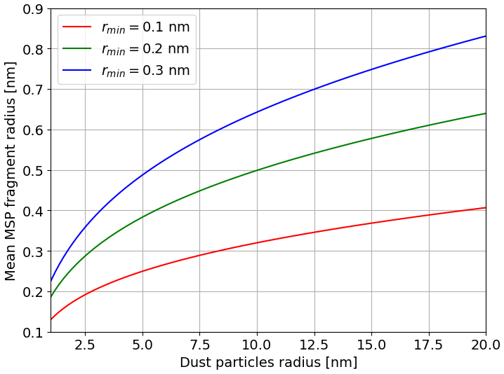
Figure A1 Mean MSP fragment radius as a function of the dust particle radius for three different value of r_min.

Appendix B: Airflows around the instrument for different altitudes and rocket speeds

Figures B1–B4 show the densities and the streams of the background gas around the detector for 80, 82, 85 and 90 km, respectively, and for the three different rocket speeds in each case. The airflow is very similar. For all cases, a bow shock is created on top of the funnel, leading to an increase in the air density, which becomes even more important in the instrument where it is the highest. These two increases in density will lead to a stronger drag force slowing down the mesospheric dust particles. Increasing the rocket speed leads to higher densities and stronger bow shocks, while a higher altitude leads to smaller densities and a weaker bow shocks.

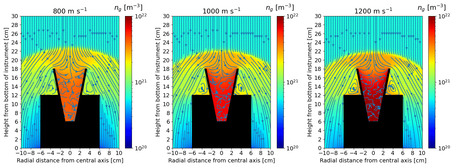
Figure B1 DSMC results for 80 km showing the background gas density n_g and stream around the detector for 800, 1000 and 1200 m s⁻¹ rocket speeds.

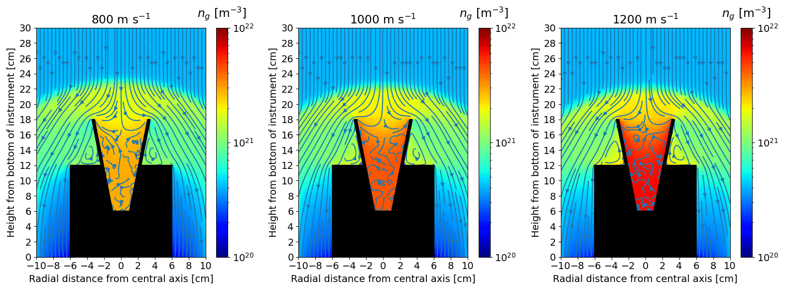
Figure B2 DSMC results for 82 km showing the background gas density n_g and stream around the detector for 800, 1000 and 1200 m s⁻¹ rocket speeds.

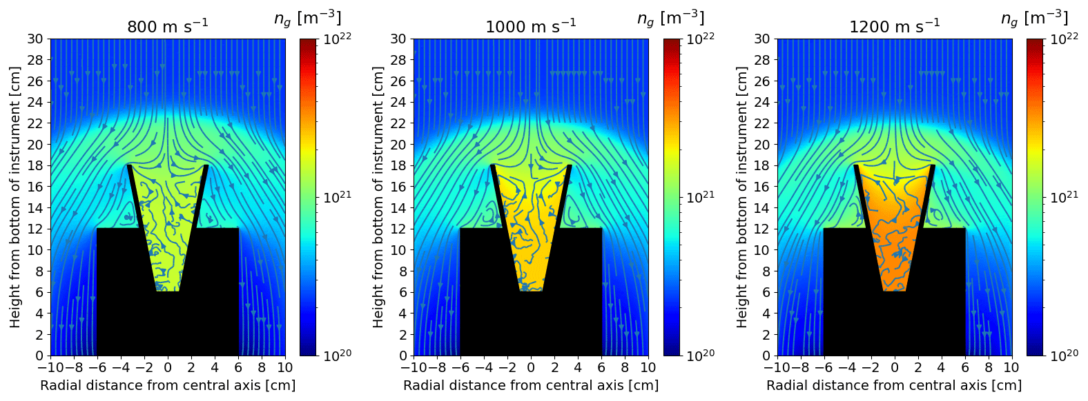
Figure B3 DSMC results for 85 km showing the background gas density n_g and stream around the detector for 800, 1000 and 1200 m s⁻¹ rocket speeds.

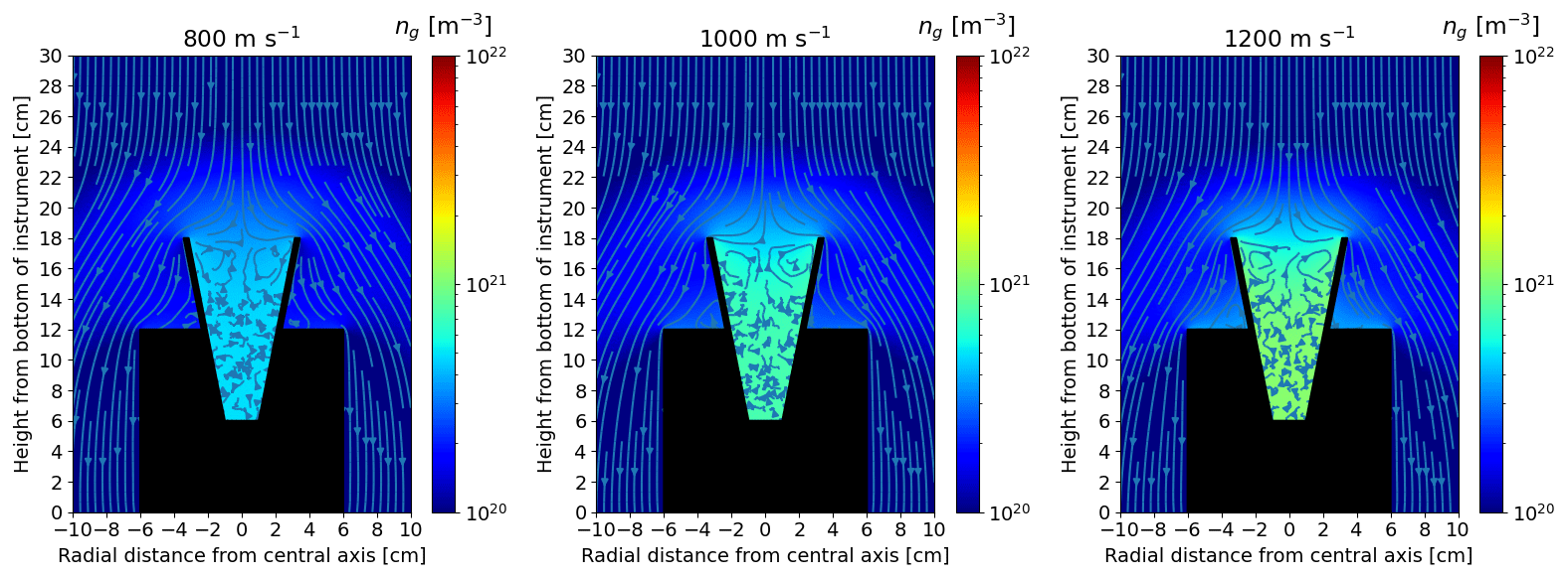
Figure B4 DSMC results for 90 km showing the background gas density n_g and stream around the detector for 800, 1000 and 1200 m s⁻¹ rocket speeds.