Lidar–radar synergistic method to retrieve ice, supercooled water and mixed-phase cloud properties

Mixed-phase clouds are not well represented in climate and weather forecasting models, due to a lack of the key processes controlling their life cycle. Developing methods to study these clouds is therefore essential, despite the complexity of mixed-phase cloud processes and the difficulty of observing two cloud phases simultaneously. We propose in this paper a new method to retrieve the microphysical properties of mixed-phase clouds, ice clouds and supercooled water clouds using airborne or satellite radar and lidar measurements, called VarPy-mix. This new approach extends an existing variational method developed for ice cloud retrieval using lidar, radar and passive radiometers. We assume that the lidar attenuated backscatter β at 532 nm is more sensitive to particle concentration and is consequently mainly sensitive to the presence of supercooled water. In addition, radar reflectivity Z at 95 GHz is sensitive to the size of hydrometeors and hence more sensitive to the presence of ice particles. Consequently, in the mixed phase the supercooled droplets are retrieved with the lidar signal and the ice particles with the radar signal, meaning that the retrievals rely strongly on a priori and error values. This method retrieves simultaneously the visible extinction for ice α_ice and liquid α_liq particles, the ice and liquid water contents IWC and LWC, the effective radius of ice r_e,ice and liquid r_e,liq particles, and the ice and liquid number concentrations N_ice and N_liq. Moreover, total extinction α_tot, total water content (TWC) and total number concentration N_tot can also be estimated. As the retrieval of ice and liquid is different, it is necessary to correctly identify each phase of the cloud. To this end, a cloud-phase classification is used as input to the algorithm and has been adapted for mixed-phase retrieval. The data used in this study are from DARDAR-MASK v2.23 products, based on the Cloud-Aerosol Lidar with Orthogonal Polarization (CALIOP) and Cloud Profiling Radar (CPR) observations from the CALIPSO and CloudSat satellites, respectively, belonging to the A-Train constellation launched in 2006. Airborne in situ measurements performed on 7 April 2007 during the Arctic Study of Tropospheric Aerosol, Clouds and Radiation (ASTAR) campaign and collected under the track of CloudSat–CALIPSO are compared with the retrievals of the new algorithm to validate its performance. Visible extinctions, water contents, effective radii and number concentrations derived from in situ measurements and the retrievals showed similar trends and are globally in good agreement. The mean percent error between the retrievals and in situ measurements is 39 % for α_liq, 398 % for α_ice, 49 % for LWC and 75 % for IWC. It is also important to note that temporal and spatial collocations are not perfect, with a maximum spatial shift of 1.68 km and a maximum temporal shift of about 10 min between the two platforms. In addition, the sensitivity of remote sensing and that of in situ measurements is not the same, and in situ measurement uncertainties are between 25 % and 60 %.

1 Introduction

The current situation concerning climate change strongly impacts our society (IPCC, 2022), which leads to an interest in climate and weather forecasting. Clouds cover about 67 % of Earth's atmosphere (King et al., 2013) and play an important role in Earth's water cycle and its radiation budget (Stephens, 2005). However, climate and weather prediction models still have a lack of knowledge in some situations and scenarios where clouds, especially mixed-phase clouds, remain one of the main sources of uncertainty, due to the complexity of the related processes. Mixed-phase clouds occur at all latitudes, more significantly at middle and high latitudes (Choi et al., 2010; Shupe, 2011), and are a coexisting mixture of three phases of water: ice particles, supercooled droplets and water vapor at temperatures between −40 and 0 °C. This coexistence implies complex formation processes, such as primary ice nucleation (Meyers et al., 1992), secondary ice production (Field et al., 2017; Kanji et al., 2017) and ice deposition (Meyers et al., 1992), and growing processes, such as the Wegener–Bergeron–Findeisen process (Wegener, 1911; Bergeron, 1935; Findeisen, 1938), water vapor deposition (Song and Lamb, 1994), aggregation (Hobbs et al., 1974) and riming (Hallett and Mossop, 1974). Since liquid and ice particles influence shortwave and longwave radiation differently (Matus and L'Ecuyer, 2017), the proportions of liquid and ice particles significantly affect the radiative properties of mixed-phase clouds, altering the radiative balance of Earth's atmospheric system. Moreover, all these processes are difficult to represent in numerical models (Morrison et al., 2008, 2012), and mixed-phase clouds that are not well represented in models can introduce significant biases such as a misrepresentation of the cloudy state (Pithan et al., 2014). For that reason it is crucial to have information on mixed-phase cloud microphysics in order to reduce the uncertainties in climate and weather prediction.

The localization and lifetime of the mixed phase in a cloud differ according to the type of cloud and can make cloud observation challenging. The difference in water vapor saturation over ice and liquid makes the mixed phase condensationally unstable and only exists for a limited time (Korolev et al., 2017). One way of observing these clouds is to use active remote sensing instruments. They can be on board an aircraft or a satellite, allowing us to probe clouds on a large scale with vertical profiles seen from above. They are therefore useful in detecting the mixed-phase layer at cloud top, which is typically the case in Arctic boundary layer clouds (Gayet et al., 2009; Mioche et al., 2017). Each instrument has its own characteristics and a specific sensitivity that depends notably on the instrument's wavelength. On one hand, lidar measures the attenuated backscatter β [m⁻¹ sr⁻¹], which corresponds to the energy backscattered by the targets and is affected by the atmospheric transmission. At a wavelength between 355 and 1064 nm, lidar attenuated backscatter is more sensitive to the concentration of hydrometeors and can detect small cloud particles and aerosols. However, this signal can be attenuated or extinguished by a region with high particle concentration and cannot give information below this cloud layer. On the other hand, radar measures the reflectivity Z [mm⁶ m⁻³] typically at 35 or 95 GHz for cloud radars. At these wavelengths radar reflectivity is more sensitive to particle size, and the signal can penetrate thick clouds (Delanoë et al., 2013; Cazenave et al., 2019). Consequently, in mixed-phase clouds lidar is more sensitive to highly concentrated liquid droplets and gives a strong backscatter signal. On the other hand, radar reflectivity of liquid droplets is weaker than that of ice particles. As a result, the two instruments complement each other. These measurements can therefore be used in algorithms to retrieve microphysical cloud properties such as the visible extinction α, the ice and liquid water contents (IWC and LWC, respectively), and the total number concentration N_tot.

Lidar–radar synergistic methods were first proposed by Intrieri et al. (1993), Donovan and van Lammeren (2001), Tinel et al. (2005), and Mitrescu et al. (2005) to retrieve ice cloud properties where both instruments overlap. Algorithms such as Varcloud (Delanoë and Hogan, 2008) and 2C-ICE (Deng et al., 2010) were later developed to retrieve ice cloud properties all along the instruments' profiles using the Cloud Profiling Radar (CPR) on board CloudSat (Stephens et al., 2002), the Cloud-Aerosol Lidar with Orthogonal Polarization (CALIOP) on board CALIPSO (Winker et al., 2003) and also radiometric information for Varcloud. For the EarthCARE mission (Illingworth et al., 2015) the unified synergistic retrieval algorithm CAPTIVATE (Mason et al., 2022) uses the Atmospheric Lidar (ATLID), CPR and multi-spectral imager (MSI) data to retrieve cloud, precipitation and aerosol properties.

The variational method Varcloud, developed by Delanoë and Hogan (2008), aims to retrieve ice cloud properties using radar, lidar and radiometric data synergy. Since its initial development, this algorithm has been improved with new parameterization for ice cloud retrieval (Ceccaldi, 2014; Cazenave et al., 2019), allowing more flexibility. As a result, it can process data from different airborne or spaceborne instruments' platforms. In the mixed phase, the algorithm only retrieves ice properties with the radar signal. The algorithm's current version is called VarPy-ice in this paper and is described in detail in Cazenave (2019, pp. 107–113). Our method, VarPy-mix, aims to retrieve simultaneously ice, supercooled water and mixed-phase cloud properties with lidar and radar synergy, based on VarPy-ice to retrieve ice clouds. Each cloud phase is not processed in the same way. The ice clouds are retrieved with both instruments, while the mixed-phase retrieval is divided into two parts: the ice particles are retrieved with the radar signal and the supercooled water with the lidar signal. Besides this, supercooled water clouds are retrieved with the lidar signal only. Therefore, the retrieval relies strongly on a priori and error values. Additionally, this flexible algorithm can be applied on several lidar–radar platforms, airborne or spaceborne. As a starting point, these changes were developed with CloudSat and CALIPSO instruments' datasets. These data have large, robust and proven classification algorithmic statistics, as well as existing cases of collocation with in situ measurements.

In Sect. 2 we describe the general points of both versions of VarPy before going into the details of the new-version structure. In addition, the processed cloud phases are presented along with an adaptation of the cloud-phase classification dedicated to the mixed phase and supercooled water. Section 3 presents a case of mixed phase at the top of an ice cloud for which microphysical properties are retrieved using VarPy-mix and compared with in situ measurements. In Sect. 4 we conclude the paper and provide an outlook on future work.

2 Methodology

2.1 Variational method

2.1.1 Description of VarPy

The radar reflectivity Z [mm⁶ m⁻³] and the lidar attenuated backscatter β [m⁻¹ sr⁻¹] are linked to the cloud microphysical vertical structure. For example, the water content is strongly correlated with the reflectivity (Atlas, 1954), and the lidar backscatter is related to the cloud extinction α. We can relate this situation to an inverse problem given by

$$\begin{array}{}\text{(1)}& \mathit{Y}=f\left(\mathit{X}\right)+\mathit{ϵ}.\end{array}$$

The vector Y is the observation vector composed of the measured radar reflectivity Z_obs and the lidar attenuated backscatter β_obs. The vector X is composed of the quantities that describe the system, e.g., some cloud microphysical properties. The function f is the “forward function” (Rodgers, 2000, p. 14) and in our case represents the lidar and the radar forward models. These models and measurements are associated with specific uncertainties that can be presented by the error vector ϵ. According to the values of the vector X (hereafter called the “state vector”), the forward models predict reflectivity and backscatter values, noted Z_fwd and β_fwd, respectively. These forward-modeled values are afterwards compared with the measurements. The difference between Y and the predicted values is used to update the state vector via the Gauss–Newton method. New values of Z_fwd and β_fwd are computed with the forward models and lookup table (LUT, detailed in Sect. 2.1.2) until convergence occurs according to a χ² test. The solution is defined by the state vector at the last iteration when the solution converges. These values are used in combination with an LUT to retrieve the desired microphysical properties. Figure 1 summarizes the whole structure of the variational scheme.

Figure 1 The sequence of operations executed by the VarPy retrieval method.

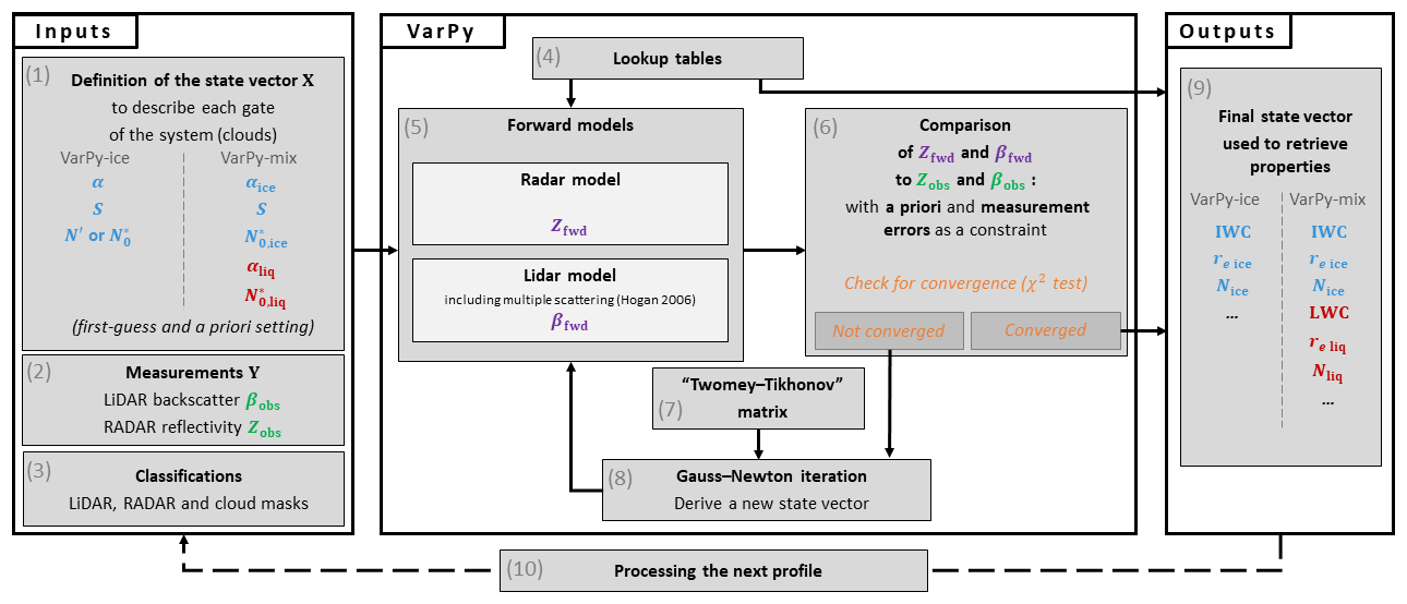
The two main inputs of VarPy are the observation vector Y (box 2 in Fig. 1; Eq. 2) and the initialized state vector X₀ (box 1 in Fig. 1), given by Eq. (5) with first-guess values from Table 1, as explained in Sect. 2.1.2. The natural logarithm is applied to the variables of X and Y to avoid the unphysical possibility of retrieving negative values. Both vectors are defined for one measurement profile and as a function of the distance from the instrument. Radar and lidar do not have the same number of values per profile (hereafter also called “gate”): there are q values of ln (Z_obs) for a profile and p values for ln (β_obs). Then the observation vector Y is defined for a single profile as follows:

$$\begin{array}{}\text{(2)}& \mathit{Y}=\left(\begin{array}{c}\ln \left(Z_{\mathrm{obs},\mathrm{0}}\right)\\ \mathrm{⋮}\\ \ln \left(Z_{\mathrm{obs},q}\right)\\ \\ \ln \left({\mathit{\beta }}_{\mathrm{obs},\mathrm{0}}\right)\\ \mathrm{⋮}\\ \ln \left({\mathit{\beta }}_{\mathrm{obs},p}\right)\end{array}\right).\end{array}$$

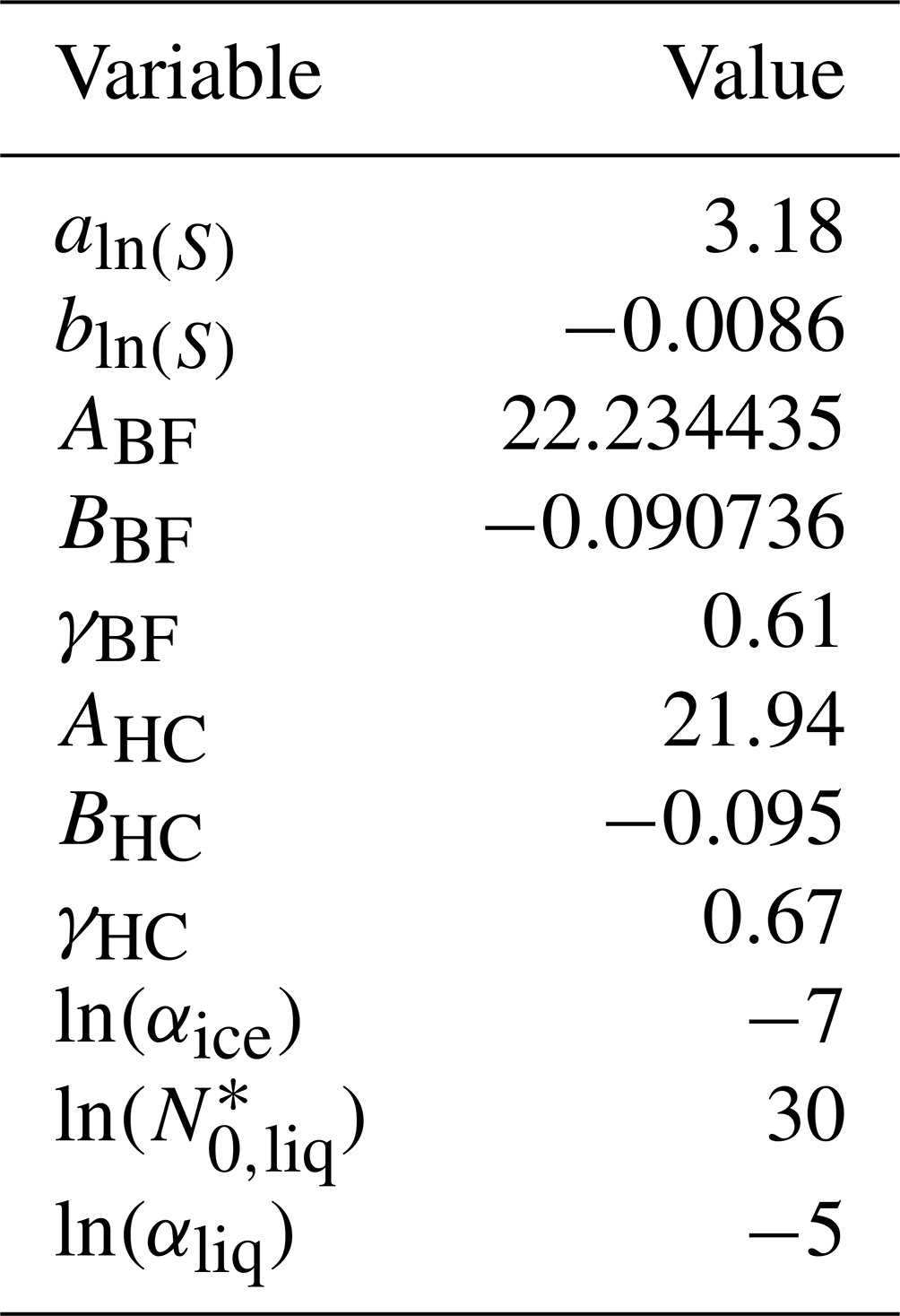
Table 1 The a priori and first-guess values for each variable of the state vector.

To retrieve ice properties, the state vector is composed of the visible extinction α [m⁻¹]; the extinction-to-backscatter ratio S [sr]; and N^′, which is related to the normalized number concentration parameter $N_{\mathrm{0}}^{\ast }$ [m⁻⁴] via the following relationship:

$$\begin{array}{}\text{(3)}& N^{\prime }={\displaystyle \frac{N_{\mathrm{0}}^{\ast }}{{\mathit{\alpha }}^{\mathit{\gamma }}}},\end{array}$$

where γ is an empirically determined coefficient normalizing N^′ (Delanoë and Hogan, 2010; Delanoë et al., 2014). Values for this coefficient are shown in Table 1. For n measurement gates, the state vector is composed of n values of ln (α). However, N^′ is not retrieved for each gate. A cubic-spline basis function interpolates the N^′ profile with a number concentration parameter spacing factor η_N set to 4 and decreases the number of N^′ values to m such that smooth variation in range is guaranteed (Hogan, 2007; Delanoë and Hogan, 2008). This improves computing efficiency by reducing calculation time.

The lidar ratio is assumed to be a function of temperature T [°C], adapted from Platt et al. (2002) and derived using lidar–radar data from previous versions of DARDAR (Cazenave et al., 2019). Consequently, the lidar ratio S is not represented in the state vector for each gate but by the two coefficients a_ln (S) and b_ln (S), which are the slope and the intercept coefficients from the temperature-dependent relationship (Eq. 4). As a result, for this configuration of the state vector, the dimension of the lidar ratio S is given by k=2. For VarPy-ice the average retrieved lidar ratio equals 35 ± 10 sr for a temperature range from −60 to −20 °C (Cazenave et al., 2019):

$$\begin{array}{}\text{(4)}& \ln \left(S\right)=a_{\ln \left(S\right)}+b_{\ln \left(S\right)}\cdot T.\end{array}$$

Thus, for VarPy-ice the state vector to retrieve a profile of n gates is as follows:

$$\begin{array}{}\text{(5)}& {\mathit{X}}_{\mathrm{ice}}=\left(\begin{array}{c}\ln \left(N_{\mathrm{0}}^{\prime }\right)\\ \mathrm{⋮}\\ \ln \left(N_m^{\prime }\right)\\ \\ a_{\ln \left(S\right)}\\ b_{\ln \left(S\right)}\\ \\ \ln \left({\mathit{\alpha }}_{\mathrm{0}}\right)\\ \mathrm{⋮}\\ \ln \left({\mathit{\alpha }}_n\right)\end{array}\right).\end{array}$$

The update of the state vector (box 8 in Fig. 1) is given by

$$\begin{array}{}\text{(6)}& \begin{array}{rl}{\mathit{X}}_{k+\mathrm{1}}& ={\mathit{X}}_k+{\mathbf{H}}^{-\mathrm{1}}\cdot \left({\mathbf{J}}^{\mathrm{T}}\cdot {\mathbf{R}}^{-\mathrm{1}}\cdot \left({\mathit{Y}}_{\mathrm{osb}}-{\mathit{Y}}_{\mathrm{fwd}}\right)\right.\\ & \left.-{\mathbf{B}}^{-\mathrm{1}}\cdot \left({\mathit{X}}_k-{\mathit{X}}_a\right)-\mathbf{T}\cdot {\mathit{X}}_k\right),\end{array}\end{array}$$

with J the Jacobian matrix that contains the partial derivative of ln (Z_fwd) and ln (β_fwd) with respect to each element of the state vector (box 5 in Fig. 1), H the Hessian matrix given by Eq. (7), R the error covariance matrix of the observations, B the error covariance matrix of the a priori values (explained in Sect. 2.2.1), and T the “Twomey–Tikhonov” matrix (box 7 in Fig. 1; Rodgers, 2000) used to smooth the extinction profile:

$$\begin{array}{}\text{(7)}& \mathbf{H}={\mathbf{J}}^{\mathrm{T}}\cdot {\mathbf{R}}^{-\mathrm{1}}\cdot \mathbf{J}+{\mathbf{B}}^{-\mathrm{1}}+\mathbf{T}.\end{array}$$

Each measurement is limited by the instrument's performance and the signal-to-noise ratio. This is notably the case for the lidar and can affect the retrieval of the extinction (Hogan et al., 2006). To limit the impact of measurement noise, a Twomey–Tikhonov matrix T can be used to penalize the second derivative of the state vector variables' profiles, especially the extinction. T is a square matrix and is defined at dimension 6 by

$$\begin{array}{}\text{(8)}& \mathbf{T}=\mathit{\kappa }\times \left(\begin{array}{rrrrrr}\mathrm{1}& -\mathrm{2}& \mathrm{1}& \mathrm{0}& \mathrm{0}& \mathrm{0}\\ -\mathrm{2}& \mathrm{5}& -\mathrm{4}& \mathrm{1}& \mathrm{0}& \mathrm{0}\\ \mathrm{1}& -\mathrm{4}& \mathrm{6}& -\mathrm{4}& \mathrm{1}& \mathrm{0}\\ \mathrm{0}& \mathrm{1}& -\mathrm{4}& \mathrm{6}& -\mathrm{4}& \mathrm{1}\\ \mathrm{0}& \mathrm{0}& \mathrm{1}& -\mathrm{4}& \mathrm{5}& -\mathrm{2}\\ \mathrm{0}& \mathrm{0}& \mathrm{0}& \mathrm{1}& -\mathrm{2}& \mathrm{1}\end{array}\right),\end{array}$$

where κ is a coefficient that sets the smoothness degree of T. The dimensions of the final matrix T used by the algorithm correspond to those of the state vector depending on the version of VarPy. As we only want to smooth the extinction profile, the values of T corresponding to the lidar ratio S and the number concentration parameter N^′ are set to 0.

The Jacobian matrix is a product of the forward models (box 5 in Fig. 1), and its composition depends on the structure of the state vector. For VarPy-ice this matrix is given by Eq. (9) with a dimension of $(p+q)\times (m+\mathrm{2}+n)$:

$$\begin{array}{}\text{(9)}& \mathbf{J}=\left(\begin{array}{cccccccc}\frac{\partial {\mathit{\beta }}_{\mathrm{0}}}{\partial N_{\mathrm{0}}^{\prime }}& \mathrm{\dots }& \frac{\partial {\mathit{\beta }}_{\mathrm{0}}}{\partial N_m^{\prime }}& \frac{\partial {\mathit{\beta }}_{\mathrm{0}}}{\partial a_{\ln \left(S\right)}}& \frac{\partial {\mathit{\beta }}_{\mathrm{0}}}{\partial b_{\ln \left(S\right)}}& \frac{\partial {\mathit{\beta }}_{\mathrm{0}}}{\partial {\mathit{\alpha }}_{\mathrm{0}}}& \mathrm{\dots }& \frac{\partial {\mathit{\beta }}_{\mathrm{0}}}{\partial {\mathit{\alpha }}_n}\\ \mathrm{⋮}& \mathrm{\ddots }& \mathrm{⋮}& \mathrm{⋮}& \mathrm{⋮}& \mathrm{⋮}& \mathrm{\ddots }& \mathrm{⋮}\\ \frac{\partial {\mathit{\beta }}_p}{\partial N_{\mathrm{0}}^{\prime }}& \mathrm{\dots }& \frac{\partial {\mathit{\beta }}_p}{\partial N_m^{\prime }}& \frac{\partial {\mathit{\beta }}_p}{\partial a_{\ln \left(S\right)}}& \frac{\partial {\mathit{\beta }}_p}{\partial b_{\ln \left(S\right)}}& \frac{\partial {\mathit{\beta }}_p}{\partial {\mathit{\alpha }}_{\mathrm{0}}}& \mathrm{\dots }& \frac{\partial {\mathit{\beta }}_p}{\partial {\mathit{\alpha }}_n}\\ \frac{\partial Z_{\mathrm{0}}}{\partial N_{\mathrm{0}}^{\prime }}& \mathrm{\dots }& \frac{\partial Z_{\mathrm{0}}}{\partial N_m^{\prime }}& \frac{\partial Z_{\mathrm{0}}}{\partial a_{\ln \left(S\right)}}& \frac{\partial Z_{\mathrm{0}}}{\partial b_{\ln \left(S\right)}}& \frac{\partial Z_{\mathrm{0}}}{\partial {\mathit{\alpha }}_{\mathrm{0}}}& \mathrm{\dots }& \frac{\partial Z_{\mathrm{0}}}{\partial {\mathit{\alpha }}_n}\\ \mathrm{⋮}& \mathrm{\ddots }& \mathrm{⋮}& \mathrm{⋮}& \mathrm{⋮}& \mathrm{⋮}& \mathrm{\ddots }& \mathrm{⋮}\\ \frac{\partial Z_q}{\partial N_{\mathrm{0}}^{\prime }}& \mathrm{\dots }& \frac{\partial Z_q}{\partial N_m^{\prime }}& \frac{\partial Z_q}{\partial a_{\ln \left(S\right)}}& \frac{\partial Z_q}{\partial b_{\ln \left(S\right)}}& \frac{\partial Z_q}{\partial {\mathit{\alpha }}_{\mathrm{0}}}& \mathrm{\dots }& \frac{\partial Z_q}{\partial {\mathit{\alpha }}_n}\end{array}\right).\end{array}$$

For better readability, the indices _fwd of Z and β are not displayed and the natural logarithms of Z, β, $N_{\mathrm{0}}^{\ast }$ and α are not written.

2.1.2 State vector parameterization

During the iterative process, the state vector variables are used by the forward models (radar and lidar) to compute the radar reflectivity Z_fwd and the lidar backscatter β_fwd. The lidar forward model differs from the radar forward model because an additional step is required to obtain β_fwd with the equivalent area radius r_a and the multiscatter code from Hogan (2006) (box 5 in Fig. 1). To obtain Z_fwd and r_a, the ratio $\frac{\mathit{\alpha }}{N_{\mathrm{0}}^{\ast }}$ derived from the state vector is linked to these variables via a one-dimensional LUT (box 4 in Fig. 1), which is also used to retrieve cloud microphysical properties (box 9 in Fig. 1) such as the effective radius r_e and the ice water content IWC. The ice cloud properties can be retrieved with two types of LUT. The “Heymsfield Composite” (HC) LUT uses the transition matrix (T-matrix) method and the mass–size relationship from Heymsfield et al. (2010). The “Brown and Francis modified” (BF) LUT is based on a combination of Brown and Francis (1995) and Mitchell (1996) mass–size relationships. These LUTs are used for DARDAR-CLOUD v3.00 and v3.10 products (Delanoë, 2023a, b), and more details about them can be found in Delanoë et al. (2014) and Cazenave (2019). For both VarPy-ice and VarPy-mix, both LUTs can be used to retrieve the ice properties, and one must be selected beforehand. Regarding the retrieval of the liquid part of the mixed-phase and supercooled water clouds, an LUT has been created and more details can be found in Sect. 2.2.2.

The LUT setting also involves defining the a priori and first-guess values of the state vector. The first-guess values are used to initialize the state vector for the forward models before the first iteration, corresponding to X₀. The a priori values are important for regions where only one instrument is available, and this constrains the scheme towards temperature-dependent empirical relationships. We have postulated in Sect. 2.1.1 that the lidar ratio is given by a temperature-dependent relationship (Eq. 4), and a priori and first-guess values are listed in Table 1. For the number concentration parameter ln (N^′), the a priori and first-guess values are also given as a function of the temperature T:

$$\begin{array}{}\text{(10)}& \ln \left(N^{\prime }\right)=(A+B\cdot T).\end{array}$$

Table 1 lists the values of A and B used for each mass–size relationship (BF and HC). The coefficient γ linking $N_{\mathrm{0}}^{\ast }$ to α and N^′ differs according to the mass–size relationship, and the values are also given in Table 1. The a priori and first-guess values for the extinction are constant values.

2.1.3 Definition of VarPy versions

Before going into the details of the adaptations made in VarPy-mix to retrieve supercooled water and mixed-phase clouds, we describe in this section the main assumptions about the instruments used for VarPy-ice and VarPy-mix.

VarPy-ice retrieves ice properties from radar and lidar measurements, including ice from mixed-phase layers. Since the lidar signal is more sensitive to liquid droplets than ice particles, it cannot be used in VarPy-ice to retrieve ice properties of mixed phase. Therefore, every lidar gate below the mixed-phase layer cannot be used due to the attenuation of the liquid droplets in the lidar signal. Consequently, the mixed phase and the ice cloud below are not retrieved via lidar–radar synergy but only with the radar signal and the state vector a priori values.

The main hypothesis for the VarPy-mix version is to consider the ice and liquid parts of the mixed phase separately and retrieve the liquid part with the lidar signal and the ice part with the radar signal. This hypothesis is based on the sensitivity of the instruments as explained in Sect. 1. The aim of this version of the algorithm is to be able to retrieve several cloud phases using the same variational method but with a structure and parameterization that are adapted to supercooled water and the mixed phase. A large part of VarPy-ice has been preserved to maintain the strengths of the method and the consistency of the results.

2.2 New configuration of the state vector to retrieve ice and supercooled water simultaneously

For the new version of the algorithm, the state vector needs to be adapted to also retrieve supercooled water properties. The special case of the mixed phase has to be taken into account. The supercooled water and the ice particle properties are retrieved separately for the mixed phase. The state vector is consequently divided into two parts: one part of the variables retrieves ice properties, and the other part retrieves liquid properties. The ice particles of the mixed phase are included in the ice part, and the supercooled droplets are in the liquid part. The composition of the state vector differs from the previous version and will be described in the following paragraphs.

As the liquid droplet concentration does not depend on the air temperature like for ice particles, the temperature-dependent concentration parameter N^′ is not required to retrieve liquid cloud properties. For this, we decided to use $N_{\mathrm{0}}^{\ast }$ in the state vector, instead of N^′. It can be noted that the VarPy-ice algorithm also has the ability to retrieve ice properties using the normalized number concentration parameter $N_{\mathrm{0}}^{\ast }$. This enables the VarPy-mix retrieval to be compared with the VarPy-ice retrieval to avoid any inconsistencies. We include this variable for each state vector part, so there is $N_{\mathrm{0},\mathrm{ice}}^{\ast }$ for the ice part and $N_{\mathrm{0},\mathrm{liq}}^{\ast }$ for the liquid part. Choosing $N_{\mathrm{0}}^{\ast }$ allows us to keep the a priori and first-guess values for the ice with the following temperature-dependent relationship:

$$\begin{array}{}\text{(11)}& \ln \left(N_{\mathrm{0},\mathrm{ice}}^{\ast }\right)=(A+B\cdot T)+\mathit{\gamma }\cdot \ln {\mathit{\alpha }}_{\mathrm{ice}}.\end{array}$$

This relation is based on Eq. (10) to calculate N^′ a priori and first-guess values. To keep the old scheme benefits, the cubic-spline basis function interpolates the $N_{\mathrm{0},\mathrm{ice}}^{\ast }$ values with a spacing factor η_N set to 4. It is unusable for the liquid group since supercooled layers are thin and correspond to too few gates.

Pinnick et al. (1983)O'Connor et al. (2004)Hogan et al. (2003)

Table 2 Lidar ratio S for liquid droplets depending on cloud type, particle size and lidar wavelength.

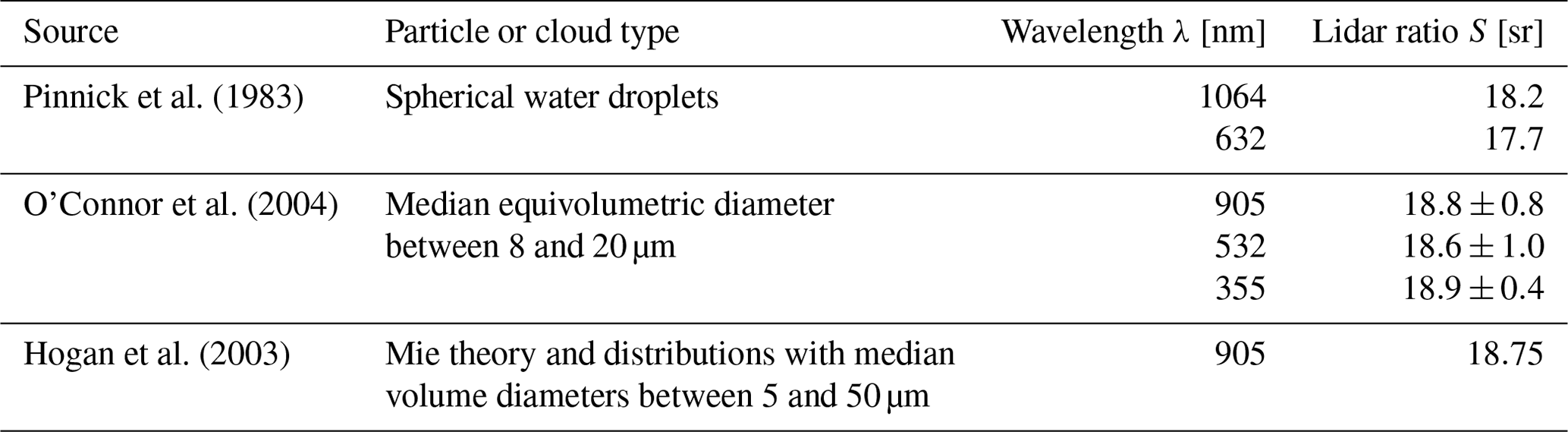
The extinction α is still part of the state vector. Like for $N_{\mathrm{0},\mathrm{ice}}^{\ast }$ and $N_{\mathrm{0},\mathrm{liq}}^{\ast }$, the extinction is divided into two variables: α_ice for the ice properties and α_liq for the liquid ones. Both variables are defined for each gate of a profile. Regarding the lidar ratio S, we keep the same configuration in the state vector with the two coefficients a_ln (S) and b_ln (S). Table 2 lists the values of the lidar ratio at different wavelengths and according to particle size or type. As a result, we make the assumption that the lidar ratio is constant for liquid droplets (Pinnick et al., 1983). Consequently, the lidar ratio is defined only for ice gates in the state vector, and its value is fixed at 18.6 sr for supercooled water (pure or in mixed phase) at 532 nm.

For the number of ice gates n_i, the number of liquid gates n_l and m_i defined in the same way as m depending on the spacing parameter η_N, we end up with the new state vector given by Eq. (12):

$$\begin{array}{}\text{(12)}& {\mathit{X}}_{\mathrm{mix}}=\left(\begin{array}{c}\ln \left(N_{\mathrm{0},\mathrm{ice},\mathrm{0}}^{\ast }\right)\\ \mathrm{⋮}\\ \ln \left(N_{\mathrm{0},\mathrm{ice},m_i}^{\ast }\right)\\ a_{\ln \left(S\right)}\\ b_{\ln \left(S\right)}\\ \ln \left({\mathit{\alpha }}_{\mathrm{ice},\mathrm{0}}\right)\\ \mathrm{⋮}\\ \ln \left({\mathit{\alpha }}_{\mathrm{ice},n_i}\right)\\ \\ \ln \left(N_{\mathrm{0},\mathrm{liq},\mathrm{0}}^{\ast }\right)\\ \mathrm{⋮}\\ \ln \left(N_{\mathrm{0},\mathrm{liq},n_l}^{\ast }\right)\\ \ln \left({\mathit{\alpha }}_{\mathrm{liq},\mathrm{0}}\right)\\ \mathrm{⋮}\\ \ln \left({\mathit{\alpha }}_{\mathrm{liq},n_l}\right)\end{array}\right).\end{array}$$

For VarPy-ice, a single Twomey–Tikhonov matrix of the dimensions ($m+k+n$) × ($m+k+n$) is applied for the entire extinction profile. However, the extinction values of liquid droplets are different from ice particles, and it is therefore unsuitable to use a single Twomey–Tikhonov matrix on a profile with simultaneously ice and supercooled water. As we want to smooth the extinction profile for both ice and liquid parts, we decided to smooth them out separately and not to use a single Twomey–Tikhonov matrix to smooth out an entire profile. Consequently, for VarPy-mix a method has been developed to separate different sections of a profile according to the smoothing to be applied. The separation is made between ice, liquid and where there is clear sky. Then one Twomey–Tikhonov matrix is applied to each section. The dimensions of the final matrix are ($m_i+k+n_i+\mathrm{2}\times n_l$) × ($m_i+k+n_i+\mathrm{2}\times n_l$). The smoothness coefficient κ is set to 100 for VarPy-ice, and this parameterization is kept for the ice part of VarPy-mix, whereas the coefficient applied to the liquid water is different and set to 10 since the thickness of the detected liquid layer is smaller than that of the ice layer.

2.2.1 The a priori error covariance matrix

Generally, radar and lidar signals do not both cover the entire vertical cloud profile simultaneously. In many cases of ice clouds, lidar in the downward direction first detects the top of the cloud, while radar only detects deeper cloud regions down to the ground. The lidar signal will not detect the lower layers of the cloud if it gets attenuated or extinguished. To ensure that the results tend towards physical values in regions where a single instrument is available, state vector a priori parameterization and errors are used. The a priori errors are defined by the a priori error covariance matrix B and express the strength level of the constraint of the a priori errors. This matrix is composed of the error variances of the state vector a priori σ². In the simplest case where no information propagates between gates, this matrix is diagonal.

To overcome the limitation of single-instrument retrieval, the matrix B can be used to spread information in height. Additional off-diagonal elements can be added to propagate information from synergistic regions to single-instrument ones. In VarPy-ice (Hogan, 2007; Delanoë and Hogan, 2008) the off-diagonal terms of B corresponding to N^′ are given by​​​​​​​

$$\begin{array}{}\text{(13)}& B_{i,j}=B_{i,i}\times e^{-\frac{|z_j-z_i|}{z_{\mathrm{0}}}},\end{array}$$

where z₀ is the decorrelation distance, a parameter set to 600 m for VarPy (initially set to 1 km for Varcloud). This value is set for CloudSat–CALIPSO and can be adapted to the resolution of the data used.

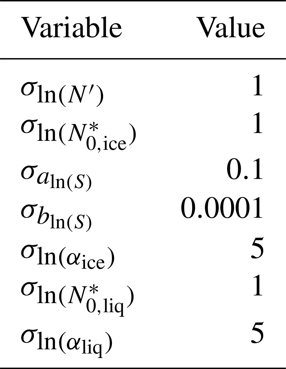
In the VarPy-mix version the structure of B has been adapted to the composition of the new state vector. In order to keep the same configuration as VarPy-ice, the off-diagonal terms are calculated for $N_{\mathrm{0},\mathrm{ice}}^{\ast }$ only. As a result, B remains diagonal regarding the other variables. The a priori error variance values for both VarPy-ice and VarPy-mix are listed in Table 3 and are assumed to be constant with height.

Table 3 The a priori error variances used in VarPy for the a priori error covariance matrix B.

In addition, the dimensions of the matrices U and M, used for the calculation of the error covariance matrix of the state vector S_x (refer to Appendix A of Delanoë and Hogan, 2008, for more information), have been adapted to the number of variables in X_mix and their dimensions.

2.2.2 Normalized droplet size distribution for liquid lookup table

For VarPy-ice and VarPy-mix, ice properties are retrieved using dedicated LUTs, which are created using the particle size distribution of ice particles (Delanoë et al., 2014). However, the particle size distribution differs between ice particles and liquid droplets, meaning that LUTs dedicated to the retrieval of ice properties cannot be used to retrieve liquid properties. The solution is to define a droplet size distribution (DSD) for liquid droplets to create an LUT dedicated to the retrieval of liquid properties. Regarding the literature, there are two types of distribution: the gamma distribution (Miles et al., 2000) and the log-normal distribution (Frisch et al., 1995; Fielding et al., 2015). For this study we use the following log-normal relationship defined by Frisch et al. (1995):

$$\begin{array}{}\text{(14)}& n\left(r\right)={\displaystyle \frac{N_{\mathrm{liq}}}{\mathit{\sigma }\sqrt{\mathrm{2}\mathit{\pi }}}}{e}^{-\frac{{\left(\ln \left(r\right)-\ln \left(r_{\mathrm{0}}\right)\right)}^{\mathrm{2}}}{\mathrm{2}{\mathit{\sigma }}^{\mathrm{2}}}},\end{array}$$

where n(r) is the number concentration at a given cloud droplet radius r [µm], N_liq is the total number of liquid droplets per unit volume [m⁻³], r₀ is the modal radius [µm] and σ is the geometric standard deviation. The kth moment 〈r^k〉 of this distribution can be expressed as follows:

$$\begin{array}{}\text{(15)}& \langle r^k\rangle ={\displaystyle \frac{\mathrm{1}}{N_{\mathrm{liq}}}}\underset{\mathrm{0}}{\overset{\mathrm{\infty }}{\int }}n\left(r\right)r^k\mathrm{d}r.\end{array}$$

It permits us to relate the following variables to D_m [m] (proportionally to the ratio between the fourth moment and the third moment):

• the reflectivity Z [mm⁶ m⁻³], which is proportional to the sixth moment of the DSD;

• the extinction α [m⁻¹], which is proportional to the second moment;

• the liquid water content LWC [kg m⁻³], which is proportional to the third moment;

• the effective radius r_e [m], which is proportional to the ratio between the third moment and the second moment;

• the equivalent area radius r_a [m], which is equivalent to r_e for droplets;

• the total number of liquid droplets per unit volume N_liq [m⁻³].

Those quantities are then normalized by $N_{\mathrm{0}}^{\ast }$ [m⁻⁴], which can also be expressed as a function of D_m using the moments of the distribution (proportionally to the ratio between the third moment to the fifth power and the fourth moment to the fourth power). The LUT ends up being composed of $\frac{Z}{N_{\mathrm{0}}^{\ast }}$,$\frac{\mathit{\alpha }}{N_{\mathrm{0}}^{\ast }}$, $\frac{LWC}{N_{\mathrm{0}}^{\ast }}$, $\frac{N_{\mathrm{liq}}}{N_{\mathrm{0}}^{\ast }}$, r_a and r_e as a function of D_m. As with ice LUT, the liquid one is used in two steps of the algorithm with the ratio $\frac{\ln \left({\mathit{\alpha }}_{\mathrm{liq}}\right)}{\ln \left(N_{\mathrm{0},\mathrm{liq}}^{\ast }\right)}$ from the state vector values. This ratio is used to retrieve the corresponding value in LUT, by interpolation, first, at each iteration, to predict ln Z_fwd, ln β_fwd (via ln r_a and the fast multiple-scattering model of Hogan, 2006) and the Jacobian terms with the forward models. Then, with the final state vector, the ratio $\frac{\ln \left({\mathit{\alpha }}_{\mathrm{liq}}\right)}{\ln \left(N_{\mathrm{0},\mathrm{liq}}^{\ast }\right)}$ permits us to obtain LWC, r_e,liq and N_liq (box 9 in Fig. 1).

As explained in Sect. 2.1.1, two LUTs are available to retrieve ice properties. They are both implemented in VarPy-mix to retrieve the ice part of the mixed phase. Furthermore, they are defined in terms of the mean volume-weighted melted-equivalent diameter, which makes them very similar to the liquid LUT for small radii. This ensures scientific consistency and algorithm flexibility.

2.2.3 Jacobians

The Jacobian depends on the state vector composition and is different between VarPy-ice and VarPy-mix. The structure of the Jacobian J for VarPy-mix is shown by Eq. (16).​​​​​​​

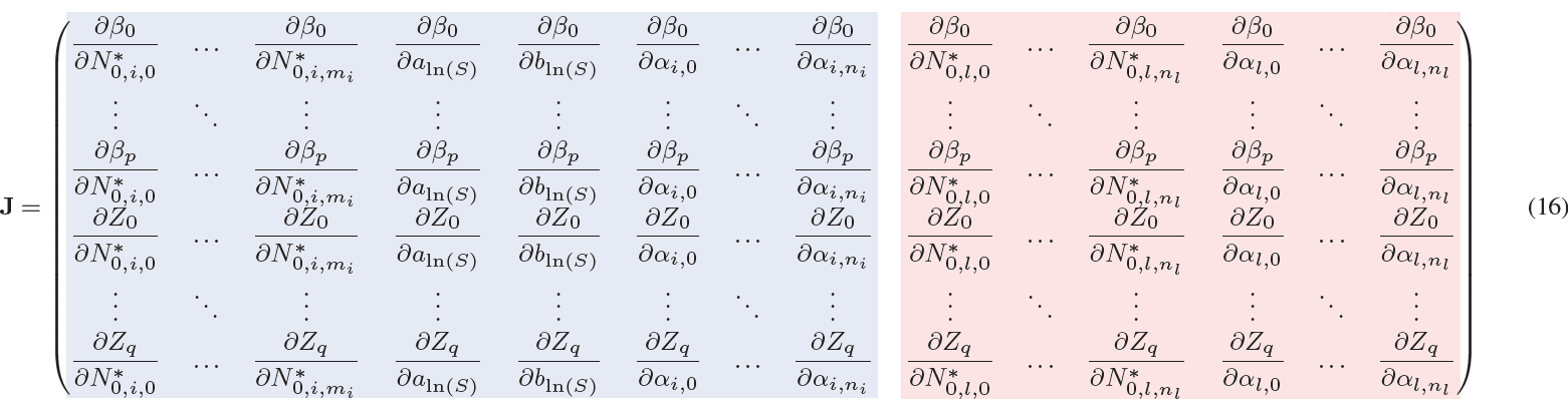
For better readability the indices _fwd of Z and β are not displayed; the _ice and _liq indices of $N_{\mathrm{0}}^{\ast }$ and α are replaced by the _i and _l indices, respectively; and the natural logarithms of Z, β, $N_{\mathrm{0}}^{\ast }$ and α are omitted. As with the state vector, we can divide the Jacobian into two parts: the derivatives of ln Z and ln β with respect to $\ln N_{\mathrm{0},\mathrm{ice}}^{\ast }$, a_ln (S), b_ln (S) and ln α_ice for the ice part (blue background color in Eq. 16) and the derivatives of ln Z and ln β with respect to $\ln N_{\mathrm{0},\mathrm{liq}}^{\ast }$ and ln α_liq for the liquid part (red background color). For the mixed phase both liquid and ice parts are used. However, each part is retrieved with only one instrument. Indeed, the radar is not used to retrieve the supercooled water either in pure liquid clouds or in mixed-phase clouds; therefore, $\frac{\partial \ln \left(Z_j\right)}{\partial \ln \left(N_{\mathrm{0},\mathrm{liq},k}^{\ast }\right)}$ and $\frac{\partial \ln \left(Z_j\right)}{\partial \ln \left({\mathit{\alpha }}_{\mathrm{liq},k}\right)}$ are zero for any values of j and k. The lidar is used to retrieve ice cloud properties but not the ice part of the mixed phase. Then, $\frac{\partial \ln \left({\mathit{\beta }}_j\right)}{\partial \ln \left(N_{\mathrm{0},\mathrm{ice},k}^{\ast }\right)}$ and $\frac{\partial \ln \left({\mathit{\beta }}_j\right)}{\partial \ln \left({\mathit{\alpha }}_{\mathrm{ice},k}\right)}$ are zero for any values of j and k corresponding to mixed-phase gates.

2.3 Cloud-phase classification

Ice particles and liquid droplets are processed differently, meaning that hydrometeor identification is an important algorithm input and more significantly regarding the mixed phase. The retrieval of cloud properties requires us to distinguish the different hydrometeors detected by the instruments – here the radar and the lidar. Therefore, according to the sensitivity of each instrument, a hydrometeor classification is established for each instrument. Lidar classification distinguishes aerosols and cloud phases, while radar classification identifies precipitation and clouds. Thus, combining the lidar and radar classifications results in a more detailed cloud-phase classification. These three classifications are additional inputs to the algorithm (box 3 in Fig. 1).

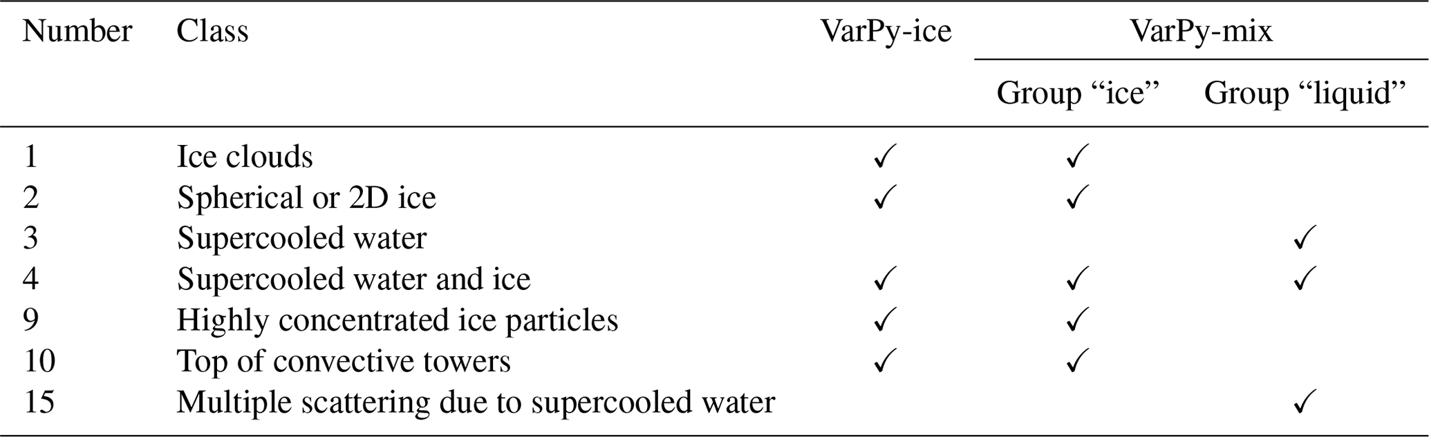
DARDAR-MASK v2.23 (Delanoë and Hogan, 2010) is a target categorization made by the combination of the 2B-GEOPROF CloudSat radar mask, the CALIPSO vertical lidar feature mask CAL-LID-L2-VFM and CALIPSO L1 measurements with a multi-threshold decision tree (Ceccaldi et al., 2013; Cazenave et al., 2019). VarPy algorithms use it in order to select the gates to process and how to process them. Table 4 shows the 18 classes of the DARDAR-MASK v2.23 classification. The classes are not all processed. Currently, the algorithm processes the “ice clouds”, the “spherical or 2D ice”, the “supercooled water”, the “supercooled water and ice”, the “highly concentrated ice particles”, the “top of convective towers”, and the “multiple scattering due to supercooled water” classes (highlighted in bold in Table 4). For VarPy-ice these classes form a single group to process. On the other hand, two groups of classes have been defined for VarPy-mix. Table 5 presents the composition of these groups. The group “ice” is composed of the following classes: “ice clouds”, “spherical or 2D ice”, “supercooled water and ice”, “highly concentrated ice particles”, and “top of convective towers”. The “supercooled water”, “supercooled water and ice” and “multiple scattering due to supercooled water” classes define the “liquid” group. This distinction is necessary to process the different phases of the clouds separately. Nevertheless, the “supercooled water and ice” class (called hereafter “mixed phase”) has the particularity of being processed in both the ice and the liquid groups. In the current versions of VarPy an intermediate classification, called the processed cloud-phase classification, is created with these groups. For the case used for this paper, the processed cloud-phase classification is presented in Fig. 2c.

Table 4 DARDAR-MASK v2.23 classes. The phases currently processed in VarPy-mix are those indicated in bold.

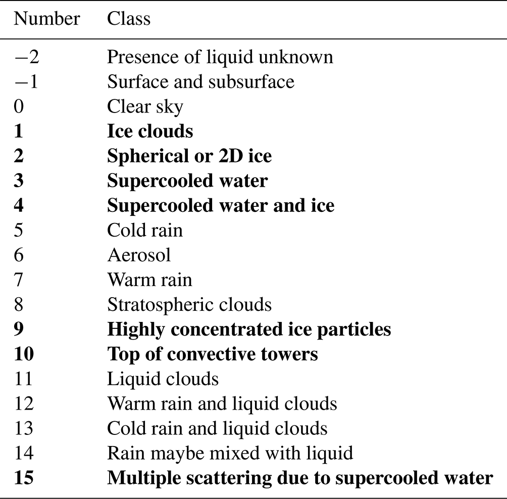
Table 5 Cloud phases processed by VarPy-ice and VarPy-mix. Single group for VarPy-ice and two groups (ice and liquid) for VarPy-mix.

Supercooled water layers are detected and identified using the lidar signal. In order to distinguish between the classes “supercooled water” and “supercooled water and ice”, the radar signal is used. On one hand, if the radar detects ice, the cloud-phase classification identifies the area as “supercooled water and ice”. On the other hand, where the radar does not detect particles (no radar signal) and the lidar backscatter is strong, it is categorized as “supercooled water” and the following gates are usually “multiple scattering due to supercooled water”. For these gates, retrievals are based only on lidar measurements and a priori values.

To minimize misclassification, some adaptations of the cloud-phase classification have been implemented. The first step is to avoid isolated gates that bias the retrieval. A method has been created to erode isolated supercooled water and mixed-phase gates. For supercooled water and multiple-scattering phases, these gates are replaced by clear sky in the cloud-phase classification and the same correction is made for the lidar classification. On the other hand, for the mixed phase only the cloud-phase classification is modified, and the gates are replaced by ice gates. Afterwards, the next step is to correct some misclassification of the mixed phase. A strong lidar backscatter signal (${\mathit{\beta }}_{\mathrm{532}}>{\mathrm{2.10}}^{-\mathrm{5}}$ m⁻¹ sr⁻¹; Delanoë and Hogan, 2010) can be a detection of warm water, the top of convective towers, highly concentrated ice particles or supercooled water. For CALIOP, DARDAR-MASK uses a decision tree to classify the mixed phase and differentiates it from highly concentrated ice particles for a temperature range from −40 to 0 °C (Ceccaldi et al., 2013). In some cases highly concentrated ice particle areas are incorrectly classified as mixed phase and need to be corrected for VarPy. These gates are then replaced by highly concentrated ice particles in the cloud-phase classification.

2.4 Summary of the methodology

In the previous subsections we described the principle and structure of the VarPy-mix method. Here we summarize the five main points of the method:

1. The radar reflectivity and the lidar backscatter measurements are the algorithm inputs. Their combination provides a cloud-phase classification. This information is essential, as supercooled droplets and ice particles are not processed the same way in our approach. We improve, correct and extend the classification to supercooled water (either pure or in the mixed phase).

2. The state vector is composed of variables linked to both the measurements and the microphysical properties to be retrieved. We propose a state vector structure that allows us to simultaneously retrieve both ice particle and supercooled water droplet properties (either pure or in the mixed phase).

3. We assume that the lidar ratio of liquid water is constant with a value of 18.6 sr.

4. Based on radar and lidar sensitivity, the ice part of the mixed phase is retrieved with the radar signal and the liquid part with the lidar signal. Consequently, this influences the Jacobian structure, which is calculated by the radar and lidar forward models.

5. The parameterization (errors, a priori values, first-guess values, LUT, smoothing parameters, etc.) to retrieve ice microphysical properties comes from VarPy-ice. For supercooled water properties a new parameterization is applied, and a new LUT is created based on a log-normal distribution.

3 Example of retrieval and comparison with collocated in situ measurements

During the Arctic Study of Tropospheric Aerosol, Clouds and Radiation (ASTAR; Gayet et al., 2009; Ehrlich et al., 2009) campaign, four legs coming from the same flight were performed on 7 April 2007 over the ocean near the Svalbard archipelago. The case presented in this study is one of the rare CloudSat–CALIPSO transects with collocated airborne in situ measurements of mixed-phase clouds. The in situ data from three probes are compared in this study to VarPy-mix retrievals. This comparison is possible because cloud detection and phase identification between DARDAR-MASK and in situ observations are in overall good agreement. Indeed, Mioche and Jourdan (2018) show that 91 % of clear-sky events and 86 % of the cloudy gates of DARDAR-MASK match the polar nephelometer in situ probe from samples collected during the ASTAR 2007 and POLARCAT 2008 (see the special issue on POLARCAT in Atmospheric Chemistry and Physics) campaigns. The polar nephelometer can also be used to estimate the cloud phase observed (ice, liquid water and mixed phase) thanks to thresholds on the asymmetry parameter g (Jourdan et al., 2010). Using the polar nephelometer as a reference, Mioche and Jourdan (2018) show that 61 % of DARDAR-MASK classification corresponding to the ice phase matches the polar nephelometer data, with 67 % for the liquid phase and 24 % for the mixed phase. This identification difference may be due to the temporal and spatial difference between satellite and in situ observations or to the detection limit of supercooled water by lidar due to attenuation.

3.1 Remote sensing and in situ measurements

For this comparison, the radar and lidar measurements, and the classifications, come from the DARDAR-MASK v2.23 product (Cazenave et al., 2019). The selected latitude range is shown in Fig. 2, which presents the profiles of the lidar backscatter measurements (Fig. 2a), the radar reflectivity (Fig. 2b), the processed cloud-phase classification (Fig. 2c) and the instrument flag to know which instrument is used for the retrieval (Fig. 2d). The strong lidar backscatter signal at the top of the cloud means that there is a large quantity of small particles like supercooled water droplets. As the radar also detects particles in this part of the cloud, this means that there are also ice particles. The processed cloud-phase classification thus shows the presence of an ice cloud with a mixed-phase layer at the top. As presented in Fig. 2d, the mixed phase is retrieved with both radar and lidar, and the ice cloud below is mainly retrieved with radar only, as the lidar is strongly attenuated and extinguished due to the supercooled water of the mixed phase. As a result, the base of the supercooled liquid layer within the mixed-phased cloud cannot be determined unequivocally.

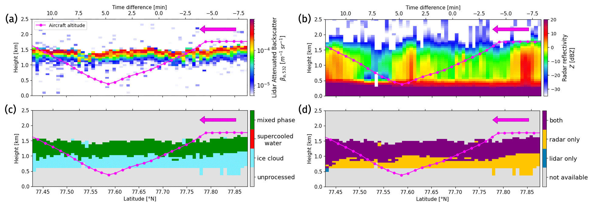
Figure 2 Selected profiles of CALIPSO attenuated backscatter (a), CloudSat reflectivity (b), processed cloud-phase classification (c) and instrument synergy (d). The trajectory and direction of Polar 2 are shown by the magenta line and arrow, respectively.

The three in situ instruments on board the Polar 2 aircraft were a cloud particle imager (CPI; Lawson et al., 1998), a forward-scattering spectrometer probe (FSSP-100; Dye and Baumgardner, 1984; Gayet et al., 2007) and a polar nephelometer (PN; Gayet et al., 1997). As the aircraft was not flying exactly along the satellites' trajectories, nor at the same time, the collocation is quite challenging. Among the four legs, the third one is temporarily the closest to the satellites' overpass with less than 10 min delay (shown on the top x axis in Fig. 2a and b). We focus this study on this leg to compare VarPy-mix retrievals to the in situ measurements. The altitude of the aircraft is shown by the magenta line in Fig. 2, where each point corresponds to a 30 s averaged probe measurement and the magenta arrow indicates the direction of the flight. As the aircraft flew above the cloud before going inside the cloud and passing through the mixed-phase layer twice, we have thus a vertical description of the cloud, and the comparison with VarPy-mix retrieval is more complete.

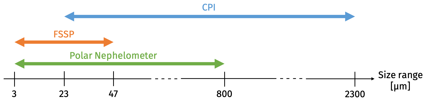
The size range sensitivity of each probe is presented in Fig. 3. We assume here that the CPI provides information on ice particles, while the FSSP provides information on liquid water. We cannot exclude the possibility that the FSSP also detects secondary ice particles (Costa et al., 2017) or could be more likely contaminated by ice crystals shattered on the instrument tips. However, Costa et al. (2017) showed that secondary ice particles are not frequent in Arctic mixed-phase clouds. The temperature range at which clouds were probed (between −21 and −14 °C) does not point towards possible secondary ice production mechanisms (above −10 °C). Additionally, Febvre et al. (2012) showed that when ice crystals are measured by the FSSP, the asymmetry parameter measured by the PN decreases compared with what would be expected for water droplets only. In our case study the asymmetry parameter g is mostly greater than 0.84 in the upper cloud layer, which is indicative of a layer composed quasi-exclusively of water droplets. Consequently, we are quite confident that the presence of small ice crystals does not significantly impact the results.

Figure 3 CPI, FSSP and PN range sensitivities.

For this study, we derive the ice cloud extinction α_CPI, the ice water content IWC_CPI, the ice effective radius r_e,CPI and the ice number concentration N_CPI from the CPI. The mass–size relationship to calculate IWC_CPI is given by Eq. (17) (model B for 0.2 kg m⁻² in Leinonen and Szyrmer, 2015). It corresponds to moderate riming and gives the best agreement over the whole flight:

$$\begin{array}{}\text{(17)}& m=\mathrm{0.033}\times D^{\mathrm{1.94}}.\end{array}$$

The liquid cloud extinction α_FSSP, liquid water content LWC_FSSP, liquid effective radius r_e,FSSP and liquid number concentration N_FSSP are provided by the FSSP. Both r_e,CPI and r_e,FSSP are calculated according to the following formula (Foot, 1988):

$$\begin{array}{}\text{(18)}& r_{\mathrm{e}}={\displaystyle \frac{\mathrm{3}}{\mathrm{2}}}{\displaystyle \frac{\mathrm{WC}}{\mathit{\rho }\mathit{\alpha }}},\end{array}$$

where r_e is the ice (r_e,CPI) or liquid (r_e,FSSP) effective radius, WC is the ice (IWC_CPI) or liquid (LWC_FSSP) water content, ρ is the density of ice (917 kg m⁻³) or water (1000 kg m⁻³), and α is the ice (α_CPI) or liquid (α_FSSP) extinction.

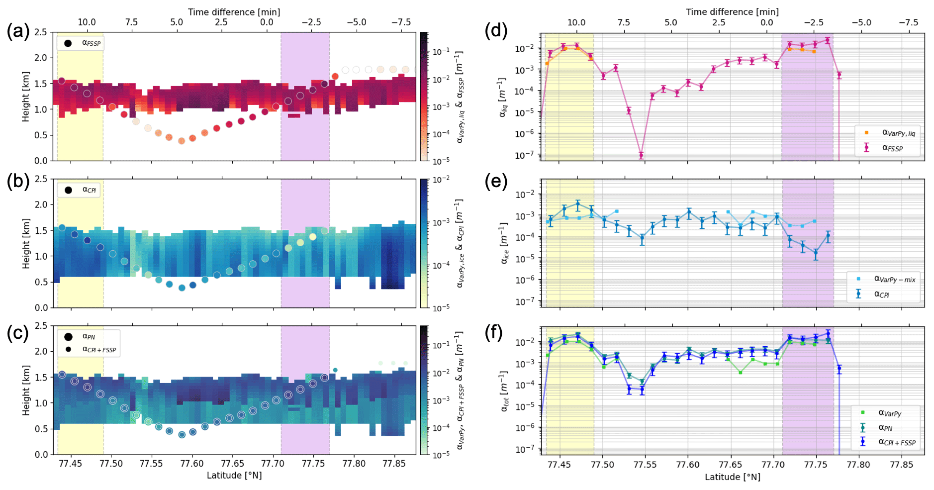
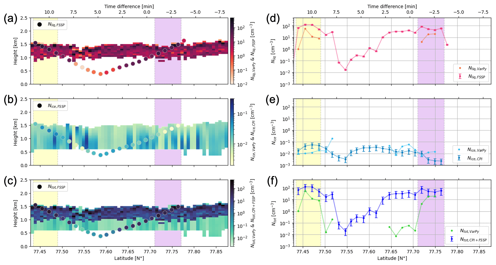
Figure 4 Panels (a)–(c) represent the liquid (a), ice (b) and total (c) extinctions from VarPy-mix retrievals (curtain) and in situ probes (dots) regarding the latitude and the height. Panels (d)–(f) represent the liquid (d), ice (e) and total (f) extinctions from VarPy-mix retrievals and in situ probes regarding the latitude. The error bars of in situ measurements (uncertainties from Table 6) are displayed in (d)–(f). The yellow and purple shading represents the latitude range where mixed-phase retrievals are compared with in situ measurements.

Figure 5 Same as Fig. 4 but for LWC, IWC and total water content (TWC).

Figure 6 Same as Fig. 4 but for r_e,liq and r_e,ice.

Figure 7 Same as Fig. 4 but for N_liq, N_ice and N_tot.

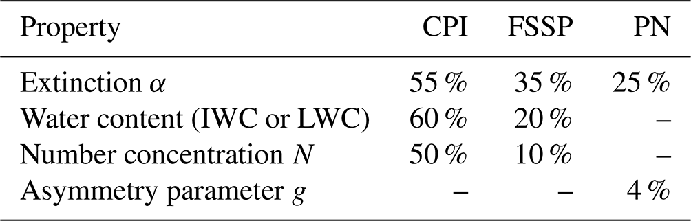
By summing extinctions, water contents and concentrations from both instruments, the total extinction α_CPI+FSSP, the total water content TWC_CPI+FSSP and the total number concentration N_CPI+FSSP can be obtained. In addition, the PN provides the total extinction α_PN. These in situ measurements are shown in Figs. 4–7 and are detailed in the comparison in Sect. 3.3. The uncertainties in extinctions, water contents, number concentrations and asymmetry parameters are presented in Table 6 (Mioche et al., 2017).

Table 6 Uncertainties in cloud properties derived from CPI, FSSP and PN probes from Mioche et al. (2017).

3.2 VarPy-mix retrievals

The cloud-phase classification has been adapted by eroding isolated supercooled gates. In this study we chose to retrieve ice properties with the HC LUT. This implies that the A_HC, B_HC and γ_HC values are used for the a priori and first-guess values of $\ln \left(N_{\mathrm{0},\mathrm{ice}}^{\ast }\right)$. For the liquid LUT, the only parameter of the size distribution that can vary is the geometric standard deviation σ. Fielding et al. (2014, 2015) set this value to σ=0.3 ± 0.1 and Frisch et al. (1995) to σ=0.35. We chose here to set the geometric standard deviation to σ=0.3.

First, the liquid and ice extinctions retrieved by VarPy-mix are shown by the curtain in Fig. 4a and b, respectively, and are used to access more liquid and ice properties via LUTs. Figure 5a and b show LWC and IWC, Fig. 6a and b show r_e,liq and r_e,ice, and Fig. 7a and b show N_liq and N_ice. For each microphysical property, the ice and liquid parts are retrieved according to the classification. For the ice cloud between 0.5 and 1 km, only the ice properties are available. Ice and liquid properties are both retrieved for the mixed-phase gates.

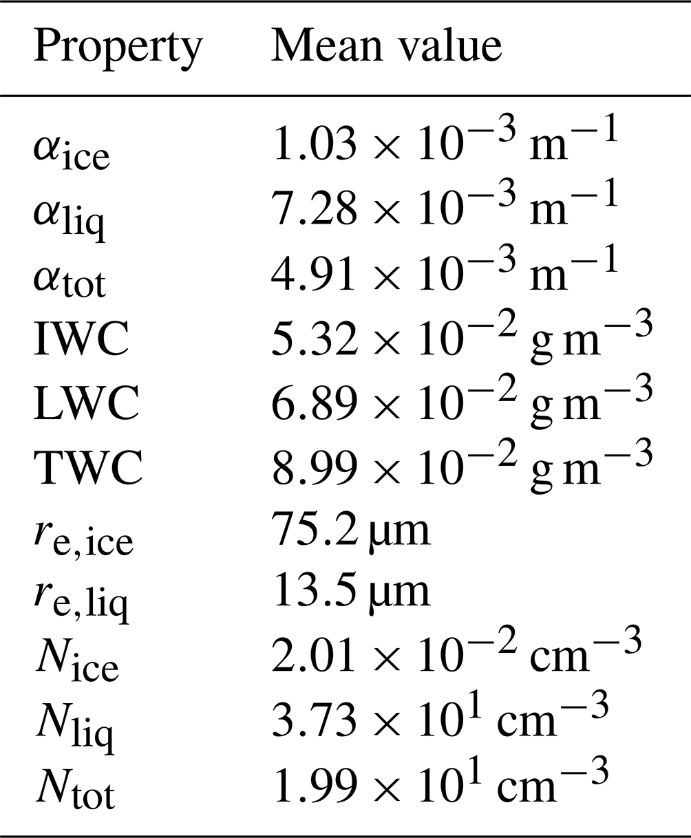
Table 7 presents the mean values in all selected pixels of all retrieved properties. These values allow us to observe trends for each variable. The extinction of the liquid droplets is stronger than that of the ice particles by a factor of 7. The same trends are observed between LWC and IWC with average values 30 % larger for LWC. The ice particles are larger than the liquid droplets by a factor of 5 for the mean values. The liquid number concentration is much higher than the ice number concentration by a factor of 10³. All retrieved variables can be compared with in situ measurements. For extinctions, water contents and concentrations, it is possible to sum the ice and liquid variables to obtain the total extinction α_tot (curtain in Fig. 4c), the total water content TWC (curtain in Fig. 5c) and the total number concentration N_tot (curtain in Fig. 7c).

Table 7 Mean values of retrieved properties.

3.3 Comparison

The retrieved total extinction of the mixed-phase layer is higher than that of the ice layer due to the presence of supercooled droplets. The extinctions from the CPI and FSSP have been summed in order to compare the sum with the total extinction of VarPy-mix and the one from the PN. These results are presented in Fig. 4c by the dots and share the same color scale as the VarPy-mix curtain. Above the cloud, where there is clear sky for VarPy-mix (coming from radar and lidar measurements and classifications), the PN detects no particles and the CPI + FSSP total extinction is very low (10⁻⁸ m⁻¹ for the FSSP). Inside the cloud we can observe the same trend between the VarPy-mix retrieval and the probe results, both of which are different mainly between the ice-only area and the mixed-phase layer.

In order to provide a more detailed comparison, we keep only the gates from VarPy-mix that are closest to the in situ measurements. Figure 4f displays by dots and lines the total extinction from the probes and from VarPy-mix. The points corresponding to the mixed-phase layer are highlighted in all panels by yellow and purple shading, and the others correspond to the ice cloud. Between 77.52 and 77.64° N in Fig. 4f, there are no data for VarPy-mix because these points correspond to a ground clutter (ocean) area for the radar. The extinction for the mixed phase is higher than for the ice cloud, and this trend is observed for all results. In general, VarPy-mix total extinction is lower than total extinction from probes, especially in regions where cloud-phase classification is defined as ice. In these regions the FSSP detects liquid droplets, whereas the CALIOP signal cannot be used because of the attenuation (extinguished). This may explain why α_VarPy is lower than α_CPI+FSSP.

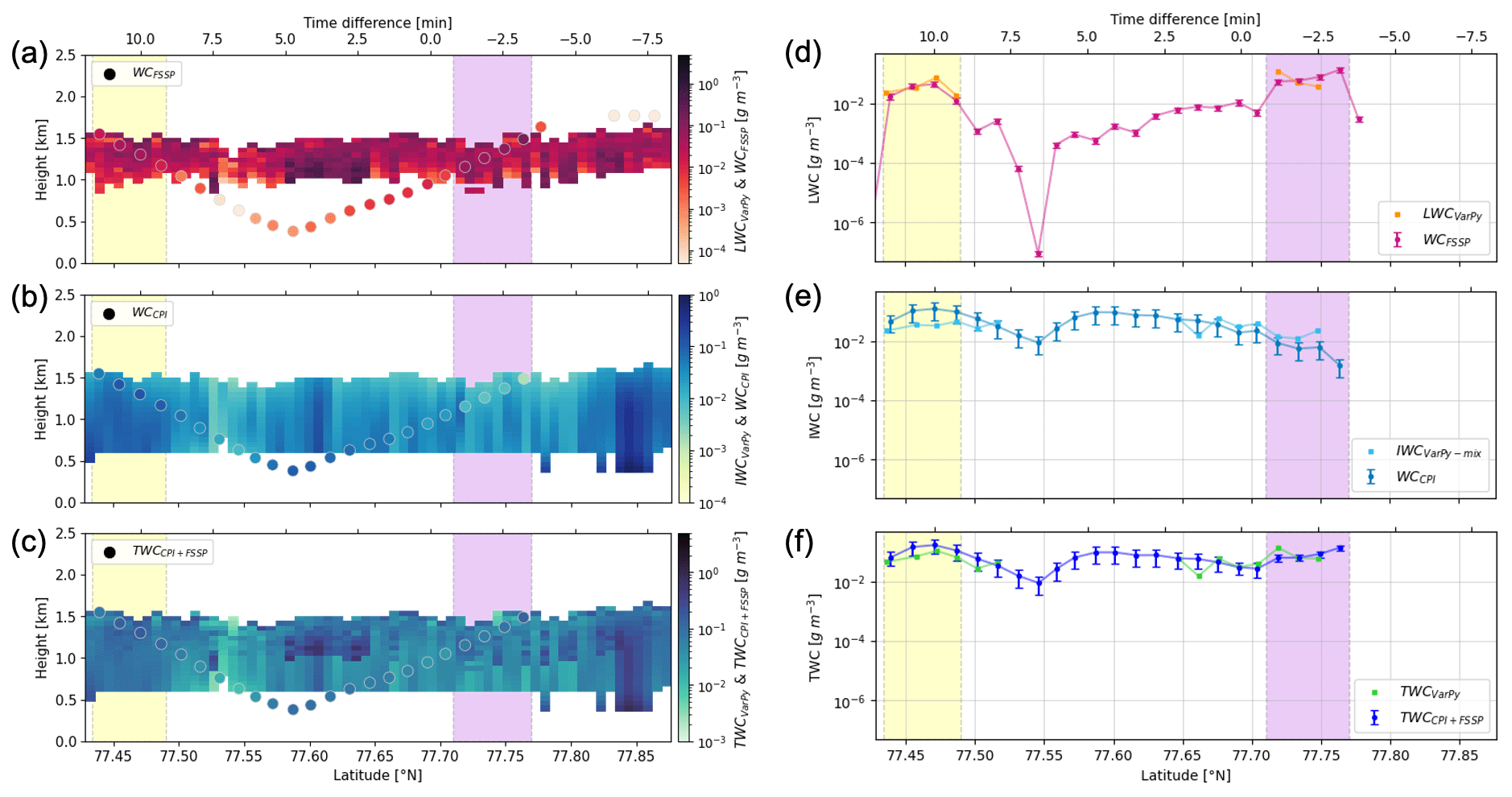
In the mixed-phase layer, IWC and LWC are both retrieved by VarPy-mix and can be compared with in situ data from the CPI and the FSSP, respectively. The TWC is also used in this comparison. The results are shown in Fig. 5. In both regions of mixed-phase measurements, the LWC retrieved by VarPy-mix is between $\mathrm{2}\times {\mathrm{10}}^{-\mathrm{2}}$ and $\mathrm{2}\times {\mathrm{10}}^{-\mathrm{1}}$ g m⁻³ and agrees well with the FSSP. Regarding IWC, both CPI and VarPy-mix retrieve similar trends in these regions. In the region below, due to the extinction of the lidar signal, only ice properties are retrieved by VarPy, but the FSSP also detects liquid in this region, which impacts the comparison with the TWC. For that reason we only compare in this region the IWC retrieved by VarPy-mix with the IWC from CPI, which are close to each other (40 % mean percent error). The region between 77.52 and 77.64° N cannot be compared for the same reason as for the extinction.

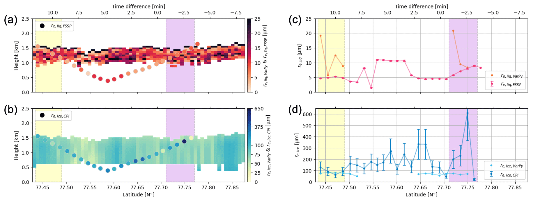
The same comparison between VarPy-mix retrievals and in situ measurements can be done for effective radii and concentrations, as is illustrated in Figs. 6 and 7, respectively. We can see in Fig. 6a and c that the liquid effective radius retrieved by VarPy-mix is higher than that from the FSSP. On the other hand, the ice effective radius from VarPy-mix is very close to the CPI effective radius in the mixed-phase layer indicated by the yellow shading (Fig. 6b and e). However, the values retrieved by VarPy-mix are much lower for the mixed-phase region indicated by the purple shading. In this region the CPI gives ice effective radii between 200 and 600 µm, while VarPy-mix retrieves values of around 70 µm. This difference may be due to the mass–size relationships applied, which differ between VarPy-mix and in situ data. Regarding the concentrations (Fig. 7), VarPy-mix retrieved fewer concentrated liquid particles than the FSSP and follows the same trend. For ice number concentration the values are lower for VarPy-mix in the mixed-phase layer indicated by the yellow shading and higher in the one indicated by the purple shading. In Fig. 7f the same trend as for the total extinction is obtained with higher values in the mixed-phase layer and very low values below it. The explanations are the same as for the extinction.

Table 8 Mean absolute error and mean percent error regarding in situ measurements for each property.

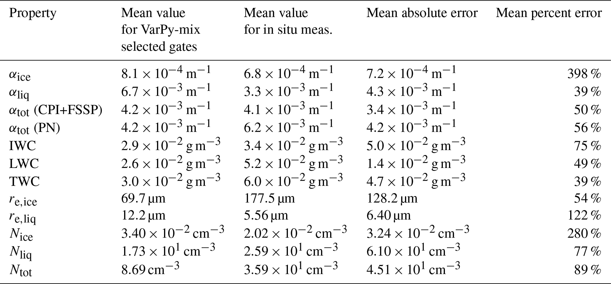
For all variables the mean absolute error (the mean of the absolute difference between each value of VarPy-mix and the in situ value) and the mean percent error regarding the in situ value (the mean of the absolute difference between each value of VarPy-mix and the in situ value divided by the in situ value and expressed as a percentage) are calculated and presented in Table 8. The liquid extinction retrieved by VarPy-mix differs from that in situ by 39 %, which is similar to in situ uncertainties (35 %), and is the closest to the in situ measurements. On the contrary, the mean percent error of ice extinction is 398 %. This can be explained by the large difference around 77.75° N, shown by the purple shading in Fig. 4e. The uncertainties in the in situ probes (Table 6) also need to be taken into account.

The comparison between VarPy-mix retrieval and the in situ measurements is limited for many reasons. First, the collocation in space is not perfect, which can lead to biases and restrict this study to one case. The Polar 2 aircraft flew almost exactly under the CloudSat and CALIPSO trajectories during the third leg by crossing them around 77.6° N. If we do not consider the measurement points above the clouds, the maximum spatial shifts are 1.68 km around 77.44° N and 1.34 km around 77.78° N. The temporal shift is also the best for the third leg with less than 10 min between the two platforms. Nevertheless, the sampling volumes of the probes are much smaller than those of the remote sensing instruments. Moreover, the vertical (60 m) and horizontal (1.4 km) resolutions of VarPy-mix products are larger than those of the probe sampling volume.

Another source of bias comes from the partial synergy of the VarPy-mix version in the mixed phase. Indeed, the retrieval relies more strongly on the a priori values than when both instruments are used to retrieve ice cloud properties (Delanoë et al., 2013). In addition, the ice cloud is mainly retrieved with radar only and therefore with a priori values, which are temperature-dependent. Furthermore, the main advantage of VarPy is the ability to retrieve full cloud profiles.

4 Summary and discussion

In this paper we propose a method to retrieve microphysical properties of ice, supercooled water and mixed-phase clouds simultaneously, called VarPy-mix. This variational method can use radar reflectivity at 35 or 95 GHz and lidar backscatter at 532 nm from spaceborne or satellite platforms to get vertical profiles of extinctions, ice and liquid water contents, effective radii, and number concentrations. Radar and lidar have different sensitivities to hydrometeors due to their wavelengths, and therefore this difference is used to retrieve the mixed phase. On one hand, lidar is very sensitive to small and highly concentrated particles such as liquid droplets. On the other hand, radar is sensitive to the particle size, meaning that the signal is stronger for ice particles than for liquid droplets. Consequently, ice clouds are retrieved with both instruments, while the mixed-phase retrieval is divided into two parts: the ice particles are retrieved with the radar signal and the supercooled water with the lidar signal. Therefore, the retrieval relies strongly on a priori and error values.

VarPy-mix is based on the algorithm Varcloud (Delanoë and Hogan, 2008), which retrieves ice cloud properties with radar, lidar and radiometric data. The variational method is the same, but the structure of the algorithm has been adapted to deal with supercooled water and mixed-phase clouds. The main modification comes from the state vector composition, which is divided into two parts, allowing ice and liquid to be processed separately as required. All matrices related to the state vector have been adapted to it. Moreover, a new lookup table dedicated to liquid properties has been created. Based on a log-normal droplet size distribution, it is used to retrieve supercooled water clouds and the liquid part of the mixed phase. For the ice clouds and the ice part of mixed-phase clouds, two lookup tables are implemented: one uses the T-matrix and the mass–size relationship from Heymsfield et al. (2010), and the second one is a combination of the mass–size relationships described by Brown and Francis (1995) and Mitchell (1996). It is important to know the phase of the cloud in order to process each gate appropriately. For this, an intermediate classification has been implemented. It distinguishes between ice clouds, supercooled water and the mixed phase. Adaptations have been made to this classification to improve the retrieval (reduce biases) and be consistent with the measurements.

The retrieved properties can be divided into two parts, with ice properties on one side and those of the liquid on the other. The results are vertical profiles of

• ice and liquid extinctions, α_ice and α_liq [m⁻¹], which can be used to estimate total extinction α_tot;

• ice and liquid water contents, IWC and LWC [kg m⁻³], which can be used to estimate total water content TWC;

• ice and liquid number concentrations, N_ice and N_liq [m⁻³], which can be used to estimate total number concentration N_tot;

• ice and liquid effective radius, r_e,ice and r_e,liq [m].

The case presented in this study is a mixed-phase layer on top of an ice boundary layer cloud at high latitudes. Therefore, ice and liquid properties are retrieved on top of the cloud and then ice properties for the ice cloud below. By comparing with in situ measurements from the ASTAR campaign, we can see that the cloud microphysical properties retrieved with VarPy-mix follow trends similar to those of in situ measurements and that the retrieval produces correct results. However, this comparison shows some limitations. First, the lower part of the cloud is missing, which compromises part of the comparison. In fact, the lidar is attenuated by the liquid droplets of the mixed-phase layer and extinguished after it. The radar does not detect down to the ocean because of the clutter and therefore cannot see the cloud base. Second, the spatial and temporal shifts between the aircraft and the satellites need to be taken into account, which are less than 1.7 km and 10 min, respectively, for the chosen case. Moreover, the sampling volume is not the same between in situ probes and CloudSat–CALIPSO (60 m vertical resolution). This makes it difficult to compare precisely a VarPy-mix gate with an in situ measurement. Third, the ice cloud retrieval is mainly done with the radar signal only, and each part of the mixed phase is also retrieved with a single instrument. The retrieval in this case relies strongly on a priori values and the lookup table, which includes some bias in the comparison with in situ measurements. A fully synergistic retrieval would be much more reliable, with both instruments retrieving each part of the mixed phase. Another possible improvement would be to optimize the a priori and first-guess values for liquid with in situ statistics. Moreover, it is important to note that the relationships used to retrieve properties differ between VarPy-mix and in situ measurements (e.g., the mass–size relationship to retrieve water contents). This has a particular impact on the comparison between ice effective radii. Finally, this study focuses on only one case of mixed phase at high latitude, above the ocean, which does not allow us to know how the algorithm would retrieve the mixed phase and the supercooled water globally.

In this study VarPy-mix is used to retrieve cloud properties with CloudSat and CALIPSO data. Nevertheless, it can also be applied to observations from other platforms. The French RALI airborne platform with the RASTA radar (95 GHz) and LNG lidar (multi-wavelength: 355, 532 and 1064 nm; high spectral resolution (HSR) at 355 nm) offers more possibilities for comparison with in situ measurements. During the RALI-THINICE campaign that took place in August 2022 near the Svalbard archipelago, the ATR42 from SAFIRE flew over and inside several mixed-phase cases, with RALI and in situ probes. VarPy-mix will be applied on RALI data, and some comparison with in situ measurements can be done to evaluate, validate and improve VarPy-mix parameterization. The same can be applied on other campaigns like HALO-(AC)³ (Wendisch et al., 2024), which took place in March and April 2022 in the Arctic near the Svalbard archipelago. During this campaign the HALO platform, consisting of the radar MIRA (35 GHz) and the lidar WALES (532 and 1064 nm and HSR at 532 nm) flew over mixed-phase clouds. Some collocation with aircraft performing in situ measurements was conducted during this campaign. More information on both campaigns can be found on their respective websites (RALI-THINICE, 2022; HALO-AC3, 2022). In addition, VarPy-mix could use data from the EarthCARE satellite platform, which was successfully launched on 28 May 2024 and includes cloud profiling radar (CPR) at 94 GHz and atmospheric lidar (ATLID) at 355 nm with HSR.