5 years of Sentinel-5P TROPOMI operational ozone profiling and geophysical validation using ozonesonde and lidar ground-based networks

The Sentinel-5 Precursor (S5P) satellite operated by the European Space Agency has carried the TROPOspheric Monitoring Instrument (TROPOMI) on a Sun-synchronous low-Earth orbit since 13 October 2017. The S5P mission has acquired more than 5 years of TROPOMI nadir ozone profile data retrieved from the level 0 to 1B processor version 2.0 and the level 1B to 2 optimal-estimation-based processor version 2.4.0. The latter is described in detail in this work, followed by the geophysical validation of the resulting ozone profiles for the period May 2018 to April 2023. Comparison of TROPOMI ozone profile data to co-located ozonesonde and lidar measurements used as references concludes to a median agreement better than 5 % to 10 % in the troposphere. The bias goes up to −15 % in the upper stratosphere (35–45 km) where it can exhibit vertical oscillations. The comparisons show a dispersion of about 30 % in the troposphere and 10 % to 20 % in the upper troposphere to lower stratosphere and in the middle stratosphere, which is close to mission requirements. Chi-square tests of the observed differences confirm on average the validity of the ex ante (prognostic) satellite and ground-based data uncertainty estimates in the middle stratosphere above about 20 km. Around the tropopause and below, the mean chi-square value increases up to about four, meaning that the ex ante TROPOMI uncertainty is underestimated. The information content of the ozone profile retrieval is characterised by about five to six vertical subcolumns of independent information and a vertical sensitivity (i.e. the fraction of the information that originates from the measurement) nearly equal to unity at altitudes from about 20 to 50 km, decreasing rapidly at altitudes above and below. The barycentre of the retrieved information is usually close to the nominal retrieval altitude in the 20–50 km altitude range, with positive and negative offsets of up to 10 km below and above this range, respectively. The effective vertical resolution of the profile retrieval usually ranges within 10–15 km, with a minimum close to 7 km in the middle stratosphere. Increased sensitivities and higher effective vertical resolutions are observed at higher solar zenith angles (above about 60°), as can be expected, and correlate with higher retrieved ozone concentrations. The vertical sensitivity of the TROPOMI tropospheric ozone retrieval is found to depend on the solar zenith angle, which translates into a seasonal and meridian dependence of the bias with respect to reference measurements. A similar although smaller effect can be seen for the viewing zenith angle. Additionally, the bias is negatively correlated with the surface albedo for the lowest three ozone subcolumns (0–18 km), despite the albedo's apparently slightly positive correlation with the retrieval degrees of freedom in the signal. For the 5 years of TROPOMI ozone profile data that are available now, an overall positive drift is detected for the same three subcolumns, while a negative drift is observed above (24–32 km), resulting in a negligible vertically integrated drift.

1 Introduction

Atmospheric ozone is an Essential Climate Variable (ECV) monitored in the framework of the Global Climate Observing System (GCOS). This is motivated by stratospheric ozone's decisive impact on the radiation budget of the Earth, while tropospheric ozone is the third most important anthropogenic contributor to greenhouse radiative forcing. Ozone, moreover, plays a central role in the oxidation chemistry of the atmosphere (Monks et al., 2015) and is an important air pollutant. Exposure to high levels of ozone can cause respiratory issues and be detrimental to health, vegetation, and materials. Studies related to atmospheric composition and the Earth's radiation budget therefore require accurate monitoring of the horizontal and vertical distribution of ozone at the scale of interest (WMO, 2010).

Atmospheric ozone concentration profile data records have been retrieved from backscattered solar ultraviolet (UV) radiation measurements by nadir-viewing satellite spectrometers since the 1960s, starting with the former USSR Kosmos missions in 1964–1965 (Iozenas et al., 1969) and NASA's Orbiting Geophysical Observatory in 1967–1969 (Anderson et al., 1969) and Backscatter Ultraviolet (BUV) on Nimbus 4 in 1970–1975 (Heath et al., 1973) and continuing with the Solar BUV series (SBUV(/2)) after 1978 (Heath et al., 1975). The Global Ozone Monitoring Experiment (GOME) in 1995–2002 (Burrows et al., 1999) paved the way to new-generation sounders including the SCanning Imaging Absorption spectroMeter for Atmospheric CHartographY (SCIAMACHY) on board ENVISAT (Bovensmann et al., 1999), the Ozone Monitoring Instrument (OMI) on the Earth Observing Satellite (EOS) Aura launched in 2004, the GOME-2 instruments on the Meteorological Operational (MetOp) satellites since 2006 (Munro et al., 2016; Hassinen et al., 2016), and the Ozone Mapping Profiler Suite (OMPS) nadir series started in 2011 (Flynn et al., 2006). Ensuring the uninterrupted continuation of this global monitoring of ozone and other trace gas concentrations is a requirement of the European Earth Observation Programme Copernicus (Ingmann et al., 2012). The Copernicus Space Component plans a series of three Sentinel-5 atmospheric composition missions, jointly developed by the European Space Agency (ESA) and the European Commission and to be operated by the EUMETSAT aboard its satellites MetOp-SG-A1 (Meteorological Operational – Second Generation), MetOp-SG-A2, and MetOp-SG-A3, scheduled in 2024, 2031, and 2038, respectively. As a gap-filler between the heritage satellites and the upcoming Sentinel-5 series, Sentinel-5 Precursor (S5P) was launched in October 2017 with the TROPOspheric Monitoring Instrument as a unique payload (TROPOMI; Veefkind et al., 2012).

Being the first atmospheric composition mission of the European Union's Copernicus Earth Observation Programme, the Sentinel-5 Precursor satellite is dedicated to the global atmospheric monitoring and study of air quality, climate forcing, ozone, UV radiation, and volcanic hazards. On board the S5P early-afternoon polar-orbiting satellite, the imaging spectrometer TROPOMI performs nadir measurements of the Earth's radiance from the UV-visible to the short-wave-infrared spectral ranges at a much finer spatial resolution than its predecessors do – and from which the global distribution of several atmospheric trace gases is retrieved daily, including stratospheric and tropospheric ozone. Developed at the Royal Netherlands Meteorological Institute (KNMI) and based on the optimal estimation method, TROPOMI's operational ozone profile retrieval algorithm has been implemented into the S5P Payload Data Ground Segment (PDGS), providing both near-real time (NRTI; for 50 % of the pixels by following a chequerboard pattern) and offline (OFFL) level 2 ozone profile data that are freely accessible from the Copernicus Data Space (https://dataspace.copernicus.eu/, last access: 26 June 2024).

Several scientific TROPOMI ozone profile retrieval products have been developed as well. First by Zhao et al. (2020), using an optimal estimation retrieval algorithm previously applied to GOME, GOME-2, OMI, and OMPS. Mettig et al. (2021) followed with the TOPAS (Tikhonov regularised Ozone Profile retrievAl with SCIATRAN) algorithm, which has also been used for joint UV–IR (infrared) retrievals from TROPOMI and the Cross-track Infrared Sounder on the Suomi National Polar-orbiting Partnership (CrIS/Suomi-NPP). A similar combination of TROPOMI UV and CrIS IR retrieval wavelengths has been exploited by the MUlti-SpEctra, MUlti-SpEcies, MUlti-SEnsors (MUSES) retrieval algorithm, which is a core part of the TRopospheric Ozone and its Precursors from Earth System Sounding (TROPESS) pipeline developed by Malina et al. (2022). An additional TROPOMI ozone profile product is currently under development at the Rutherford Appleton Laboratory (RAL, UK) within ESA's Climate Change Initiative (CCI) on ozone. It is based on the existing RAL UV-Vis processor (v2.14 to v3.01; see Keppens et al., 2018; Pope et al., 2023).

The first objective of this article is to provide an extensive description of the ozone profile retrieval processor currently used for S5P operational data processing (Sect. 2). This processor has also been used to back-process the entire TROPOMI level 1B version 2 data record, providing a homogeneous 5-year record of level 2 ozone profile data, denoted as L2__O3__PR version 2.4.0. The second objective of this work is to summarise the comprehensive quality assessment (QA) of this TROPOMI ozone profile data record, whereby results are collected from both the ESA/Copernicus Atmospheric Mission Performance Cluster's operational Validation Data Analysis Facility (ATM-MPC VDAF) and the S5P Announcement of Opportunity (AO) Validation Team (S5PVT) activity CHEOPS-5p. The QA approaches used are detailed in Sect. 3. They are based on the same validation practices as developed for and applied to the heritage sounders (Keppens et al., 2015, 2018). The validation methodology relies on the analysis of data retrieval diagnostics and on comparisons of TROPOMI data with co-located ground-based measurements used as a reference. The latter are acquired by ozonesondes contributing to the World Meteorological Organization's (WMO) Global Atmosphere Watch (GAW) and its data networks, by tropospheric lidars affiliated with the Tropospheric Ozone Lidar Network (TOLNet; Leblanc et al., 2018), and by stratospheric lidars affiliated with the Network for the Detection of Atmospheric Composition Change (NDACC; De Mazière et al., 2018). QA results are collected in Sect. 4. The dependence of TROPOMI's ozone profile information content and uncertainty on several influence quantities (like solar zenith angle and surface albedo) and measurement parameters (like the scan angle) is examined and discussed. This work concludes with an examination of the product compliance with mission requirements and consistency with other TROPOMI ozone retrievals, enabling data users to verify the fitness for purpose of the operational S5P ozone profile data. Conclusions are provided in Sect. 5, while some more detailed tables and figures are collected in the Supplement.

2 Operational TROPOMI ozone profiling

2.1 Instrument description and status

The TROPOspheric Monitoring Instrument is the unique payload on the Copernicus S5P satellite, the first atmospheric composition mission in the European Union Copernicus Earth Observation Programme (Ingmann et al., 2012). S5P was launched into a Sun-synchronous low-Earth orbit on Friday, 13 October 2017, and, with a foreseen mission lifetime of 7 years, is still fully operational today. The ascending node of the satellite orbit crosses the Equator at 13:30 local solar time. The four imaging spectrometers of TROPOMI measure the spectral radiance scattered at nadir from the sunlit part of the atmosphere and the solar spectral irradiance in the 270–2385 nm wavelength range at 0.2–0.5 nm resolution. The field of view at nadir produces ground pixels of 5.5 × 3.5 km² (along-track × across-track) since the pixel size switch of 6 August 2019 and of 7 × 3.5 km² before. The large swath width of 2600 km across-track produces a nearly daily coverage of the global (sunlit) atmosphere, with narrow gaps between orbits at the Equator. After spectral and radiometric calibration of the Earth radiance and solar irradiance data (Kleipool et al., 2018; Ludewig et al., 2020), operational data processors retrieve the total column abundance of several atmospheric trace gases related to air quality, climate, UV radiation, and environmental hazards. For ozone, a full vertical profile is retrieved.

2.2 Ozone profile retrieval algorithm

The operational TROPOMI ozone profile algorithm developed at KNMI derives the ozone concentration as a number density at 33 pressure levels throughout the atmosphere from the TROPOMI reflectance observations in the wavelength region between 270 and 330 nm, provided by bands 1 (267–300 nm) and 2 (300–332 nm) of the UV detector. In addition to the a priori ozone profile, the retrieved ozone profiles, and their errors, the following diagnostic information is provided: diagonal elements of the a priori error covariance matrix, a correlation length for the a priori errors, the a posteriori error covariance matrix, and the averaging kernel matrix (for the elements corresponding to the ozone profile). The ozone profile is also reported as six subcolumns with a vertical sampling of 6 km up to an altitude of 24 km and lower sampling above until the top of the atmosphere. The main elements of the retrieval algorithm are the forward model (Sect. 2.2.2), including the state vector and its derivative with respect to the fitted parameters, and the optimal estimation (OE) fitting (Rodgers, 2000), described in Sect. 2.2.4. Before the OE algorithm, several pre-processing steps are applied to the measured spectra (Sect. 2.2.1). The core of the algorithm is the OE method, which combines the information from the measured spectra with the a priori information and with the simulated reflectances computed with the forward-model calculations. A schematic overview of the algorithm is provided in Fig. 1. In this section, a brief overview of the main elements is provided, for a comprehensive description the reader is referred to the Algorithm Theoretical Basis Document (Veefkind et al., 2021).

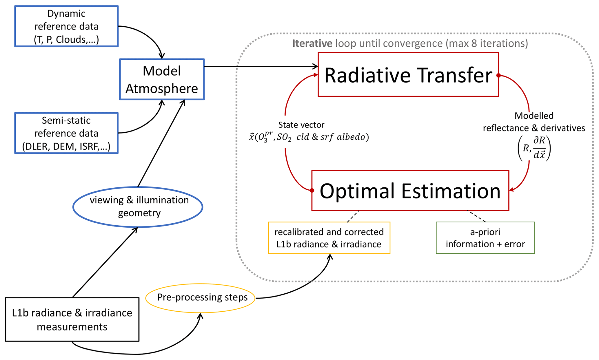
Figure 1 Schematic overview of the ozone profile retrieval algorithm. The main elements are the radiative-transfer calculations (the forward-model calculations), which provide the input modelled reflectance and its derivative to the optimal estimation method. The latter calculates the state vector with respect to the fitted parameters in the parenthesis. An iterative loop between these two elements (the light grey contour) is performed until convergence or the maximum number of eight iterations is reached.

2.2.1 Pre-processing

The pre-processing includes all the steps required to provide recalibrated radiance and irradiance spectra, corrected for polarisation and rotational Raman scattering (RRS) that are the inputs for the OE algorithm. It consists of spectral calibration, spectral and spatial regridding, correction for polarisation and RRS, and radiometric correction.

• Spectral calibration. The spectral calibration is performed only on the solar irradiance data using the precise knowledge of the Fraunhofer lines in the solar spectrum (van Geffen et al., 2022). A wavelength shift parameter is fitted on the irradiance spectrum for the spectral window (270–320 nm), while the assigned wavelengths from the L1B processor are used as is for the Earth radiance spectra.

• Spatial regridding. The ozone profile algorithm uses data from TROPOMI bands 1 and 2, both registered by the same UV detector (Kleipool et al., 2018; Ludewig et al., 2020). To suppress noise at shorter wavelengths, the band 1 data are measured at a lower spatial sampling in the across-track direction. For the ozone profile retrieval algorithm, the band 1 and band 2 data need to be spatially co-registered. Therefore, the radiance and irradiance data for the band 2 ground pixels are averaged to match the band 1 ground pixels. We compute the signal-to-noise ratio (SNR) of the averaged band 2 pixels, assuming that it is dominated by shot noise. Similar to the radiance and irradiance data, we also average the band 2 instrument spectral response function (ISRF) using the same procedure. After the regridding in the across-track direction, we average the radiances over five scan lines in the flight direction. After the spatial regridding, we have continuous radiance spectra in the fit window (270–330 nm) for 77 across-track ground pixels with a spatial resolution of 28 × 28 km² (across-track × along-track) in nadir after 6 August 2019 and 28 × 35 km² before that date.

• Spectral regridding. The spectra of TROPOMI band 1 and 2 have a very large spectral oversampling (ratio of spectral resolution and spectral sampling) of more than 6.9. The algorithm performs line-by-line radiative-transfer computations on the spectral grid of the measured spectra. To reduce the number of line-by-line calculations, three spectral pixels are averaged, resulting in an oversampling ratio of at least 2.3. Similar to the averaging in the spatial directions, the SNR is recomputed assuming shot noise, and the ISRF is averaged to take the effect of the spectral averaging into account.

• Signal-to-noise ratio. The final SNR is clipped to a maximum of 150, thus implementing a noise floor. This noise floor has been introduced to account for errors in the forward model that are larger than the noise and significantly improves the convergence of the algorithm.

• Polarisation and Raman correction. To be able to run the online radiative transfer in scalar mode and only account for elastic scattering, we apply a correction for polarisation and RRS. The correction is based on a large dataset for which we computed the spectra with and without these two effects. A neural network has been trained on this dataset to predict the correction factors as a function of wavelength, Sun–satellite geometry, surface albedo and pressure, and total ozone column.

• Radiometric correction. From comparisons to other satellite sensors, as well as to forward models, it is known that the on-ground calibration performed for TROPOMI bands 1 and 2 has a significant spectral- and viewing-angle-dependent bias. Also, the instrument shows significant optical degradation in the UV which is not fully corrected in the level 1b data. For this reason, a yearly correction (known as soft calibration) has been implemented which is based on a comparison of the measurements with forward-model results. The correction parameters are also updated yearly to follow the instrument changes over time due to its optical degradation. They are obtained using a combination of several observations covering different seasons during the year (always with orbits over the Pacific Ocean), and they are computed as a function of the wavelength, across-track pixel number, and radiance level. Pressure, temperature, and ozone profiles from the Copernicus Atmospheric Monitoring Service (CAMS) global analysis are used as inputs. Additionally, the CAMS ozone profiles are scaled to match the total ozone column derived from the OMPS total column data (McPeters, 2017). First, the surface albedo is fitted in a small spectral window (328–330 nm). Next, the fitted surface albedo is applied to the entire wavelength fit window (270–330 nm) for the forward-model calculations. Figure 2a shows the correction implemented per each year (red points), since the beginning of the TROPOMI mission in 2018 (orbit 4165) up to December 2022 (orbit 24482), for four ground pixels (15, 25, 45, and 65), at a specific wavelength = 290 nm. The red points represent the yearly correction computed by combining the black and light grey points of the same year. Figure 2b shows the radiometric correction computed per each year as a function of the wavelength and for two ground pixels, 25 (top) and 45 (bottom). The largest corrections are in the Fraunhofer lines, where the radiance signals are quite low. As can be seen in Table 1, for the period between the reactivation of the RPRO processing and the injection of soft-calibration file v2 (25 July 2022 to 15 January 2023), the previous version (v1) of the soft-calibration file is used. The difference between the two versions is that for v1 only DDS6 (sixth diagnostic dataset) orbits were used to compute the correction parameters (as they were the only available at the moment of computation), while for v2 a combination of DDS6 and OFFL orbits was used. It is worth mentioning that the DDS6 data are identical to the RPRO data, for all intents and purposes, so that the difference between the two soft-calibration files is mostly related to the higher statistics for v2.

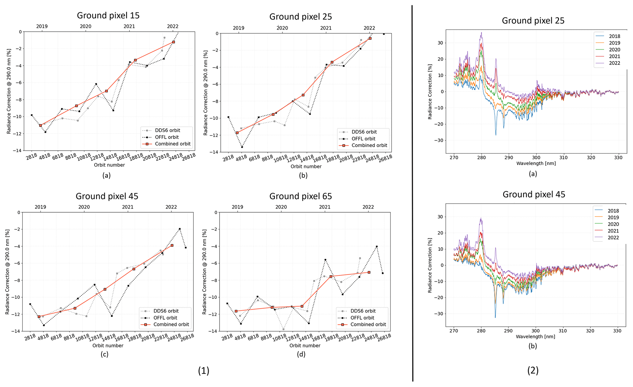
Figure 2 The yearly radiometric correction implemented from the beginning of the TROPOMI mission in 2018 up to December 2022 is shown in the four graphs, labelled (a) to (d) in panel (1), for four ground pixels (15, 25, 45, and 65) at a specific wavelength (290 nm). Panel (2) shows the radiometric correction per year (each line) as a function of the wavelength, for two ground pixels (25, panel 2a; 45, panel 2b).

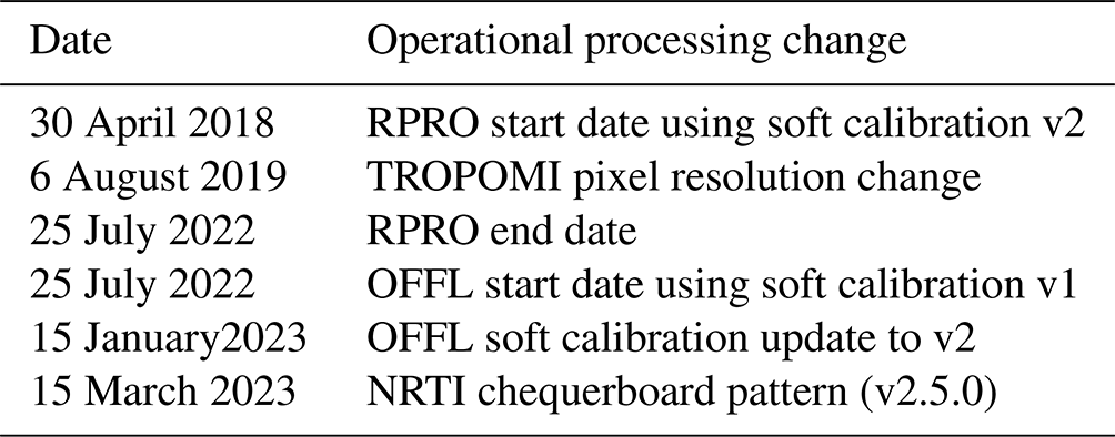
Table 1 Important changes in the operational TROPOMI ozone profile version 2.4.0 processing of near-real time (NRTI), offline (OFFL), and reprocessed (RPRO) data. The difference between the two soft-calibration versions is that for v1 only DDS6 (sixth diagnostic dataset) orbits were used to compute the correction parameters, while for v2 a combination of DDS6 and OFFL orbits was used.

2.2.2 Forward model

The forward model computes the Earth's reflectance for the Sun–satellite geometry of a ground pixel, at the spectral resolution of the observations, using the DISAMAR software (de Haan et al., 2022). As can be seen from the schematics in Fig. 1, the output of the forward model is the simulated reflectance that can be compared with the measured reflectance, as well as the derivatives with respect to the fit parameters, namely the ozone profile at 33 pressure levels, the SO₂ column, and the surface and cloud albedo (each at three wavelengths). The inputs of the forward model include, in addition to the model atmosphere parameters, the solar/viewing zenith and azimuth angles from the L1b data and the ISRF. The model atmosphere contains dry air, O₃, SO₂, and a Lambertian cloud, and it is bounded by a Lambertian surface. It is described by a pressure–temperature profile, the ozone profile, the SO₂ profile, the surface albedo, and the cloud albedo, fraction, and pressure. In the forward model, clouds are represented as Lambertian reflecting surfaces which cover part of the ground pixel and are placed at cloud pressure. The computations are performed with and without clouds, using the cloud fraction as a weight for partially clouded scenes. Cloud pressure and fraction are derived from the FRESCO algorithm using the oxygen A band of TROPOMI at 760 nm. Additionally, the cloud fraction and albedo are fitted at 330 nm during the retrieval of the ozone profile. The ozone profile is described as a number density at 33 pressure levels in the atmosphere. The atmosphere is assumed to be in hydrostatic equilibrium so that an altitude grid can be computed from the pressure–temperature profile. It is noted that the vertical grid for the model atmospheres is independent from the grid used for the radiative-transfer calculations. The radiative-transfer model used is based on successive orders of scattering using eight streams. The ozone absorption cross section is from Malicet et al. (1995), and the SO₂ cross section is a composite based on Bogumil et al. (2001) and Hermans et al. (2009).

2.2.3 A priori information

For all state vector elements, the OE method requires a priori values and their error estimates. The a priori information is based on the climatology of Labow et al. (2015), which provides the ozone profile and standard deviation as a function of latitude and total ozone column. This climatology has been adjusted by replacing the values in the troposphere and above the 0.1 hPa level with the median ozone profile for a given total ozone value to make the ozone profile independent of the ozone column for these pressure ranges. Forecast ozone columns from ECMWF are used to compute the a priori profile from the climatology. The errors in the a priori are based on the standard deviations provided by the climatology, but values are limited to the range of 20 %–50 %, while they are always set to 50 % for pressures larger than 250 hPa (i.e. lower altitudes). Additionally, a 6 km correlation length is used to compute the off-diagonal elements of the a priori error covariance matrix. The TROPOMI DLER (directionally dependent Lambertian-equivalent reflectivity; Tilstra, 2022) is used to derive the a priori surface albedo, while for the a priori cloud albedo the Fast Retrieval Scheme for Clouds from the Oxygen A band (FRESCO) is used. For cloud fractions below 0.2, the cloud albedo variance is set to 10⁻⁸, thus effectively fitting only the surface albedo. For cloud fractions above 0.2, the opposite is done, using an a priori surface albedo error of 10⁻⁸ and 1.0 for the cloud albedo error. For the SO₂ column, we use an a priori value of 0.01 DU and an a priori error of 0.1 DU.

2.2.4 Optimal estimation fitting

The OE method is used to retrieve the fit parameter values and their errors, assuming the availability of the a priori estimates and the a priori error covariance matrix. The OE method assumes Gaussian distributions for all errors. The cost function f_c that is minimised in OE retrievals is defined as follows (Rodgers, 2000):

$$\begin{array}{}\text{(1)}& \begin{array}{rl}{f}_{\mathrm{c}}\left(\mathit{y},\mathit{x},{\mathbf{S}}_{\mathit{ϵ}},{\mathit{x}}_{\mathrm{a}},{\mathbf{S}}_{\mathrm{a}}\right)& ={\left[\mathit{y}-F\left(\mathit{x}\right)\right]}^T{\mathbf{S}}_{\mathit{ϵ}}^{-\mathrm{1}}\left[\mathit{y}-F\left(\mathit{x}\right)\right]\\ & +{\left(\mathit{x}-{\mathit{x}}_{\mathrm{a}}\right)}^T{\mathbf{S}}_{\mathrm{a}}^{-\mathrm{1}}\left(\mathit{x}-{\mathit{x}}_{\mathrm{a}}\right),\end{array}\end{array}$$

where y is the vector of measured reflectance containing values for the different wavelengths. F(x) is the vector of calculated reflectances (the forward model). x is the state vector containing the parameters that are to be fitted. S_ϵ is the error covariance matrix of the measurement, which is diagonal here as the measurement errors are assumed to be dominated by shot noise and therefore uncorrelated. x_a is the a priori state vector. S_a is the a priori error covariance matrix. In Eq. (1), the a priori term is important for the retrieval stability. Updates to the state vector are based on the Gauss–Newton method, while the convergence criterion is based on Rodgers (2000, Sect. 5.6.3). After finishing the iterative loop, the output parameters are collected, and the O₃ subcolumns are computed by integrating the profile over the subcolumn altitude ranges. Also, quality flags are computed from the diagnostic information.

3 Quality assessment: approaches

The operational quality assessment of the TROPOMI ozone profile data by the ESA/Copernicus ATM-MPC applies the satellite validation protocol initially developed by Keppens et al. (2015) for the GOME-2, SCIAMACHY, and Infrared Atmospheric Sounding Interferometer (IASI) missions. It majorly entails (1) visual inspections of daily maps of S5P ozone data and associated parameters, (2) assessment of the retrieved information content based on the analysis of the averaging kernels associated with each retrieved pixel, and (3) comparisons to independent reference measurements collected from ground-based monitoring networks. Analysis is performed on the native vertical grid of the profile retrieval (33 levels; see Sect. 2), although the derived product consisting of six integrated ozone subcolumns is considered here as well.

The daily ozone and correlation checks for a selection of satellite data parameters within the orbit files are produced by KNMI using the PyCAMA software. Such checks provide a view on single-orbit features, correlations between retrievals of subsequent pixels, the appropriateness of the data flagging, etc. The daily results can be found on the TROPOMI MPC portal for level 2 quality control (https://mpc-l2.tropomi.eu, last access: 26 June 2024). For the routine comparative validation of the TROPOMI ozone profiles, the automated validation server (VDAF–AVS; https://mpc-vdaf-server.tropomi.eu, last access: 26 June 2024) deployed within the ATM-MPC VDAF automatically collects S5P ozone profiles and correlative measurements to identify suitable co-locations, compare the co-located data, and produce S5P data quality indicators. The VDAF–AVS produces curtain plots (ozone number density as a function of altitude and time) of the satellite data at a selection of ground-based ozonesonde and stratospheric lidar stations, together with curtain plots showing the difference between TROPOMI and the ground-based reference data. The VDAF–AVS also provides statistical estimates of the bias and dispersion of S5P data with respect to the ground-based measurements.

The TROPOMI Validation Data Analysis Facility additionally produces consolidated validation results through the versatile Multi-TASTE validation system developed and operated at BIRA-IASB (Lambert et al., 2014). These consolidated results, including both information content studies and comparisons with independent reference measurements (also see the next subsections), are the main focus in this work and discussed with respect to the TROPOMI product quality targets in the upcoming results sections. Summaries of past and future intermediate results can be found on the VDAF website (https://mpc-vdaf.tropomi.eu, last access: 26 June 2024) and in the quarterly TROPOMI MPC Routine Operations Consolidated Validation Report (ROCVR) through the same link.

3.1 Data selection for the present study

This work reports on the validation of 5 years of TROPOMI operational ozone profiles retrieval between 1 May 2018 (orbit 2818; actually dated 30 April 2018 in UTC) and 30 April 2023. These data originate from the chain of processors operated by TROPOMI's MPC, including L1B processor version 2.0 (except for 5 months at the end of 2022; see below) followed by the NL-L2 processor version 2.4.0 or 2.5.0 and are obtained from the former Copernicus Open Access Hub (https://scihub.copernicus.eu, last access: 29 September 2023), with collection number 03 combining offline (OFFL) and reprocessed (RPRO) data streams. Important dates and corresponding changes within this 5-year period are listed in Table 1. The near-real time (NRTI) stream differs hardly from the offline stream but follows a chequerboard pattern in its pixel selection since version 2.5.0 (starting on 15 March 2023), allowing more rapid data processing and delivery. Except for minor formatting changes, this reduction in sampling is the only difference between the 2.4.0 and 2.5.0 processors.

The operational TROPOMI orbit data files contain, for each individual ozone profile retrieval, the ozone number density on 33 pressure levels, the integrated tropospheric and total ozone columns, and 6 integrated subcolumns (0–6, 6–12, 12–18, 18–24, 24–32, and 32–82 km). For the validation activities presented here, we consider the station overpass pixels obtained from the MPC Payload Data Ground Segment in HARP format (v1.15, https://atmospherictoolbox.org/harp, last access: 26 June 2024). Data users are encouraged to read the product read-me file (PRF), product user manual (PUM), and algorithm theoretical basis document (ATBD) of this product, all of which are available online (https://sentiwiki.copernicus.eu/web/s5p-products, last access: 26 June 2024).

In order to avoid misinterpretation of the data quality, we follow the PUM recommendation to use only TROPOMI ozone profile retrievals with a QA value above 0.5, which includes screening of profiles with the solar zenith angle (SZA) > 80°. Another piece of diagnostic information which indicates the quality of the fit is the so-called cost function (f_c in Eq. 1) which is minimised during the optimal estimation retrieval. It is recommended to apply a screening to the retrieval values showing a cost function f_c larger than 200 (value determined from sensitivity studies). Moreover, to filter out retrieved ozone profiles (with number density values n) that deviate too strongly from their a priori profile (with values n_ap) for all 33 levels (denoted l) combined, an additional rejection criterion is applied as follows:

$$\begin{array}{}\text{(2)}& \sum _{l=\mathrm{1}}^{\mathrm{33}}\left|n\right(l)-n_{\mathrm{ap}}(l\left)\right|>{\mathrm{10}}^{\mathrm{13}}\mathrm{molec}.{\mathrm{cm}}^{-\mathrm{3}}.\end{array}$$

3.2 Information content and vertical sounding studies

The information content of the TROPOMI ozone profile data is assessed through algebraic analysis of the averaging kernel (AK) matrix that is associated with each profile retrieval and generated by the same processing algorithm. The row sums of the AK matrix indicate the vertical sensitivity of the ozone profile retrieval. The trace of the AK matrix gives the degrees of freedom in the signal (DFS) to be understood here as the number of vertical subcolumns with independent information in terms of Shannon information content (Rodgers, 2000). The full width at half-maximum (FWHM) of the AK corresponding to a given altitude is selected in this work as an indicator of the effective vertical resolution of the retrieved profile at this altitude, although it is determined independently of any vertical displacement of the kernel (Keppens et al., 2015). This effective resolution of the retrieved information is not the sampling resolution of the vertical grid used for the retrieval process, which usually oversamples the true physical resolution of the retrieved information. Finally, the effective altitude registration of the retrieved profile information at a given altitude is estimated as the barycentre or peak position of the associated AK at this altitude.

3.3 Comparisons with correlative reference measurements

TROPOMI ozone profile data are compared to ground-based reference measurements acquired by instruments contributing to WMO's Global Atmosphere Watch (GAW), the Network for the Detection of Atmospheric Composition Change (NDACC; De Mazière et al., 2018), Southern Hemisphere ADditional OZonesondes (SHADOZ; Thompson et al., 2019), and Tropospheric Ozone Lidar Network (TOLNet; Leblanc et al., 2018) using (1) balloon-borne ozonesondes, (2) tropospheric ozone differential absorption lidars (DIAL), and (3) stratospheric ozone DIAL. The first two reference instruments are used to assess the quality of TROPOMI profile retrievals in the troposphere and up to the middle stratosphere, while the latter is used as reference to validate the full stratospheric part of the TROPOMI ozone profile. The ground-based data are collected through ESA's Validation Data Centre (EVDC; https://evdc.esa.int/, last access: 26 June 2024), and the respective data host facilities of the ground-based networks. A global map showing all reference measurement stations considered in this work (60 ozonesondes, 4 tropospheric lidars, and 6 stratospheric lidars) is depicted in Fig. 3. The geographical distribution of the stations indicates the domain of applicability of the comparative validation results. The exact station locations and data sources are provided in Tables S1 to S3 in the Supplement.

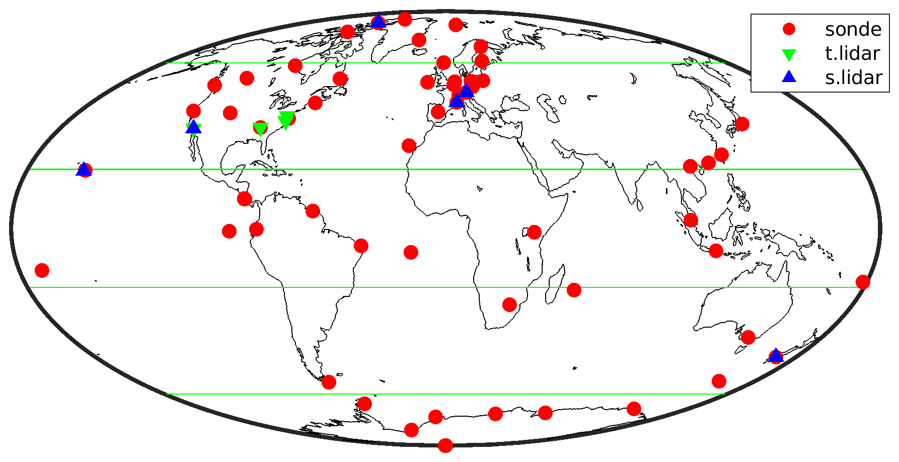
Figure 3 Geographical distribution of the ozonesonde, tropospheric (t.) lidar, and stratospheric (s.) lidar stations having coincident measurements with the S5P ozone profile data for the comparisons reported in this work. Horizontal green lines separate the five latitude zones that are distinguished in the comparative analysis with respect to ozonesondes.

3.3.1 Balloon-borne ozonesonde measurements

Launched on board small meteorological balloons, an electrochemical ozonesonde measures the vertical distribution of atmospheric ozone partial pressure from the ground up to burst point, typically around 30 km. Measurement errors depend on the type and the preparation of the sonde instrument (Smit, 2014; Stauffer et al., 2022), as well as on how the post-processing of the acquired raw data is done. When standard operating procedures are followed, systematic differences with respect to the reference photometer at the World Calibration Centre for Ozone Sondes (WCCOS) in Jülich are negligible with an uncertainty of up to 5 %. Except for the tropical upper troposphere, the random uncertainty is less than 3 %–5 % below 27 km (Smit et al., 2021). The ozonesonde data originate from the NDACC Data Host Facility, the SHADOZ archive, and the World Ozone and Ultraviolet Radiation Data Centre (WOUDC). Since their vertical resolution is much higher than that of the TROPOMI ozone profiles, they can also be used to estimate the vertical smoothing error in the remotely sensed profiles.

3.3.2 Differential absorption lidar measurements

Ozone differential absorption lidars (DIAL) can measure the vertical profile of ozone number density in the troposphere (500 m a.g.l. to 12–15 km) or in the stratosphere (8–10 to 45–50 km). Ground-based systems perform network operation in the framework of the international Network for the Detection of Atmospheric Composition Change (NDACC) and the North-American-based Tropospheric Ozone Lidar Network (TOLNet). For stratospheric measurements, the effective vertical resolution typically degrades with altitude from a few hundred metres at 10 to 3–5 km in the upper stratosphere, and the total uncertainty (systematic and random effects included) ranges from 4 % below 30 km to 10 % or more at 35 km and above (Leblanc et al., 2016). For tropospheric measurements, the effective vertical resolution also degrades with altitude from a few metres in the boundary layer to 2–3 km in the upper troposphere, and the total uncertainty ranges from 4 % (profile bottom) to 10 %–20 % (profile top). Between about 3 and 10 km, tropospheric ozone lidar measurements show a mean difference with the ozonesonde of less than 2 % and a root mean square deviation below 3 %, which are well within the combined uncertainties over the two measurement techniques (Leblanc et al., 2018). The MPC VDAF and its AVS make use of DIAL ozone profile data available through the EVDC, originating from the NDACC Data Host Facility, and through the TOLNet data archive.

3.3.3 Spatiotemporal co-location of data pairs

Comparisons between retrieved satellite pixels and reference measurements are based on unique spatiotemporal co-locations within 35 km and 12 h. This means every observation, whether by TROPOMI or a reference instrument, is considered in at most one comparison. The 35 km radius is chosen to have the ground-based reference measurement typically within the overpassing 28 × 28 km² satellite pixel, unless this pixel is flagged bad. In that case, the closest unflagged neighbouring pixel is picked. The ±12 h time window selects same-day (24 h period) observations for both daytime and nighttime measurements. Figure 4 displays the distribution of the temporal mismatch for all co-locations considered in this work. About 40 % of the ozonesonde co-locations and close to all tropospheric lidar measurements take place within 1 h of the satellite overpass. The ozonesonde profile time stamp is taken as the launch time for a few hours' flight, which is mostly taking place before local noon (positive satellite minus reference time). The DIAL time stamp is the middle of the minutes-to-hours measurement integration time window. This results in an 8 h difference on average for the nighttime stratospheric lidar observations that are mostly taking place before midnight the same day (negative time difference).

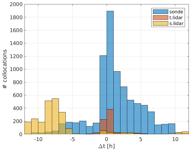
Figure 4 Histogram for the time differences (in hourly bins) between coincident TROPOMI and reference measurements, with ozonesondes in blue, tropospheric (t.) lidar in red, and stratospheric (s.) lidar in yellow. All bins add up to the co-location numbers in Fig. 11. Positive values indicate that TROPOMI measured later than the reference instrument.

3.3.4 Data harmonisation and comparison

The comparative validation of the TROPOMI ozone profiles with respect to reference measurements requires calculating difference profiles and hence the harmonisation of satellite and reference profiles in terms of physical quantities and vertical sampling at least (Keppens et al., 2019). The reference measurements are first converted to the altitude–number density representation, if needed, using auxiliary data that are provided with the ozone profile data (Keppens et al., 2015). Next, the reference measurements, which are acquired at higher vertical resolution than the TROPOMI profile data, are regridded to the satellite retrieval grid. This is achieved using a mass-conserving regridding approach, meaning that the integrated ozone column amount of each profile is conserved throughout the operation (Langerock et al., 2015).

Given that each retrieved ozone value shows an effective vertical position and resolution that differs from the retrieval grid (also see Sects. 3.1 and 4.3), the retrieved profiles come with a vertical smoothing error ${\mathit{ϵ}}_{\mathrm{V}}=\left(\mathbf{A}-\mathbf{I}\right)\left(\mathit{x}-{\mathit{x}}_{\mathrm{a}}\right)$, with A and x_a as the retrieval's averaging kernel matrix and prior profile, respectively. This vertical smoothing error is a systematic error that is correlated with the true state x and will therefore show variations on the same spatiotemporal scale as the actual ozone field. However, assuming the reference observations not to be vertically smoothed at all, the vertical smoothing difference error in the profile comparisons is only given by the satellite retrieval's vertical smoothing error ϵ_V. This means it can be accounted for by smoothing of the reference profiles x_r with TROPOMI's averaging kernels before comparison (Rodgers and Connor, 2003; Keppens et al., 2019):

$$\begin{array}{}\text{(3)}& {\mathit{x}}_{\mathrm{r}}^{\prime }=\mathbf{A}{\mathit{x}}_{\mathrm{r}}+\left(\mathbf{I}-\mathbf{A}\right){\mathit{x}}_{\mathrm{a}},\end{array}$$

which is indeed equivalent to correcting the profile's difference for the vertical smoothing (difference) error ϵ_V if the reference profile x_r is taken as the best and non-smoothed estimate of the true profile x: ${\mathit{x}}_r^{\prime }={\mathit{x}}_{\mathrm{r}}+{\mathit{ϵ}}_{\mathrm{V}}={\mathit{x}}_{\mathrm{r}}+\left(\mathbf{A}-\mathbf{I}\right)\left(\mathit{x}-{\mathit{x}}_{\mathrm{a}}\right)\equiv \mathbf{A}{\mathit{x}}_{\mathrm{r}}+\left(\mathbf{I}-\mathbf{A}\right){\mathit{x}}_{\mathrm{a}}$ for x≡x_r (Rodgers, 2000). After application of Eq. (3) to each reference profile, making use of the co-located satellite profile's averaging kernel matrix and prior profile, the difference in satellite and reference ozone number density values is calculated for a selection of influence quantities.

Chi-square tests (${\mathit{\chi }}^{\mathrm{2}}=\mathrm{\Delta }{\mathit{x}}^T{\mathbf{S}}_{\mathrm{\Delta }}^{-\mathrm{1}}\mathrm{\Delta }\mathit{x}$) are added to all difference calculations. They allow verifying whether the observed differences Δx between the satellite and reference profiles are consistent with the ex ante (predicted) uncertainties over the difference S_Δ (von Clarmann, 2006; Keppens et al., 2019). The latter contains the satellite and reference covariances and uncertainties that are due to sampling, smoothing, and retrieval differences. By an application of the vertical averaging kernel smoothing, however, retrieval differences including vertical sampling and smoothing differences are essentially removed from the difference covariance (Keppens et al., 2019). This means that for the results presented here the difference covariance mainly contains the ex ante satellite and reference covariances. Horizontal and temporal sampling and smoothing differences are moreover minimised by application of the strict co-location criteria (see the previous subsection).

4 Quality assessment: results

4.1 Data content studies

The TROPOMI MPC quality control portal creates daily global maps of the six partial columns provided in the ozone profile product, together with the integrated total column. The latter is compared with the daily global map of the TROPOMI total column retrieval to assess their mutual consistency. Daily global maps easily allow identifying data gaps, retrieval and data screening artefacts, along-orbit striping, and other large-scale features that are not typically detected through comparison with respect to point-like ground-based reference data. The monthly mean of the six ozone profile subcolumns for October 2020 is shown in Fig. 5a–f. Each panel shows the main layer features; for example, in the first subcolumn from 0 to 6 km in Fig. 5a, the low-ozone levels highlight the Himalaya mountain range in Asia and the Andes mountain range in South America, while in the fifth subcolumn from 24 to 32 km in Fig. 5e, the stratospheric ozone layer is clearly visible. Note that in the absence of clouds, data files sometimes contain negative surface albedo values. The TROPOMI ground pixels affected by this anomaly are usually located at the east and west edges of the across-orbit measurement swath. For now, these negative values are set to zero in the radiative-transfer code and validation tools (as an influence quantity) but not in the ozone profile data distribution to users. In addition, Fig. 5g shows a 5 d average on 10–15 October for the 0–6 km layer. The map contains a cloud filter to only look at cloud-free scenes (cloud fraction below 0.2) and clearly shows some regions with higher-ozone levels in eastern Europe and reduced columns over the Alps and the Pyrenees.

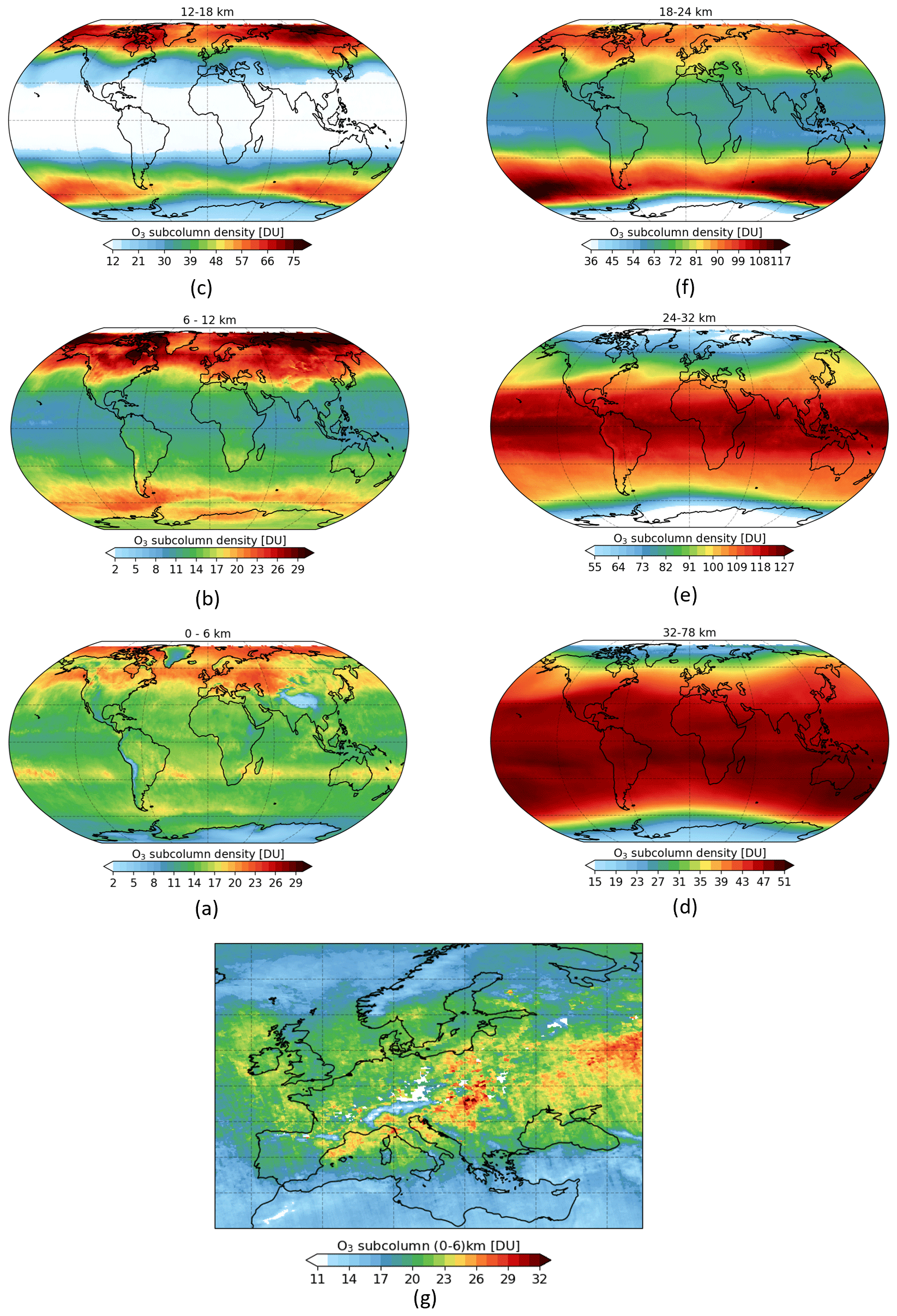
Figure 5 The mean ozone content in the six subcolumns of the ozone profile for the month of October 2020, during the ozone hole condition, is shown in panels (a) to (f), starting from the near-surface subcolumn (0–6 km). In panel (g), a 5 d (10–15 October) average of the ozone content in the lowest layer over Europe is shown. The colour scale is optimised per each subcolumn.

A comparison between the a priori ozone profile and the retrieval is shown in the zonal averages in Fig. 6 for 2 d in 2020, namely one in spring, when there is the highest amount of ozone, and one during the ozone hole season. Profiles are flagged bad if this difference exceeds the criterion in Eq. (2), which typically occurs towards the edge of the swath, i.e. for high viewing zenith angles. Figure 6 clearly shows how the measurements combine with the a priori values in a smoother retrieved ozone layer at the top panel. Moreover, the vertical sensitivity shown at the bottom indicates that the measurements add more information with respect to the a priori in most of the vertical layers, with low-sensitivity areas depending on the latitude (as also shown in Fig. 11). Figure 7 shows the percentage of retrieved pixels with good quality after filtering out those pixels with QA < 0.5, cost function > 200, and the prior condition expressed by Eq. (2) applied in this specific order. Each line represents the average of the same orbit number over all the days of the specific month (March, July, October, or December). The orbits are numbered in ascending order from left to right, as shown on the right-hand side of Fig. 7. There is a slight seasonal dependence, which also changes over the years. The daily variation shows a distinguished minimum around orbit 9–10 when TROPOMI passes over the South Atlantic Anomaly. This is more visible in the months of March, July, and October, while it does not have a large effect in December. In the Supplement, Fig. S1 shows the percentage trend of each separate filter applied in the same 4 months. The first two filters (QA and cost function) behave similarly, while the condition in Eq. (2), in the third column, rules out only a small percentage, as expected.

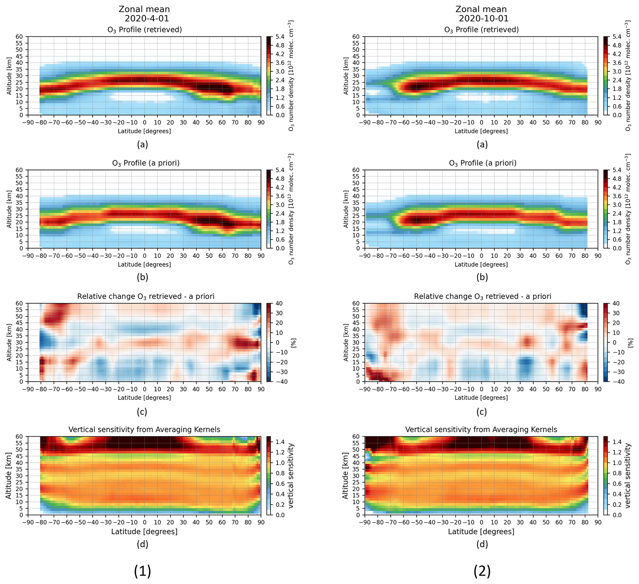
Figure 6 Zonal average of the ozone profile retrieval (a), the a priori ozone profile (b), their relative difference (c), and the vertical sensitivity (d) for 2 d in 2020, namely 1 April (first column, 1) and 1 October (second column, 2).

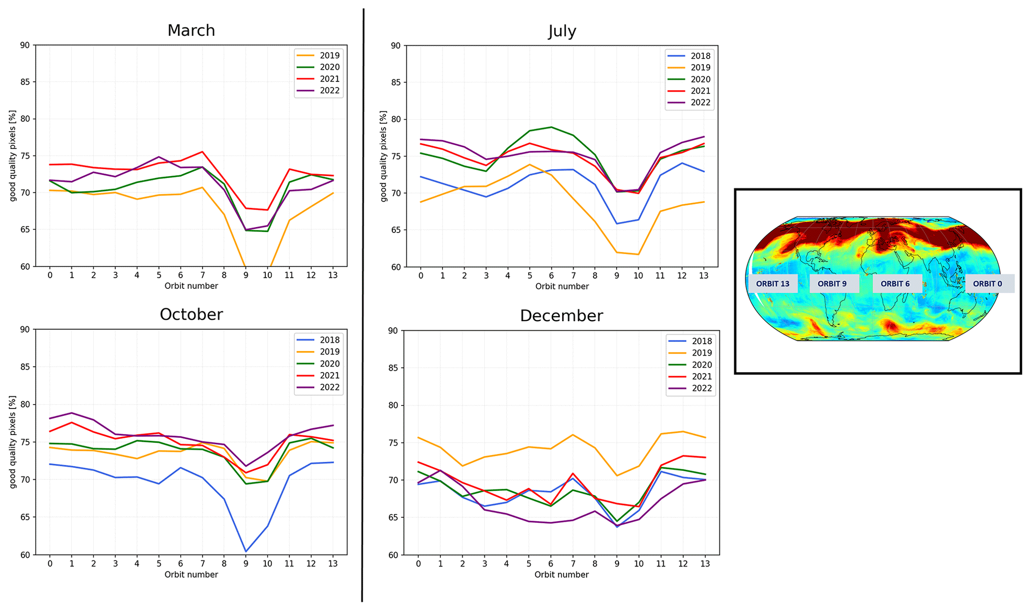
Figure 7 The percentage of good-quality pixels after applying the recommended filters on the QA value, cost function, and the condition in Eq. (2). Each line represents the average percentage of the same orbit number over all the days of the specific month analysed. To the right, the order of the orbits number is shown.

4.2 Vertical sensitivity and independent information

The information content of the TROPOMI ozone profile data is assessed through the analysis of the averaging kernel matrices. The retrieval's DFS as a measure of the number of independent pieces of information is given by the matrix trace. The monthly mean DFS of the ozone profile is shown in Fig. 8 for October 2020, during the ozone hole season. It shows a high correlation with the amount of ozone (and hence with latitude) as can be expected for an OE retrieval; higher-ozone amounts yield higher spectral signals and therefore have a positive impact on the retrieval sensitivity. Overall, the retrieved information on ozone is distributed over five to six vertical subcolumns of independent information showing about 5.5 on average, with values closer to 6 in the mid-latitudes and values just above 5 in the tropics and towards the poles.

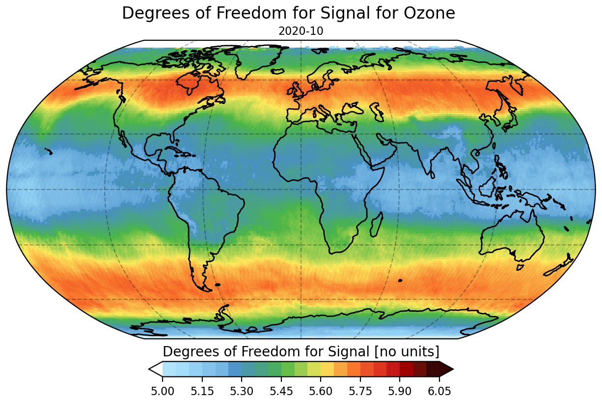
Figure 8 The monthly mean of the ozone degrees of freedom in October 2020.

The ozone retrieval DFS are also assessed for the six subcolumns provided in the TROPOMI ozone profile product separately. Figure 9 shows the correlation between each subcolumn DFS and ozone amount (first column). Subsequent plot columns show the layer DFS as a function of latitude and time (and solar zenith angle, viewing zenith angle, cloud fraction, and surface albedo in Fig. S2), including the subcolumn DFS mean and quantiles. First, it is clear that the six provided ozone subcolumns do not match the five to six pieces of information in the retrieval. The highest column (32–82 km; top row) roughly has 3 DFS, the column below (24–32 km) has 1 DFS, then two columns (12–18 and 18–24 km) each have about 0.5 DFS, and finally the lowest columns have 0.3 and 0.2 DFS from 6–12 and 0–6 km (bottom row), respectively. Together, these indeed add up to the average of 5.5, but significant deviations can be observed, especially as the 12–18 km subcolumn DFS highly correlates with its ozone amount (R = 0.8) and the solar zenith angle, resulting in a strong meridian dependence as well. A similar but much reduced meridian dependence is seen for the two adjacent subcolumns, while the correlation with ozone, SZA, and latitude becomes slightly negative for the lowest column and for the highest column for high solar zenith angles in combination with high surface albedos. The latter typically occurs for retrievals above Antarctic sea ice, which, due to the S5P orbit inclination, usually take place towards the left end of the swath, as can be seen from the viewing zenith angle dependence.

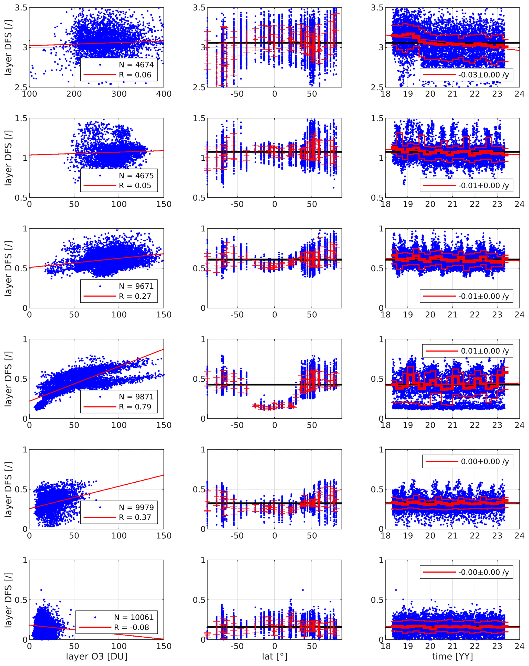
Figure 9 Correlation (R) between the six subcolumn DFS values and the six ozone subcolumns (bottom row to top row: 0–6, 6–12, 12–18, 18–24, 24–32, and 32–82 km) for N retrievals by TROPOMI (first column). Subsequent columns show the layer DFS as a function of latitude and time. Quantiles at 84 %, 50 %, and 16 % are added in red (per station or per season, with a thicker line for the median), together with the overall layer mean (black line). Yearly drifts are added to the temporal dependence plots.

Yearly drift values that are calculated from a linear fit are added to the temporal dependence plots in Fig. 9. The 2σ uncertainties over these values result from a bootstrapping technique with 1000 samples (Efron and Tibshirani, 1986). A DFS or retrieval sensitivity degradation is essentially non-existent for the lowest three subcolumns. The three columns above, however, show a degradation of just below 0.01 DFS per degree of freedom per year, corresponding to a 5 % DFS decrease over the 5-year period for the full profile. The vertical distinction in this degradation is in agreement with the typically stronger degradation towards the shorter UV wavelengths used primarily for the stratospheric ozone retrieval. The degradation of the longer wavelengths, relevant for the retrieval of tropospheric ozone, is less pronounced and hardly affects the corresponding DFS.

The vertical sensitivity of the S5P ozone profile data, determined by the averaging kernel matrix row sums, is assessed from the plots in Fig. 6 (bottom row) and Fig. 11 (fourth graph in each plot). On average, it nearly equals unity at all altitudes from about 20 up to 50 km, meaning that the information in the retrieved product fully originates from the TROPOMI observation. However, the sensitivity decreases rapidly at altitudes below 10 and above 50 km. Around the tropopause between 10 and 20 km (and around 25 and 50 km for high SZA), an over-sensitivity larger than 1 can be observed, which is a rather typical compensating effect for the under-sensitivity below (and above) in nadir profile retrievals. This over-sensitivity seems to be more pronounced and vertically expanding for higher solar zenith angles and again correlates with higher-ozone concentrations. As a result, the retrieved ozone below about 24 km will also show seasonal and meridian dependencies in its comparison with reference observations (see the next sections). The vertical sensitivity usually drops below 0.5 towards the surface, meaning that the majority of the information in the lowest subcolumn originates from the prior profile, rather than from the spectral satellite measurement.

4.3 Vertical sounding accuracy

The vertical sounding accuracy of the S5P ozone profile retrieval is assessed through the analysis of individual averaging kernels. The kernel peak position and width provide measures of the effective vertical retrieval altitude and resolution, respectively. When the retrieval information barycentre of an AK differs from the nominal retrieval altitude (Keppens et al., 2015), an offset different from zero is observed in the fifth graph in each plot of Fig. 11. In this work, the effective retrieval resolution is estimated from the kernels' FWHM and plotted for all co-located kernels in each sixth graph of Fig. 11. Note that jumps can occur in both quantities due to the finite retrieval grid.

The altitude registration of the retrieved profile information usually is close to the nominal retrieval altitude in the 20–50 km altitude range, i.e. the offset is nearly zero. Yet the retrieval shows increasingly positive and negative offsets below and above the 20–50 km altitude range, respectively, which can reach 20 km towards the surface. This means the majority of the retrieved surface ozone information (ignoring the prior contribution) comes from the UTLS (upper troposphere to lower stratosphere), in agreement with the occurrence of a sensitivity peak at that altitude. The direction of the offset is always towards higher retrieval sensitivities, i.e. positive for the troposphere and negative for the highest altitudes.

The effective vertical resolution of the TROPOMI ozone profile retrieval usually ranges within 10–15 km, with an optimum close to 7 km in the middle stratosphere (around 30–40 km). Better effective vertical resolutions (reduced kernel FWHM) can be observed for higher solar zenith angles (sideward atmospheric irradiation) in the troposphere and higher stratosphere, as can be expected for nadir (ozone) profilers. On the other hand, the kernel width becomes ill-defined for the very broad averaging kernels that originate from tropospheric level retrievals at lower solar zenith angles (as is the case for all tropospheric lidar comparisons in this work). With only one retrieval degree of freedom up to about 18 km (lowest three subcolumns in the previous section), the retrieved information is indeed very much vertically smeared, and a large part of the tropospheric ozone information comes from the prior profile. The low-SZA retrieval therefore goes hand in hand with increased vertical smoothing errors, as discussed in detail in Sect. 4.5 with respect to the uncertainty validation.

4.4 Comparison results

Figure 11 contains all comparisons between TROPOMI ozone profiles and reference data, with the latter AK-smoothed using Eq. (3), and corresponding statistics. Included are level-specific chi-square tests, which are discussed in the next section, and the information content diagnostics that facilitate the interpretation of the comparison results. The S5P ozone subcolumn comparisons in Figs. 10 and S3, on the other hand, are only with respect to vertically integrated ozonesonde measurements, again with preceding averaging kernel smoothing. Compared to ozonesonde and tropospheric lidar data, the S5P RPRO/OFFL data have a mean bias below ±5 %–10 % in the troposphere (in black). This is slightly lower than the mean prior profile bias (in white), although the reduced sensitivity towards the surface indicates that a significant part of the retrieved information originates from the a priori assumptions. In the stratosphere up to 35 km, stratospheric lidar data comparisons conclude to a mean bias of ±5 %–10 % as well. The bias goes up to −15 % above (35–45 km), but with vertical oscillations (positive and negative), and hence exceeds the mean prior bias around 40 km. These oscillations of the bias may be due to a typically larger a priori error in the mid- and high stratosphere (above 20 %) in comparison with other retrievals. S5P data comparisons with ozonesonde and stratospheric lidar data show a dispersion of order of 30 % in the troposphere and 10 % to 20 % in the UTLS to upper stratosphere.

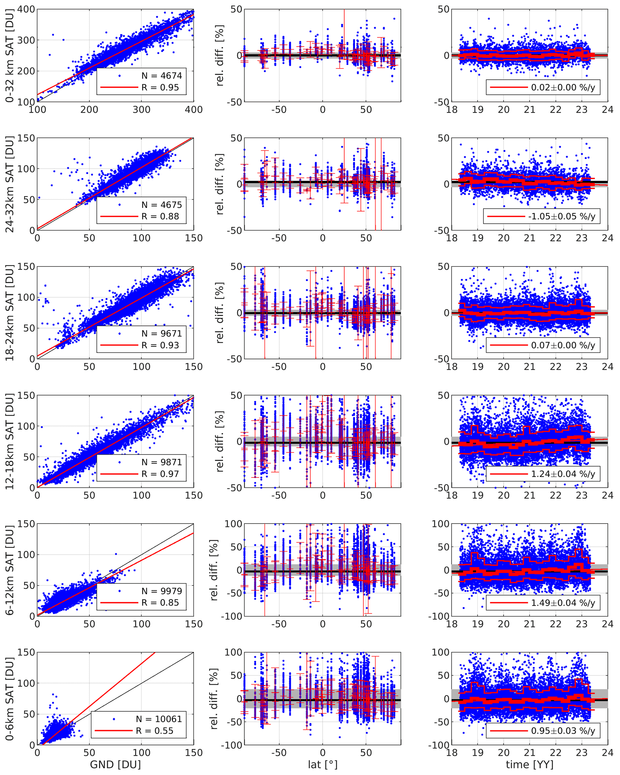
Figure 10 Correlation (R) between N lowest five ozone subcolumns (bottom row to second row: 0–6, 6–12, 12–18, 18–24, and 24–32 km) as observed by TROPOMI and the coincident vertically integrated ozonesonde measurements (first column) and their overall sum (top row, 0–32 km). Subsequent columns show the differences between satellite and ozonesonde subcolumns as a function of latitude and time. Quantiles of 84 %, 50 %, and 16 % are added in red (per station or per season, with a thicker line for the median), together with the overall mean difference (black line), and the product requirements for each subcolumn (grey areas). Yearly drifts are added to the temporal dependence plots.

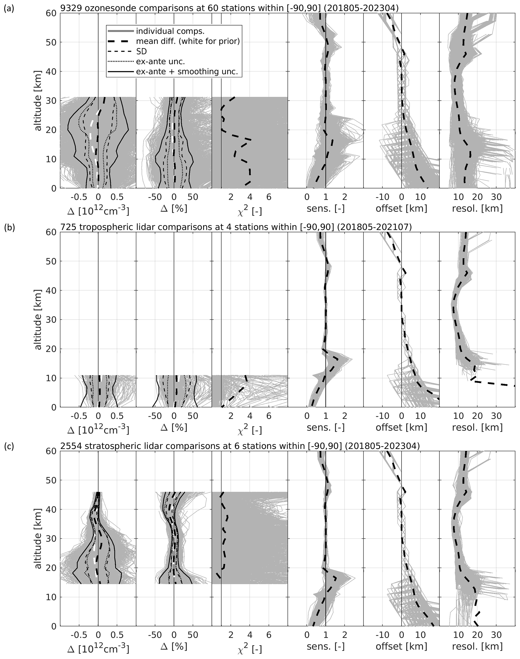
Figure 11 Comparison between S5P RPRO/OFFL ozone number density profile data and all co-located ground-based reference measurements. Every panel shows six graphs, respectively, from left to right: the difference and the percent relative difference between S5P and ozonesonde (a), tropospheric lidar (b) or stratospheric lidar (c), the chi-square (χ²) profile, the vertical sensitivity, the altitude registration offset, and the averaging kernel FWHM associated with the satellite retrieval. Grey lines show the individual comparisons. Dashed black lines show mean values (thick lines) and standard deviations (thin lines; around the mean), while dashed white lines indicate the mean difference between the a priori profile and the reference measurement. Dotted black lines indicate the total ex ante (inductive) uncertainty about TROPOMI and the reference measurements combined (around the mean difference). The black solid lines show the same, after adding the retrieval's smoothing error.

An optical path length dependence of the TROPOMI bias is observed for the subcolumns, which also translates into a seasonal and meridian dependence of the bias, as seen in Fig. 10. Scatterplots in the Supplement show the dependence of the subcolumn DFS (Fig. S2) and bias (Fig. S3) on SZA, VZA (viewing zenith angle) (both related to path length), cloud fraction, and surface albedo. The bias is clearly negatively correlated with the surface albedo for the lowest three subcolumns, despite the albedo's apparently slightly positive correlation with the retrieval DFS. The meridian dependence of the full profile bias with respect to ozonesondes is shown in Fig. S4 for five latitude bands, where increased tropospheric biases are observed for high solar zenith angles in the mid- to high latitudes. As a result, increased biases are found for high-SZA observations above highly reflective scenes, as is the case for Antarctic (sea) ice. On the other hand, when the deviation from the prior profile becomes too strong, these observations are flagged by the check in Eq. (2).

For the 5 years of TROPOMI RPRO/OFFL ozone profile data that are considered in this work, comparisons with the ozonesonde data reveal a positive drift for the lowest three subcolumns (0–18 km) and a negative drift of similar size for the 24–32 km subcolumn, while the drift is negligible for the subcolumn in between (18–24 km). The 6–12 km subcolumn shows the highest temporal difference change, with a positive drift close to 8 % over the 5-year period, which is also caused by higher positive biases in 2022 and early 2023. Overall, no drift is found for the profile integrated from 0 to 32 km (upper row in Fig. 10). More detailed, meridian drift assessments are shown in Fig. 12. These plots show robust linear regression results for the temporal dependence of the TROPOMI bias with respect to ozonesonde measurements (again on the retrieval grid). The horizontal bars indicate 2σ uncertainties over the drift from a bootstrapping technique with 1000 samples (Efron and Tibshirani, 1986). The significant positive and negative drifts that were observed for the subcolumns on the global scale are confirmed here for the tropics and mid-latitudes, with values up to 2 % yr⁻¹–3 % yr⁻¹ below 20–25 km and minus 1 % yr⁻¹–2 % yr⁻¹ above. No significant tropospheric drifts are detected towards the poles.

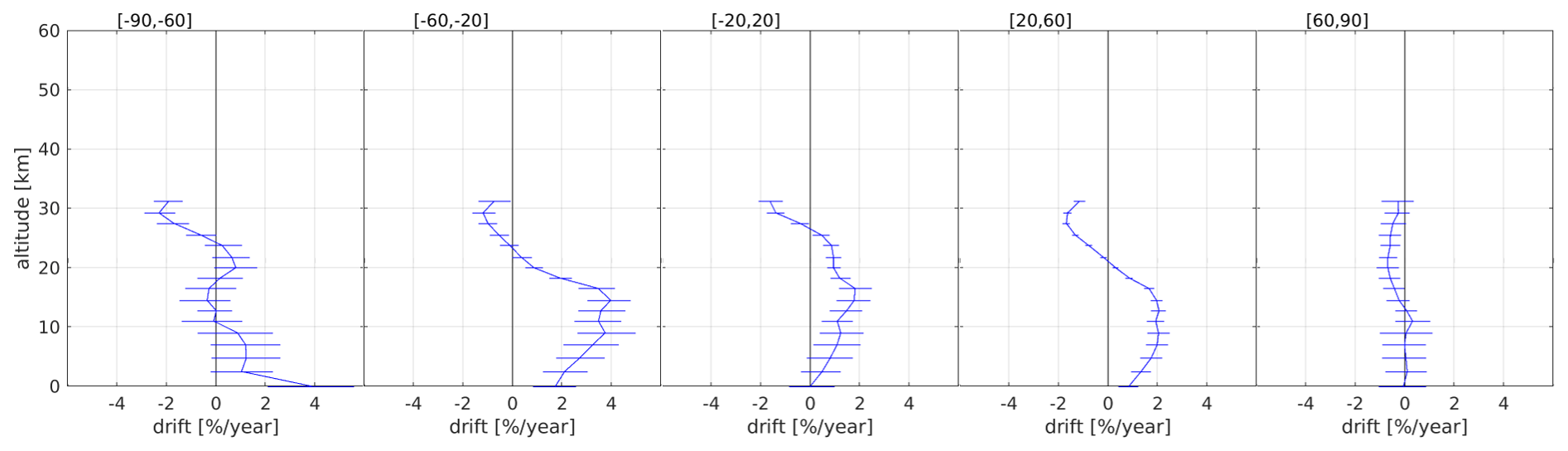
Figure 12 Altitude-dependent yearly TROPOMI ozone profile drifts determined from the ozonesonde comparisons and divided into five latitude bands. Horizontal 2σ error bars result from bootstrapping with 1000 samples.

4.5 Validation of uncertainty estimates

The validation of uncertainty estimates essentially consists of verifying the coherence of the ex ante (prognostic) retrieval uncertainty estimates using chi-square tests (Rodgers and Connor, 2003). These are here performed after strict co-location and averaging kernel smoothing, meaning that spatiotemporal sampling and smoothing difference errors are mostly corrected for. The retrieval's vertical smoothing error, although corrected for by the kernel smoothing operation, is here discussed in comparison with the total ex ante uncertainty in order to have a view of its typical (average) magnitude.

The chi-square plots in Fig. 11 (third graph in each plot) demonstrate that the observed differences confirm (χ² close to 1) the combined ex ante satellite and ground uncertainty estimates in the stratosphere on average, despite the appearance of large outliers. However, around the tropopause and below (around 15–20 km and lower), the mean chi-square value increases up to about 4 for both ozonesondes and tropospheric lidars, with especially high values for the tropics (low SZA) and Antarctic (high SZA and surface albedo) (see Fig. S4). Here, the prognostic (random) satellite uncertainty seems underestimated by a factor of 2, assuming correct reference uncertainties as discussed in Sect. 3.3. This can also be seen in the difference plots, as the dashed thin lines representing the dispersion of the difference are further away from the mean difference than the dotted lines representing combined ex ante uncertainties. Adding the smoothing difference error to the latter results in the solid thin black lines, pointing at values that are typically 10 %–30 % higher. The largest smoothing errors (up to 50 %) occur in the UTLS and towards the surface (where kernel edge effects are also at play).

4.6 Compliance with mission requirements

TROPOMI mission requirements have initially been expressed in the Science Requirements Document (SRD; Sentinel-5 Precursor Team, 2008) and the Geophysical Validation Requirements document (GVR; Sentinel-5 Precursor Team, 2014) and have later been reproduced in the TROPOMI validation plans and the product-specific ATBD (Veefkind et al., 2021). The SRD focuses on accuracy requirements for the integrated subcolumns, while the GVR provides requirements on the vertical resolution and on the systematic and random uncertainties about the ozone profile product specifically. All requirements are summarised in Table 2, with the compliance of the operational TROPOMI ozone profile product added (fully, partially, or not compliant, although the latter does not occur).

Table 2 TROPOMI mission requirements for the operational ozone profile product and its current compliance. Subcolumn requirements (above the middle bar) originate from the Science Requirements Document (2008), while profile requirements (below the middle bar) originate from the Geophysical Validation Requirements document (2014).

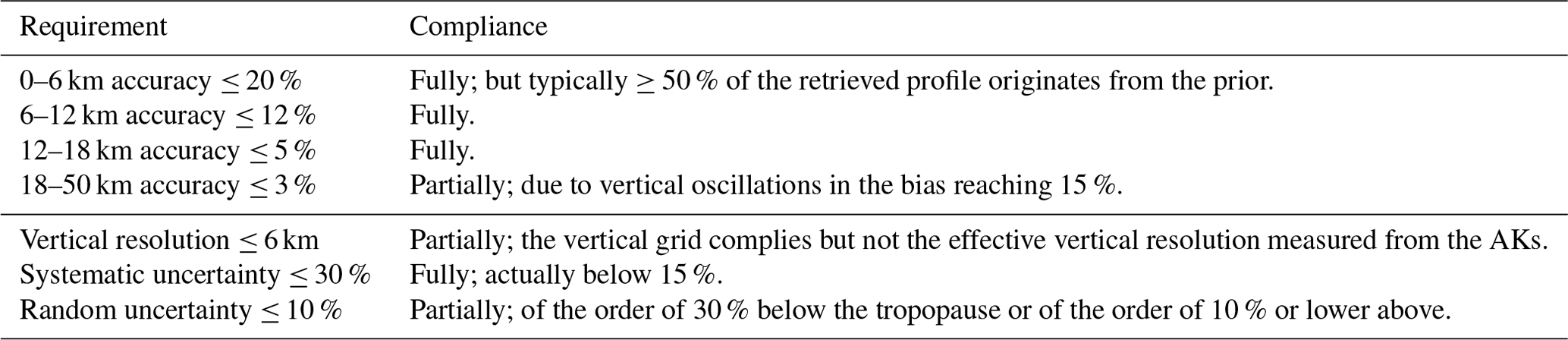
The operational ozone profiles and derived subcolumns are at least partially compliant with all mission requirements. With the accuracy representing the closeness of the satellite observations to the true value as estimated by the reference measurements, the corresponding requirements are on average fully met for the lowest three subcolumns. This can be seen in Fig. 10, with the horizontal thick black lines (average differences that are constant for each row) being within the grey areas (SRD requirements). Due to vertical bias oscillations, however, reaching up to about 15 %, the subcolumns above 24 km do not always comply with the accuracy requirement of 3 % above 18 km.

The requirements for the bias are less strict (in terms of systematic uncertainty in the comparisons) for the entire profile in the GVR. The vertical bias oscillations in the stratosphere reaching up to 15 % are still much below the 30 % limit. On the other hand, the random uncertainty requirement is only met above the UTLS. Around the UTLS and in the troposphere, the comparison dispersion reaches 30 % and hence does not comply. The vertical resolution only partially complies with the GVR too. The vertical retrieval grid is sampled at a resolution of 6 km or higher, but the effective vertical resolution of the profile equals 10 to 15 km on average and goes down to 7 km at minimum, thus just not meeting the resolution requirement.

4.7 Mutual consistency with other TROPOMI ozone products

A straightforward check that is also performed on a daily basis from the TROPOMI level 2 quality portal is verifying whether the integrated ozone profile matches the total ozone column retrieval. The integrated ozone column from the subcolumns of the ozone profile product is compared with the vertical column of the TROPOMI GODFIT Total Ozone product (Garane et al., 2019) in Fig. 13. It shows that the relative difference between the two columns in the month of October 2020 (RPRO datasets) typically amounts to about 5 %, meaning that the integrated profile slightly underestimates the total column retrieval, although geographical features seem to be well captured, as seen for the six subcolumns in Fig. 5. A slightly higher bias can be observed in the Atlantic Ocean west of Southern Africa, which might be due to the difference in the climatology implementation between the two products. This is under investigation and will be discussed in a follow-up paper. Taking into account possible drifts described above, this makes the operational TROPOMI ozone profile product and its (sub)column derivatives suitable for studies of atmospheric chemistry and dynamics but not for vertically resolved trend studies.

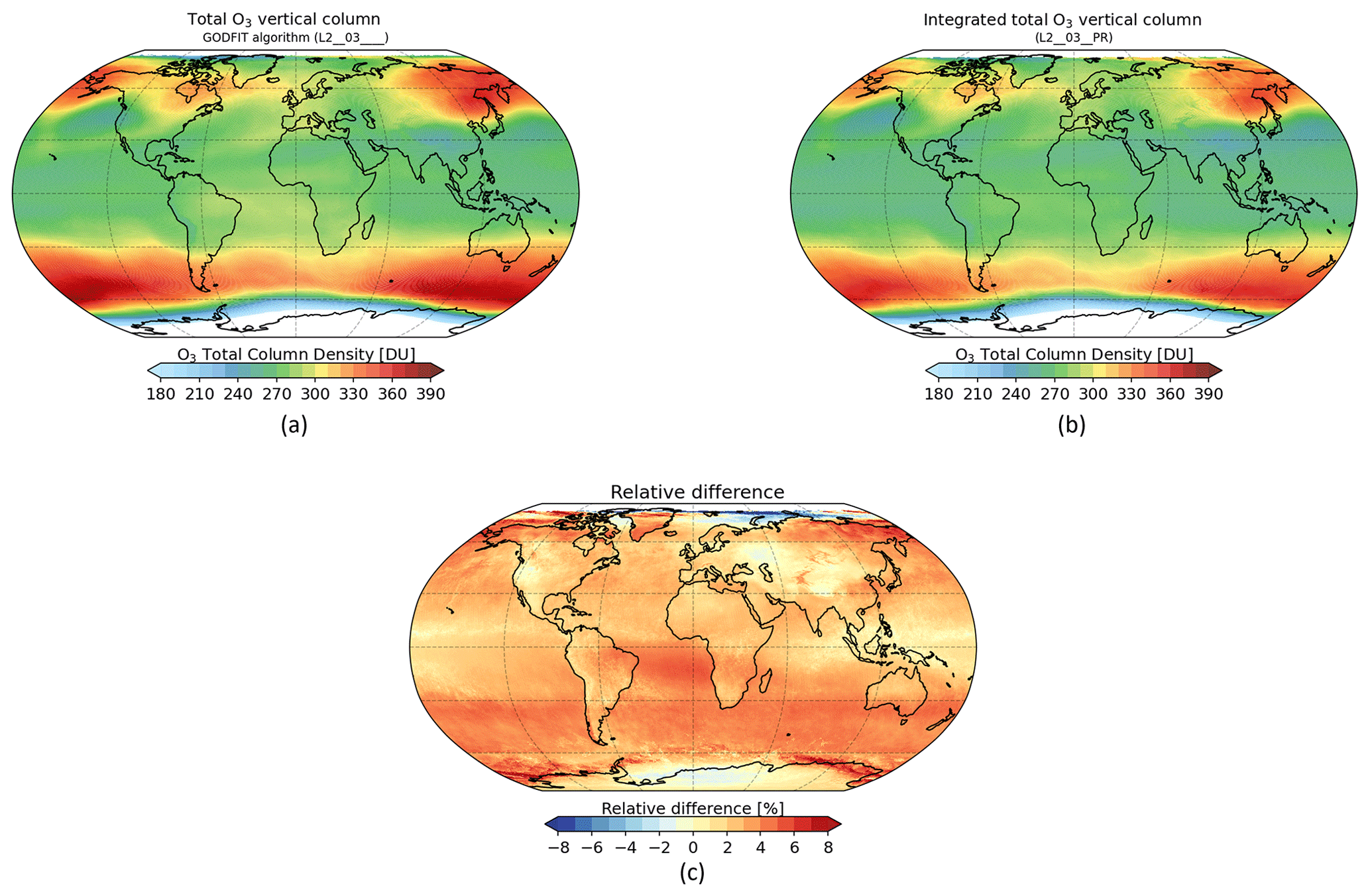
Figure 13 The October 2020 total ozone column average of the operational TROPOMI GODFIT algorithm (L2__O3____) in panel (a) and the integrated operational ozone profile product in panel (b). Panel (c) shows their relative difference.

The operational TROPOMI ozone profile validation results obtained in this work are additionally compared with those of the scientific TROPOMI ozone profile retrieval algorithms that have been found in the literature (see the Introduction). However, as the validation approaches for these products are not matched, this comparison should be considered with caution and within their spatiotemporal validity. Zhao et al. (2020) selected five stations globally to compare their TROPOMI product, based on the operational L1B v1.0, with ozonesonde profiles from March 2018 to December 2019. Their TROPOMI retrieval agreed with the ozonesondes to within ±5 % from 0.8–30 hPa and within ±15 % below 30 hPa, thus performing comparably to the operational retrieval around the UTLS while somewhat worse below. Their TROPOMI retrievals showed a significant reduction in mean biases over the climatological profiles below 30 hPa, while the retrieved ozone profiles showed worse agreement with ozonesondes than the a priori profile above 20 hPa, mainly due to not using measurement information below 314 nm.

The TOPAS ozone profile retrieval, already based on L1B v2.0, was validated by comparison with ozonesonde and stratospheric lidar data between June 2018 and October 2019 (Mettig et al., 2021). The validation with lidar measurements showed a bias within ±5 % between 15 and 45 km, with a standard deviation of 10 %, thus doing slightly better than the operational algorithm. The validation with ozonesondes showed comparable agreement in the lower stratosphere, with deviations of less than ±5 % at all latitudes in the altitude range 18–30 km and a standard deviation of the mean differences of about 10 %. Below 18 km, on the other hand, the relative mean deviation in the tropics and northern latitudes remained within ±20 %. At southern latitudes, larger differences of up to +40 % occurred between 10 and 15 km. The standard deviation is about 50 % between 7 and 18 km and about 25 % below 7 km. The combined TROPOMI-CrIS TOPAS retrieval showed reduced mean differences and standard deviations with respect to tropospheric lidar data (limited to the northern subtropical region) in comparison to the UV-only retrieval (Mettig et al., 2022). The validation with ozonesondes showed rather minor improvements.

The MUSES algorithm was used for CrIS-TROPOMI, CrIS-only, and TROPOMI-only ozone profile retrievals from September 2019 to August 2020 (Malina et al., 2022). The TROPOMI-only precision was typically below 5 % in the troposphere, in agreement with the operational retrieval results. CrIS-only showed a mean bias between 1.4 % and 10.4 %, depending on the season. The performance of the joint retrieval was comparable to that of CrIS-only, with evidence that the joint retrieval provided benefit over CrIS-only with mean biases between 0.2 % and 7.4 %. All three products showed comparable root mean square errors in the tropospheric difference of about 20 % or below, which is typically somewhat lower than for the operational TROPOMI product.

5 Conclusions

This work reports on the operational retrieval and geophysical validation of Sentinel-5P TROPOMI nadir ozone profile data carried out by the ESA/Copernicus Atmospheric Mission Performance Cluster (ATM-MPC). The NL-L2 processor version 2.4.0/2.5.0 was developed at KNMI and derives ozone number densities at 33 pressure levels from the TROPOMI reflectance observations provided by bands 1 and 2 of the UV detector, using L1B processor v2. The main elements of the operational retrieval algorithm include several pre-processing steps, the forward model, and the optimal estimation based on the inverse model. Despite the TROPOMI pixel resolution increase in August 2019 and the soft-calibration changes in July 2022 and January 2023 reducing along-orbit striping, a consistent 5-year ozone profile record, spanning May 2018 to April 2023, is obtained for the entire sunlit Earth.

The comprehensive quality assessment of the TROPOMI ozone profile data record combines results from both the ATM-MPC Validation Data Analysis Facility and the S5P Validation Team. The prescribed validation methodology includes the analysis of satellite data content, retrieval information diagnostics, and comparisons with co-located ground-based reference measurements. The latter are acquired by ozonesondes contributing to WMO's Global Atmosphere Watch, by tropospheric lidars from the Tropospheric Ozone Lidar Network, and by NDACC stratospheric lidars. By the application of tight co-location criteria (same-day overpasses) and averaging kernel smoothing of the reference observations, sampling and smoothing difference errors are reduced to a minimum. Comparison of the TROPOMI ozone profile data with the reference observations then concludes to a median agreement better than 5 to 10 % in the troposphere. The median bias goes up to −15 % in the upper stratosphere, exhibiting vertical oscillations. The comparisons show a dispersion of about 30 % in the troposphere and 10 %–20 % above. Chi-square tests on these uncertainties demonstrate that the observed differences confirm the satellite (and ground) uncertainty estimates in the stratosphere. Around the tropopause and below, the total TROPOMI uncertainty is on average underestimated by a factor of 2 at maximum.

The information content of the operational TROPOMI ozone profile retrieval is assessed through the analysis of its averaging kernels. Although each ozone profile is characterised by about five to six independent pieces of information (DFS), it must be kept in mind that these are not equally distributed over the derived product consisting of six subcolumns. The kernel matrix row sums reveal a vertical sensitivity close to 100 % at all altitudes from about 20 to 50 km yet decrease rapidly above and below. Towards the surface, on average 50 % of the retrieved information originates from the prior profile. The corresponding kernel peaks at about 10 km altitude on average. Typically, the kernel peak (information barycentre) only lies at the nominal retrieval altitude where the sensitivity approaches unity. As another measure of the vertical sounding accuracy, the effective vertical resolution of the profile retrieval usually ranges within 10–15 km, with a minimum close to 7 km in the middle stratosphere, which is below the retrieval grid resolution (6 km at maximum). The higher sensitivities and effective vertical resolutions are typically observed for longer atmospheric optical paths, i.e. for solar zenith angles above 60 °.

The path length dependence of the retrieval information content also translates into seasonal and meridian dependencies of the – especially tropospheric – bias and affects the oscillations in the stratospheric bias. A similar but reduced effect can be seen for the viewing zenith angle. Additionally, the bias is negatively correlated with the surface albedo for the lowest subcolumns, despite the albedo's apparently slightly positive correlation with the retrieval degrees of freedom. For the lowest retrieval levels (0–6 km), this correlation looks as if it is somewhat compensated by the increased atmospheric penetration of the sunlight at low solar zenith angles (0–30 °). On the other hand, one can also observe lower-DFS profiles with near-zero surface sensitivity in combination with a highly overcompensating sensitivity around the UTLS ranging up to three and above. These retrievals occur for scenes that have both high SZA and high surface albedo, mostly around the Antarctic.

The 5 years of TROPOMI ozone profile data under study show a slight DFS degradation throughout the mission (next to a jump from the ground pixel resolution change). Comparisons with the ozonesonde data reveal significant positive drifts near 2 % yr⁻¹ in the tropics and mid-latitudes from the surface to the UTLS, while 1 % yr⁻¹–2 % yr⁻¹ negative drifts are observed for the stratospheric ozone retrievals. This makes the current operational TROPOMI ozone profile product and its subcolumn derivatives unsuitable for vertically resolved trend studies. However, no significant drift is detected for the vertically integrated profile. This agrees with the operational TROPOMI total ozone column retrieval (Garane et al., 2019), although the latter is consistently about 5 % higher than the integrated ozone profile.

Four scientific TROPOMI ozone profile retrieval algorithms have been described in the literature. Two of these also provide joint retrievals with the infrared CrIS instrument that orbits 3 min ahead of S5P. Bremen University's TOPAS product performs slightly better (showing a vertically consistent 5 % bias) than the operational one in the stratosphere, while NASA's MUSES algorithm shows total tropospheric uncertainties below 20 %. Apart from these exceptions, the operational ozone profile product demonstrates a comparable or lower uncertainty than the scientific products. It is moreover found to be at least partially compliant with all mission requirements. The TROPOMI instrument as such provides a crucial component to the present-day global ozone observing system. It provides important contributions to, amongst others, the Global Climate Observing System (GCOS), ESA's Climate Change Initiative on ozone (and its Climate Space follow-up), the Copernicus Climate Change Service (C3S), the International Global Atmospheric Chemistry (IGAC) Tropospheric Ozone Assessment Report Phase II (TOAR-II), and several activities endorsed by the Committee on Earth Observation Satellites (CEOS).