the Creative Commons Attribution 4.0 License.
the Creative Commons Attribution 4.0 License.
 | 15 Jul 2024
The algorithm of microphysical-parameter profiles of aerosol and small cloud droplets based on the dual-wavelength lidar data
Huige Di
Xinhong Wang
Ning Chen
Jing Guo
Wenhui Xin
Shichun Li
Yan Guo
Qing Yan
Yufeng Wang
Dengxin Hua
This study proposed an inversion method for atmospheric-aerosol or cloud microphysical parameters based on dual-wavelength lidar data. The matching characteristics between aerosol and cloud particle size distributions and gamma distributions were studied using aircraft observation data. The feasibility of the retrieval of the particle effective radius from lidar ratios and backscatter ratios was simulated and studied. A method for inverting the effective radius and number concentration of atmospheric aerosols or small cloud droplets using the backscatter ratio was proposed, and the error sources and applicability of the algorithm were analyzed. This algorithm was suitable for the inversion of uniformly mixed and single-property aerosol layers or small cloud droplets. Compared with the previous study, this algorithm could quickly obtain the microphysical parameters of atmospheric particles and has good robustness. For aerosol particles, the inversion range that this algorithm can achieve is 0.3–1.7 µm. For cloud droplets, it is 1.0–10 µm. An atmospheric-observation experiment was conducted using the multi-wavelength lidar developed by Xi'an University of Technology, and a thin cloud layer was captured. The microphysical parameters of aerosol and clouds during this process were retrieved. The results clearly demonstrate the growth of the effective radius and number concentration.
- Article
(5891 KB) - Full-text XML
- BibTeX
- EndNote


The vertical characteristics of aerosol and clouds are of great significance for the study of many scientific issues, such as the interaction between aerosol and clouds, the mechanism of atmospheric pollution generation, and so on (Lohmann and Feichter, 2005; Kulmala et al., 2004; Miffre et al., 2010). The high-precision detection of aerosol and cloud microphysical parameters at vertical altitudes is important. At present, the main methods for obtaining atmospheric-aerosol or cloud microphysical parameters include in situ observation (He et al., 2019; Moore et al., 2021; Gao et al., 2022a, b) and remote sensing observation (Vivekanandan et al., 2020; Johnson et al., 2009). People can obtain microphysical parameters of clouds or aerosol at vertical altitudes by mounting in situ observation instruments on equipment such as airplanes or balloons (Kaufman et al., 1998; Cai et al., 2022), but this method has a low detection frequency and cannot obtain continuous observation data with high temporal and spatial resolutions (Zhao et al., 2018). Lidar, with its advantages of high temporal and spatial resolutions and a high detection sensitivity, has been widely used in the field of atmospheric detection and has important application potential in detecting the optical and microphysical parameters of atmospheric aerosol and clouds (Vivekanandan et al., 2020; Hara et al., 2018; Siomos et al., 2017; Kanitz et al., 2013; Dionisi et al., 2018).
The remote sensing detection of aerosol microphysical parameters mainly uses three-wavelength lidar, which can obtain four or more optical parameters (usually requiring two extinction coefficients at 355 and 532 nm and three backscatter coefficients at 355, 532, and 1064 nm) for the retrieval of aerosol microphysical parameters (Veselovskii et al., 2004; Müller et al., 1999; Veselovskii et al., 2009). The regularization algorithm (Kolgotin et al., 2023; Veselovskii et al., 2002), the principal component analysis (PCA) technique (de Graaf et al., 2013), and the linear estimation algorithm (Veselovskii et al., 2012) have been used for determining the aerosol bulk properties. These algorithms do not require the assumption of a complex refractive index or aerosol particle size distribution (APSD); thus, they have been widely studied, but their applications are limited. The inversion results are unstable, and there will be good results under certain spectral types; however, in some cases, the inversion error is very large. In addition to this, the above methods require complex lidar hardware systems (Di et al., 2018a; Meskhidze et al., 2021; Müller et al., 2014). Therefore, the above algorithms cannot be applied well in most lidar systems (most lidars in AERONET are dual-wavelength), and it is necessary to establish a more reasonable method for inverting microphysical parameters. For clouds, there are two methods used for the detection of cloud microphysical parameters. The first method is using lidar–radar synergy for cloud microphysical parameters (Wang and Sassen, 2002; Vivekanandan et al., 2020; Zhang et al., 2021), which can achieve the retrieval of cloud droplets with large cloud particles. For thin and sparse clouds or nascent clouds, cloud droplet particles are usually small and cannot be detected by millimeter-wave cloud radar, which affects the application of this method. The second method is to use multiple scattering information in clouds detected by multi-field-of-view (FOV) or dual-FOV lidar to retrieve the microphysical parameters of water clouds (Wang et al., 2022). However, in order to obtain multiple scattering signals using ground-based lidar, the larger FOV of a telescope is required, which will greatly affect daytime detection.
This study proposes an inversion method for atmospheric-aerosol or cloud microphysical parameters based on dual-wavelength lidar. This article includes the following parts: in Sect. 2, we study the APSD and cloud droplet size distribution (CDSD) measured by airborne instruments and find that they are basically consistent with the gamma distribution, and we extract the statistical characteristics of the gamma distribution parameters. In Sect. 3, the inversion method and simulation analysis results are presented and described. In Sect. 4, an atmospheric-observation result obtained using lidar is presented. Sect. 5 presents the conclusions and a discussion.
2.1 Gamma distribution
The particle size distribution (Di et al., 2018a) is the variation in particle number with particle radius within a certain radius range (r ∼ r+ dr) per unit volume, defined as
Here, r is the particle radius, n(r) is the particle size distribution, and N is the total number of particles per unit volume. The effective radius (Di et al., 2018a) is an important parameter that characterizes the average particle size, defined as the ratio of the third-order and second-order moments of the particle size distribution, as shown below:
The most common models for APSD are the Junge distribution and lognormal distribution. CDSD is usually described as the gamma distribution or the corrected gamma distribution (Kolgotin et al., 2023). The gamma function has the advantages of integrability and recursion of various order functions. In this paper, the gamma distribution is used to describe APSD and CDSD and is shown as
Here, a is related to particle concentration; b is a dimensionless parameter representing shape factor, which is related to spectral width; and c is a slope parameter.
In mathematics, Γ(x) is defined as the gamma function and is as shown follows:
Its pth moment of the gamma distribution can be expressed as
The effective radius requires second-order and third-order moments, which are shown as follows:
Substituting Eqs. (6) and (7) into Eq. (2) yields the effective radius as follows:
The gamma function has recursion, as shown in the following formula:
According to Eqs. (8) and (9), the effective radius can be simplified as
2.2 APSDs and CDSDs in the vertical altitude
In order to study the characteristics of APSDs and CDSDs in the vertical altitude, the APSDs and CDSDs obtained from aircraft observations by the Hebei Provincial Weather Modification Office were analyzed (from 2005 to 2006). APSDs were measured by the PCASP-100X probe, and CDSDs were obtained by the FSSP-100-ER probe (Di et al., 2018b). The PCASP-100X is an optical particle counter for measuring aerosol size distributions from 0.10 to 3.00 µm in diameter in 15 different size bins at a frequency of 1 Hz. The sample flow volume in the PCASP-100X was set to 1 cm3 s−1. FSSP-100-ER is an instrument that measures cloud droplet size and concentration using light scattering, with the measurement range of 0.5–47 µm.
The obtained APSDs and CDSDs were fitted one by one using the gamma function, and we statistically analyze these fitting parameters. In order to minimize the error for all radii, the minimization problem is solved using the following equation:
Here, fm(D) is the actual particle size distribution measured by the PCASP-100X, ffitted(D) is the fitted distribution, D is the aerosol particle diameter, and Dmax is the measured maximum particle diameter. The goodness of fit R2 is used to represent the difference between the fitting function and the measured data. The definition of goodness of fit is as follows:
where yi is the measured value, is the predictive value, and is the mean measured value. The numerator represents the sum of squared residuals, and the denominator represents the sum of squared total deviations.
Approximately 3500 sets of APSDs and 2221 sets of CDSDs were statistically analyzed. Over 95 % of the data have a high goodness of fit in the gamma distribution. The goodness of fit of CDSDs is higher than that of APSDs, with CDSDs showing a goodness of fit of 0.983 and APSDs showing a goodness of fit of 0.856. The parameter a of CDSDs is significantly larger than that of APSDs, and there are obvious differences between b and c for clouds and aerosol. The literature suggests that there is a certain functional relationship between the gamma parameters b and c of CDSDs (Ding et al., 2023). Statistical analysis was conducted on the b and c parameters of APSDs and CDSDs, as shown in Fig. 1.
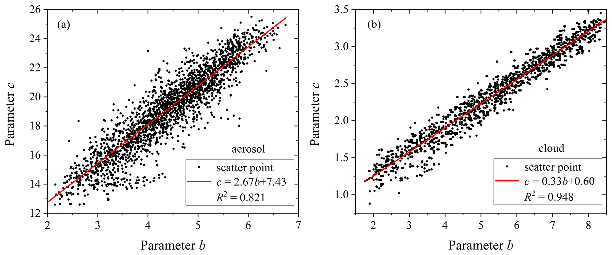
Figure 1Statistical results of parameter b and c in aerial survey data. (a) Aerosol particles. (b) Cloud droplets.
According to Fig. 1, there are remarkable linear relationships between parameters b and c. The fitting functions for CDSDs and APSDs are as follows:
The linear relationship between the two parameters of CDSDs is better, with a goodness of fit of 0.948 compared to the linear goodness of fit of 0.821 for APSDs. According to the statistical results, the parameter b of APSDs at vertical heights is mainly distributed in the range of 2–7, and that of CDSDs is mainly distributed in the range of 2–8.
3.1 Inversion algorithm
The first step in this algorithm is the retrieval of the effective radius. The parameter a in the gamma distribution shown in Eq. (4) is related to the number concentration. The ratio OR(m,r) (lidar ratio or color ratio) of the two optical parameters can eliminate parameter a and can be written as
Here, m is the complex refractive index of particles, and g1(λ1) and g2(λ2) are the optical parameters at the two wavelengths λ1 and λ2, respectively. The ratio can also be written as follows:
where Q1 and Q2 are the extinction efficiency factors or backscattering efficiency factors at λ1 and λ2. Using the effective radius in Eq. (10) instead of parameter c, Eq. (13) can be written as follows:
According to Eqs. (11) and (14), if the ratio of optical parameters monotonically changes with the effective radius, the effective radius can be obtained from the ratio of optical parameters, and then parameters b and c can also be obtained according to Eq. (11). The ratio here can be chosen as the ratio of the backscatter or extinction coefficients of two wavelengths (color ratio) or the ratio of the extinction coefficient of one wavelength to the backscatter coefficient (lidar ratio).
After obtaining b and c, a can be derived from Eq. (15), written as
Then, the number concentration N can be calculated by integrating Eq. (4). The algorithm flowchart is shown below.

The algorithm is described below.
In this algorithm, the first step is to establish a lookup table between aerosol and cloud optical parameters and microphysical parameters. (1) Assuming that aerosol particles and cloud droplets follow the gamma distributions, we calculate the extinction coefficient and backscatter coefficient at different laser wavelengths (355 and 1064 nm in this paper) based on the Mie scattering theory. (2) We calculate the ratio of backscatter coefficients for two wavelengths, which is the backscatter color ratio, or we calculate the ratio of the extinction coefficient to the backscatter coefficient, which is the radar ratio. (3) We change the parameters of the aerosol to obtain the gamma distributions with an effective radius from 0.2 to 3 µm, calculate the optical parameters and corresponding optical parameter ratios (radar ratio or backscatter color ratio) for each gamma distribution, and establish the lookup table for the aerosol effective radius. (4) Similarly to step 3, we establish the lookup table for cloud drops (effective radii are from 0.5 to 5 µm). After the lookup table is completed, the microphysical parameters of aerosols or clouds are calculated based on the lookup tables and lidar detection data. The specific steps are as follows: (1) the dual-wavelength (355 and 1064 nm) Raman lidar need be selected for the detection of the atmosphere; (2) the Raman and Fernald methods are used for the retrieval of optical parameters at multiple wavelengths, and the backscatter color ratio or lidar ratio can be obtained; (3) aerosol and cloud layers are identified based on lidar echo signals; (4) we retrieve the effective radius of aerosol or cloud droplets at different heights based on optical parameter ratios and lookup tables; (5) we calculate the parameters b and c in the gamma distribution according to Eqs. (13) and (16); (6) we calculate the value of a in the gamma distribution according to Eq. (17); and (7) we calculate the number concentration according to Eq. (3).
3.2 The simulation
3.2.1 The relationship between lidar ratio, color ratio, and effective radius
Due to the different complex refractive indices of aerosols and clouds, we will discuss these separately. Water clouds are composed of liquid droplets, and so the complex refractive index of 1.33-10−7i was selected. The theoretical relationship curves of a lidar ratio of 355 nm, a lidar ratio of 532 nm, a backscatter color ratio of 355 nm 1064 nm, and a backscatter color ratio of 355 nm 532 nm with an effective radius were calculated and are shown in Fig. 3a to d.

Figure 3The theoretical relationship curves of color ratios or lidar ratios with an effective radius (m=1.330.10−7i). (a) Lidar ratio of 355 nm, (b) lidar ratio of 532 nm, (c) the ratio of backscatter coefficients (355 nm 1064 nm), and (d) the ratio of backscatter coefficients (355 nm 532 nm).
The composition of aerosol is complex, with a large variation in the complex refractive index, ranging from 1.33 to 1.70 in the real part and from 0 to 0.05 in the imaginary part. Assuming the complex refractive index of aerosol is 1.47-0.002i, Fig. 4a to d, respectively, show the theoretical relationship curves of aerosol when parameter b is set to 2–7.

Figure 4The theoretical relationship curves of color ratios or lidar ratios with an effective radius (m= 1.470.002i). (a) Lidar ratio of 355 nm, (b) lidar ratio of 532 nm, (c) the ratio of backscatter coefficients (355 nm 1064 nm), and (d) the ratio of backscatter coefficients (355 nm 532 nm).
The blue boxes in Figs. 3 and 4 refer to the monotonic variation intervals of aerosol and cloud droplets, respectively. As shown in the figures, when the complex refractive index is constant and the parameter b is set to 2–7 or 2–8, the corresponding curve trend is consistent. Under a constant complex refractive index, parameter b does not change the trend of the curve. The change in b has little effect on the curve. If the color ratio (355 nm 1064 nm) is selected for the retrieval of the effective radius, the influence of the value of b on the results is about 5 % (as shown in Figs. 3c and 4c). If the lidar ratio is selected for the retrieval of the effective radius, the influence of the value of b on the results will be slightly greater, and it might reach ∼ 10 % (as shown in Figs. 3a and 4a). Within the monotonic interval, the effective radius of particles can be retrieved from the curves. The monotonic interval varies with optical parameter. It can be seen that, whether it is clouds or aerosol, the monotonic range of the backscatter color ratio is the widest, as shown in Figs. 3c and 4c. The larger the value of b, the more pronouncedly the gamma function describes the characteristics of large particles. Therefore, in the subsequent inversion, b = 6 is taken for cloud droplets, and b = 3 is taken for aerosol.
Considering the laser's penetration ability, along with the monotonic range of optical parameter ratios with an effective radius shown in Figs. 3 and 4, the backscatter ratio of 355 nm 1064 nm for the inversion is the optimal choice. According to Fig. 3c, the effective radius that can be retrieved using the backscatter ratio of 355 nm 1064 nm is above 1 µm. The optimal inversion range is 1–3.4 µm, and the maximum inversion radius can reach 10 µm. For aerosol particles, the theoretical retrieval effective radius is above 0.3 µm, and the optimal inversion interval is 0.3–1.7 µm. The applicability of this algorithm is limited, and it is applicable for aerosol and small cloud droplets. For aerosol, particle diameter is usually 0.01 to 10 µm, while the effective particle radius ranges from 0.3 to 1.2 µm for urban aerosol. This is calculated based on ground and aircraft observation data. Usually, water droplets with diameters larger than 2 µm are called cloud droplets. Therefore, this algorithm is suitable for the detection of urban aerosol and small cloud drops. The above curves in Figs. 3 and 4 are calculated using Mie scattering theory and are suitable for spherical particles. The spherical particles in the atmosphere can be distinguished from the depolarization ratio.
3.2.2 The influence of complex refractive index on the backscatter color ratio
When the complex refractive index changes and b is 3, the backscatter color ratios of the 355 and 1064 nm wavelengths are shown in Fig. 5a to d.
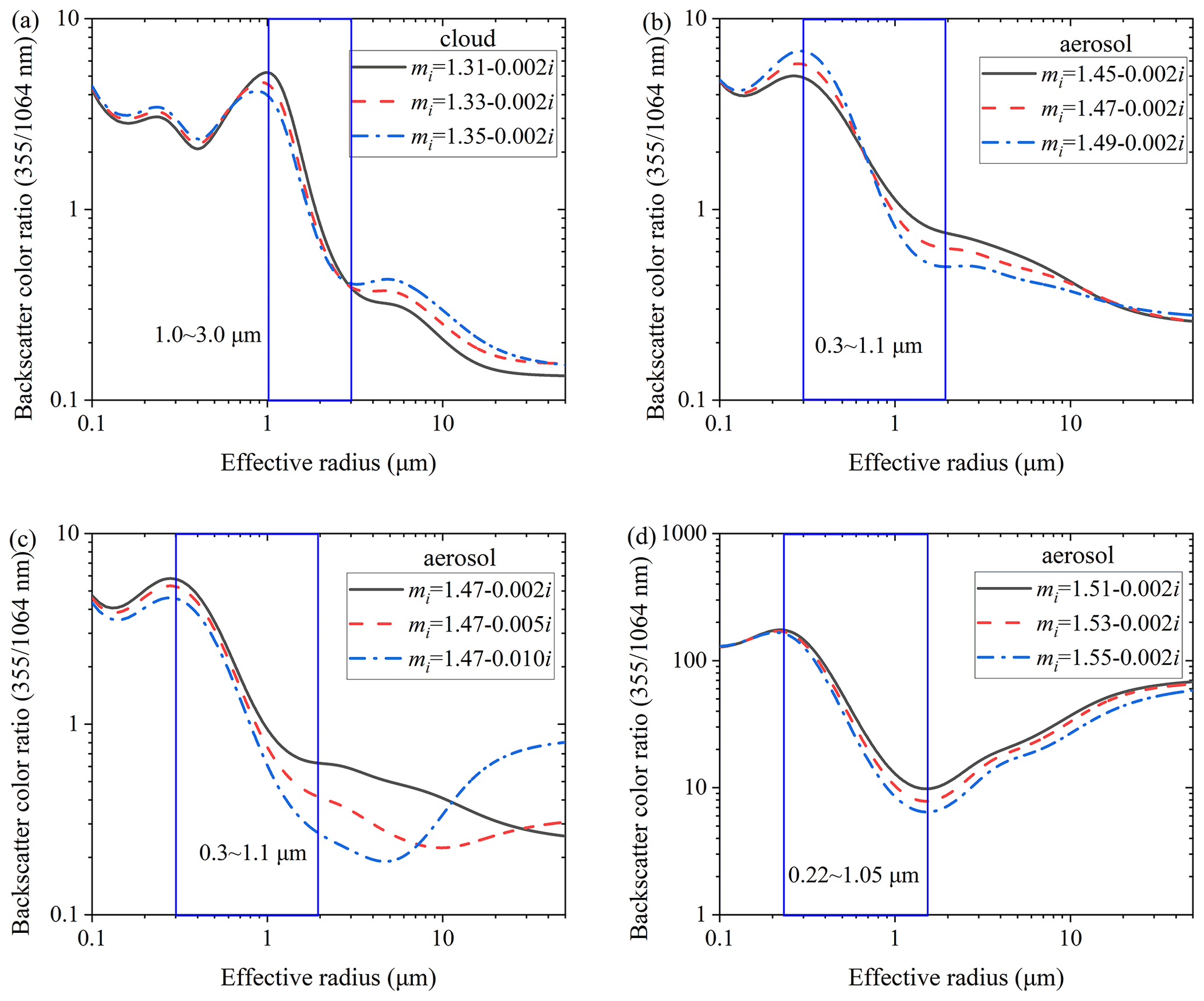
Figure 5The color ratio with different complex refractive indices. (a) Aerosol with different real parts of the complex refractive index (real part < 1.50), (b) aerosol with different imaginary parts of the complex refractive index (real part < 1.50), (c) aerosol with different real parts of the complex refractive index (real part > 1.50), and (d) aerosol with different imaginary parts of the complex refractive index (real part > 1.50).
According to Fig. 5, when the complex refractive index of particles changes, the color ratio curves will fluctuate, but they always monotonically decreases from 0.3 to 1 µm. Therefore, if the aerosol composition is stable, the color ratio curve can well reflect the trend of effective radius variation.
3.2.3 Algorithm verification
The verification of this algorithm is achieved through simulation. The specific steps are as follows: (1) calculate the effective radius and number concentration using APSD and CDSD observed by aircraft and Eq. (8); (2) calculate the backscatter coefficient at two wavelengths of 355 and 1064 nm, and then calculate the color ratio according to Eq. (13); (3) according to the color ratio and the algorithm described in Fig. 2 of Sect. 3.1, the effective radius and number concentration profiles can be retrieved; and (4) compare the effective radius and numerical concentration in steps 2 and 4, as shown in Fig. 6, to verify the algorithm inversion.
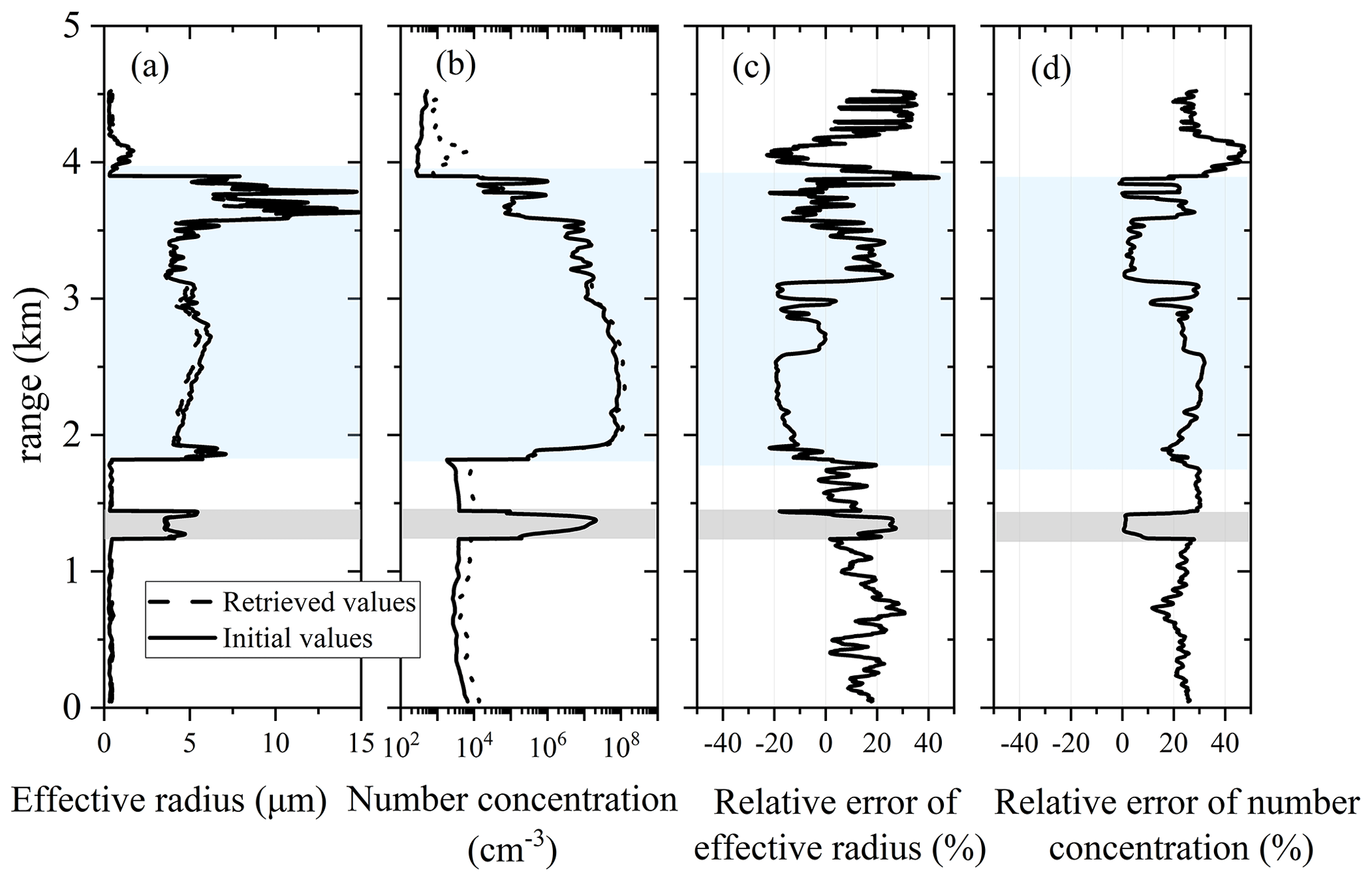
Figure 6Simulation and verification of the algorithm with aircraft data. (a) Effective radius, (b) number concentration, (c) effective radius error, (d) number concentration error.
Figure 6a and b are the true values and inversion results of the effective radius and number concentration, respectively, of an aircraft observation at vertical altitude. Figure 6c and d show the relative errors, respectively. The light-gray- and light-blue-shaded areas in the figures are cloud layers. It can be seen that the effective radius and number concentration can be retrieved well using the algorithm. Figure 6 shows that the retrieval error of cloud droplets is relatively small, within ±20 % and ±30 % for the effective radius and number concentration. The errors are ±20 % and ±40 % for aerosol. The inversion error of the microphysical parameters of aerosol particles is larger than that of cloud droplets. The reasons are that (1) aerosol types are more complex, and the assumption of a complex refractive index is prone to deviation, and (2) APSDs are more complex than CDSDs, and the adaptability to the gamma distribution is relatively low.
3.3 Error analysis of the algorithm
The inversion errors of the effective radius and number concentration mainly come from three aspects: (1) error introduced by non-spherical particles, (2) error introduced by the assumption of a gamma distribution, (3) error introduced by improper assumption of a complex refractive index, and (4) error caused by optical parameter inversion deviation.
For urban aerosol and water clouds, the particles are spherical; thus, the error caused by non-spherical particles can be ignored. The error introduced by the assumption of a gamma distribution is relatively complex and difficult to accurately calculate. This study evaluates this error by means of numerical simulation based on APSD and CDSD data obtained by aircraft observations. Actually, the error presented in Fig. 6 is mainly caused by the assumption of a gamma distribution. We calculate the optical parameters of over 5000 sets of APSD and CDSD data, and we retrieve the microphysical parameters using our algorithm. The calculated standard deviations between the inversion results and the actual data are as follows: for aerosols, the standard deviation of the effective radius is ∼ 10 %, and the standard deviation of the numerical concentration is ∼ 20 %; for clouds, the standard deviation of the effective radius is 15 %, and the standard deviation of the numerical concentration is ∼ 20 %.
The deviation introduced by the improper assumption of a complex refractive index may be the largest term in this technique. For water clouds, the complex refractive index is stable, and the deviation caused by it can be ignored. It is difficult to accurately obtain the complex refractive index of aerosol, and the deviation caused by the complex refractive index may reach over 100 %. Figure 6 shows the effect of the complex refractive index variation on the optical parameter ratio. From Fig. 6, it can be seen that, when the real part of the complex refractive index changes within the range of 0.03 and when the imaginary part changes within 0.01, the effective radius deviation caused by the complex refractive index is within a controllable range. After calculation, the deviation does not exceed 40 %. Furthermore, it can be seen that, although complex refractive index can lead to a significant change in the effective radius value, when the aerosol is constant, its monotonic characteristics remain unchanged, which means that the evaluation of particle size changes is reliable.
In order to quantitatively analyze the impact of optical parameter errors on the effective radius inversion results, the effective radius errors caused by color ratio error are calculated when the errors of the backscatter color ratio are ±5 % and ±10 %, as shown in Fig. 7.
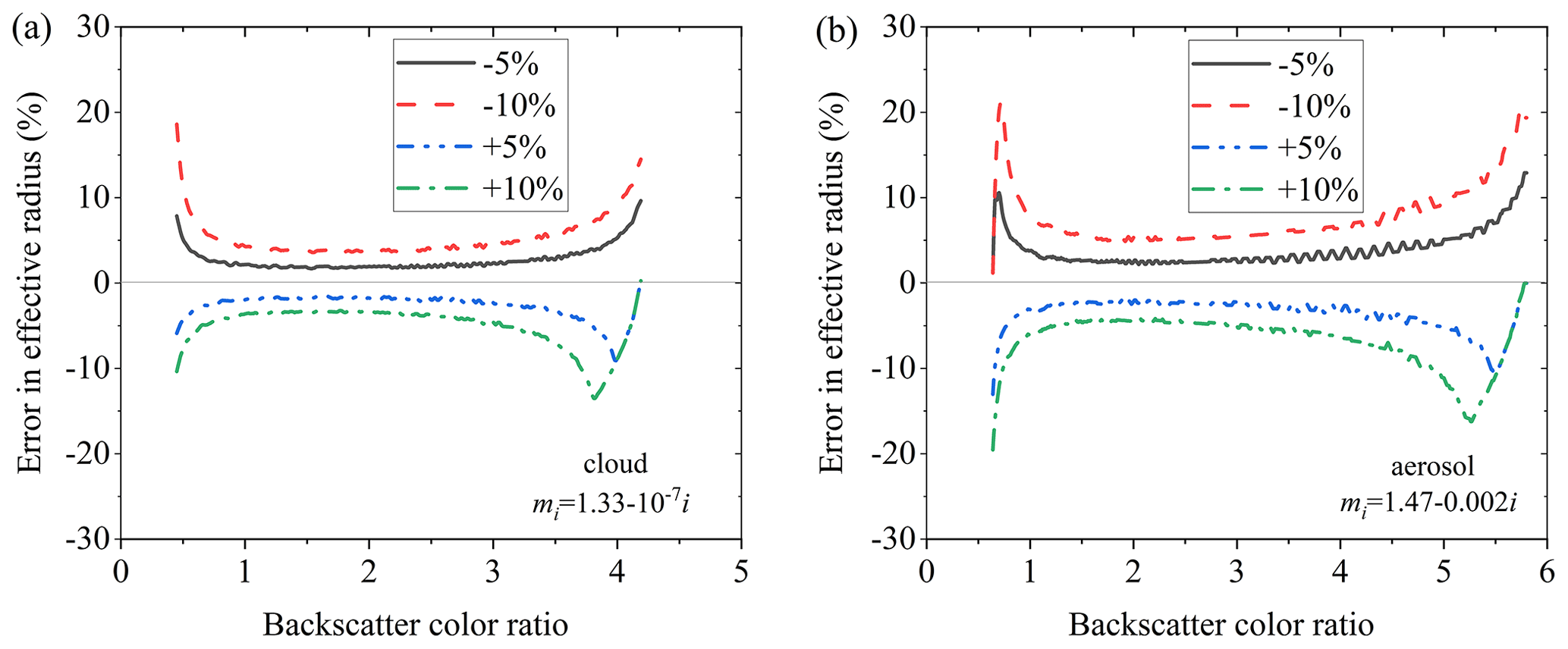
Figure 7Errors in effective radius in lookup table when there are ±5 % and ±10 % errors in the backscatter color ratio. (a) Cloud droplets. (b) Aerosol particles.
From Fig. 7a, it can be seen that, when there are errors of ±5 % and ±10 % in the backscatter color ratio, the inversion errors of the effective radius of cloud droplets are within ±10 % and ±20 %, respectively. According to Fig. 7b, when there are errors of ±5 % and ±10 %, the inversion errors of aerosol effective radius are within ±20 % and ±30 %, respectively.
Considering the actual inversion ability of lidar, the deviation of the color ratio will reach 10 %. The above errors are independent of each other. The final evaluation shows that the mean square deviation of the inversion error of the aerosol effective radius is less than 45 %, and the standard deviation of the inversion error of the cloud droplet effective radius is less than 25 %.
The inversion error of the number concentration comes from the final superposition of the optical parameter error and effective radius error, and the error should be slightly larger than effective radius. In this algorithm, the complex refractive index needs to be assumed. The physical and chemical properties of aerosol particles and cloud droplet particles that interact with the cloud are similar, with a complex refractive index similar to that of the cloud. Continuous microphysical-parameter profiles can be obtained by this algorithm. For the uniformly mixed aerosol layer, it can be considered to be the case that the complex refractive index within the layer remains unchanged. Therefore, this algorithm is suitable for the inversion of microphysical parameters of uniformly mixed aerosol particles and small cloud droplet particles.
4.1 Instrument
A multi-wavelength (355 nm–532 nm–1064 nm) lidar has been developed by the Xi'an University of Technology (XUT). A Cassegrain telescope is employed as the optical receiver, and narrow-band interference filters are utilized as core filter devices to finely separate the backscatter signals. The system consists of five detection channels: the two elastic scattering channels at wavelengths of 355 and 1064 nm, the nitrogen Raman scattering channel at 387 nm, and the two polarization channels at 532 nm. Table 1 summarizes the main system parameters of the lidar system.
Table 1System parameters of multi-wavelength Raman–Mie scattering lidar.

The optical parameters obtained from this system are the backscatter coefficients at 355 nm (β355) and 1064 nm (β1064), the extinction coefficient of 355 nm (α355), and the depolarization ratio of 532 nm (δ532). β355 is obtained by inverting the Mie scattering and Raman channel without assuming a lidar ratio. β1064 can be inverted by the Fernald method, as described in Wang et al. (2023a) and Li et al. (2016).
4.2 The experimental observation of cloud layer
4.2.1 The experimental observation
Experimental observations were performed based on the lidar of XUT at the Jinghe National Basic Meteorological Observing Station (34.43° N, 108.97° E) on 16 September 2022 (BJT). The observation experiment lasted for 7 h, with a temporal resolution of 2 min. Figure 8a shows the time–height intensity (THI) of the Mie–Rayleigh signal at 1064 nm, and the color bar values in the figure are the logarithm of range-square-corrected signal (RSCS). Figure 8b shows the temperature and relative humidity profiles obtained from the sounding balloon at 07:15 CST.
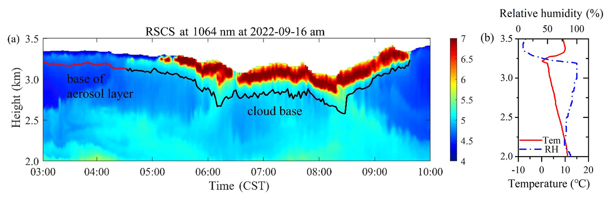
Figure 8Lidar and sounding-balloon observations. (a) THI diagram of RSCS at 1064 nm, observed by lidar at 03:00–10:00 CST on 16 September 2022. (b) Temperature and relative humidity observed by sounding balloon at 07:15 CST on 16 September 2022.
According to Fig. 8a, there are signals changing from weak to strong above the black curve near 3 km. After 05:00 CST, the echo signal gradually increased, and the laser could not penetrate. The red and black lines in the figure correspond to the lower boundaries of the aerosol layer and cloud layer of interest, respectively, calculated by the differential zero-crossing method. According to the temperature and humidity profiles shown in Fig. 8b, the temperature below 3.5 km is higher than 0°, and the relative humidity reaches over 90 % at 3–3.2 km. Therefore, it can be determined that the strong signal appearing near 3 km in the atmosphere is water cloud.
4.2.2 The optical and microphysical-parameter profiles
Figure 9 shows the observed signals of the lidar experiment near 05:00 CST on 16 September 2022, as well as the retrieved optical and microphysical parameters. Figure 9a is the dual-wavelength RSCS with an enhanced signal in the cloud, especially at 1064 nm. Figure 9b shows the volume depolarization ratio profile. The volume depolarization ratio in aerosol and clouds is less than 0.05, indicating that the detected aerosol and clouds are spherical particles. Figure 9c show the dual-wavelength backscattering coefficient profiles at 355 and 1064 nm, while Fig. 9d is the ratio of backscattering coefficients at 355 and 1064 nm, i.e., the backscatter color ratio (Wang et al., 2023b).

Figure 9Lidar observation results at 05:00–05:02 CST on 16 September 2022. (a) Dual-wavelength RSCSs, (b) depolarization ratio, (c) backscatter coefficients, (d) backscatter color ratio, (e) effective radius, and (f) number concentration.
The depolarization ratio of aerosol below the cloud layer does not change significantly, indicating that aerosol are uniformly mixed. Based on the inversion algorithm, the effective radius and number concentration profiles are calculated, as shown in Fig. 9e and f, respectively. In the developing process of clouds shown in Fig. 8, the aerosol hygroscopicity increase plays an important role. According to Fig. 8b, the relative humidity reaches 100 % near 3 km, and below 3 km, the relative humidity is less than 100 %. Therefore, the aerosol lookup table is used below the cloud base for the retrieval of aerosol profiles, and the cloud droplet lookup table is used above the cloud base (gray-shaded area). The effective radius of aerosol under the cloud layer ranges from 1.1 to 1.3 µm, the concentration fluctuates between 17 and 60 cm−3, and the values decrease with increasing height. At the cloud base, the effective radius reaches 1.6 µm, and the concentration is 20 cm−3. As the height above the cloud base increases, the effective radius and number concentration both show an increasing trend. The error bars in Fig. 9 represent the uncertainty of the inversion result. The error of the backscattering coefficient and backscatter color ratio is determined by the signal-to-noise ratio of the lidar system and the error of the optical parameter inversion algorithm. The error bar of the effective radius represents the uncertainty of the results caused by optical parameter errors and gamma distribution assumption errors.
Figure 10 shows the observed signals of the lidar experiment at 07:20 CST on 16 September 2022, as well as the retrieved optical and microphysical parameters. Compared with Fig. 9, the RSCS (Fig. 10a) and backscatter coefficients (Fig. 10c) in the cloud layer increase significantly. From Fig. 10b, it is clear that the depolarization ratio increases above 3.2 km, and this should be caused by multiple scatterings or low signal-to-noise ratios. The effective radius and the numerical concentration of aerosols under the clouds in Fig. 10 show little change compared to Fig. 9. The number concentration in the clouds shown in Fig. 10f has significantly increased, reaching ∼ 2000 cm−3, but the effective radius did not change obviously (only by about 1–2 µm); see Fig. 10e. According to Fig. 8b, it can also be observed that there is a significant inversion layer at 3.2 km; thus, it is normal for there to be more aerosol accumulation below the inversion layer.
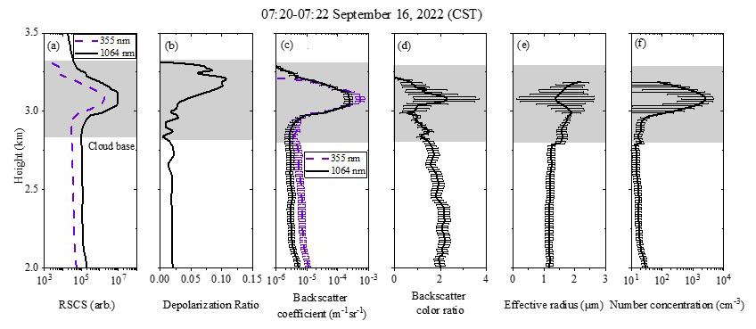
Figure 10Lidar observation results at 07:20–07:22 CST on 16 September 2022. (a) Dual-wavelength RSCSs, (b) depolarization ratio, (c) backscatter coefficients, (d) backscatter color ratio, (e) effective radius, and (f) number concentration.
4.3 The observation results of cloud process
Figure 11 shows the THI of the color ratio. In the region with cloud, the color ratio is relatively small (about 0.5–2), and the color ratio of aerosol is relatively large (about 2–7).
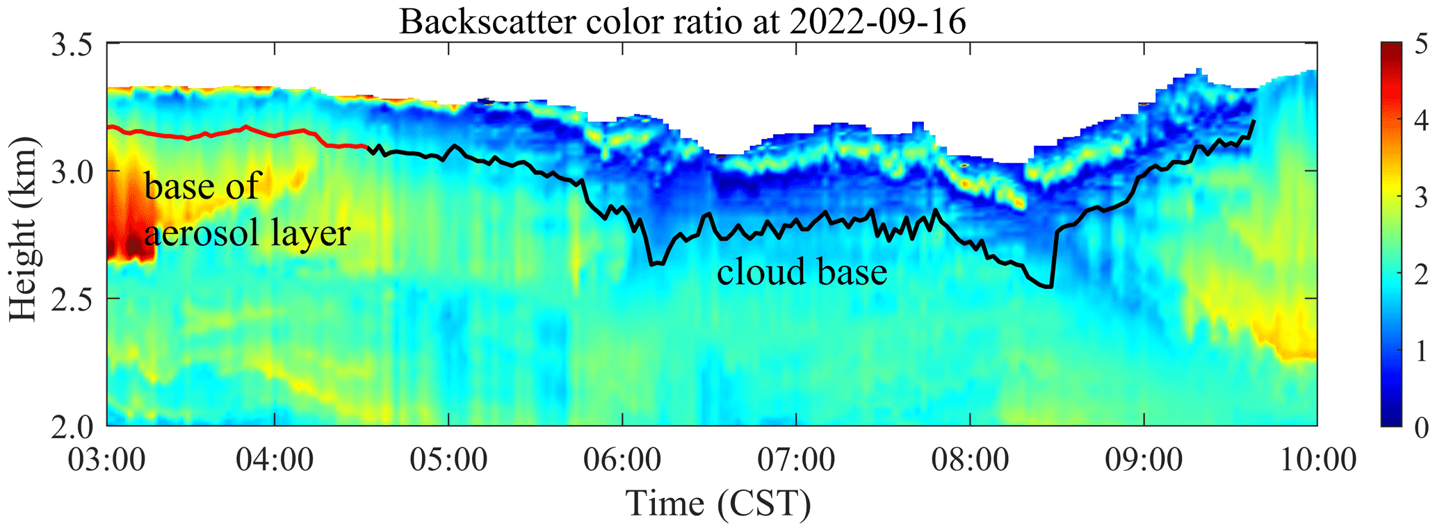
Figure 11Inversion results of backscatter color ratio at 03:00–10:00 CST on 16 September 2022.
Figure 12 shows the changes in the effective radius and particle number concentration (displayed in logarithmic form). The observation results can be separated into four stages, marked as 1, 2, 3, and 4 in Fig. 12. There are no clouds in regions 1 and 2, but based on the lidar echo signal, we can see a more obvious signal growth and change process. In stage 1, from 03:00 to 04:30 CST, clouds have not yet formed, but an obvious layer of aerosol at 3.2 km, with an average thickness of 180 m, can be seen. The effective radius and number concentration are relatively small, ranging from 1.2 to 1.5 µm and from 8.5 to 20.6 cm−3. In stage 2, from 04:30 to 05:06 CST, during which time the echo signal of the lidar is enhanced, the particle radius increases, and the effective radius increases to 1.4–1.8 µm. The concentration range is 13.3–25.6 cm−3. In stage 3, from 05:00 to 08:30 CST, cloud droplets are generated, and a cloud layer appears. The echo signal intensifies sharply, and the effective radius and number concentration increase significantly, with the effective radius being 1.5–5.3 µm and the concentration being 18.7–2853.5 cm−3. Due to the increase in number concentration, the laser cannot penetrate the cloud layer. In stage 4, from 08:30 to 10:00 CST, the cloud layer rises, and the cloud base height increases from 2.5 to 3.27 km. The effective radius inside the cloud remains unchanged, but the numerical concentration decreases. At 09:40 CST, the cloud signal disappeared, possibly due to the cloud leaving the field of view of the lidar, and thus became unable to be observed.
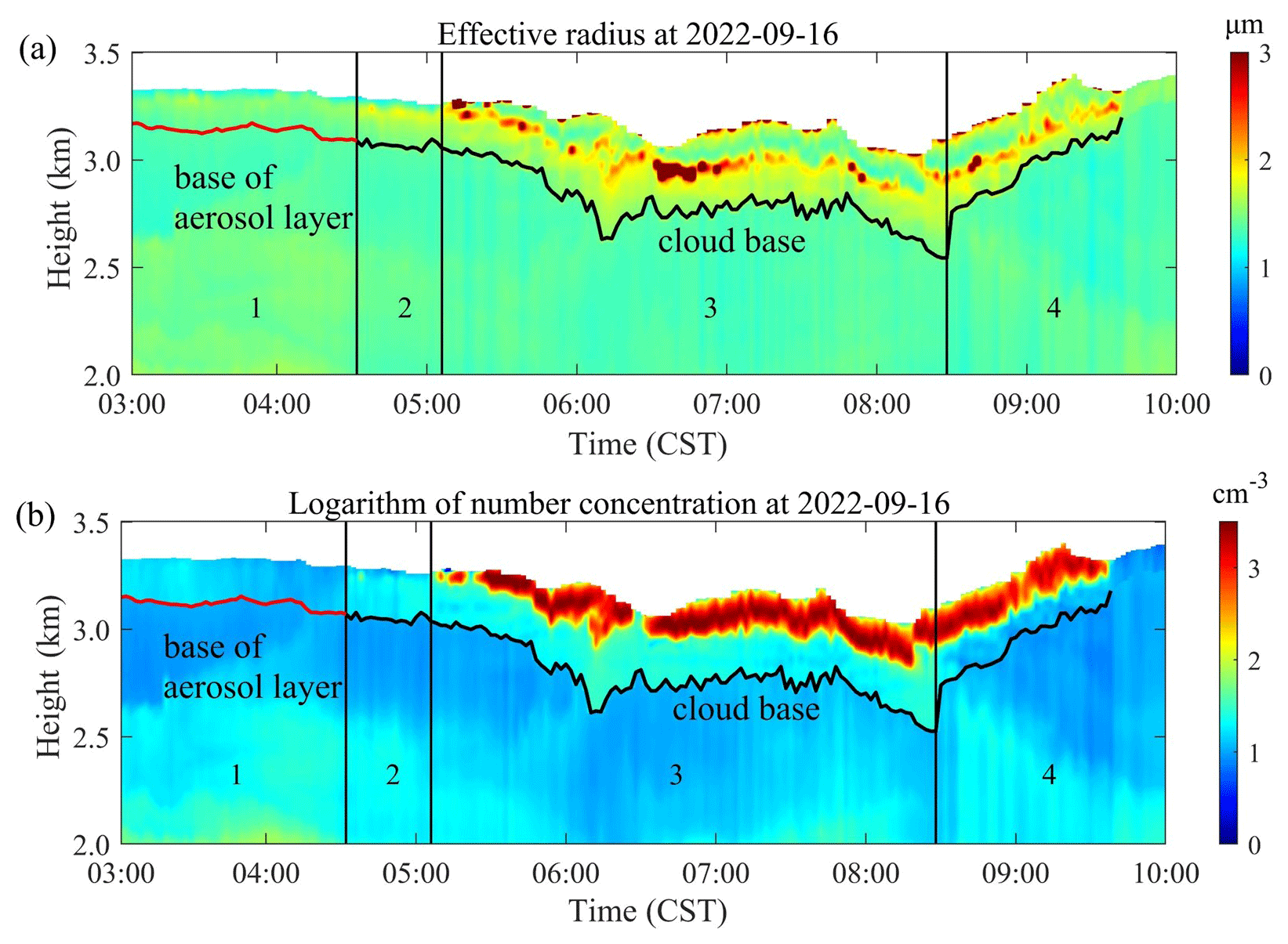
Figure 12Microphysical-parameter inversion results of atmospheric particulate matter at 03:00–10:00 CST on 16 September 2022. (a) Effective radius. (b) Number concentration.
This study proposes a method to estimate the microphysical parameters of atmospheric aerosols and small cloud droplets using two optical parameters. Assuming a gamma distribution, the effective radius and number concentration of aerosol or small cloud droplets can be calculated using the backscatter color ratios of 355 and 1064 nm wavelengths. An atmospheric-observation experiment was conducted using the multi-wavelength lidar, and the effective radius and number concentration were retrieved. The results indicate that the algorithm is stable and reliable.
This algorithm has simple hardware requirements for lidar, requiring only two wavelengths to achieve the retrieval of microphysical parameters. At the same time, the algorithm is simple and can obtain stable data inversion results. It is suitable for the retrieval of cloud droplet generation processes and aerosol with uniform mixing and relatively stable composition. The limitation of this algorithm is that it requires assuming the complex refractive index of particles. The complex refractive index of aerosol varies greatly, and incorrect assumptions about the complex refractive index can have a certain impact on the results. Furthermore, this algorithm is not applicable for the retrieval of large particle sizes (radius > 10 µm). To detect larger particle sizes, millimeter-wave cloud radar and lidar can be used for joint observation. We will carry out this work in the future.
The data and codes related to this article are available upon request from the corresponding author.
Conceptualization: HD. Investigation: XW and HD. Methodology: HD and XW. Software: XW and NC. Writing – original draft: XW and HD. Writing – review and editing: HD, DH. Supervision: HD and JG. Data collation: WX, SL, YG, QY, and YW. Project administration: HD and DH.
The contact author has declared that none of the authors has any competing interests.
Publisher's note: Copernicus Publications remains neutral with regard to jurisdictional claims made in the text, published maps, institutional affiliations, or any other geographical representation in this paper. While Copernicus Publications makes every effort to include appropriate place names, the final responsibility lies with the authors.
We express our gratitude to Mei Cao from the Xi'an Meteorology Bureau of Shaanxi Province, Xi'an, for providing the relevant supporting data.
This research has been supported by the National Natural Science Foundation of China (grant nos. 42130612 and 41627807).
This paper was edited by Alexander Kokhanovsky and reviewed by three anonymous referees.
Cai, Z. X., Li, Z. Q., Li, P. R., Li, J. X., Sun, H. P., Yang, Y. M., Gao, X., Ren, G., Ren, R. M., and Wei, J.: Vertical Distributions of Aerosol and Cloud Microphysical Properties and the Aerosol Impact on a Continental Cumulus Cloud Based on Aircraft Measurements from the Loess Plateau of China, Atmos. Environ., 270, 118888, https://doi.org/10.1016/j.atmosenv.2021.118888, 2022.
de Graaf, M., Apituley, A., and Donovan, D. P.: Feasibility study of integral property retrieval for tropospheric aerosol from Raman lidar data using principle component analysis, Appl. Optics, 52, 2173–2186, https://doi.org/10.1364/AO.52.002173, 2013.
Di, H. G., Wang, Q. Y., Hua, H. B., Li, S. W., Yan, Q., Liu, J. J., Song, Y. H., and Hua, D. X.: Aerosol Microphysical Particle Parameter Inversion and Error Analysis Based on Remote Sensing Data, Remote Sens.-Basel, 10, 1753, https://doi.org/10.3390/rs10111753, 2018a.
Di, H. G., Zhao, J., Zhao, X., Zhang, Y. X., Wang, Z. X., Wang, X. W., Wang, Y. F., Zhao, H., and Hua, D. X.: Parameterization of aerosol number concentration distributions from aircraft measurements in the lower troposphere over Northern China, J. Quant. Spectrosc. Ra., 218, 46–53, https://doi.org/10.1016/j.jqsrt.2018.07.009, 2018b.
Ding, J. F., Tian, W. S., Xiao, H., Cheng, B., Liu, L., Sha, X. Z., Song, C., Sun, Y., ang Shu, W. X.: Raindrop size distribution and microphysical features of the extremely severe rainstorm on 20 July 2021 in Zhengzhou, China, Atmos. Res., 289, 106739, https://doi.org/10.1016/j.atmosres.2023.106739, 2023.
Dionisi, D., Barnaba, F., Diémoz, H., Di Liberto, L., and Gobbi, G. P.: A multiwavelength numerical model in support of quantitative retrievals of aerosol properties from automated lidar ceilometers and test applications for AOT and PM10 estimation, Atmos. Meas. Tech., 11, 6013–6042, https://doi.org/10.5194/amt-11-6013-2018, 2018.
Gao, P., Wang, J., Tang, J. B., Gao, Y. Z., Liu, J. J., Yan, Q., and Hua, D. X.: Investigation of cloud droplets velocity extraction based on depth expansion and self-fusion of reconstructed hologram, Opt. Express, 30, 18713–18729, https://doi.org/10.1364/OE.458947, 2022a.
Gao, P., Wang, J., Gao, Y. Z., Liu, J. J., and Hua, D. X.: Observation on the Droplet Ranging from 2 to 16 µm in Cloud Droplet Size Distribution Based on Digital Holography, Remote Sens.-Basel, 14, 2414, https://doi.org/10.3390/rs14102414, 2022b.
Hara, Y., Nishizawa, T., Sugimoto, N., Osada, K., Yumimoto, K., Uno, I., Kudo, R., and Ishimoto, H.: Retrieval of Aerosol Components Using Multi-Wavelength Mie-Raman Lidar and Comparison with Ground Aerosol Sampling, Remote Sens.-Basel, 10, 937, https://doi.org/10.3390/rs10060937, 2018.
He, Y., Sun, Y. L., Wang, Q. Q., Zhou, W., Xu, W. Q., Zhang, Y. J., Xie, C. H., Zhao, J., Du, W., Qiu, Y. M., Lei, L., Fu, P. Q., Wang, Z. F., and Worsnop, D. R.: A Black Carbon-Tracer Method for Estimating Cooking Organic Aerosol from Aerosol Mass Spectrometer Measurements, Geophys. Res. Lett., 46, 8474–8483, https://doi.org/10.1029/2019GL084092, 2019.
Johnson, B. T., Christopher, S., Haywood, J. M., Osborne, S. R., McFarlane, S., Hsu, C., Salustro, C., and Kahn, R.: Measurements of aerosol properties from aircraft, satellite and ground-based remote sensing: a case-study from the Dust and Biomass burning Experiment (DABEX), Q. J. Roy. Meteor. Soc., 135, 922–934, https://doi.org/10.1002/qj.420, 2009.
Kanitz, T., Ansmann, A., Engelmann, R., and Althausen, D.: North-south cross sections of the vertical aerosol distribution over the Atlantic Ocean from multiwavelength Raman/polarization Lidar during Polarstern cruises, J. Geophys. Res.-Atmos., 118, 2643–2655, https://doi.org/10.1002/jgrd.50273, 2013.
Kaufman, Y. J., Hobbs, P. V., Kirchhoff, V. W. J. H., Artaxo, P., Remer, L. A., Holben, B. N., King, M. D., Ward, D. E., Prins, E. M., Longo, K. M., Mattos, L. F., Nobre, C. A., Spinhirne, J. D., Ji, Q., Thompson, A. M., Gleason, J. F., Christopher, S. A., and Tsay, S.-C.: Smoke, clouds, and radiation-Brazil (SCAR-B) experiment, J. Geophys. Res.-Atmos., 103, 31783–31808, https://doi.org/10.1029/98JD02281, 1998.
Kolgotin, A., Müller, D., and Romanov, A.: Particle Microphysical Parameters and the Complex Refractive Index from 3β+2α HSRL/Raman Lidar Measurements: Conditions of Accurate Retrieval, Retrieval Uncertainties and Constraints to Suppress the Uncertainties, Atmosphere-Basel, 14, 1159, https://doi.org/10.3390/atmos14071159, 2023.
Kulmala, M., Vehkamaki, H., Petaja, T., Maso, D. M., Lauri, A., Kerminen, V. M., Birmili, W., and McMurry, P. H.: Formation and growth rates of ultrafine atmospheric particles: A review of observations, J. Aerosol Sci., 35, 143–176, https://doi.org/10.1016/j.jaerosci.2003.10.003, 2004.
Li, L., Li, C. C., Zhao, Y. M., Li, J., and Chu, Y. Q.: Geometrical constraint experimental determination of Raman lidar overlap profile, Appl. Optics, 55, 4924–4928, https://doi.org/10.1364/AO.55.004924, 2016.
Lohmann, U. and Feichter, J.: Global indirect aerosol effects: a review, Atmos. Chem. Phys., 5, 715–737, https://doi.org/10.5194/acp-5-715-2005, 2005.
Meskhidze, N., Sutherland, B., Ling, X., Dawson, K., Johnson, M. S., Henderson, B., Hostetler, C. A., and Ferrare, R. A.: Improving Estimates of PM2.5 Concentration and Chemical Composition by Application of High Spectral Resolution Lidar (HSRL) and Creating Aerosol Types from Chemistry (CATCH) Algorithm, Atmos. Environ., 250, 118250, https://doi.org/10.1016/j.atmosenv.2021.118250, 2021.
Miffre, A., Abou Chacra, M., Geffroy, S., Rairoux, P., Soulhac, L., Perkins, R. J., and Frejafon, E.: Aerosol load study in urban area by Lidar and numerical model, Atmos. Environ., 44, 1152–1161, https://doi.org/10.1016/j.atmosenv.2009.12.031, 2010.
Moore, R. H., Wiggins, E. B., Ahern, A. T., Zimmerman, S., Montgomery, L., Campuzano Jost, P., Robinson, C. E., Ziemba, L. D., Winstead, E. L., Anderson, B. E., Brock, C. A., Brown, M. D., Chen, G., Crosbie, E. C., Guo, H., Jimenez, J. L., Jordan, C. E., Lyu, M., Nault, B. A., Rothfuss, N. E., Sanchez, K. J., Schueneman, M., Shingler, T. J., Shook, M. A., Thornhill, K. L., Wagner, N. L., and Wang, J.: Sizing response of the Ultra-High Sensitivity Aerosol Spectrometer (UHSAS) and Laser Aerosol Spectrometer (LAS) to changes in submicron aerosol composition and refractive index, Atmos. Meas. Tech., 14, 4517–4542, https://doi.org/10.5194/amt-14-4517-2021, 2021.
Müller, D., Wandinger, U., and Ansmann, A.: Microphysical particle parameters from extinction and backscatter lidar data by inversion with regularization: theory, Appl. Optics, 38, 2346–2357, https://doi.org/10.1364/AO.38.002346, 1999.
Müller, D., Hostetler, C. A., Ferrare, R. A., Burton, S. P., Chemyakin, E., Kolgotin, A., Hair, J. W., Cook, A. L., Harper, D. B., Rogers, R. R., Hare, R. W., Cleckner, C. S., Obland, M. D., Tomlinson, J., Berg, L. K., and Schmid, B.: Airborne Multiwavelength High Spectral Resolution Lidar (HSRL-2) observations during TCAP 2012: vertical profiles of optical and microphysical properties of a smoke/urban haze plume over the northeastern coast of the US, Atmos. Meas. Tech., 7, 3487–3496, https://doi.org/10.5194/amt-7-3487-2014, 2014.
Siomos, N., Balis, D. S., Poupkou, A., Liora, N., Dimopoulos, S., Melas, D., Giannakaki, E., Filioglou, M., Basart, S., and Chaikovsky, A.: Investigating the quality of modeled aerosol profiles based on combined lidar and sunphotometer data, Atmos. Chem. Phys., 17, 7003–7023, https://doi.org/10.5194/acp-17-7003-2017, 2017.
Veselovskii, I., Kolgotin, A., Griaznov, V., Müller, D., Wandinger, U., and Whiteman, D. N.: Inversion with regularization for the retrieval of tropospheric aerosol parameters from multiwavelength lidar sounding, Appl. Optics, 41, 3685–3699, https://doi.org/10.1364/AO.41.003685, 2002.
Veselovskii, I., Kolgotin, A., Griaznov, V., Müller, D., Franke, K., and Whiteman, D. N.: Inversion of multiwavelength Raman lidar data for retrieval of bimodal aerosol size distribution, Appl. Optics, 43, 1180–1195, https://doi.org/10.1364/AO.43.001180, 2004.
Veselovskii, I., Whiteman, D. N., Kolgotin, A., Andrews, E., and Korenskii, M.: Demonstration of aerosol property profiling by multi-wavelength lidar under varying relative humidity conditions, J. Atmos. Ocean. Tech., 26, 1543–1557, https://doi.org/10.1175/2009JTECHA1254.1, 2009.
Veselovskii, I., Dubovik, O., Kolgotin, A., Korenskiy, M., Whiteman, D. N., Allakhverdiev, K., and Huseyinoglu, F.: Linear estimation of particle bulk parameters from multi-wavelength lidar measurements, Atmos. Meas. Tech., 5, 1135–1145, https://doi.org/10.5194/amt-5-1135-2012, 2012.
Vivekanandan, J., Ghate, V. P., Jensen, J. B., Ellis, S. M., and Schwartz, M. C.: A Technique for Estimating Liquid Droplet Diameter and Liquid Water Content in Stratocumulus Clouds Using Radar and Lidar Measurements, J. Atmos. Ocean. Tech., 37, 2145–2161, https://doi.org/10.1175/JTECH-D-19-0092.1, 2020.
Wang, N., Zhang, K., Shen, X., Wang, Y., Li, J., Li, C., Mao, J., Malinkad, A., Zhao, C., Russellf, L., Guo, J., Gross, S., Liu, C., Yang, J., Chen, F., Wu, L., Chen, S., Ke, J., Xiao, D., Zhou, Y., Fang, J., and Liu, D.: Dual-field-of-view high-spectral-resolution lidar: Simultaneous profiling of aerosol and water cloud to study aerosol–cloud interaction, P. Natl. Acad. Sci. USA, 119, e2110756119, https://doi.org/10.1073/pnas.2110756119, 2022.
Wang, X. H., Di, H. G., Wang, Y. Y., Yin, Z. Z., Yuan, Y., Yang, T., Yan, Q., Li, S. C., Xin, W. H., and Hua, D. X.: Correction Method of Raman Lidar Overlap Factor Based on Aerosol Optical Parameters, Acta Optica Sinica, 43, 0601005, https://doi.org/10.3788/AOS221295, 2023a.
Wang, X. H., Li, S. W., Hui, G. D., Li, Y., Wang, Y. Y., Yan, Q., Xin, W. H., Yuan, Y., and Hua, D. X.: Calibration method of Fernald inversion for aerosol backscattering coefficient profiles via multi-wavelength Raman-Mie lidar, Opt. Commun., 528, 129030, https://doi.org/10.1016/j.optcom.2022.129030, 2023b.
Wang, Z. and Sassen, K.: Cirrus Cloud Microphysical Property Retrieval Using Lidar and Radar Measurements. Part I: Algorithm Description and Comparison with In Situ Data, J. Appl. Meteorol., 41, 218–229, https://doi.org/10.1175/1520-0469, 2002.
Zhao, C. F., Qiu, Y. M., Dong, X. B., Wang, Z. E., Peng, Y. R., Li, B. D., Wu, Z. H., and Wang, Y.: Negative aerosol-cloud relationship from aircraft observations over Hebei, China, Earth and Space Science, 5, 19–29, https://doi.org/10.1002/2017EA000346, 2018.
Zhang, Y., Chen, S., Tan, W., Chen, S., Chen, H., Guo,P., Sun, Z., Hu, R., Xu, Q., Zhang, M., Hao, W., and Bu, Z.: Retrieval of Water Cloud Optical and Microphysical Properties from Combined Multiwavelength Lidar and Radar Data, Remote Sens.-Basel, 13, 4396, https://doi.org/10.3390/rs13214396, 2021.
- Abstract
- Introduction
- Gamma distribution statistical characteristics of APSD and CDSD
- The inversion method for microphysical parameters of atmospheric aerosols or small cloud droplets
- Experiment
- Conclusions and discussion
- Code and data availability
- Author contributions
- Competing interests
- Disclaimer
- Acknowledgements
- Financial support
- Review statement
- References