A versatile water vapor generation module for vapor isotope calibration and liquid isotope measurements

A versatile vapor generation module has been developed for both field-based water vapor isotope calibrations and laboratory-based liquid water isotope measurements. The vapor generation module can generate a stream of constant vapor at a wide variety of humidity levels spanning 300 to 30 000 ppmv and is fully scalable, allowing in principle an unlimited number of standards or samples to be connected to a water vapor isotope analyzer. This versatility opens up the possibility for calibrating with multiple standards during field deployment, including examining instrument humidity–isotope dependence. Utilizing the ability to generate an uninterrupted constant stream of vapor, we document an Allan deviation for ¹⁷O-excess (Δ¹⁷O) of less than 2 per meg for an approximate 3 h averaging time. For similar averaging time, the Allan deviations for δ¹⁷O, δ¹⁸O, δD, and d-excess are 0.004 ‰, 0.005 ‰, 0.01 ‰, and 0.04 ‰, respectively. Measuring unknown samples shows that it is possible to obtain an average standard deviation of 3 per meg for Δ¹⁷O and an average standard error (95 % confidence limit) of 5 per meg.

Using the vapor generation module, we document that an increase in the Allan deviation above the white noise level for integration times between 10 min and 1 h is caused by cyclic variations in the cavity temperature, which if improved upon could result in an improvement in liquid sample measurement precision of up to a factor of 2. We further argue that increases in Allan deviation for longer averaging times could be a result of memory effects and not only driven by instrumental drifts as it is often interpreted.

The vapor generation module as a calibration system has been documented to generate a constant water vapor stream for more than 90 h, showing the feasibility of being used to integrate measurements over much longer periods than achievable with syringe-based injections as well as allowing the analysis of instrument performance and noise. Using clean in-house standards, we have operated the vapor generation module daily for 1–3 h for more than 6 months without the need for maintenance, illustrating its potential as a field-deployed autonomous vapor isotope calibration unit. When operating the vapor generation module for laboratory-based liquid water isotope measurements, we document a more than 2 times lower memory effect compared to a standard autosampler system.

1 Introduction

Water samples from the atmospheric hydrological cycle in the states of liquid, solid, and vapor offer an extraordinary tool for understanding how meteorological and hydrological processes drive the climate system. The isotopic composition of meteoric water represents integrated information of the water cycle from evaporation at the ocean and land surface along the air mass trajectory until the water molecules in the end fall back to the surface either as liquid or solid precipitation (e.g., Galewsky et al., 2016).

The relative abundance of HD¹⁶O and ${{\mathrm{H}}_{\mathrm{2}}}^{\mathrm{18}}\mathrm{O}$ compared to ${{\mathrm{H}}_{\mathrm{2}}}^{\mathrm{16}}\mathrm{O}$ of meteoric water samples has routinely been measured for more than the last 60 years (e.g., Craig and Gordon, 1965; Dansgaard, 1964). In recent decades the relative abundance of ${{\mathrm{H}}_{\mathrm{2}}}^{\mathrm{17}}\mathrm{O}$ compared with ${{\mathrm{H}}_{\mathrm{2}}}^{\mathrm{18}}\mathrm{O}$ has also been measured (e.g., Steig et al., 2014; Luz and Barkan, 2005). The relative abundance of HD¹⁶O, ${{\mathrm{H}}_{\mathrm{2}}}^{\mathrm{17}}\mathrm{O}$, ${{\mathrm{H}}_{\mathrm{2}}}^{\mathrm{18}}\mathrm{O}$ compared to ${{\mathrm{H}}_{\mathrm{2}}}^{\mathrm{16}}\mathrm{O}$, referred to using δ notation (Craig, 1961), is classically understood through the first-order principle of temperature-driven distillation during transport in the atmosphere (Dansgaard, 1964). To account for kinetic processes during phase transition, e.g., during ocean evaporation (Merlivat and Jouzel, 1979), formation of snow crystals (Jouzel and Merlivat, 1984), sublimation from snow (Wahl et al., 2021), or plant transpiration (Landais et al., 2006), second-order parameters such as the d-excess (Dansgaard, 1964) and the ¹⁷O-excess (Δ¹⁷O) (Landais et al., 2008) are defined:

$$\begin{array}{}\text{(1)}& {\displaystyle }\text{d-excess}=\mathit{\delta }\mathrm{D}-\left(\mathrm{8}\times \mathit{\delta }{}^{\mathrm{18}}\mathrm{O}\right),\text{(2)}& {\displaystyle }\mathrm{\Delta }{}^{\mathrm{17}}\mathrm{O}=\ln \left(\mathit{\delta }{}^{\mathrm{17}}\mathrm{O}+\mathrm{1}\right)-\mathrm{0.528}\ln \left(\mathit{\delta }{}^{\mathrm{18}}\mathrm{O}+\mathrm{1}\right).\end{array}$$

The number of atmospheric water vapor isotope measurements has over the last decade increased rapidly thanks to the availability of commercial water vapor isotope laser spectroscopy analyzers. Similarly, the number of laboratories that carry out routine measurements of liquid water samples for their isotopic composition has increased thanks to the lowering in costs of acquiring a laser spectroscopy analyzer and the ease of use compared to isotope ratio mass spectrometry (IRMS). This development has allowed the scientific community to enhance the understanding of the hydrological cycle by not only using collected precipitation samples, but also measuring the exchange and transport of water vapor in the climate system. However, the availability of high-accuracy water vapor isotope measurements has hinged on the ability to make robust and reliable field measurements of water vapor with known isotopic composition based on laboratory standards referenced against the international Vienna Standard Mean Ocean Water 2 – Standard Light Antarctic Precipitation 2 (VSMOW-SLAP) scale. Similarly, the availability of second-order parameters such as the d-excess or the Δ¹⁷O is dependent on the ability to make high-accuracy measurements of δ¹⁸O, δ¹⁷O, and δD.

Commercial systems including the Water Vapor Isotope Standard Source (WVISS) from Los Gatos Research and the Standard Delivery Module (SDM) from Picarro inc. have been developed together with commercial water vapor isotope analyzers. However, challenges in the calibration of measurements using these systems for long deployments (Bonne et al., 2014; Steen-Larsen et al., 2015) or deployments in low-humidity regions (Guilpart et al., 2017) have been documented. Custom-made changes to the SDM system have been carried out to facilitate long-term deployments (Bastrikov et al., 2014). While the SDM system allows two standards to be used, the WVISS system only allows a single standard to be measured without manually changing the standard. For the WVISS, this implies that a VSMOW-SLAP scale calibration cannot be performed automatically. For the SDM, this implies that the accuracy of the calibration cannot be assessed using a third known standard as is standard protocol for liquid water isotope measurements (e.g., van Geldern and Barth, 2012).

To overcome some of these challenges, custom-made calibration systems have been developed, specifically targeting the conditions of the field deployment. The simplest and to date most robust calibration system in terms of long-term deployment is the bubbler system, which has been used continuously at the water vapor isotope monitoring station in Bermuda for more than 10 years (Zannoni et al., 2022; Steen-Larsen et al., 2014). The versatility of the system lies in the wide humidity range (1000 to 30 000 ppm) and the minimal need for manual intervention to operate (e.g., Bailey et al., 2015; Ellehoj et al., 2013). However, for the system to operate with low uncertainty (providing calibration pulses with an uncertainty of ±0.1 ‰ and 1.0 ‰ for δ¹⁸O $/$ δD), it is a requirement that temperature stability to within half a degree is obtained. In addition, large quantities (3–5 L depending on deployment period) of water standards are needed, and it is not practical to transport or move during deployment. These constraints mean that the bubbler system is not feasible for many field campaigns.

Besides bubbler systems, custom-made calibration systems have been developed on the principle of either complete evaporation of small water droplets or steady-state evaporation of a sub-millimeter-sized droplet. The following belong to the former group of calibration systems: dew point generators (Lee et al., 2005), dripper systems (Tremoy et al., 2011; Lee et al., 2005), nebulizer systems (Jones et al., 2017), and piezoelectric microdrop generators (Iannone et al., 2009). While these systems have been proven to work under field conditions, they require significant time to equilibrate and may potentially be sensitive to room temperature fluctuations. For the operation of the nebulizer system, the system needs on the order of 5 L min⁻¹ dry air to achieve low-humidity levels, which provides an additional need for bringing a high-performance dry air generator into the field, which adds logistical challenges for organizing field campaigns.

The following belong to the group of calibration systems operating on the principles of steady-state evaporation: a field deployable system developed by Gkinis et al. (2011) for continuous ice core water isotope analysis directly in the field and a dedicated low-humidity calibration system developed by Leroy-Dos Santos et al. (2021). The system developed by Gkinis et al. (2011) used the combination of a peristaltic pump and tuned back pressure to push water through a silica capillary into a micro-tee heated to 170 °C. A similar system has also been deployed and used for calibration of water vapor isotope measurements (Benetti et al., 2017; Steen-Larsen et al., 2014). A similar system has also been shown to be reliable for Δ¹⁷O measurements in continuous-flow analysis of ice core samples (Davidge et al., 2022).

To achieve atmospheric water vapor and liquid sample data of the highest quality, it is crucial to address the sources of measurement uncertainty arising through both the measurement protocol and the instrumental drift. Several published protocols exist for liquid samples (e.g., Hutchings and Konecky, 2023; Penna et al., 2012; van Geldern and Barth, 2012) and atmospheric water vapor (e.g., Bailey et al., 2015; Steen-Larsen et al., 2013), along with a multitude of laboratory-specific protocols. However, improvement of liquid measurement protocols for better precision and accuracy has been restricted to adjusting the number of injections, the amount of injected liquid, and to a small degree changes in integration time. For measurement protocols of water vapor isotopes, improvements have been restricted by the lack of a possibility of generating a continuous vapor stream with constant and known isotopic composition at different humidity levels using more than two standards.

Our goal was to not only develop a field-deployable water vapor isotope calibration system targeting the shortcomings described above, but also develop a system for liquid sample measurements exceeding available systems in throughput and accuracy. To achieve this, we have further developed the vapor generation module for which a patent application was filed in 2015 and published in Steen-Larsen (2016). Our targets for the water vapor isotope calibration needs were

• field deployable (i.e., robust), transportable, and easy to operate;

• multiple standard measurement capability;

• wide humidity span from 300 to 30 000 ppmv;

• high flow rate span of vapor with a constant known isotopic composition;

• possibility to calibrate with sufficiently high accuracy for Δ¹⁷O data.

Our targets for the liquid measurements were

• scalable system in terms of the number of unknown samples,

• improvement in sample measurement time compared to discrete injections for similar precision,

• user-defined choice of integration time and hence measurement accurateness and precision,

• comparable sample material use as discrete measurements/small quantity of sample material.

The developed system should have the ability to be used for both liquid measurements and calibration of water vapor isotope measurements. In addition, the system should have sufficient stability to function as a benchmark tester for isotope analyzer performance by supplying a constant stream of water vapor with a known isotopic composition over multiple days.

To further demonstrate the fulfillment of all the proposed targets, we report two case studies as representative of water isotope calibration and liquid measurement applications:

• a humidity–isotope characterization curve performed during a field campaign in the Arctic and

• the liquid analysis of Δ¹⁷O of artificial samples generated from the mixing of two reference waters with known Δ¹⁷O values.

2 Materials and methods

2.1 Vapor generation module description

The vapor generation module is an improved and revised version of an original prototype developed in 2014 for which a patent application was filed in 2015 (Steen-Larsen, 2016). The previous prototype was re-engineered at the beginning of 2021, and its schematic with a generic number of ovens (n) is reported in Fig. 1. A four-oven version was used in this study. The focus of the improvements compared to the original prototype is the control of the liquid going into the oven and control over stopping the flow of liquid into the oven.

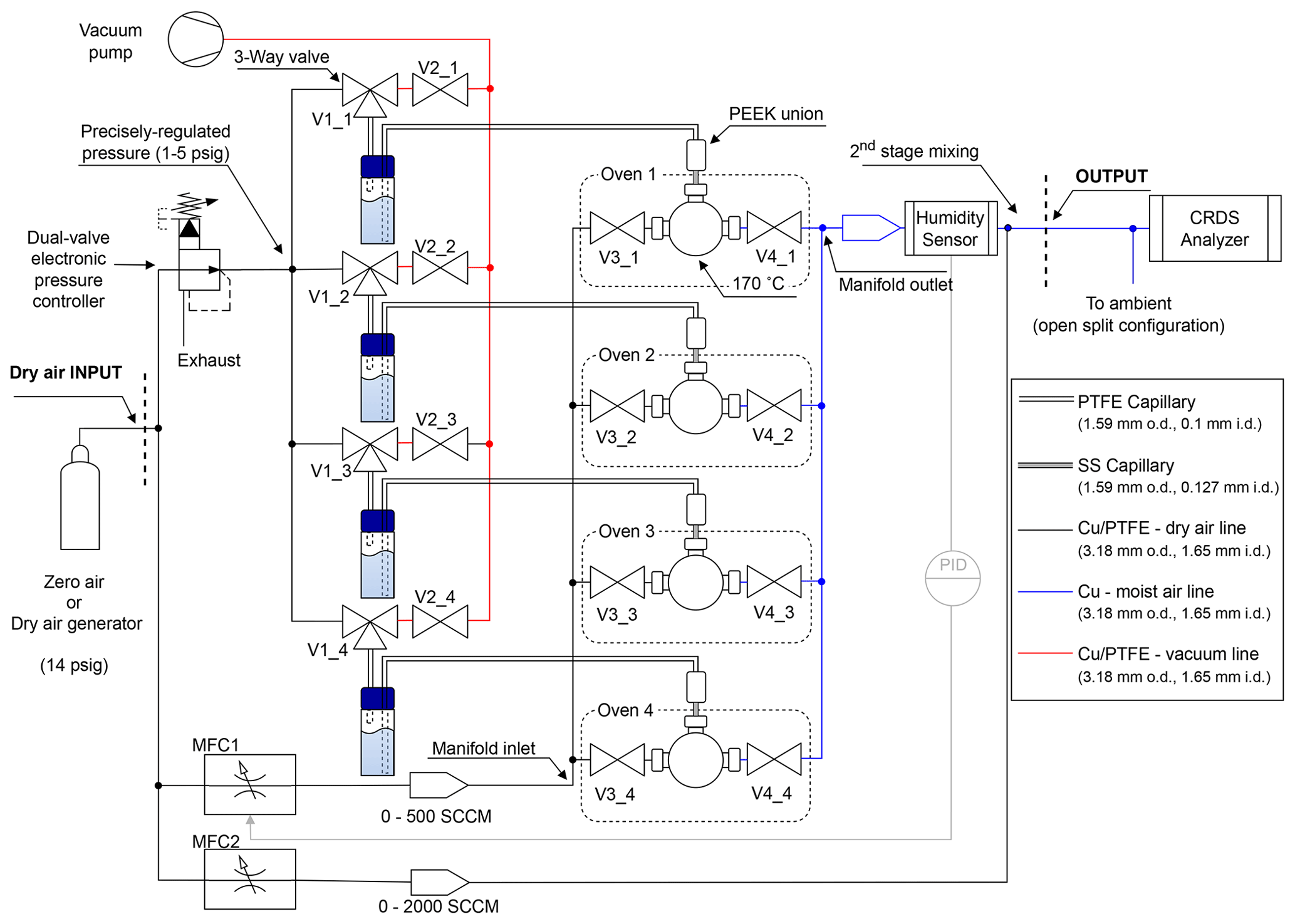
Figure 1 Diagram of the vapor generation module equipped with multiple ovens. The gas analyzer must be connected at the OUTPUT of the vapor generation module in open-split mode to allow the part of the vapor stream that is not going into the Picarro instrument to escape. Pictures of the physical realization of the vapor generation module are shown in Fig. S5 in the Supplement. Reference to product numbers of the labeled components is reported in Sect. S1 in the Supplement.

The operating principle of the vapor generation module is based upon the flash evaporator method, which is adopted in the water stable isotope community for continuous-flow analysis of ice cores and for atmospheric water vapor analysis (e.g., Gkinis et al., 2011; Leroy-Dos Santos et al., 2021). In the flash evaporator, a droplet of water continuously evaporates on the tip of a needle/capillary inside an evaporation chamber at high temperature. The temperature of the evaporation chamber is precisely controlled well above the boiling point (in this work at 170 °C), and the volume is continuously flushed with dry air to produce a water vapor stream with the same isotopic composition of the water source in the needle. As recently demonstrated, no fractionation occurs during operation in steady state, and back diffusion from the tip through the capillary line is not sufficient to affect the water vapor isotopic composition inside the water reservoir (Kerstel, 2021; Leroy-Dos Santos et al., 2021). To push the water through the capillary, previous studies used syringe pumps or combinations of tubing pieces of different sizes to generate sufficient back pressure (Gkinis et al., 2011; Landsberg et al., 2014; Leroy-Dos Santos et al., 2021). In this study, we used compressed dry air, with headspace pressure precisely controlled by an electronic pressure regulator (Alicat PCD-5PSIG, resolution 0.01 PSI or 70 Pa), as proposed in Steen-Larsen (2016).

The main improvements from the original design are the presence of the following:

• 1.

  a vacuum pump that can be connected to the vial headspace via a three-way valve and a vacuum valve to halt vapor generation in the oven,

• 2.

  a proportional–integral–derivative (PID) control loop to control and stabilize the humidity level,

• 3.

  an additional mixing tee connected (second stage mixing) to a secondary mass flow controller (MFC2) to ensure a larger dynamic humidity range,

• 4.

  the use of a dual-valve pressure controller flow meter to enable seamless control of the humidity level,

• 5.

  use of stainless-steel capillaries instead of fused silica capillary tubes,

• 6.

  the option of using a single oven connected to a selector valve connected to individual vials.

These main improvements compared to the original patent application (Steen-Larsen, 2016) were implemented with the following operations in mind. (1) The purpose of the vacuum pump is to create a small vacuum in the vials' headspace, which reverses the flow of the water in the capillaries out of each oven and back into the vials. The benefit of this is that water is immediately removed from the capillary, and the oven dries out immediately, minimizing cross-contamination of the samples and build-up of water inside the oven. (2) A custom humidity sensor probe is installed in the tube where the vapor is flowing to the analyzer and internally looped to the primary MFC to control the humidity level. This is necessary because of the potential for a slowly decreasing trend of humidity during long injection time (several hours). The decrease in injection performance during long runs is attributed to the build-up of salt deposits inside the capillary during evaporation (further discussed in Sect. 4.3). (3) The secondary MFC allows for a second dry air stream to be mixed into the flow of vapor from the oven at a higher flow rate than the primary MFC and without influencing the production of vapor in the oven. This way, the vapor generation module can generate humidity levels at a much lower level compared to using only mixing in the oven setup and can also generate vapor with a higher flow rate. (4) The dual-valve pressure controller flow meter installed to regulate the pressure in the vials' headspace is chosen to ensure that the pressure can be both increased and decreased. (5) As discussed in Sect. 4.3, one of the main issues with the operation of a flash evaporator of this type is clogging of the capillaries. We observed that the use of stainless-steel capillaries reduced the frequency of clogging compared to using fused silica capillaries. (6) Instead of having individual ovens and valve circuits for each sample vial, we installed a selector valve similar to Jones et al. (2017) for the purpose of cost optimization (see Fig. S1 in the Supplement). Unfortunately, the use of a selector valve comes at the cost of an increased memory effect between samples; hence, we opted for a combination of individual ovens and valve circuits with the use of a 10-port selector valve. For generating a stream of water vapor from standards, we use the individual oven and valve circuits while liquid samples are measured using the selector valve and single oven circuit.

2.2 Technical realization of the vapor generation module

For the technical realization of the vapor generation module, a 2 mL sample vial commonly used in autosamplers for liquid water isotope analysis was used as the water reservoir, as shown in Fig. 2a. A PTFE capillary (1.59 mm outer diameter, o.d.; 0.150 mm inner diameter, i.d.) is passed through a tee assembly and 3.18 mm o.d. stainless-steel tubing (i.d. > 1.59 mm) toward the bottom of the vial, which is kept in place with a Swagelok UltraTorr fitting. The PTFE capillary is sealed only at the very top of the tee assembly with a PTFE ferrule and a PTFE nut to minimize the deformation of the PTFE capillary. The pressure inside the tee assembly is equal to the pressure in the vial headspace and can be precisely controlled either with a manual pressure regulator (model 8286, Parker) or an electronic dual-valve pressure controller (PCD-5PISG-D-SV, Alicat Scientific), which includes an advanced PID control of the pressure. Any change in the pressure in the headspace (positive or negative) will produce a flow of water through the PTFE capillary. In this study, the headspace pressure was regulated between 0.5 and 3.5 PSI.

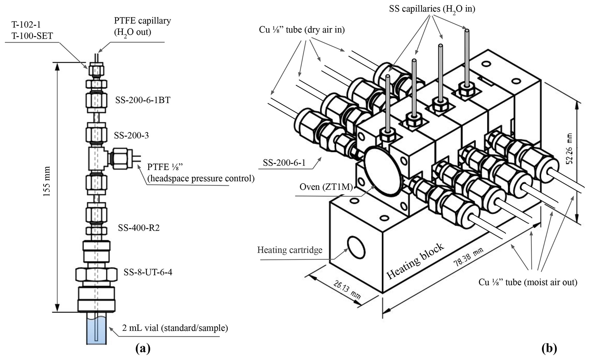
Figure 2 Technical drawings of the components used to produce the water vapor stream. (a) Details of the custom vial holder (with Swagelok part numbers). (b) Details of the compact 4-oven assembly (Swagelok and VICI part numbers).

The PTFE (polytetrafluoroethylene) capillary is connected with a 1.59 mm PEEK (polyether ether ketone) union to a 100 mm long stainless-steel capillary with 0.127 mm i.d. (T10C5, VICI) and fitted into one end of a stainless-steel tee (ZT1M, VICI) which is kept in place over a 200 W heating element (860-6912, RS-PRO) with a custom aluminum assembly, as shown in Fig. 2b. The stainless-steel tee and the heating block are placed into an aluminum die-cast enclosure (Hammond Manufacturing) and thermally insulated with machinable glass ceramic rods (Corning) and wrapped in fiberglass liner. As mentioned before, in this study we used a four-element version of the oven, but the module is highly scalable in terms of the number of heated tee units.

The water vapor produced in the oven is routed toward the output of the system through the stainless-steel valve manifold and a copper tube where the vapor is measured using a custom humidity sensor probe to monitor the temperature and the humidity of the outflow gas (AD22100STZ, Analog Devices, and HIH-4000-004, Honeywell, inside a SS-400-3-4TTF tee, Swagelok). The humidity sensor probe is used to control the flow rate of the first MFC (GFC17A, 0–500 mL min⁻¹, Aalborg Instruments) with a PID to keep a steady humidity level at the output of the vapor generation module during long injections. A data acquisition module (USB-6001, National Instrument) was used to control the valves and MFCs. The control software was written in LabView 16.

2.3 Continuous injections of different samples

In a subsequent modification of the vapor generation module, we used a single oven connected with the stainless-steel capillary to a multiport selector (C25-3180EUHA, VICI) to inject samples from the different vial holders continuously, without needing to switch the oven. This second modification was introduced to analyze samples of unknown isotopic composition in a similar fashion to continuous-flow analysis of ice cores. The possibility of changing between water sources without affecting the water vapor production enables both measurements of individual unknown samples and the possibility of running long stability tests (> 24 h) since switching between samples containing the same standard occurs seamlessly.

2.4 Standards and samples used for testing the vapor generation module

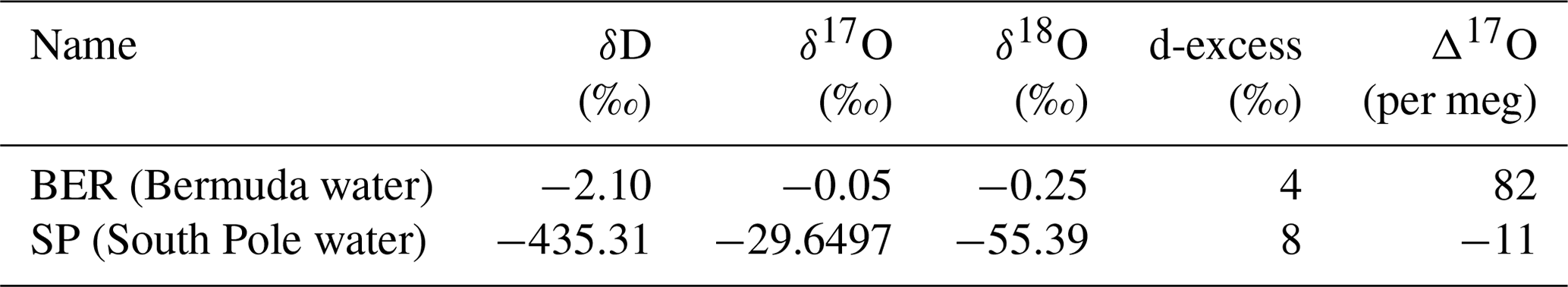
A wide range of isotopic values were used to test the calibration module, spanning approximately the VSMOW-SLAP range (Coplen, 1988; Gonfiantini, 1978). Laboratory standards with known isotopic composition for this study were provided by the Laboratoire des Sciences du Climat et de l'Environnement, the Centre for Ice and Climate at the Niels Bohr Institute, and the Stable Isotope Laboratory at the Institute of Arctic and Alpine Research, University of Colorado. The Δ¹⁷O values of the standards provided by the Stable Isotope Laboratory were provided by Δ^*IsoLab, University of Washington. An overview of all the standards used is listed in Table S1 in the Supplement, while Table 1 shows the most frequently used standards for analyzing stability and memory effects. Moreover, four more samples (Table S2) were prepared at the University of Bergen by weighing precise amounts of SW and WW standards (Table S1) with an uncertainty of 0.01 g to test the reproducibility of the Δ¹⁷O measurements. For these four samples, the uncertainty associated with the Δ¹⁷O value is assumed to be half the maximum span obtained by mixing SW ± 0.01 g with WW ± 0.01 g, which is approximately 0.013 ‰ (13 per meg).

Table 1 Standards used for stability and memory effect analysis in this study.

2.5 Isotopic water vapor analyzer

Most of the laboratory characterization tests for the vapor generation module were performed using a L2140-i cavity ring-down spectroscopy (CRDS) water isotope analyzer by Picarro (serial no. HKDS2156). In one occasion, to identify the source of measurement noise, the analyzer was run simultaneously with another Picarro L2140-i (serial no. HKDS2092). The HKDS2092 model was also used for the field activity mentioned in this work (see Sect. 3.4). Chronologically, the HKDS2092 is the oldest manufactured instrument that was used while HKDS2156 is the most recent one. Both the HKDS2092 and the HKDS2156 have an acquisition rate of ∼ 1 Hz, which is a typical value for this type of instrument. The reader is referred to previous studies for detailed descriptions of the technology and performances of such analyzers (e.g., Steig et al., 2014).

3 Results

3.1 Long-term injection and long-term stability

To demonstrate the long-term stability of the vapor generation system, a 92 h test was performed during the fall of 2022, from 10 October 16:20 to 14 October 12:25 LT (local time). During the test, a 2 mL aliquot of SP standard (1 vial) and a 26 mL aliquot of BER (13 vials) were injected using the four available vial holders and routed to a single oven using a multiport selector. The consumption rate was ∼ 1.5 µL min⁻¹. To prevent contamination between SP and BER standards, the first holder was only used for SP standards, while the remaining three were cycled every 24 h using fresh BER standards. Sequence, timing, and relevant statistics of the injections are reported in Table S3. The PID control loop was set to 17 300 ppmv, and the final averaged humidity recorded was 17 229 ± 340 ppmv with no observable trend, as shown in Fig. 3a. For ∼ 80 % of injections, the standard deviation of H₂O was between 113 and 353 ppmv, yielding a relative standard deviation in the range 0.7 %–2 %. There is apparently no pattern in the variability of H₂O signal among the different holders. At the working humidity between 15 000 and 20 000 ppmv, the humidity–isotope response curve is almost flat for δ¹⁷O and δ¹⁸O. The temporal evolution in the humidity, δ¹⁷O, δ¹⁸O, δD, d-excess, and Δ¹⁷O are shown in Fig. S2. A small dependency was observed between H₂O and δD, as reported in Fig. S3, but we do not correct for this.

The Allan deviation plots in Fig. 3b and c (solid lines) show a constant improvement of the two-sample variance, consistent with a nearly flat noise spectrum (white noise). For ideal white noise, a slope of −0.5${\mathit{\sigma }}_{\mathrm{Allan}}/\mathit{\tau }$ is expected. Observed slopes between averaging time 1 to 10⁴ s are −0.42 ‰, −0.33 ‰, −0.31 ‰, and −0.38 ‰ s⁻¹ for δ¹⁷O, δ¹⁸O, δD, and d-excess, respectively, as well as −0.42 ppm s⁻¹ for Δ¹⁷O. A slope lower than the one predicted for pure white noise implies that the non-flat spectral characteristic of the measurement noise can be due to the instability of the analyzer as well as from the instability of the vapor generation module. We note that for some ranges of averaging times, the measurement noise can be seen to be pure white noise. For example, white noise is observed for d-excess and Δ¹⁷O in the ranges 1 to 10² and 1 to 10¹ and again in the ranges 10³ to 2×10⁴ and 2×10² to 10⁴ s, respectively. In the range ∼ 10² to 10³ and ∼ 10¹ to 2×10² s for, respectively, d-excess and Δ¹⁷O, it can be noted that instabilities of the analyzer exist, which has consequences for the optimal choice of averaging time when weighing precision up against averaging time. It is worth noting that the Allan deviation plot presented in this study shows better isotopic analyzer performances than previously published in other studies (e.g., Sturm and Knohl, 2010; Steig et al., 2014; Leroy-Dos Santos et al., 2021; Aemisegger et al., 2012), yielding 0.004 ‰, 0.005 ‰, 0.01 ‰, and 0.04 ‰ σ_Allan for 10⁴ s averaging time for δ¹⁷O, δ¹⁸O, δD, and d-excess, respectively, as well as 2 per meg σ_Allan for 10⁴ s averaging time for Δ¹⁷O. Although for 10³ s, we show similar Δ¹⁷O σ_Allan values as Davidge et al. (2022). We argue that the apparent better performance is not only dependent on the isotope analyzer quality, even though instrumental performance improved with the introduction of the Picarro L2140-i series, but also dependent on the management of the memory effect during Allan deviation tests, such as priming the system for up to 12 h using the same standard. As mentioned above, the 92 h test started with a large positive isotopic step change in the water vapor source (∼ 55 ‰ for δ¹⁸O), and the following 16 h was removed from the Allan deviation analysis to minimize the memory effect. If the extra 16 h of data is used to compute the Allan deviation, the plateau is reached already at 4×10³ s, and the σ_Allan is larger (dashed lines in Fig. 3b). Most notably, an apparent drift effect shows up for δD after an averaging time of 10² s. Interestingly, the Δ¹⁷O quantity seems to be unaffected by this memory effect issue. To test the long-term stability and reproducibility of the Allan deviation characterization, an independent characterization was carried out 8 months later. The test revealed a similar result as presented in Fig. 3.

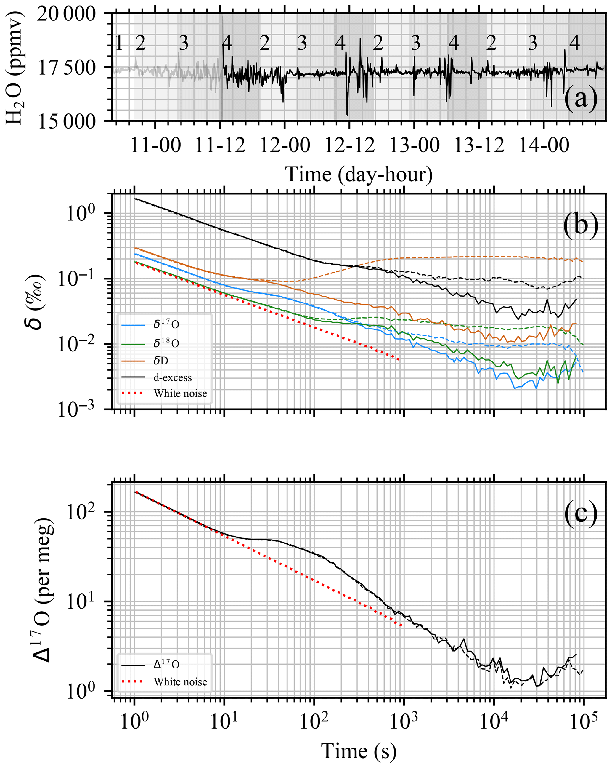
Figure 3 Flash evaporator 92 h stability test of the BER standard. (a) Time series of H₂O signal (17 229 ± 340 ppmv). The signal used to calculate the Allan deviation is reported as a solid black line. On the x axis are day (October 2022) and hour (LT). Gray shading is used to distinguish among injections from different vials. The IDs of vial holders are reported on the top of the plot. (b) Allan deviations of δ¹⁷O, δ¹⁸O, δD, and d-excess during the long-term stability test are shown, including the full 92 h dataset (dashed lines) and discarding the first 16 h (solid lines). The Allan deviation of white noise is reported as a dotted red line for reference. (c) Similar to panel (b) but for Δ¹⁷O.

3.2 Isotope step change and reduced memory effect

Assuming that 24 h of continuous injection of the same water standard is enough to completely remove the memory effect of the previous sample, we show in Fig. 4 the temporal evolution of the SP-BER normalized isotopic step change curve for fractions of the normalized target value larger than 0.90. For comparison, we ran a similar step-change test using the liquid injection mode of the Picarro L2140-i instrument (¹⁷O, high-precision mode) coupled to the A0235 autosampler and A0211 vaporizer. For the liquid injection test, the standards were analyzed as follows: two vials of SP (25 injections each) followed by nine vials of BER (25 injections each) for a total number of 275 injections and a running time of ∼ 41 h. Results clearly show that the vapor generation module is faster than the vaporizer using the autosampler system for reaching the target value after the step change. For instance, when using the vapor generation system, the 0.995 level is reached after 24, 23, and 47 min for δ¹⁷O, δ¹⁸O, and δD, respectively. The same level is reached with the vaporizer using the autosampler system after 54, 54, and 152 min. However, the liquid injections with the vaporizer using an autosampler are evenly spaced by cleaning cycles of the vaporizer, robotic arm movements, etc. All such operations require a considerable amount of time, which is mentioned hereafter as dead time. The large difference in the memory effect is discussed further in Sect. 4.4. Figure 4 shows that timings for the calibration system and vaporizer using the autosampler are comparable for δ¹⁷O and δ¹⁸O when dead time is ruled out. However, when theoretically removing the dead time, the vaporizer using the autosampler requires ∼ 77 min to reach the 0.995 level of target value for δD, which is still considerably longer by about ∼ 60 % than the time required by the presented vapor generation system.

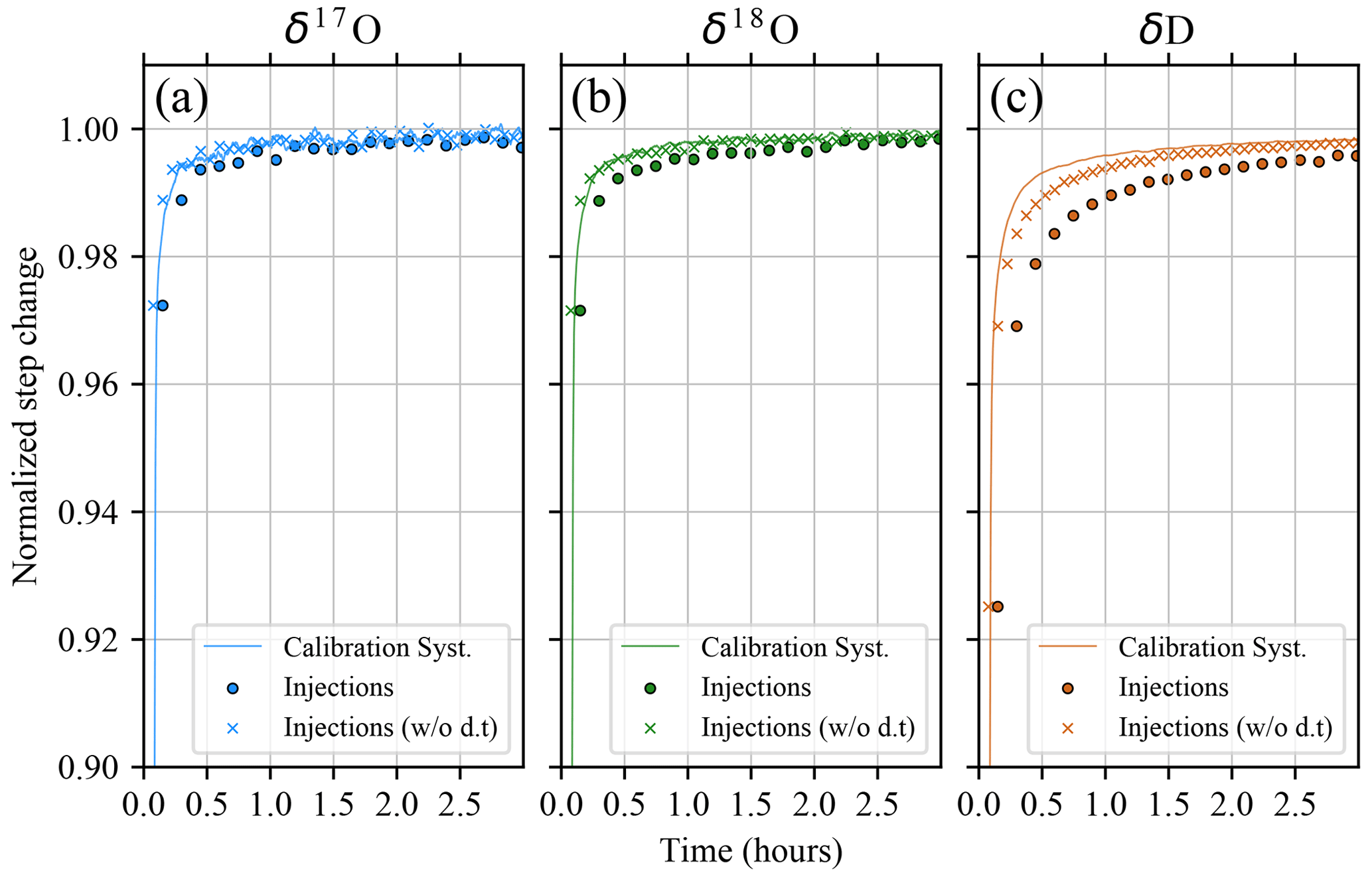
Figure 4 Normalized step change between standards SP and BER for (a) δ¹⁷O, (b) δ¹⁸O, and (c) δD, respectively. Solid lines: continuous signal acquired from the calibration system (moving average 270 s). Colored circles: injections performed with the Picarro autosampler and vaporizer including dead time (d.t). Colored crosses: injections performed with the Picarro autosampler and vaporizer removing dead time.

3.3 Short-term stability

The vapor generation module was tested by injecting the BER standard at 12 different humidity levels with injection times ranging from 3.5 to 8.7 h (see Fig. 5 and Table S4).

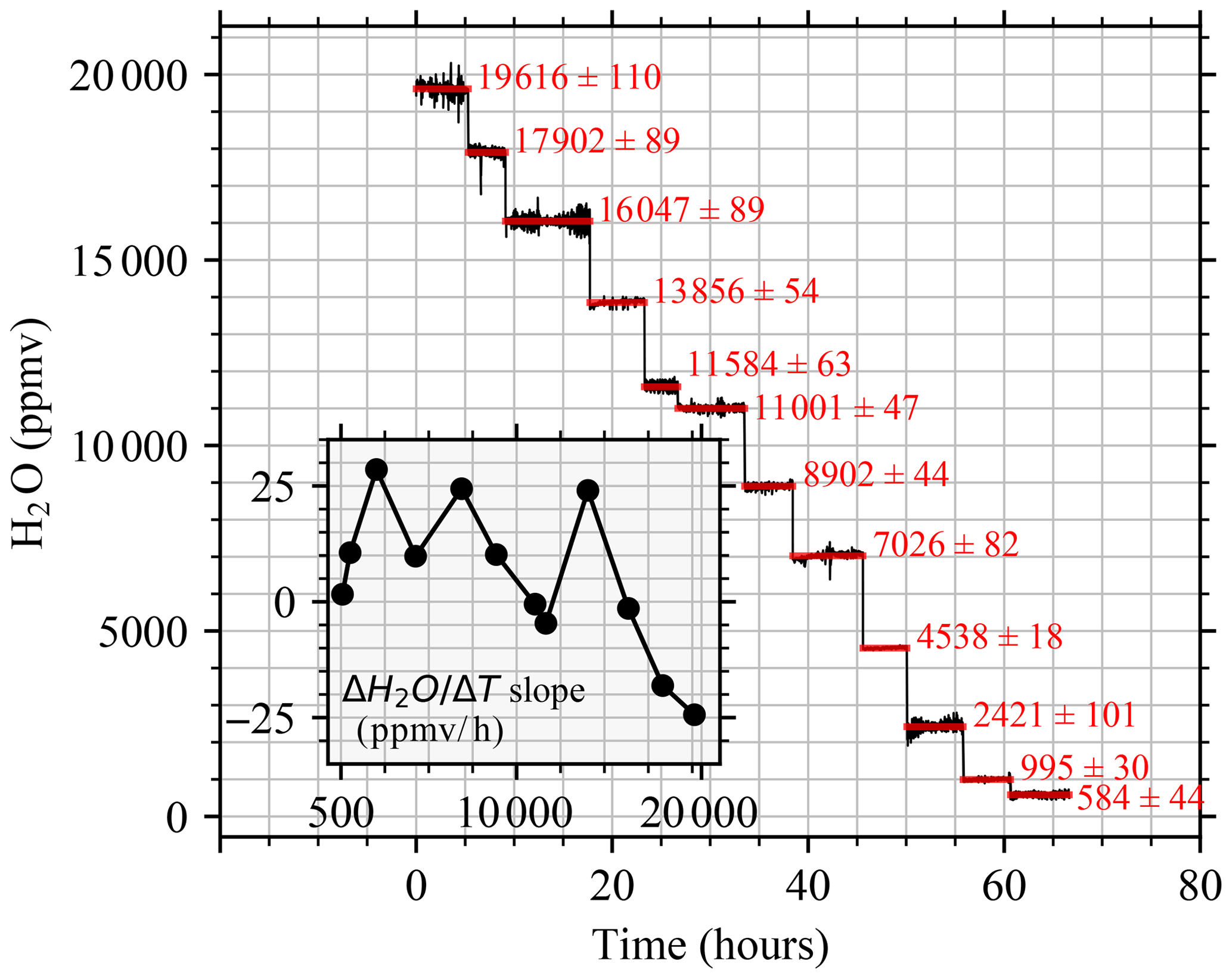
Figure 5 Humidity levels selected to test the short-term performances of the vapor generation module. H₂O 1σ_1−s is 1 standard deviation calculated at a standard sampling rate (∼ 1 Hz). The trend in the humidity level during each level is shown in the inset.

Such humidity levels almost completely cover the mixing ratio variability of the Earth's lower troposphere, with the exception of very dry regions like Antarctica (Casado et al., 2016) and warm-wet regions like tropical areas (e.g., Laskar et al., 2014). The stability of the water vapor signal was evaluated with three metrics for each level as follows.

3.3.1 Metric 1: the spread variability of the H₂O signal

Results in Fig. 5 show that the 1 s standard deviation ranges between 18 and 110 ppmv and is independent of the humidity level. If a smaller variability is required, the vapor generation module can be locked to a humidity level, and a second dry airflow can be used to dilute the water vapor concentration at the second tee (see “2nd stage mixing” in Fig. 1). The application study in Sect. 3.4 reports an example of usage of the second stage mixing and the associated 1 s standard deviation between humidity levels of 500–3500 ppmv.

3.3.2 Metric 2: the short-term trend of the H₂O signal (ΔH₂O $/$ Δt)

Results in Fig. 5 show that the trend, evaluated between 3.5 and 8.7 h, is limited to a narrow variation range from −24 to 29 ppmv h⁻¹. Positive trends were always observed below 9000 ppmv, while positive and negative trends were above 11 000 ppmv.

3.3.3 Metric 3: the overlapping Allan deviations of δ¹⁷O, δ¹⁸O, δD, and Δ¹⁷O

In general, a significant improvement in the two-sample variance can be observed above 5000 ppmv (Fig. A1). As expected, the largest Allan deviation with averaging time of 600 s is the one measured at the 584 ppmv level (0.04 ‰, 0.05‰, and 0.17‰ for δ¹⁷O, δ¹⁸O, and δD, respectively). Between 5000 and 20 000 ppmv, the 600 s Allan deviation is characterized in general by small variability (0.013 ‰ ± 0.002 ‰, 0.014 ‰ ± 0.004 ‰, and 0.02 ‰ ± 0.01 ‰ for δ¹⁷O, δ¹⁸O, and δD, respectively). For unknown reasons, the worst performances in terms of Allan deviation are observed at 11 584 ppmv (0.02 ‰, 0.03 ‰, and 0.06 ‰ for δ¹⁷O, δ¹⁸O, and δD, respectively for 600 s averaging time). This is in contrast with the analysis above, which shows the smallest short-term trend of the H₂O signal in the ∼ 12 500 ppmv region, which is ∼ 0 ppmv h⁻¹. Similar to δ¹⁷O, δ¹⁸O, and δD, the overlapping Allan deviation of Δ¹⁷O follows in general the same pattern, as shown in Fig. 6. However, the decrease in performances observed for δ¹⁷O, δ¹⁸O, and δD at 11 584 ppmv is limited for Δ¹⁷O. The optimal working region of the Picarro L2140i coupled to the vapor generation module is between 14 000 and 18 000 ppmv.

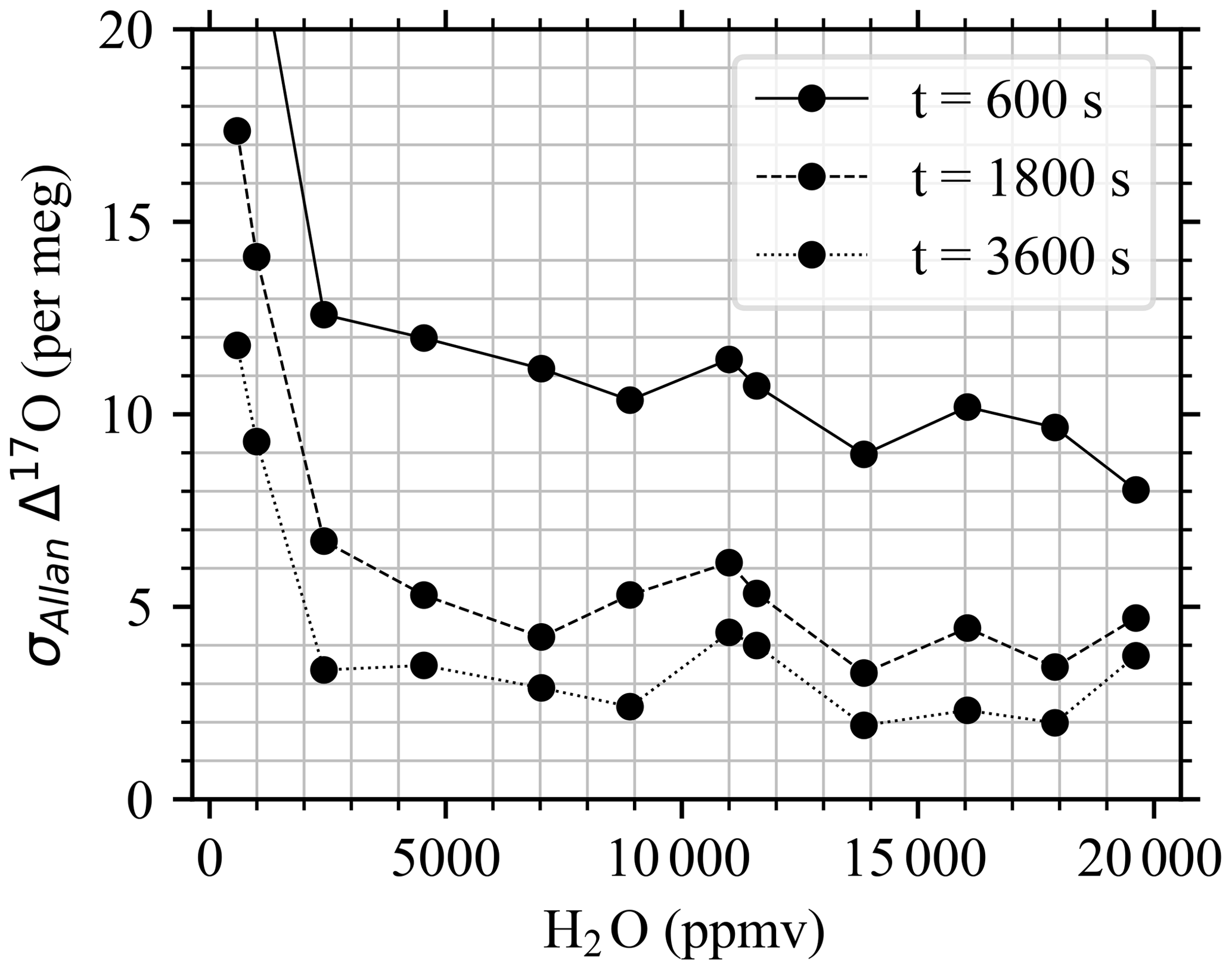
Figure 6 Overlapping Allan deviations of Δ¹⁷O measured at different humidity levels and for different integration times.

3.4 Application study 1: humidity–isotope characterization of the water vapor analyzer for the lower polar troposphere (WIFVOS)

Obtaining accurate vertically resolved profiles of water vapor isotopic composition is challenging because of the wide isotopic (∼ 30 ‰ for δ¹⁸O) and humidity span (∼ 10 000 ppmv) in the atmospheric column. This is even more extreme in the polar regions, where humidity can easily be < 1000 ppmv near the ground (e.g., Casado et al., 2016; Wahl et al., 2021; Rozmiarek et al., 2021). Here we show how the calibration system can be successfully used to fully characterize the humidity–isotope response of CRDS water vapor analyzers between 500 and 3500 ppm, where commercially available calibration systems notoriously have issues generating a stable humidity signal (Ritter et al., 2016; Guilpart et al., 2017). The data of this application study were acquired during the “Water vapour Isotopologue Flask sampling for the Validation Of Satellite data” (WIFVOS) field campaign in Sodankylä, Finland, for the characterization of the HKDS2092 analyzer used in the field to measure the isotopic composition of water vapor collected with flasks between ground level and ∼ 8000 m a.s.l. Following the procedure by, for example, Steen-Larsen et al. (2013), the vapor generation module was used to provide a stream of known and constant water vapor isotopic composition at different humidity steps (from ∼ 500 ppm to ∼ 3500 ppmv). Since the characterization is time-consuming, the duration of each step was set to ∼ 15 min, and only the last 5 min of the signal was used to compute the humidity–isotope response curve. The response curves were repeated for three different laboratory standards (FL0, FL1, FL2; from most enriched to most depleted; see Table S1). For this application, the second MFC and the second mixing tee (“MFC2” and “2nd stage mixing” in Fig. 1) were used, while the humidity feedback and the PID control were not used, as the calibration system provided a very stable humidity signal to estimate correction curves for the CRDS analyzer at very low humidity, as shown in Fig. 7a and b. The second mixing tee contributes significantly to producing very small H₂O variability for all steps, yielding a minimum and a maximum standard deviation of 6 and 58 ppmv (22 ppmv, on average). The main disadvantage of the second mixing tee, however, is the use of a large amount of dry air to dilute the signal coming from the oven unit (up to 1 L min⁻¹). When using the second mixing tee, it is important to pay attention to the internal diameter of the tubing, as a back pressure that is too high will inhibit injection of water in the oven through the capillary. For extremely dry conditions (< 300 ppmv), a dedicated low-humidity calibration system such as the one proposed in Leroy-Dos Santos et al. (2021) should be adopted.

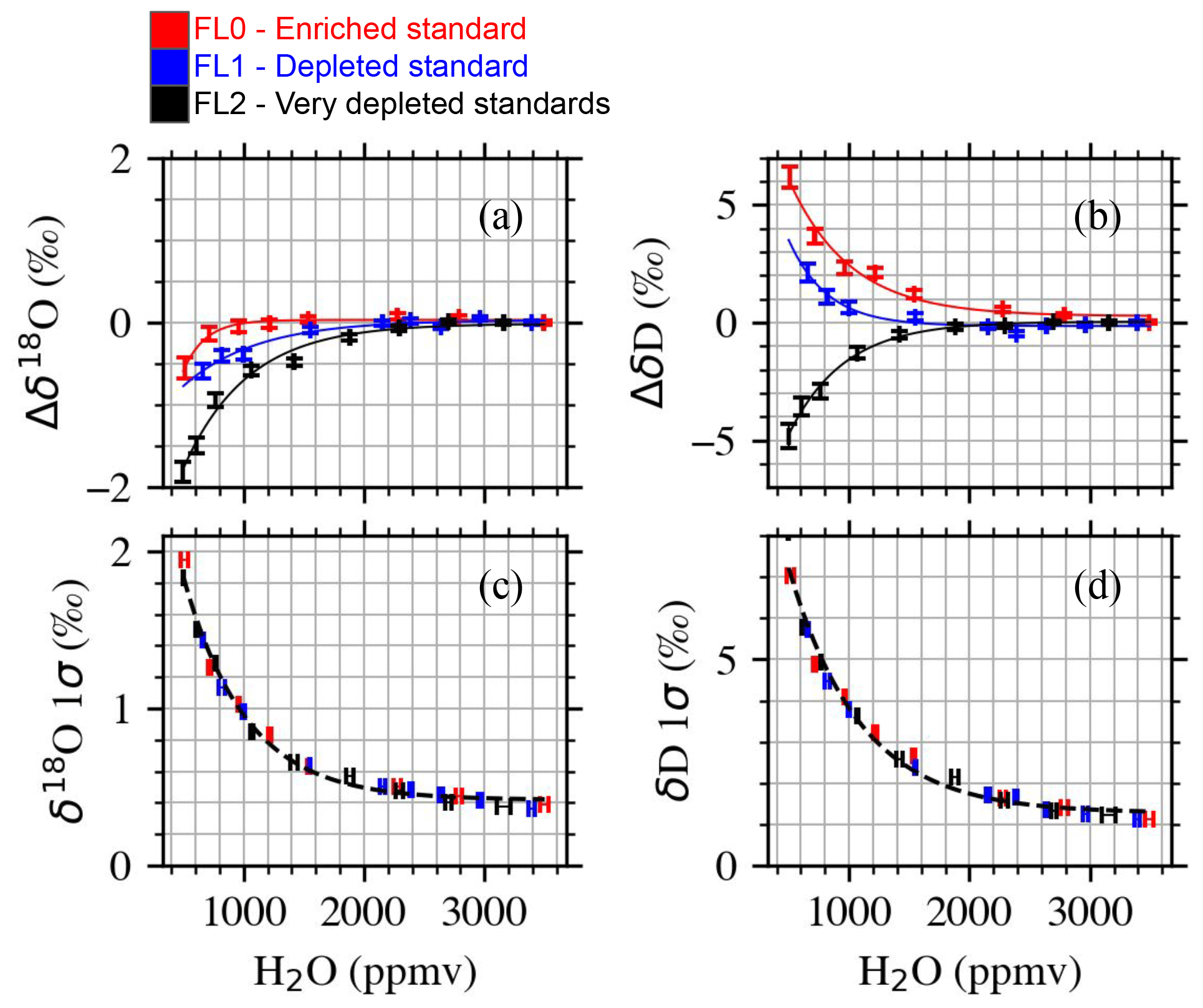
Figure 7 Humidity–isotope characterization of the HKDS2092 analyzer between 500 and 3500 ppmv using three different isotopic standards. (a, b) Humidity–isotope dependency for δ¹⁸O and δD, respectively. Dependency reported as the difference between the isotopic composition at 3500 ppmv and isotopic composition for each humidity step. Error bars are standard errors of the mean. Lines are exponential decay models that best fit the observations of each isotope standard. (c, d) Standard deviation of δ¹⁸O and δD for each humidity step and different standards. Error bars on the horizontal axis are standard deviations. For all panels, results of the best fits are reported in Table S5.

Interestingly, the CRDS analyzer showed slightly different patterns of δ¹⁸O for the different standards used, and a very different pattern is observed for δD for the very depleted standard as also reported earlier by Weng et al. (2020). Importantly, we note that the precision of the CRDS analyzer is not affected by the isotopic composition of the standards, as shown in Fig. 7c and d. Users of CRDS analyzers at very low humidity must be aware of the different humidity–isotope sensitivities for different isotopic composition, which might be due to issues with fitting of the spectra and could be instrument dependent.

3.5 Application study 2: Δ¹⁷O analysis of liquid samples

The two reference waters SW and WW, with known Δ¹⁷O values, were mixed in three different aliquots to obtain three solutions with known Δ¹⁷O of 20 mL each (see Table S2 for details on aliquots). The solutions of reference waters were weighted using a laboratory scale with 0.01 g resolution. Half of the maximum span obtained by mixing SW ± 0.01 g with WW ± 0.01 g yields a 13 per meg variation of the final Δ¹⁷O value, which can be considered a conservative estimate of the sample uncertainty due to weighing. A typical analysis run consisted of injecting the two standard waters (SW and WW) followed by injections of the two solutions (∼ 15 000 ppmv). Each injection lasted for 3 h, and a typical run consisted of 7–12 injections for a total time of approximately 21–36 h per run. For both reference waters and solutions, the first 2 h of each injection was discarded to limit the memory effect introduced by the injection of the previous sample. A linear calibration was performed by using reference SW and WW values for δ¹⁸O and δ¹⁷O. Since the standards were measured from 2 to 4 times for each measurement session and the solutions were measured on different days, we applied both an average and independent calibration. The average calibration factors for the former were estimated by averaging the raw observations of the standards injected for all the runs, while the independent calibration factors were calculated for each couple of reference standards and then applied only to the following couple of solutions (two standards followed by two samples). The results of the experiment are reported in Table 2.

Despite the fact that the analysis was performed on three different samples only, Table 2 clearly shows that the reproducibility of sample measurement is very high: 4 and 5 per meg on average for average and independent calibrations, respectively. Such reproducibility is comparable to the precision achieved with IRMS (e.g., Barkan and Luz, 2005; Steig et al., 2014) and to the total error obtained within the latest development in continuous-flow analysis of ice cores (Davidge et al., 2022), but it is better than the analysis performed with optimal settings of the vaporizer and autosampler from Picarro, which is 8 per meg following Schauer et al. (2016). The root mean squared error is 8 per meg, and in general the measured Δ¹⁷O is 5–6 per meg higher than the expected values but within the expected uncertainty due to the weighing uncertainty, which could produce an offset of up to 13 per meg. The memory effect was estimated to have a limited impact on Δ¹⁷O, as further discussed in Sect. 4.4, and we argue the systematic difference can be due to measurement error of the weighing scale, degraded quality of the reference waters due to long storage time, or biases in assigned Δ¹⁷O values of reference waters. Despite the small bias, this analysis represents a line of evidence suggesting that the calibration module can successfully be used to analyze Δ¹⁷O in liquid water given its ability to measure a sample for potentially an extended time.

4 Discussion

4.1 Drivers of measurement noise

To investigate the origin of the water isotope measurement noise, we placed two Picarro L2140 instruments (HKDS2092 and HKDS2156) in parallel in a configuration such that they measured the same output generated by the water vapor generator module at the 14 500 ppmv level for 10 h with the BER standard. A 1 m length, 3.125 mm o.d. copper tube coming from the water vapor generation module was connected to a stainless-steel tee (SS-200-3, Swagelok). Two nearly identical 0.75 m,​​​​​​​ 3.125 mm o.d. copper tube segments were connected to the tee, carrying the sample gas to each analyzer. The instrument connection at the gas inlet was reproduced as similarly as possible for both instruments to achieve the same gas transport resistance. Both instruments were connected to the inlet line in open-split mode, and each instrument was pulling the gas sample at its nominal flow rate (∼ 40 sccm). The water vapor generation module was configured to keep at least a flow rate of 100 sccm at its output to compensate for the requirements of two instruments measuring at the same time. The excess gas sample was released into the room air.

Table 2 Analysis of Δ¹⁷O of liquid samples using the vapor generation module. All Δ¹⁷O values are in per meg. Analytical precision is standard error multiplied by Student's t factor for a 95 % confidence limit.

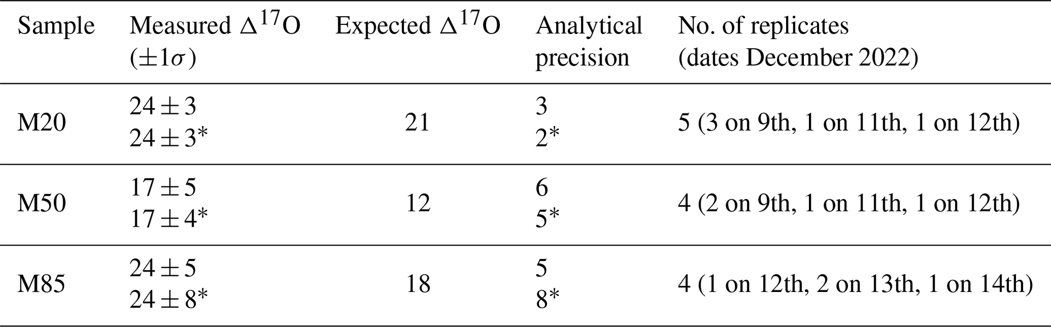
^* indicates independent calibrations for each run.

The newer HKDS2156 instrument is performing better than the HKDS2092 in terms of noise and precision, as shown in Fig. 8a. In the figure, bumps in the Allan deviation plot for both instruments are seen at different timings for different isotopes and with differences, which are instrument dependent. This supports the hypothesis that the main driver of the noise in δ¹⁷O, δ¹⁸O, and δD is related to the analyzers' characteristics and not to the vapor generation module. A simple correlation analysis of the synchronized and resampled (1 Hz) H₂O signal between the two analyzers yielded r = 0.91. An insignificant correlation (< 0.01) was observed for δ¹⁸O, showing that even though H₂O variability due to vapor generator fluctuations is captured by the two instruments, no co-varying isotopic composition change can be detected by the two instruments during the test (for completeness, δ¹⁷O and δD measured with the two analyzers have correlations < 0.01 and ∼ 0.01, respectively). Since the variability of the isotopic composition of the signal is independent of the mixing ratio variability, the main sources of isotope variability in the measurement must be investigated in the analyzer performances. The isotope data recorded at ∼ 1 Hz by both analyzers do not correlate with any of the following parameters recorded in the log file of the analyzer: cavity temperature, cavity pressure, internal computer temperature referenced as “DAS temperature”, or warm-box temperature. However, a wavelet analysis reveals significant power in periods with 10 to 60 min periodicity in δ¹⁸O and cavity temperature. When performing a wavelet coherence analysis (Grinsted et al., 2004), we find a significant in-phase coherence between δ¹⁸O and cavity temperature for periods in the range of 10 to 60 min for the HKDS2092 and in the range 10 to 30 min for the HKDS2156 instrument (see Fig. B2). When a low-pass Butterworth filter is applied to the data, as shown in Fig. 8b, we detect a significant correlation between δ¹⁸O and cavity temperature. For instance, a Butterworth low-pass filter with cutoff periods of less than 600 s yielded r=0.68 for HKDS2092 and r = 0.59 for HKDS2156. Correlations also increase for δ¹⁷O and δD but not as much as for δ¹⁸O (e.g., with the same time window, the correlation between δ¹⁷O and cavity temperature is only 0.31 for HKDS2156). It is important to note that the cavity temperature control is precisely tuned using a PID loop, and it is not accessible at the user level. We note that a similar bump can be seen in Allan deviation analyses presented in previous studies (e.g., Leroy-Dos Santos et al., 2021; Steig et al., 2014), and we hence speculate if the observed significant periodicity in cavity temperature in the range 12 to 30 min is consistent across instruments. Should this hypothesis be correct, it would imply that δ¹⁸O precision for measurements averaged between 10² and 10³ s could be improved by up to a factor of 2 if the PID-driven cavity-temperature cycles were to be dampened. We also further notice that this increase in Allan deviation occurs at similar integration times as used for liquid measurements, which makes it even more important to improve.

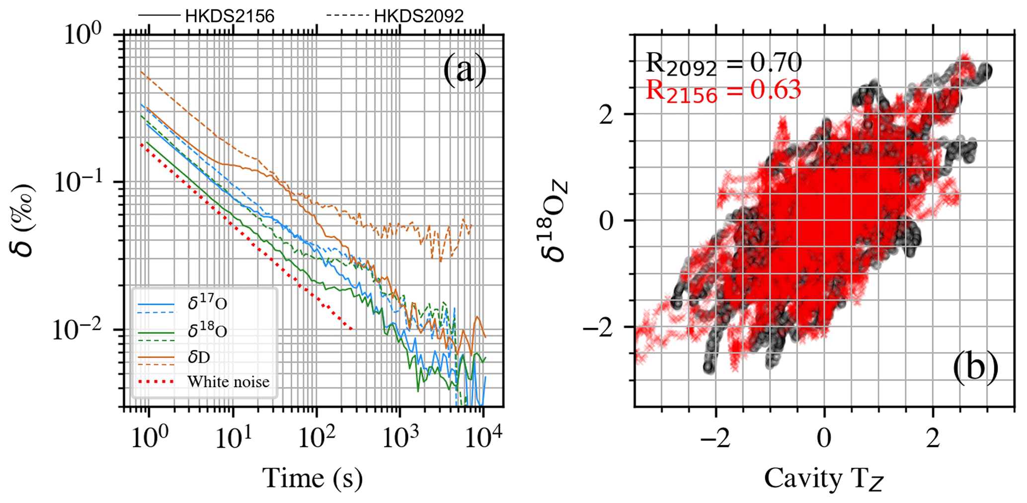
Figure 8 The 10 h analysis of the same water vapor source using two water isotope analyzers (HKDS2092, HKDS2156). (a) Allan deviations of the two analyzers showing bumps at different averaging times for the two instruments. The Allan deviation of white noise is reported as a dotted red line for reference. (b) z scores of δ¹⁸O vs. z scores of cavity temperature of the two instruments (HKDS2092 in black, HKDS2156 in red). Standard deviations of δ¹⁸O are 0.02 ‰ and 0.01 ‰ for HKDS2092 and HKDS2156, respectively. Standard deviations of cavity temperature are 0.002 and 0.001 K for HKDS2092 and HKDS2156, respectively.

4.2 Isotope calibration pulses

To test the repeatability of the calibration system for producing calibration cycles suitable for water vapor analysis, the standards BER and SP were used to autonomously produce 100 min pulse trains spaced every 3 h for 48 h continuously. The test was performed with the multiple oven configuration using two different lines to stream from the two different standard 2 mL vials. The mixing ratio level was kept constant at 10 000 ppmv in order to have enough water inside the vials to allow for repeated injections for 48 h. The isotopic composition variability of the injected water for each pulse centered around the mean, calculated as the average ±1 standard deviation of the last 5 min of the δ¹⁷O, δ¹⁸O, δD, d-excess and Δ¹⁷O signals, is reported in Fig. 9.

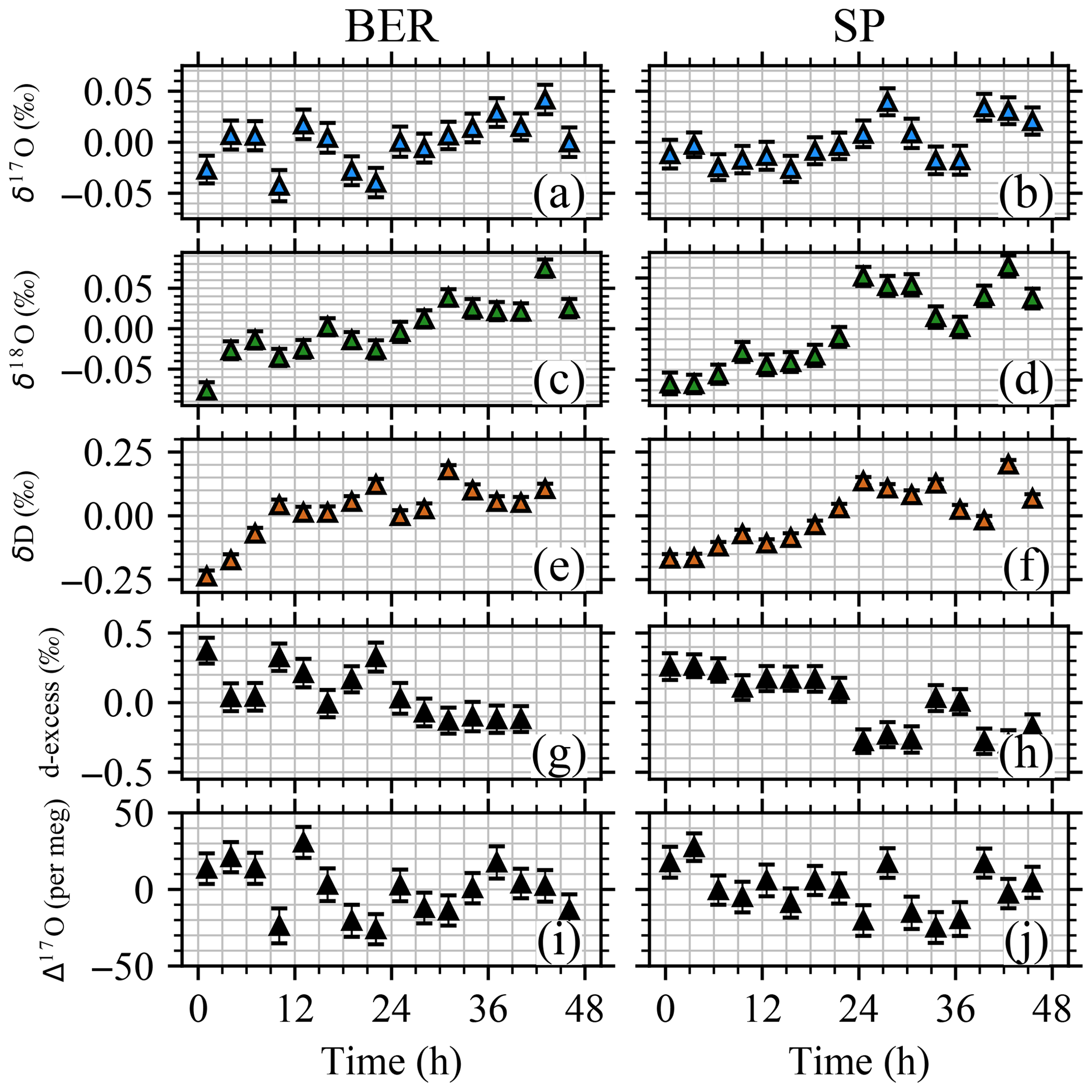
Figure 9 Variability of repeated injections of BER and SP standards using the multiple ovens configuration (raw data). Results reported as average ± standard error were calculated for the last 5 min of δ¹⁷O (a, b), δ¹⁸O (c, d), δD (e, f), d-excess (g, h), and Δ¹⁷O (i, j) signals. The results are centered around the mean value of all the injections to improve visualization.

The calibration system successfully injected both SP and BER standards autonomously, reporting no failed injections for 48 h. No large change in isotopic composition of the injected standards were observed for 48 h for the multiple oven configuration. However, as can be observed in Fig. 9, there appears to be slight enrichment in the two standards throughout the experiment as indicated by the decrease of the d-excess value (∼ −0.6 ‰ for both standards). This drift (increase in delta values) of the measurements could be a result of instrumental drift, but we understand the enrichment to be a result of the long exposure of the liquid sample to the dry push gas inside the vial, leading to evaporation and hence enrichment. The dry push gas from the headspace of the vial is being replaced after each injection when stopping the flow of water into the capillary. This observed drift means that whenever a sample in a vial will be measured for a continuously long period of time, it is important to use a relatively larger sample holder to limit the relative influence of evaporation. The variability in the mean of the last 5 min of the injection is relatively small, with standard errors ranging in the order of 0.01 ‰, 0.01 ‰, 0.02 ‰, 0.1 ‰, and 11 per meg for δ¹⁷O, δ¹⁸O, δD, d-excess, and Δ¹⁷O, respectively. To illustrate the repeatability of the injections, the standard deviation of the mean values from the individual pulses is 0.02 ‰, 0.02 ‰, 0.09 ‰ and 0.13 ‰ for δ¹⁷O, δ¹⁸O, δD, and d-excess, respectively, when linearly correcting for the long-term drift likely induced by evaporation. Δ¹⁷O shows no significant change with time, and the standard deviation of the mean values from the individual pulses is 16 per meg.

This experiment illustrates the potential of the system to be used as a calibration unit for atmospheric water vapor isotope measurements in the field. As we will discuss below, the most often occurring issue when using the vapor generation module was clogging of the capillary providing water to the flash evaporator oven. The operator of the system for field calibration of water vapor isotope measurements therefore needs to use relatively clean (such as Milli-Q water) standards to allow for extended operation. As illustrated in the long-term stability experiment in Fig. 3, we have carried out a successful ∼ 90 h long injection of a single standard. We have used the calibration system in the laboratory and during field campaigns for about 2 years now, and we found that a stable performance of the vapor generation module is dependent on using clean standards. When using in-house-generated standards consisting of a mixture of melted Greenland snow and Milli-Q water from Bermuda, we have successfully operated the vapor generation module daily (roughly 1–3 h d⁻¹) in the laboratory for more than 6 months without changing the capillaries.

4.3 Capillary issues

To control the flow of water into the oven as precisely as possible, it is beneficial to use a capillary with a small internal diameter between 50 and 350 µm. However, as a consequence of the flash evaporation at the tip of the capillary inside the oven, residue from dissolved and non-dissolved impurities in the water is building up, ultimately leading to clogging of the capillary. Typical signs of clogging are a gradual decrease in humidity and enhanced variability in the humidity, which occur within a few days of operation when using non-clean standards. Following Gkinis et al. (2011), we started out using a silica capillary but discovered that using a stainless-steel capillary (T10C5, VICI) resulted in enhanced performance in terms of length of operation before signs of clogging appeared. We also observed that using a stainless-steel capillary had the advantage that it could be placed the same way every time, while the capillary would touch the nut of the oven due to the flexibility of the silica capillary, leading to a non-uniform heating at the tip. Such cases of non-uniform heating were often seen as increased variability in the generated humidity. We do not have an explanation for why the stainless-steel capillary was performing better. From experience, we observed that using a capillary with an i.d. of 127 µm created the overall best performance. Once a capillary was clogged, we had partial success to unclog it by placing it in an ultrasonic bath with deionized water. We were able to extend the lifetime of the clogged capillaries by cutting the last 2 cm off. As we will discuss in detail below, the clogging of the capillary had consequences for changing the memory effect. While our experience using our in-house clean standards shows stable performance by the vapor generation module, we have also used standards which were provided to us by other labs. In those cases, we observed that the capillary would get clogged more frequently and had to be replaced every 2–4 weeks. To extend the lifetime of the capillaries, it is possible to use a larger i.d., but this can potentially result in less-stable humidity values.

4.4 Memory effect

As documented in Sect. 3.2, memory effects need to be considered when using the vapor generation module for measurements of samples with a large spread in water isotopic composition. The vapor generation module shows an approximate factor of 4 reduction in the memory effect for δD compared to liquid injections using an autosampler and vaporizer. However, in the work mode applied here, the control software will automatically adjust the dry air dilution to maintain a targeted humidity set point. The consequence of this is that during a build-up of non-dissolved impurities, less water will be delivered at the tip of the capillary, and the control software will reduce the flow of dry air. Less water and air molecules will therefore flow through the system, leading to a reduction in removal of water molecules from the previous sample. An example of such a situation is illustrated in Fig. S4 for a similar pulse train of standard injections as discussed in Sect. 4.2 with an approximate jump of 55 ‰ and 435 ‰ in δ¹⁸O and δD, respectively, obtained by injecting the BER and SP standards. We do not know of similar published tests with other types of vapor generation modules, but we expect that a similar variability in the memory effect must also be present for other modules. Our presented example therefore stands as a lesson in the need for quantifying and tracking the performance of every aspect when measuring standards and unknown samples. When using the vapor generation module in automatic measurement mode, one must therefore characterize the memory effect of the setup as a function of dilution flow rate and have the control system log the flow rate for post-memory-effect correction of the sample and standard measurement.

The difference in the memory effect for the individual isotopes as documented in Fig. 4 illustrates the need to reject relatively longer measurement times to obtain accurate δD measurements compared to δ¹⁸O. We speculate that the difference in the memory effect between δD and δ¹⁸O originates from the difference in polarity of the HD¹⁶O and ${{\mathrm{H}}_{\mathrm{2}}}^{\mathrm{18}}\mathrm{O}$ molecules, with the HD¹⁶O adhering relatively strongly to the sides of the tubing. This difference in the memory effect of δ¹⁸O compared to δD is not only important for obtaining the most accurate isotope values, but also means that care needs to be taken when calculating the d-excess. Interestingly, the memory effects for δ¹⁸O and δ¹⁷O are nearly identical (e.g., τ₉₅ = 335 and 333 s for δ¹⁸O and δ¹⁷O, respectively). Due to the relatively high measurement uncertainty (e.g., σ_Allan = 9 per meg at 15 min) and relatively small changes in Δ¹⁷O observed in natural waters (∼ 90 per meg), it is not the memory effect which is the limiting factor influencing the Δ¹⁷O measurements. As documented in Fig. 10, showing the memory effect for a Δ¹⁷O step change of approximately 90 per meg, already within the first hour of measurements, the memory effect is producing an error that is approximately 5 times smaller than the analytical error. Hence, the vapor generation module is highly capable of Δ¹⁷O measurements, as it can provide integration times over multiple hours for both standards and samples, allowing optimal treatment of memory effects and measurement noise to be reduced to a minimum.

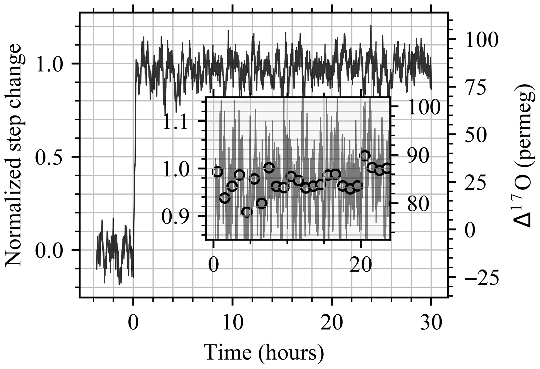
Figure 10 Calibrated and normalized step change for Δ¹⁷O. The black line is a 15 min moving-window average. Inset plot: detail of the 0–24 h region. Gray line is the same as in the main plot. Circles are 1 h averaged sample mean.

4.5 Potential future updates

We developed the vapor generation module system with four ovens, allowing four individual vials to be measured without interference from an operator. However, by connecting one of the ovens to a 10-port selector valve, we were able to run the system for liquid measurements using 3 known standards and 10 unknown samples. We are now in the process of setting up the system for a daily standard operating procedure measuring Δ¹⁷O of ice core samples. To increase further throughput by reducing the memory effect, one could also configure the N-oven system to initiate the vapor generation of the subsequent vial while the previous vial is being measured. It would then be a matter of simply switching to an already existing vapor stream from the next oven in line. We invite readers who plan to build a similar module to contact us for the latest update on measurement procedure and control software.

5 Conclusion

The water vapor generation module presented here represents a standalone modular system for water vapor isotope calibrations in the field and high-precision liquid water isotope measurements in the laboratory. The system is completely scalable from one sample/standard vial up to N vials. The vapor generation module is designed to be connected directly with a water vapor isotope analyzer without the need for additional auxiliary systems. There are several advantages of the system compared to existing systems for vapor calibration and liquid sample measurements for water stable isotopes, most notably the possibility of calibrating using several standards, the high dynamic range of humidity generation, the significant reduction in memory effect, and the possibility to (in principle) measure the same sample indefinitely.

We have used the vapor generation module to characterize the performance of two water isotope analyzers, and we documented that a key driver of the measurement noise for averaging times between 10 min and 1 h is driven by temperature fluctuations of the optical cavity inside the analyzer. This result provides guidance on optimal measurement integration times as well as points to the need for stabilizing the cavity temperature on these timescales. We argue that previously published increases in Allan deviation for longer averaging times could be a result of memory effects and not only driven by instrumental drifts as is often interpreted. We document Allan deviations of the water vapor isotope analyzer, yielding 0.004 ‰, 0.005 ‰, 0.01 ‰, and 0.04 ‰ σ_Allan for 10⁴ s averaging time for δ¹⁷O, δ¹⁸O, δD, and d-excess, respectively, as well as 2 per meg σ_Allan for 10⁴ s averaging time for Δ¹⁷O.

Despite the memory effect of the vapor generation module being, respectively, 2 and 3 times smaller compared to injections using an autosampler for δ¹⁸O, δ¹⁷O and δD, it is still possible to detect the memory effect after more than ∼ 20 h, thanks to the high measurement precision for the instrument. This result indicates that for achieving measurements with very low uncertainty as, for example, needed for ice core analysis of million-year-old ice, dedicated efforts on developing measurement systems with a minimal memory effect is needed. We find, however, that measurements of Δ¹⁷O are limited by the integration time of the vapor measurements and, to a lesser extend, the memory effect. By measuring an unknown liquid sample for Δ¹⁷O for a 3 h period (rejecting the first 2 h due to the memory effect), we document an average standard deviation of 4 per meg for Δ¹⁷O and an average standard error (95 % confidence limit) of 5 per meg.

We hypothesized that the measurement uncertainty using laser spectroscopy instruments would increase for more depleted values due to the lower number of heavy water isotopologues. Using standards spanning 55 ‰ and 435 ‰ in δ¹⁸O and δD, respectively, we do not find any evidence that measuring more depleted values results in higher uncertainty.

Using sufficiently clean water, we have been able to continuously measure a constant vapor stream from a single standard over a period of more than 90 h. This documents the feasibility of using the vapor generation module as an autonomous field calibration system. The PID control system, ensuring stable humidity levels along with the large range of possible humidity levels, makes the vapor generation module truly versatile, both in the field and in the laboratory.

Appendix A: Stability at different humidity levels

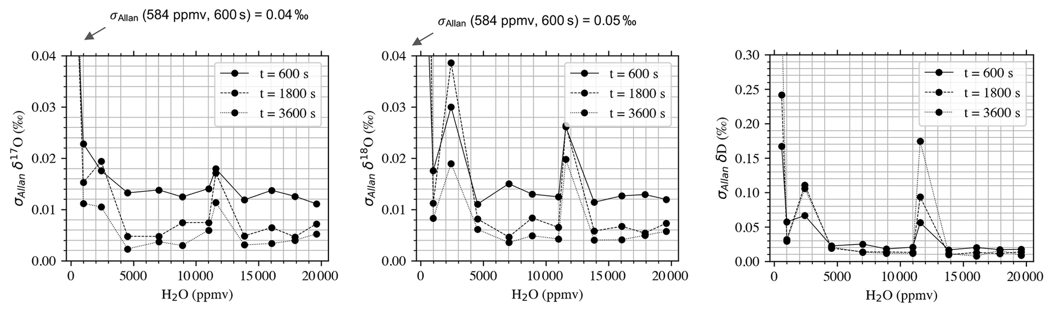
Figure A1 Allan deviations for δ¹⁷O, δ¹⁸O, and δD at 600, 1800, and 3500 s integration times as a function of humidity level.

Appendix B: Squared wavelet coherence analysis between δ¹⁸O and cavity temperature

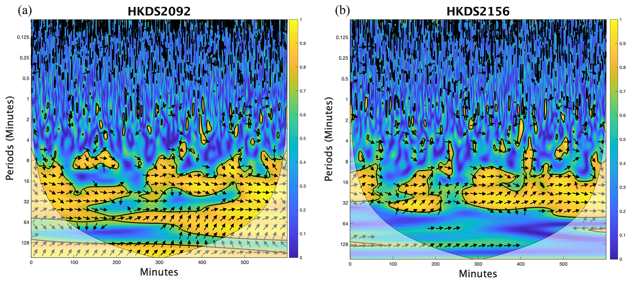
Figure B1 Squared wavelet coherence analysis between the measured δ¹⁸O and recorded cavity temperature of the two Picarro analyzers (a) HKDS2091 and (b) HKDS2156 using the procedure by Grinsted et al. (2004). The 5 % significance level against red noise is shown as a thick contour. Arrows indicate phasing (angle corresponds to phase behavior). In-phase behavior of δ¹⁸O and recorded cavity temperature are observed for periods between ∼ 12 and ∼ 30 to 60 min for, respectively, the HKDS2156 and HKDS2092 analyzers.