the Creative Commons Attribution 4.0 License.
the Creative Commons Attribution 4.0 License.
 | 23 Jan 2024
Real-time pollen identification using holographic imaging and fluorescence measurements
Sophie Erb
Elias Graf
Yanick Zeder
Simone Lionetti
Alexis Berne
Bernard Clot
Gian Lieberherr
Fiona Tummon
Pascal Wullschleger
Benoît Crouzy
Over the past few years, a diverse range of automatic real-time instruments has been developed to respond to the needs of end users in terms of information about atmospheric bioaerosols. One of them, the SwisensPoleno Jupiter, is an airflow cytometer used for operational automatic bioaerosol monitoring. The instrument records holographic images and fluorescence information for single aerosol particles, which can be used for identification of several aerosol types, in particular different pollen taxa. To improve the pollen identification algorithm applied to the SwisensPoleno Jupiter and currently based only on the holography data, we explore the impact of merging fluorescence spectra measurements with holographic images. We demonstrate, using measurements of aerosolised pollen, that combining information from these two sources results in a considerable improvement in the classification performance compared to using only a single source (balanced accuracy of 0.992 vs. 0.968 and 0.878). This increase in performance can be ascribed to the fact that often classes which are difficult to resolve using holography alone can be well identified using fluorescence and vice versa. We also present a detailed statistical analysis of the features of the pollen grains that are measured and provide a robust, physically based insight into the algorithm's identification process. The results are expected to have a direct impact on operational pollen identification models, particularly improving the recognition of taxa responsible for respiratory allergies.
- Article
(3535 KB) - Full-text XML
- BibTeX
- EndNote


Over the past decades a considerable increase in aeroallergen-related diseases such as asthma or allergic rhinitis has been observed (Ring et al., 2001; Woolcock et al., 2001; Woolcock et Peat, 2007). This has resulted in a rise in associated direct and indirect health costs in terms of hospitalisation, medication costs, and absence from work (Zuberbier et al., 2014; Greiner et al., 2011). Currently, the prevalence of pollen allergies ranges between 10 % to 30 % of the population in westernised countries and up to 40 % of children in high-income countries (Pawankar et al., 2011). In future, the relevance of pollen as an allergen may increase further as a result of climate change, which perturbs the life cycle of plants through drier environmental conditions and increased temperatures. Stressed plants tend to have an earlier and/or longer blooming season (Ziello et al., 2012) and produce more pollen with higher concentrations of allergens (Damialis et al., 2019; Beggs, 2016; D'Amato et al., 2016), possibly further contributing to the increase and severity of allergic diseases. For these reasons, systems to measure airborne pollen concentrations are essential to meet public health challenges associated with respiratory allergies. Through real-time measurements and the development of forecast models (Chappuis et al., 2020), they can help reduce health costs with better diagnosis and prevention, thus helping patients to better manage their symptoms.
Most European countries started monitoring pollen in the second half of the 20th century using Hirst-type instruments (Hirst, 1952) with manual identification and counting part of the process (Clot, 2003; Spieksma, 1990). However, this method provides data at low time resolution, typically daily mean values, after a processing time of up to 10 d. The spread of pollen grains on the collection band and the limited sampling (Oteros et al., 2017) mean that data at higher temporal resolutions or at low concentrations (below 10 pollen grains m−3) have considerably increased uncertainty (Adamov et al., 2021). Although few data are available to study atmospheric pollen phenomena at high temporal resolutions, it is widely expected that pollen production and dispersal processes take place at sub-daily scales since they are highly influenced by local meteorological environmental conditions (Rojo et al., 2015; Rantio-Lehtimäki, 1994). Provision of real-time pollen data is also crucial for forecasting purposes, since models can then integrate these real-time data to deliver considerably improved forecasts (Sofiev, 2019).
Over the past few years, several instruments designed for real-time pollen monitoring have come onto the market (Crouzy et al., 2016; Oteros et al., 2015), as comprehensively reviewed in previous work (Huffman et al., 2020; Buters et al., 2022; Maya-Manzano et al., 2023). Among the most promising instruments are airflow cytometers, which allow the characterisation of particles almost in real time as they pass through the instrument and enable continuous monitoring with high temporal resolution (10 min as for weather parameters or below) over a whole season. In particular, the SwisensPoleno Jupiter (developed by Swisens AG, Switzerland) is an instrument for bioaerosol identification which can take in-flight holographic images of particles and measure their fluorescence (FL hereafter) (Sauvageat et al., 2020; Tummon et al., 2021; Lieberherr et al., 2021). Coupled with a machine learning (ML) algorithm, it has been shown to perform well for pollen monitoring even if the algorithm uses just the holographic data (Sauvageat et al., 2020; Crouzy et al., 2022; Maya-Manzano et al., 2023).
The FL data have to date not been used for pollen identification with the SwisensPoleno Jupiter. Sauvageat et al. (2020) reached an accuracy above 96 % for eight of the main allergenic pollen species in central Europe (Ambrosia artemisiifolia, Corylus avellana, Dactylis glomerata, Fagus sylvatica, Fraxinus excelsior, Pinus sylvestris, Quercus robur, and Urtica dioica) using only holographic images. However, some species have similar morphologies, which can cause misclassifications and thus lower the algorithm performance, as previously identified in Sauvageat et al. (2020). In this paper, we investigate whether FL helps discriminate single pollen grains between different allergenic taxa based on their chemical compositions to reduce the level of confusion resulting from their similar shapes. Moreover, we also verify whether the FL measurements are consistent for each species when using different SwisensPoleno units.
In this work we investigate the impact of including the set of FL measurements, constituting the particle FL spectra, as input for pollen identification using artificial neural networks. We trained and assessed the performance of three neural networks with the same dataset but using different inputs: only holographic images (holo), only FL spectra (FL), or both (combined). The performance of each model is evaluated using classical metrics, here the balanced accuracy, the F1 score, and Matthew's correlation coefficient (MCC) as defined in Chicco et al. (2020), as well as the (relative) error rate derived from the accuracy.
2.1 Pollen holography and fluorescence dataset
The SwisensPoleno Jupiter measures particles in flight, in the size range from 0.5 to 300 µm, as they pass through the instrument. When a particle triggers the detector, holographic images are taken by two cameras, which are both orthogonal to the direction of flight and at 90∘ to each other. These images are greyscale with a resolution of 200 by 200 pixels after numerical reconstruction and cropping, with each pixel representing a square of 0.595 × 0.595 µm in the physical domain. Right after the holographic images, FL is measured using the laser-induced fluorescence (LIF) method. FL is then sequentially induced by three excitation sources and captured in five different wavelength channels, for a total of 15 measured FL intensities. For each source, the FL is induced by shooting at the particle at the moment it passes the detector, and the FL subsequently emitted by the particle is captured by silicon photomultipliers (SiPMs). The FL lifetime is also measured but is not used in the present work. The three different excitation wavelengths are 280, 365, and 405 nm, while the reception wavebands are 333–381, 411–459, 465–501, 539–585, and 658–694 nm. In the following, we refer to each waveband by its central wavelength, i.e. 357, 435, 483, 562, and 676 nm. Note that the first measurement channel is saturated by scattered light when the 365 nm excitation source is activated. Also, for single-photon excitation, we expect to measure no signal in the first measurement channel when the 405 nm source is active. This effectively reduces the useful intensity measurements to 13. The FL data require additional pre-processing to simplify their usability and improve robustness. More details on these steps are provided in Sect. 2.2. Finally, the SwisensPoleno Jupiter also performs polarised-scattered-light measurements, which are however not used in the present work. We therefore limit the analysis to characterisation of particle morphology using digital holography and chemical composition with FL intensity measurements. From hereon, we refer to the set of holographic images and FL measurements for each individual particle as “an event”. A more extensive description of the data collection process is provided in Sauvageat et al. (2020).
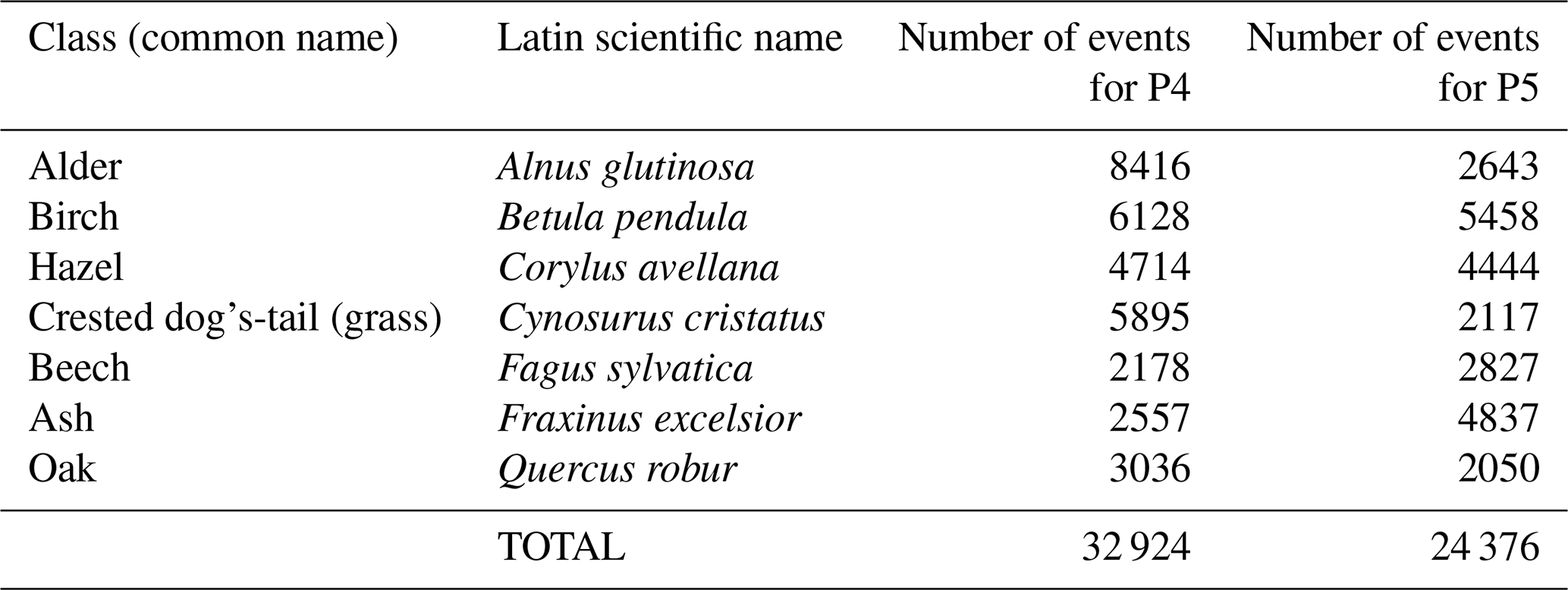
This study is based on a pollen dataset created by aerosolising freshly collected pollen at the Swiss Federal Office of Meteorology and Climatology MeteoSwiss (hereafter MeteoSwiss) station in Payerne, Switzerland. In total, the dataset consists of measurements from 57 300 pollen grains distributed among 7 different wind-pollinated and allergy-relevant plant taxa, as reported in Table 1. For simplicity, we also refer to these taxa as “classes”, and only the genus name is used to refer to each of them. In Fig. 1, we present examples of reconstructed images for the different classes considered in this work. To compare results across different instruments (of the same type), all measurements were performed using two SwisensPoleno Jupiter systems denoted, P4 and P5. The counts for each pollen taxon and SwisensPoleno are also given in Table 1.
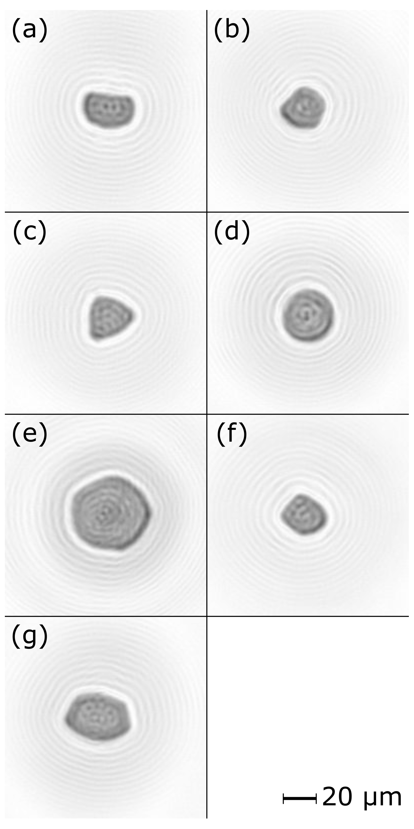
Figure 1Holographic images of pollen after numerical reconstruction: (a) Alnus glutinosa, (b) Betula pendula, (c) Corylus avellana, (d) Cynosurus cristatus, (e) Fagus sylvatica, (f) Fraxinus excelsior, (g) Quercus robur.
The pollen samples were collected from a single tree for Alnus, Betula, Corylus, Fagus, and Quercus; from two different trees for Fraxinus; and from a few neighbouring stems for the grass Cynosurus. After collection, pollen was brought to the outdoor measurement site and aerosolised. This was achieved using a SwisensAtomizer, which disperses particles using a vibrating membrane and an airstream. Samples are thus scattered in a chamber and drawn into the instrument, producing a regular flow of pollen grains. To prevent the pollen from drying out, plants that were not more than 15 km away from the MeteoSwiss station were selected, which means it was possible to aerosolise samples soon after collection (usually within 1 h). Pollen samples were analysed using two instruments one after another, implying a time lag between the data for P4 and P5, which ranges from just 35 min for Alnus to 80 min for Quercus (the mean time lag is 60 min). For Fraxinus there is no such lag since the data come from two different samples that were measured on different days. Datasets for all the considered pollen taxa were created in 2020, except Alnus and Corylus, which are from early 2021.
Table 1Distribution of pollen counts per taxon and SwisensPoleno.
2.2 Data pre-processing
The datasets required to train the algorithms were generated as follows. First, the holographic data for each class were cleaned to eliminate any non-pollen events or events associated with other pollen taxa. This was achieved with additional filters on shape properties (image features computed after binarisation as described in Sauvageat et al., 2020), which were appropriately selected for every class by heuristic visual inspection of the holographic images. Thereafter, for each event the background signal caused by scattered light was subtracted from the raw FL measurement. This background especially disturbs the low-FL-intensity measurements where the scattered light dominates relative to the particle signal. The background signal was obtained by conducting measurements with no particles present in the measurement chamber, leaving just the scattered light induced by the excitation source. If the subtraction caused the final signal to be negative due to noise, the resulting value was set to zero to avoid numerical instabilities that our ML model would not be able to deal with. Finally, since the absolute FL compensated by the scattered light is still dependent on the measuring system, the particle size, and the particle position within the measurement volume, we transformed it into relative FL. Namely, the relative fluorescence intensity rij for measurement channel i and excitation source j is obtained by dividing the absolute FL intensity aij by the sum of the FL intensities on all channels k for the same excitation source j:
Using relative FL, although we lose the absolute FL intensities, allows measurement systems to be compared without specific data modification. The inter-compatibility aspect is especially important when considering a measurement network. Thanks to this standardisation, the same algorithm can be used for all systems in the network rather than adjusting the classification algorithm individually for each measurement system.
2.3 Data exploration
Before applying any ML algorithm, it is important to explore the data to better understand their characteristics. In the following, the distributions of the various holographic image features as well as typical relative FL spectra for the different pollen types are investigated. We also explore the structure of the data using dimension reduction.
To get other characteristic features from the reconstructed holographic images, further image processing steps are conducted using the Python package “scikit-image” (Van der Walt et al., 2014). Physically based particle features, such as the minor and major axes, the area, the eccentricity, and the particle brightness (mean intensity of the pixels reproducing the particle), are computed for each image separately. Other statistics were calculated based on image features, e.g. the equivalent area diameter defined as the diameter of a circle with the same area as the particle. The distributions of these features for each pollen class and each measurement system were analysed separately and are presented in the Results section.
As previously discussed, alongside the holography images, relative FL spectra are used for enhanced characterisation of the pollen grains. During data exploration, we observed inconsistent results for the 405 nm laser excitation, which upon further inspection revealed a misalignment of this laser in one of the measurement systems. For this reason, we only use the 280 and 365 nm excitation throughout the rest of the present work. The distributions of the valid FL spectra are presented and discussed in the Results section.
As a way to explore all the features of the dataset at once, we performed dimensionality reduction. We used the Uniform Manifold Approximation and Projection (McInnes et al., 2018), called UMAP, on the input data of each model (holo, FL, and combined). This technique allows us to plot multidimensional data as points on a plane; therefore it gives an insight on how similar/different data points are depending on how far from another they are in the plane.
2.4 Machine learning model
To handle the classification task, we randomly split the data into training (75 %) and test (25 %) sets and chose a multi-layer “deep” artificial neural network to learn how to identify pollen grains based on the training set. This network maps input data from the holographic images and relative FL spectra to the different pollen classes. The full network, built using the ML framework Keras (Chollet et al., 2015), is shown in Fig. 2. To handle the image input, an EfficientNet B0 model pre-trained on ImageNet is used (Tan and Le, 2019). It achieves state-of-the-art performance for classification tasks. For treating the spectral information, a single fully connected (denoted FC hereafter) hidden layer with 255 neurons is used. As a pre-trained model, the parameters of EfficientNet B0 are frozen and therefore not modified in the training on the pollen dataset. However, the parameters of the layers after it are optimised according to the training data. The results of the two feature extraction networks are concatenated, then dropout is added, and finally the result is passed to the decision layer. The width of this FC decision layer matches the number of classes (seven in this case). Lastly, the output is normalised by a softmax layer to obtain a probability distribution. To compute the loss, we used the cross-entropy function between the predicted and reference classes. To ensure a fair comparison, each model was trained for exactly 200 epochs. In training runs where only images or only relative FL spectra were used, the path not used was removed from the model graph (Fig. 2). The figure shows the model with both features active.
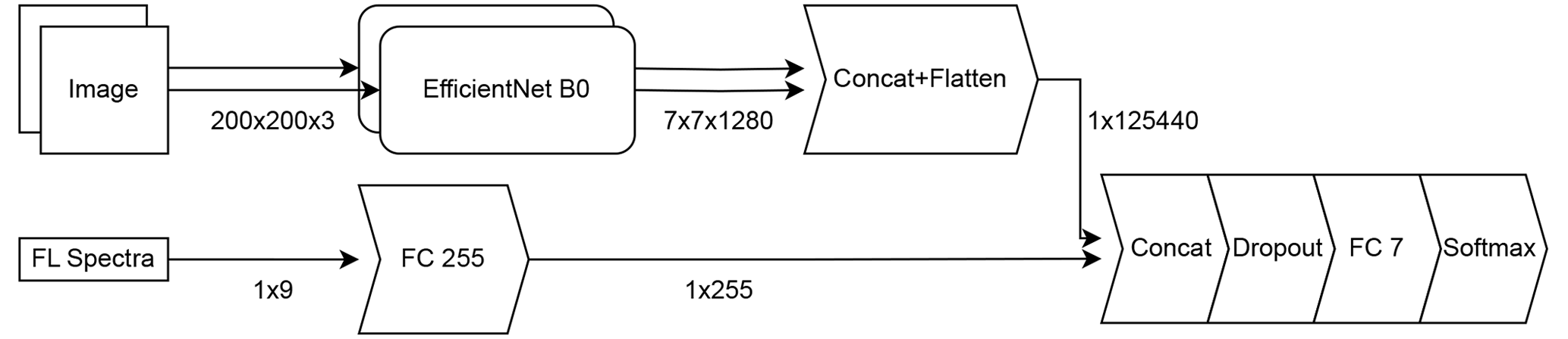
Figure 2ML model structure used to classify the pollen data. The top path handles the holographic image data, while the bottom path processes the relative FL spectra data. The numbers on the connecting lines denote the dimensions of the data.
The models were evaluated using a test set consisting of 25 % of the data from both instruments, sampled randomly. We used balanced accuracy, F1 score, and Matthew's correlation coefficient (MCC) as metrics to assess the model performance. For accuracy, the corresponding confidence intervals were calculated via normal approximation, as explained in Raschka (2020). It is important to note that the model used here is a baseline and has not undergone hyper-parameter optimisation; therefore no validation set has been defined in order to keep a maximum of data for training. This means that a degradation of scores is possible when applying the model to operational data as all sorts of pollen taxa can be encountered considering that other particles are filtered out before the classification. Nonetheless, the present study does not aim to provide an operational model but simply to investigate the potential of using FL as a complement to holography for single-particle identification.
3.1 Feature observations
Important observations can already be made by looking at basic geometrical features derived from holographic images. As an example, we consider the distributions of equivalent area diameter and eccentricity in Fig. 3a and b. Note that for geometrical features, the value associated with each particle is the largest result obtained for the pair of holographic images. Regarding the equivalent area diameter, its distribution provides information about the size of the pollen grains for a given class. As illustrated in Fig. 3a, Fagus pollen grains are typically large, with a maximum equivalent area diameter of 45–55 µm, which corresponds to the literature (Halbritter et al., 2021) and is clearly larger than all other classes we considered in our study. Conversely, the distribution of the eccentricity gives an insight on how round the pollen grains are. In that case, Cynosurus pollen grains have the roundest shape, with a maximal eccentricity between 0.4 and 0.55 (0 representing a circle and 1 an ellipse), whereas Quercus' values are in the range 0.8–0.9 due to its more elliptical shape. These characteristics can also be observed on the holographic images in Fig. 1. While the eccentricity is used to give a hint of the symmetry of the pollen grain, further metrics could be introduced to further quantify symmetry. This was not implemented in the present study as feature extraction is done automatically by the convolutional neural network.
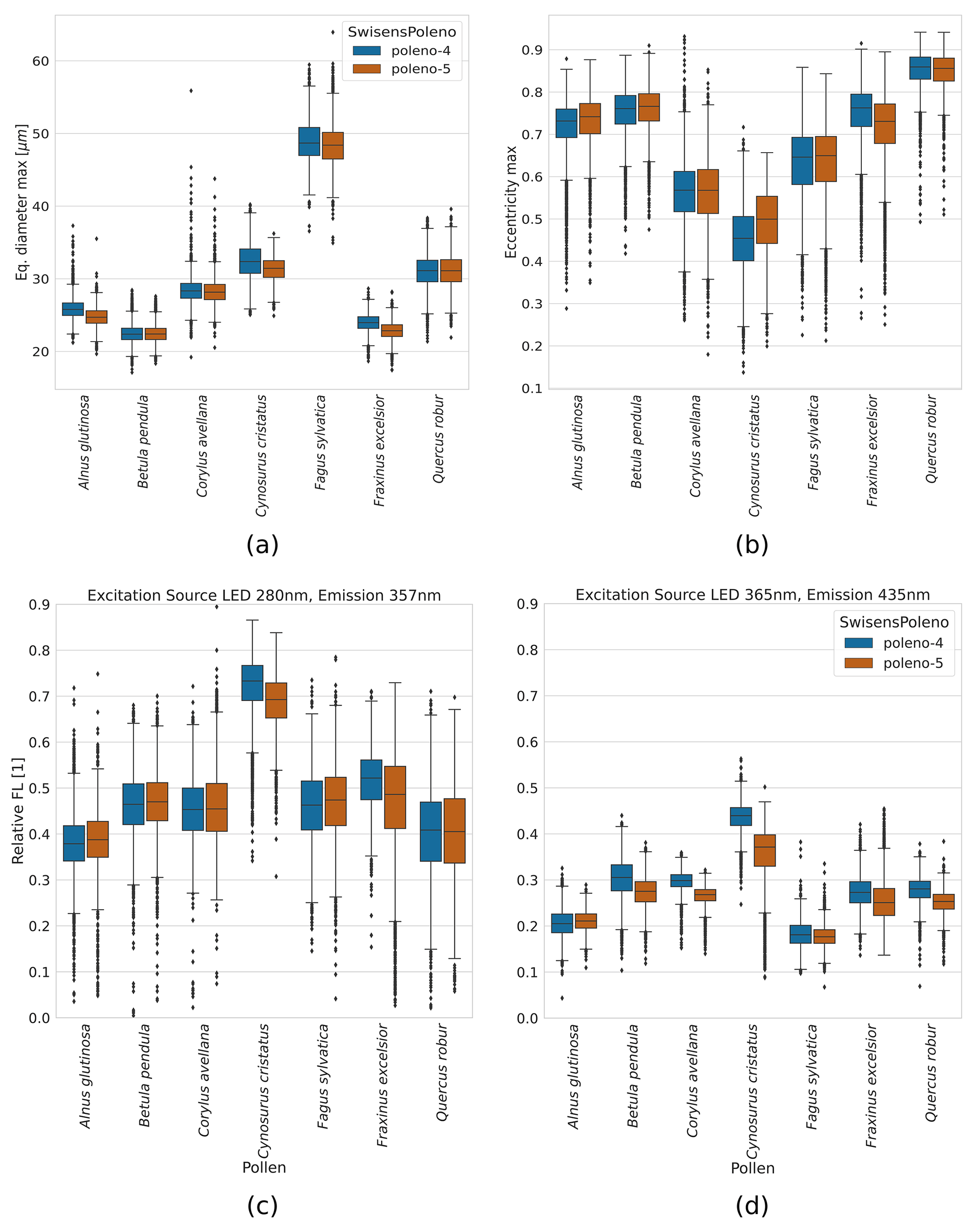
Figure 3Distribution of holographic image features (a, b) and relative FL (c, d) for each pollen class and measurement system. (a) Maximum equivalent area diameter in micrometres, defined as the diameter of a circle with the same area as the particle. (b) Maximum eccentricity, defined as the deviation of the ellipse fitted to the particle from a perfect circle, ranging from 0 for a circle to close to 1 for an ellipse. (c) Measured relative FL intensity with 280 nm excitation source and detector with a centre wavelength of 357 nm and (d) with 365 nm excitation source and detector with a centre wavelength of 562 nm.
The distributions of the relative FL spectra allow us to identify some classes that have distinct FL signatures. Figure 3c and d show the distribution of the relative FL for the two excitation–emission combinations where the differences between taxa are the largest. The excitation sources are at 280 and 365 nm, with emission channels at 357 and 435 nm respectively. In Fig. 3, we observe, for both plot c and d, clear differences in relative FL for Cynosurus, which presents considerably higher values compared to the other taxa. In addition, differences between instruments show that P4 and P5 have similar measurements at 280/357 nm, but P5 has significantly lower measurements for Corylus and Cynosurus at 365/435 nm. Overall, all combinations of excitation sources and emission channels provide relevant information for pollen characterisation, and the ones presented in Fig. 3c and d represent the type of patterns that can be observed well.
Finally, the UMAP plots, given in the left column of Fig. 4, show how different or similar the image and FL features of each taxon are. We observe a clear distinction based on morphology (Fig. 4a) for Fagus and Quercus, with Cynosurus also having only little overlap with Corylus. However, the latter and especially Betula and Alnus are clearly mixed up. In Fig. 4b, the UMAP on FL spectra does not exhibit the same group structure as for morphology. Here, Fagus and Cynosurus are plainly detached from the remaining groups, which are themselves imbricated. Ultimately, all groups are fully separated when building the UMAP on both morphology and FL features. We observe a correspondence between the separation of groups on the UMAPs and the capacity of the ML model to classify those classes correctly.
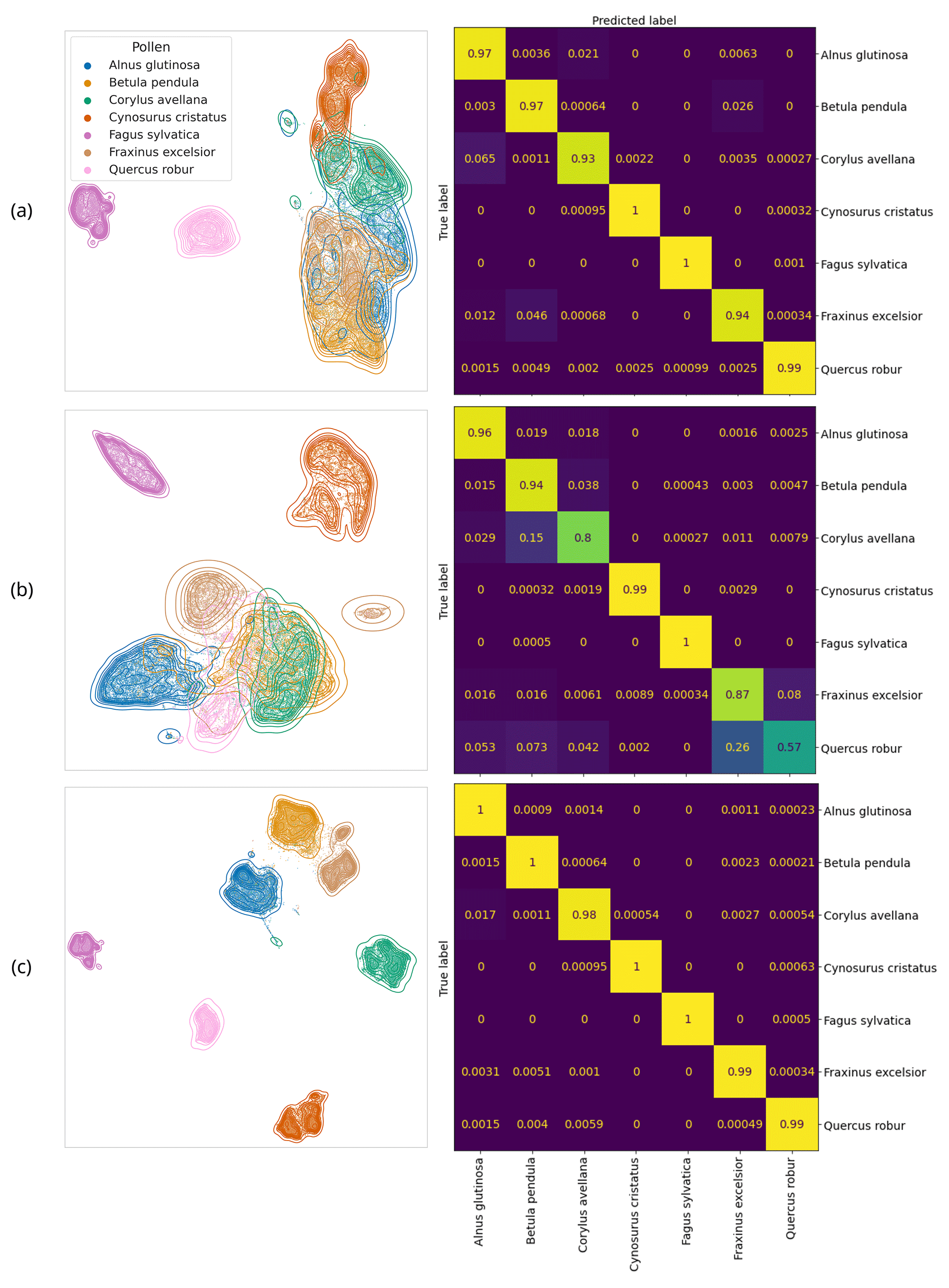
Figure 4Left side: Uniform Manifold Approximation and Projection (UMAP) of particle features (morphology or/and FL features) of all the data. Right side: confusion matrices indicating the performance of each model on the test set. (a) Holography only, (b) relative FL only, (c) combined relative FL and holography. UMAP settings: neighbours = 15, minimum distance = 0.001, random state = 42.
3.2 Classification performance
The classification results for each model are given as confusion matrices in Fig. 4 and summarised in Table 2. We observe in these results that the holo model globally performs better than the FL model when training on a single modality. The FL model indeed encounters difficulties distinguishing some classes such as Quercus and Fraxinus or Betula and Corylus (Fig. 4b), which exhibit similar relative FL spectra. When considering the morphology of Quercus and Fraxinus (Fig. 3a and b), it is not surprising that the holography model performs better at differentiating these classes as they present significantly distinct shapes. As the performance for the single-input models here is already (very) high, minor dips in performance can make a notable difference. Combining holography and FL improves the performance compared to the single-input models for every taxon considered, except for Fagus and Cynosurus, which already obtain perfect scores with single-input models. The performance gain is noteworthy as the combined model achieves an overall balanced accuracy of 99.2 % compared to either 96.8 % or 87.8 % for the individual holography or FL models respectively. As a complement, the confidence intervals associated with the accuracy of each model for each taxon are displayed in Fig. 5. The non-overlapping of the confidence intervals indicates a statistical difference between accuracies. The combined model outperforms both single-input models for five of the seven taxa, namely, Alnus, Betula, Corylus, Fraxinus, and Quercus. Thus, logically, the balanced accuracies of the holo and FL models are significantly lower than that of the combined model (see Table 2). It follows that the absolute error rates, defined as 1 minus the accuracy, of the holo- (3.2 %) and FL-only (12.2 %) models are respectively 4 and 15 times higher than that of the combined model (0.8 %). This indicates that mistakes in particle identification occur for roughly 3 particles over 100 for the holo model, 12 particles over 100 for the FL model, and less than 1 particle over 100 for the combined model.
Table 2Classification performance of each model. The balanced accuracy, with its associated 95 % confidence interval, represents the average of the recalls (ratio of correct prediction over total count for each class), ranging from 0 to 1. The F1 score is the harmonic mean of the precision and recall, ranging from 0 to 1, and MCC stands for Matthew's correlation coefficient and is a robust metric for classification performance, ranging from −1 to 1.
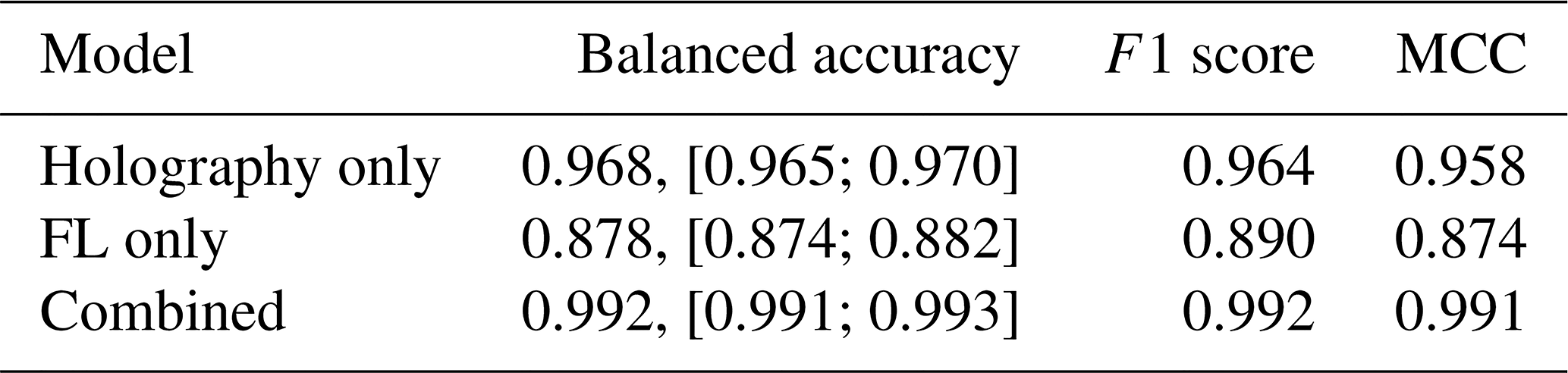
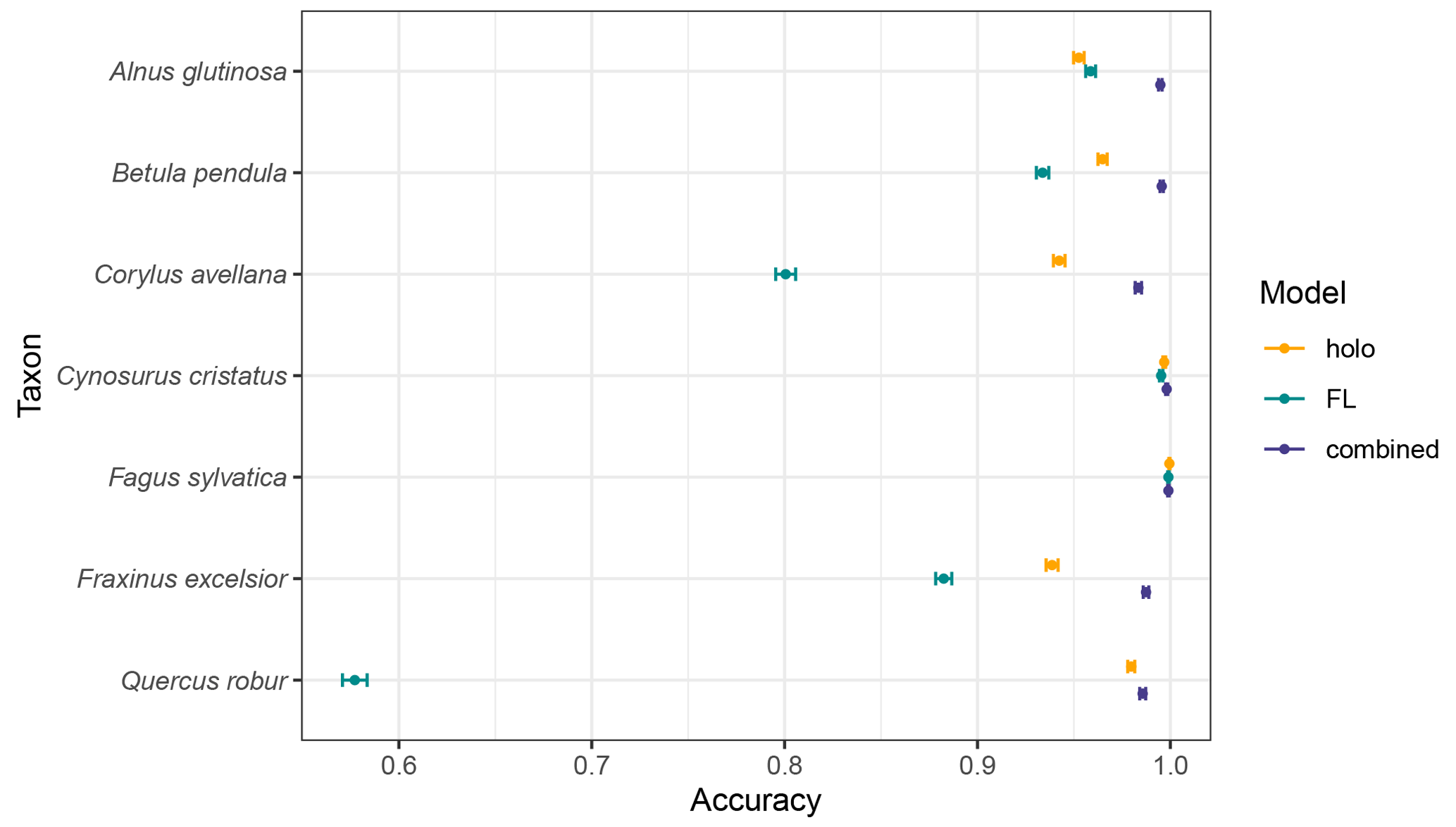
Figure 5Accuracy of each model for each taxon. The error bars represent the 95 % confidence intervals.
The results, based on measurements of aerosolised pollen grains, show that combining FL with holography leads to a substantial identification performance gain. The differences between the combined model accuracy and both single-input models confirm the findings from the UMAPs. This demonstrates that by combining the two inputs, the complementary morphological and biochemical properties of pollen grains can be used for a better classification. Although it seems small, the gain in accuracy is important for the field of aerobiology and specifically pollen monitoring since pollen grains only represent a minor part of all the particles in the air. Since pollen concentrations typically range from a few grains (<10) to a few hundred grains per cubic metre, and the thresholds for allergy symptoms are usually around tens of grains per cubic metre (Gehrig et al., 2017; Pollen.lu, 2003), misclassifications can have an impact on the information provided to allergic people. Above all, high identification accuracy is particularly important for plants with highly allergenic pollen such as Ambrosia artemisiifolia (common ragweed) as a few grains are sufficient to cause allergy symptoms.
Not only is the combined model's accuracy superior to the other models', but this gain is specifically important for some key pollen taxa. Indeed, the group of Alnus, Betula, and Corylus, all from the Betulaceae family, is known to be difficult to classify accurately and presents a very high allergic potency with possible cross-reactivity in central and northern Europe (Puc and Kasprzyk, 2013). Thus, the excellent classification performance obtained here opens the door to better monitoring by using holography together with fluorescence data. In addition, the consistent FL signal in between instruments and the available excitation sources and measurement channels characterise single pollen grains precisely even though the 405 nm excitation source was set aside. Also, the combinations of excitation and emission wavelengths used in the SwisensPoleno correspond to the most prominent fluorescence modes for a variety of dry pollen studied in Pöhlker et al. (2013). The coherence between our results and those from Pöhlker et al. (2013) brings confidence into our measurements and the stability of the SwisensPoleno. In future work, the 405 nm excitation source needs to be included to verify its potential for improvement.
When working with images, choosing neural networks for classification is the obvious solution to be sure not to lose information by using the image itself as input. However, the discrimination of pollen taxa using the UMAP dimension reduction method shows that working with features derived from the holographic images is also a possibility for pollen classification. Future work testing other machine learning methods on image features and fluorescence spectra needs to be conducted as other classifiers may perform similarly while being cheaper in terms of computational resources. In addition, the main limitation of this study, focusing on a reduced number of pollen taxa and manually aerosolised pollen, should be overcome in following work by gathering more data to train a broader model and test it on operational data.
In the end, we expect the benefit of combining holography with FL measurements for pollen classification to have a positive impact on the capacity of models to discriminate different pollen taxa. Moreover, in an operational set-up, the benefit of using FL in addition to holography could be even higher as it would allow for an easy distinction between biological and non-biological particles (e.g. water droplets, sand particles, or dust) assuming that they do not fluoresce. Yet, the extent of the gain in the real case scenario remains to be quantified as the dataset used in this study probably does not catch all the environmental variability. For example, in ambient air, pollen can break into fragments, also impacting allergy sufferers but not currently monitored.
The present study demonstrates the potential of using FL measurements as a complementary input to holographic images for single-grain pollen identification using the SwisensPoleno and ML algorithms for the most important allergy-causing pollen taxa in central Europe. The capacity of the ML model to identify pollen grains depends on both inputs, and they compensate each other when one does not provide enough information for accurate identification. As a result, the performance of the combined model is systematically higher than that of either of the models trained with a single input. The restricted and artificially aerosolised pollen dataset used in this study has several limitations but still provides strong evidence for the complementary role of FL and holography.
In conclusion, we recommend the use of relative FL as a secondary input for automatic pollen identification using the SwisensPoleno Jupiter. In this study, we tested its contribution on a restricted dataset, showing that the contribution of FL is of great value for operational networks where similar pollen taxa can be encountered. Finally, the use of relative FL for automatic pollen identification further opens the door to a larger and more precise monitoring of bioaerosols. For example, objects which are challenging to identify using holographic imaging only, such as fungal spores, could be added to the panel of particles.
The algorithms presented in this paper are experimental and subject to further development. They are available for research purposes on request to the authors of the paper. Work is in progress to further improve and stabilise them in order to make them public.
The data presented in this paper are involved in further algorithm development. They are available for research purposes on request to the authors of the paper.
SE, EG, and YZ conducted the study and contributed equally as main authors. SL guided the machine learning aspects and supervised PW in his work on the relative fluorescence. AB, BCl, GL, and FT contributed to writing, and BCr supervised the study and contributed to writing.
Elias Graf and Yanick Zeder are employees of Swisens AG. At least one of the (co-)authors is a member of the editorial board of Atmospheric Measurement Techniques. The peer-review process was guided by an independent editor. The investigations were carried out in compliance with good scientific practices, and the declared relationships have no effect on the results presented.
Publisher’s note: Copernicus Publications remains neutral with regard to jurisdictional claims made in the text, published maps, institutional affiliations, or any other geographical representation in this paper. While Copernicus Publications makes every effort to include appropriate place names, the final responsibility lies with the authors.
We would like to thank all the co-authors for their support, advice, and help in the various aspects of this study. We are grateful for such collaborations. We would also like to thank the Swiss National Science Foundation for their financial support.
This research has been supported by the Schweizerischer Nationalfonds zur Förderung der Wissenschaftlichen Forschung (grant no. IZCOZ0_198117).
This paper was edited by Rebecca Washenfelder and reviewed by two anonymous referees.
Adamov, S., Lemonis, N., Clot, B., Crouzy, B., Gehrig, R., Graber, M. J., Sallin, C., and Tummon, F.: On the measurement uncertainty of Hirst-type volumetric pollen and spore samplers, Aerobiologia, 1–15, https://doi.org/10.1007/s10453-021-09724-5, 2021.
Beggs, P. J.: Impacts of climate change on allergens and allergic diseases, Cambridge University Press, https://doi.org/10.1017/CBO9781107272859, 2016.
Buters, J., Clot, B., Galán, C., Gehrig, R., Gilge, S., Hentges, F., O'Connor, D., Sikoparija, B., Skjoth, C., Tummon, F., Adams-Groom, B., Antunes, C. M., Bruffaerts, N., Çelenk, S., Crouzy, B., Guillaud, G., Hajkova, L., Kofol Seliger, A., Oliver, G., Ribeiro, E., Rodinkova, V., Saarto, A., Sauliene, I., Sozinova, O., and Stjepanovic B.: Automatic detection of airborne pollen: an overview, Aerobiologia, 1–25, https://doi.org/10.1007/s10453-022-09750-x, 2022.
Chappuis, C., Tummon, F., Clot, B., Konzelmann, T., Calpini, B., and Crouzy, B.: Automatic pollen monitoring: first insights from hourly data, Aerobiologia, 36, 159–170, https://doi.org/10.1007/s10453-019-09619-6, 2020.
Chollet, F.: Keras, GitHub [code], https://github.com/fchollet/keras (last access: 22 April 2023), 2015.
Chicco, D. and Jurman, G.: The advantages of the Matthews correlation coefficient (MCC) over F1 score and accuracy in binary classification evaluation, BMC Genomics, 21, 6, https://doi.org/10.1186/s12864-019-6413-7, 2020.
Clot, B.: Trends in airborne pollen: an overview of 21 years of data in Neuchâtel (Switzerland), Aerobiologia, 19, 227–234, https://doi.org/10.1023/B:AERO.0000006572.53105.17, 2003.
Crouzy, B., Stella, M., Konzelmann, T., Calpini, B., and Clot, B.: All-optical automatic pollen identification: towards an operational system, Atmos. Environ., 140, 202–212, https://doi.org/10.1016/j.atmosenv.2016.05.062, 2016.
Crouzy, B., Lieberherr, G., Tummon, F., and Clot, B.: False positives: handling them operationally for automatic pollen monitoring, Aerobiologia, 38, 429–432, https://doi.org/10.1007/s10453-022-09757-4, 2022.
D'Amato, G., Pawankar, R., Vitale, C., Lanza, M., Molino, A., Stanziola, A., Sanduzzi, A., Vatrella, A., and D'Amato, M.: Climate change and air pollution: effects on respiratory allergy, Allergy Asthma Immun., 8, 391–95, https://doi.org/10.4168/aair.2016.8.5.391, 2016.
Damialis, A., Traidl-Hoffmann, C., and Treudler, R.: Climate change and pollen allergies, in: Biodiversity and Health in the Face of Climate Change, 47–66, https://doi.org/10.1007/978-3-030-02318-8_3, 2019.
Gehrig, R., Maurer, F., and Schwierz, C.: Regionale Pollenkalender der Schweiz – MeteoSchweiz, Fachbericht Nr. 264, https://www.meteosuisse.admin.ch/services-et-publications/publications/rapports-et-bulletins/2017/regionale-pollenkalender-der-schweiz.html (last access: 22 April 2023), 2017.
Greiner, A. N., Hellings, P. W., Rotiroti, G., and Scadding, G. K.: Allergic Rhinitis, The Lancet, 378, 2112–2122, https://doi.org/10.1016/S0140-6736(11)60130-X, 2011.
Halbritter, H., Bouchal, J., and Heigl, H.: Fagus sylvatica, PalDat – A palynological database, https://www.paldat.org/pub/Fagus_sylvatica/304830;jsessionid=05C006636E5F5ED57525EEC2BFCC162F (last access: 22 April 2023), 2021.
Hirst, J. M.: An automatic volumetric spore trap, Ann. Appl. Biol., 39, 257–265, https://doi.org/10.1111/j.1744-7348.1952.tb00904.x, 1952.
Huffman, J. A., Perring, A. E., Savage, N. J., Clot, B., Crouzy, B., Tummon F., Shoshanim, O., Damit, B., Schneider, J., Sivaprakasam, V., Zawadowicz, M. A., Crawford, I., Gallagher, M., Topping, D., Doughty, D. C., Hill, S. C., and Pan, Y.: Real-time sensing of bioaerosols: review and current perspectives, Aerosol Sci. Tech., 54, 465–495, https://doi.org/10.1080/02786826.2019.1664724, 2020.
Lieberherr, G., Auderset, K., Calpini, B., Clot, B., Crouzy, B., Gysel-Beer, M., Konzelmann, T., Manzano, J., Mihajlovic, A., Moallemi, A., O'Connor, D., Sikoparija, B., Sauvageat, E., Tummon, F., and Vasilatou, K.: Assessment of real-time bioaerosol particle counters using reference chamber experiments, Atmos. Meas. Tech., 14, 7693–7706, https://doi.org/10.5194/amt-14-7693-2021, 2021.
Maya-Manzano, J. M., Tummon, F., Abt, R., Allan, N., Bunderson, L., Clot, B., Crouzy, B., Daunys, G., Erb, S., Gonzalez-Alonzo, M., Graf, E., Grewling, L., Haus, J., Kadantsev, E., Kawashima, S., Martinez-Bracero, M., Matavulj, P., Mills, S., Niederberger, E., Lieberherr, G., Lucas, R. W., O'Connor, D., Oteros, J., Palamarchuk, J., Pope, F. D., Rojo, J., Sauliene, I., Schäfer, S., Schmidt-Weber, C. B., Schnitzler, M., Sikoparija, B., Skjoth, C. A., Sofiev, M., Stemmler, T., Trivino, M., Zeder, Y., and Buters, J.: Towards European automatic bioaerosol monitoring: comparison of 9 automatic pollen observational instruments with classic Hirst-type traps, Sci. Total Environ., 866, 161–220, https://doi.org/10.1016/j.scitotenv.2022.161220, 2023.
McInnes, L., Healy, J., and Melville, J.: UMAP: Uniform Manifold Approximation and Projection for dimension reduction, arXiv [preprint], https://doi.org/10.48550/arXiv.1802.03426, 2018.
Oteros, J., Pusch, G., Weichenmeier, I., Heimann, U., Möller, R., Röseler, S., Traidl-Hoffmann, C., Schmidt-Weber, C., and Buters, J. T. M.: Automatic and online pollen monitoring, Int. Arch. Allergy Imm., 167, 158–166, https://doi.org/10.1159/000436968, 2015.
Oteros, J., Buters, J., Laven, G., Röseler, S., Wachter, R., Schmidt-Weber, C., and Hofmann, F.: Errors in determining the flow rate of Hirst-Type Pollen Traps, Aerobiologia, 33, 201–210, https://doi.org/10.1007/s10453-016-9467-x, 2017.
Pawankar, R., Canonica, G., Holgate, S., Lockey, R. F., and Blaiss, M.: World Allergy Organisation (WAO) white book on allergy, World Allergy Organisation, https://doi.org/10.3388/jspaci.25.341, 2011.
Pöhlker, C., Huffman, J. A., Förster, J.-D., and Pöschl, U.: Autofluorescence of atmospheric bioaerosols: spectral fingerprints and taxonomic trends of pollen, Atmos. Meas. Tech., 6, 3369–3392, https://doi.org/10.5194/amt-6-3369-2013, 2013.
Pollen.lu: Seuils critiques – Pollens, Ministère de la Santé, CHL, http://www.pollen.lu/?qsPage=allergysteps&qsLanguage=Fra (last access: 22 April 2023), 2003.
Puc, M. and Kasprzyk, I.: The patterns of Corylus and Alnus pollen seasons and pollination periods in two Polish cities located in different climatic regions, Aerobiologia, 29, 495–511, https://doi.org/10.1007/s10453-013-9299-x, 2013.
Rantio-Lehtimäki, A.: Short, medium, and long range transported airborne particles in viability and antigenicity analyses, Aerobiologia, 10, 175–181, https://doi.org/10.1007/BF02459233, 1994.
Raschka, S.: Model evaluation, model selection, and algorithm selection in machine learning, arXiv [preprint], https://doi.org/10.48550/arXiv.1811.12808, 2020.
Ring, J., Krämer, U., Schäfer, T., and Behrendt, H.: Why are allergies increasing?, Curr. Opin. Immunol., 13, 701–708, https://doi.org/10.1016/S0952-7915(01)00282-5, 2001.
Rojo, J., Salido, P., and Pérez-Badia, R.: Flower and pollen production in the “Cornicabra” olive (Olea europaea L.) cultivar and the influence of environmental factors, Trees, 29, 1235–1245, https://doi.org/10.1007/s00468-015-1203-6, 2015.
Sauvageat, E., Zeder, Y., Auderset, K., Calpini, B., Clot, B., Crouzy, B., Konzelmann, T., Lieberherr, G., Tummon, F., and Vasilatou, K.: Real-time pollen monitoring using digital holography, Atmos. Meas. Tech., 13, 1539–1550, https://doi.org/10.5194/amt-13-1539-2020, 2020.
Sofiev, M.: On possibilities of assimilation of near-real-time pollen data by atmospheric composition models, Aerobiologia, 35, 523–531, https://doi.org/10.1007/s10453-019-09583-1, 2019.
Spieksma, F. T. M.: Pollinosis in Europe: new observations and developments, Rev. Palaeobot. Palynolo., 64, 35–40, https://doi.org/10.1016/0034-6667(90)90114-X, 1990.
Tan, M. and Le, Q.: EfficientNet: Rethinking Model Scaling for Convolutional Neural Networks, in: International conference on machine learning, PMLR, Long Beach, CA, USA, 10–15 June 2019, 97, 6105–6114, https://proceedings.mlr.press/v97/tan19a.html (last access: 22 April 2023), 2019.
Tummon, F., Adamov, S., Clot, B., Crouzy, B., Gysel-Beer, M., Kawashima, S., Lieberherr, G., Manzano, J., Markey, E., Moallemi A., and O'Connor, D.: A first evaluation of multiple automatic pollen monitors run in parallel, Aerobiologia, 1–16, https://doi.org/10.1007/s10453-021-09729-0, 2021.
Van der Walt, S., Schönberger, J. L., Nunez-Iglesias, J., Boulogne, F., Warner, J. D., Yager, N., Gouillart, E., and Yu, T.: Scikit-image: image processing in Python, PeerJ [code], 2, e453, https://doi.org/10.7717/peerj.453, 2014.
Woolcock, A. J., Bastiampillai, S. A., Marks, G. B., and Keena, V. A.: The burden of asthma in Australia, Med. J. Australia, 175, 141–145, https://doi.org/10.5694/j.1326-5377.2001.tb143062.x, 2001.
Woolcock, A. J. and Peat, J. K.: Evidence for the increase in asthma worldwide, Ciba Foundation Symposium, 206, 122–139, https://doi.org/10.1002/9780470515334.ch8, 2007.
Ziello, C., Sparks, T. H., Estrella, N., Belmonte, J., Bergmann, K. C., Bucher, E., Brighetti, M. A., Damialis, A., Detandt, M., Galán, C., Gehrig, R., Grewling, L., Guttiérrez Bustillo, A. M., Hallsdóttir, M., Kockhans-Bieda, M. C., De Linares, C., Myszkowska, D., Pàldy, A., Sánchez, A., Smith, M., Thibaudon, M., Travaglini, A., Uruska, A., Valencia-Barrera, R. M., Vokou, D., Wachter, R., de Weger, L. A., and Menzel, A.: Changes to airborne pollen counts across Europe, PloS One, 7, e34076, https://doi.org/10.1371/journal.pone.0034076, 2012.
Zuberbier, T., Lötvall, J., Simoens, S., Subramanian, S. V., and Church, M. K.: Economic burden of inadequate management of allergic diseases in the European Union: a GA2LEN review, Allergy, 69, 1275–1279, https://doi.org/10.1111/all.12470, 2014.