Evaluation of optimized flux chamber design for measurement of ammonia emission after field application of slurry with full-scale farm machinery

Field-applied liquid animal manure (slurry) is a significant source of ammonia (NH₃) emission, which is harmful to the environment and human health. To evaluate mitigation options, reliable emission measurement methods are needed. A new system of dynamic flux chambers (DFCs) with high-temporal-resolution online measurements was developed. The system was investigated in silico with computational fluid dynamics and tested using three respective field trials, with each trial assessing the variability in the measured emission after application with trailing hose at different scales: manual (handheld) application, a 3 m experimental slurry boom, and a 30 m farm-scale commercial slurry boom. For the experiments with machine application, parallel NH₃ emission measurements were made using an inverse dispersion modeling method (backward Lagrangian stochastic, bLS, modeling). The lowest coefficient of variation among replicate DFC measurements was obtained with manual application (5 %), followed by the 3 m slurry boom (14 %), and lastly the 30 m slurry boom (20 %). Conditions in DFCs resulted in a consistently higher NH₃ flux than that measured with the inverse dispersion technique, but both methods showed a similar emission reduction by injection compared with the trailing hose: 89 % by DFC and 97 % by bLS modeling. The new measurement system facilitates NH₃ emission measurement with replication after both manual and farm-scale slurry application with relatively high precision.

1 Introduction

Liquid animal manure (slurry) can be utilized as a valuable nutrient source for crop production, but it is also a significant source of ammonia (NH₃) and greenhouse gas emissions through the whole manure management chain (Uwizeye et al., 2020). Emissions of NH₃ negatively affect the environment and human health and reduce the fertilizer value of slurry. If not properly managed, there is a high potential for emission of NH₃ from the field application of slurry.

Emission depends on several factors, including the application technique, weather, and slurry and soil properties (Hafner et al., 2018; Huijsmans et al., 2016; Webb et al., 2010). However, there are significant knowledge gaps regarding the effects of factors that influence emission, including interactions. There has been an increased research effort to measure, quantify, and model emission (Beltran et al., 2021; Hafner et al., 2019; Hassouna et al., 2022; Webb et al., 2021). Recent research has investigated emission factors to improve the accuracy and precision of the national emission reporting as well as mitigation possibilities to reduce emission. Reliable quantitative measurements of management and other effects on emission are needed.

Different methods used to measure NH₃ emission after field application of slurry can be roughly sorted into two categories: micrometeorological and enclosure methods (Shah et al., 2006). Inverse dispersion methods are micrometeorological methods that can yield accurate flux measurements, as they neither alter nor manipulate the emitting area (Lemes et al., 2023) and are compatible with slurry application by farm-scale machinery (Kamp et al., 2021). With micrometeorological methods, replication is usually omitted because of the scale of the plots and cross contamination between plots, making the estimation of precision and statistical comparisons difficult. In contrast, enclosure methods, such as dynamic flux chambers (DFCs), require only a small plot area, making replication simpler (Sommer and Misselbrook, 2016). In most DFC studies, slurry has been applied manually (handheld), which is not always representative of application with farm-scale machinery, especially when there is interaction between the slurry applicator and the soil (Hafner et al., 2024; Kamp et al., 2024). Therefore, to evaluate different application methods with repetition, a system of chambers that can be used with the farm-scale machine application of slurry is needed.

An earlier generation of wind tunnels with high-temporal-resolution NH₃ measurements (described in detail in Pedersen et al., 2020) was found to have a coefficient of variation of 13 % among triplicates with manual slurry application. These earlier-generation wind tunnels can only be used with manual application. This is due to the fact that the tunnels are mounted on a metal frame that needs to be inserted into the soil; installation of the metal frame after machine application would cause the slurry to spread out in the areas in which the frame and slurry come in contact, thereby possibly altering the area exposed to slurry, the slurry infiltration, and hence the emissions.

To evaluate a new system design before construction, in silico computational fluid dynamics (CFD) simulations can be used for assessment of turbulence intensity over the soil surface. The CFD simulates the flow patterns in the DFCs under different design scenarios in order to avoid relying solely on time-consuming trial-and-error procedures. In addition, it is hard to quantify turbulence in a chamber system without modeling (Loubet et al., 1999b). CFD has gained widespread popularity for designing and optimizing the geometry of various devices and components (Scotto di Perta et al., 2016; Silva et al., 2022).

The goal of the present study was to develop a new DFC system that can be used after slurry application by farm-scale machinery as well as manual application. The new system should provide high-temporal-resolution flux estimates, have a lower inherent variation than the earlier generation, and be able to measure emissions after application by machine.

After construction, the system was tested and evaluated using three respective field trials in order to (i) compare to the earlier generation of wind tunnels described by Pedersen et al. (2020), (ii) compare flux and relative differences between two application methods measured with DFCs and inverse dispersion modeling using the backward Lagrangian stochastic (bLS) model, and (iii) quantify differences in precision after slurry application with three different methods (manual application, 3 m experimental slurry boom, and 30 m commercial slurry boom).

2 Materials and methods

The new DFCs were designed with inspiration from the laboratory chambers used by Dominique et al. (2013) and Ntinas et al. (2013). An initial design was thoroughly investigated in silico using CFD to assess the homogeneity of airflow above the emission surface and to evaluate the level of turbulence intensity within the chamber. A prototype was built after positive CFD assessment, and the recovery of NH₃ was measured with several different sample-air inlet designs. The final assessment was conducted using three respective field trials on the performance of the chambers for the measurement of NH₃ emission after application of slurry manually, by farm-scale machinery with a 30 m slurry boom, and by machinery with a smaller 3 m experimental slurry boom. For the application with machinery, measurements with inverse dispersion modeling were performed in parallel for comparison.

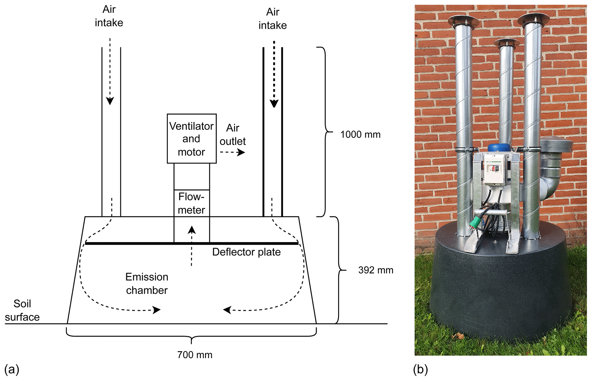
Figure 1 (a) Sketch of the dynamic flux chamber (not to scale). (b) Picture of dynamic flux chamber. The reader is also referred to Fig. S1 in the Supplement for more information.

2.1 Dynamic flux chamber

2.1.1 Chamber design

A conceptual design of cylindrical chambers with a deflector plate was chosen (Fig. 1 and Fig. S1 in the Supplement). With application by farm-scale machinery, the chamber inlet air can have elevated concentrations of NH₃ when taken close to the soil surface. Therefore, inlets are positioned 1.4 m a.s.s. (above the soil surface) to ensure an NH₃ concentration difference between air entering the chambers (background air) and the chambers' outlet air.

The emission chambers are made of slightly conical open-bottom polyethylene (PE) cylinders, with a thickness of 5–6 mm, a diameter at the bottom of 700 mm, and a height of 392 mm, giving a field plot area of 0.38 m². A deflector plate (6 mm plywood) is inserted 92 mm from the top, with 30 mm between the edge of the plate and the sides of the chambers. The design with a deflector plate was chosen to attempt to distribute the inflow air evenly above the emitting surface. Three galvanized-steel pipes (length: 1000 mm; diameter: 80 mm) are evenly distributed at the top of the chamber as air inlets. In the middle of the chamber, air is drawn in with a fan (VH 125 hætte, Lindab A/S, Viby, Denmark). An iris diaphragm (DIRU 125, Lindab A/S, Viby, Denmark) is located between the chamber and the fan to control and measure the volumetric air exchange rate (AER, in cubic meters of flow per minute per cubic meter of chamber volume), which is maintained at a fixed value during each trial.

For NH₃ analysis, sample air from the chamber is drawn at 1.5 L min⁻¹ through 15 m polyvinylidene difluoride (PVDF) tubing (o.d.: 6.35 mm; i.d.: 4.76 mm; Adtech Polymer Engineering Ltd, Stroud, UK). PVDF has been shown to have only minor NH₃ adsorption (Vaittinen et al., 2014). The tubing is insulated and heated to a minimum of 50 °C. The tubing length was 15 m so that the chambers can be used for experiments with farm-scale application machinery, which typically spreads slurry with 24–30 m slurry-booms in Denmark. For background concentrations, three tubes are attached to an air inlet at three different chambers to measure the concentration of NH₃ in the air entering the chambers.

The sampling point for outlet air was designed to optimize mixing of the air before entering the sample tube (Sect. 2.1.3 and Fig. S3 in the Supplement). Between the PVDF tube and air sampling point, a PTFE filter (diameter: 47 mm; pore size: 0.2 µm; Bohlender GmbH, Grünsfeld, Germany) is inserted to ensure that no dust or other particles enter the tubing, valve, or analyzer.

To avoid air entering the chamber from the soil surface outside the area covered by the chamber, a plastic ring (o.d.: 750 mm; height: 30 mm) is placed outside the chamber after the chamber has been placed in the field, and the space between the chamber and the ring is filled with sand (Fig. S4 in the Supplement).

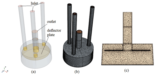
Figure 2 Schematic configuration and illustration of the mesh distribution of case A: (a) the geometry model, (b) the surface mesh, and (c) the mesh distribution at a plane of Z = 0.0 m.

2.1.2 Computational fluid dynamics

CFD modeling, conducted using the STAR-CCM+ commercial software (STAR CCM+, 2020), was used to evaluate the uniformity of airflow and the level of turbulence intensity with four different chamber configurations (height of deflector plate × AER). The aim was to design the chamber in such a way that it ensured a high degree of air mixing within the chamber and homogeneous airflow over the soil surface without dead volume (headspace without flow) or headspace with more intense turbulence compared with the rest of the headspace volume. It was not a goal to mimic ambient wind velocities or mass transfer, as these vary greatly. The chambers were designed to have a constant AER during an experiment in order to keep the measuring system simple and, therefore, more robust for field measurements. The geometric domain employed for the CFD modeling is illustrated in Fig. 2a, and the mesh distribution in the vertical central plane (Z = 0.0 m) is displayed in Fig. 2c, where the X–Z plane is located in the central plan of the chamber and the origin of Y starts from the floor of the chamber. To generate the mesh within the computational domain, a combination of polyhedral and prism meshers was used. The prism layers were generated near solid surfaces to resolve the boundary layer properly. The first layer of the mesh was placed in the position where the y+ value was either larger than 30 or smaller than 5 to fulfill the requirement of the two-layer y+ treatment wall function. The final number of the mesh utilized in the simulations was 342 354 for simulations A and B and 987 519 for simulations C and D.

The RANS (Reynolds-averaged Navier–Stokes) method was used. The realizable two-layer k-ϵ model was adopted to simulate the turbulent kinetic energy and dissipation rate of turbulent kinetic energy. The two-layer y+ wall treatment was selected. The second accuracy upwind scheme was applied to discretize the convection terms in partial differential equations (PDEs). The convergence criteria were set as 10⁻³ for continuity, with three velocity components and two turbulent quantities. Additionally, the air velocities at several points were also monitored to assist with assessment of the convergence of the simulations.

Table 1 Boundary conditions for CFD simulation scenarios.

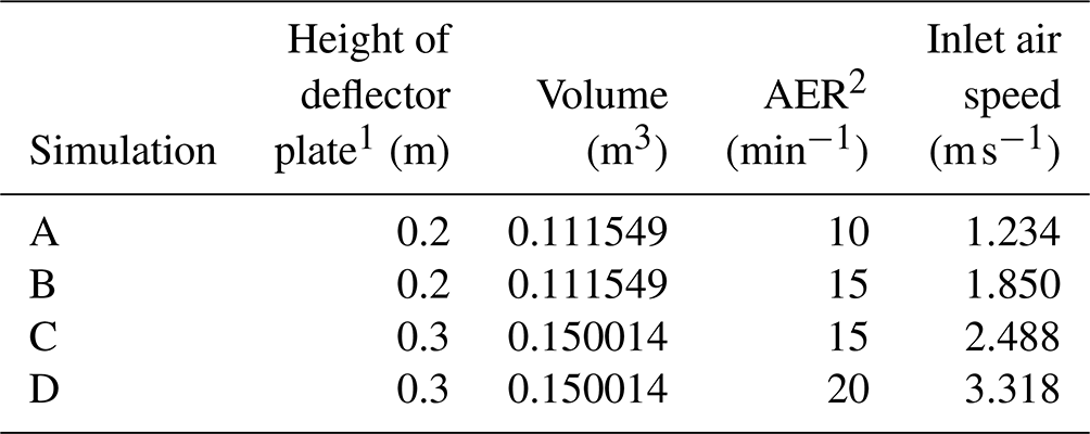
¹ Distance from the soil to the plate. ² AER stands for air exchange rate.

The CFD simulations were conducted in an isothermal condition. A no-slip condition was imposed at all solid surfaces. The inlet was set as a velocity inlet with turbulent intensity of 10 % and turbulent length scale of 0.0056 m. The outlet was defined as a pressure outlet with a pressure of 0.0 Pa. The boundary conditions for CFD simulation scenarios can be found in Table 1.

2.1.3 Recovery of ammonia, mixing within the chamber, and stability of airflow

All concentration measurements for the evaluation of the chambers were done with a cavity ring-down spectrometer (CRDS) (G2103 NH₃ concentration analyzer, Picarro, CA, USA). To evaluate the stability of measurement and recovery, NH₃ emission was measured from a solution of NH₄Cl (4 g N L⁻¹) using several different designs for sampling at the air inlet. Furthermore, the time needed for a stable concentration reading on the CRDS and the stability of the reading at two different AERs (15 and 20 min⁻¹) was evaluated after manual application of cattle slurry in bands mimicking trailing hose application.

For recovery and stability evaluation, 50 mL of the NH₄Cl solution was added to an open container (length: 150; width: 110 mm; height: 20 mm). To induce emission, the pH was increased to > 10 by adding 1 mL of 32 % NaOH. The container was then immediately placed under the tunnel, airflow through the chamber was started, and the NH₃ concentration was measured with the CRDS. Each trial lasted between 15 and 60 min. At the end of each trial, 0.5 mL of 96 % H₂SO₄ was added to the NH₄Cl solution to decrease the pH (< 4), which stopped emission. Samples of the NH₄Cl solution were taken before and after emission measurement to determine the loss of N by difference, which was then compared to the loss calculated from the concentration measurements with the CRDS and airflow. Three inlet designs were tested: a single-point design, a Y-shaped design with 15 quadratically spaced sampling points (Fig. S2 in the Supplement, corresponding to the C3u configuration from Table 1 in Loubet et al., 1999a), and a new design with the goal of optimized mixing. The new inlet design consisted of a 100 mm PTFE tube (o.d.: 6.35 mm; i.d.: 4.75 mm) inserted into a 15 mL plastic centrifuge tube which was itself inserted into a 50 mL plastic centrifuge tube. All three tubes (PTFE tube and both centrifuge tubes) had three rows of five small holes (Fig. S3).

Table 2 Overview of field trials.

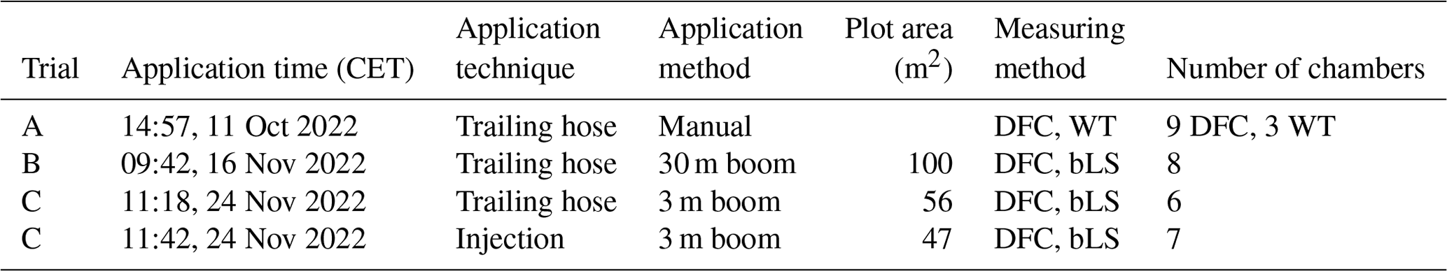
Note: the abbreviations used in the table are as follows: DFC – dynamic flux chamber; WT – wind tunnel; and bLS – backward Lagrangian stochastic model.

In a preliminary trial, six DFCs were used with manual cattle slurry application to test the stability of concentration measurements (to determine if 8 min was sufficient to reach a stable reading and if the AER affected emission dynamics). The volumetric AERs in the emission chamber were adjusted to 15 and 20 min⁻¹ to match the CFD simulations (Sect. 2.1.2), with three DFCs for each AER. Cattle slurry (1.5 L) was applied manually to a grass field in two bands to mimic trailing hose application, corresponding to an application rate of 30 t ha⁻¹. The measurements were conducted for 60 h, and the average temperature was 9.1 °C. The reader is referred to the Supplement for results.

2.2 Field trials

Three field trials were conducted in October and November 2022 at Viborg Campus, Aarhus University (Table 2). Anaerobically digested slurry (digestate) was applied using three respective application systems (manual application, 3 m experimental slurry boom, 30 m farm-scale commercial slurry boom) to assess the variability between replicates with different slurry application strategies. The trials were conducted in three different periods in the same field. Emission was measured for 60 h for trial A and for 120 h for trials B and C using the DFC. Emission data and calculations for the field trials can be found at http://github.com/AU-BCE-EE/Pedersen-2023-DFC (last access: 24 July 2024).

2.2.1 Overview of field trials

In trial A (Table 2), digestate was applied manually in bands at the soil surface with a hose connected to a watering can with a predetermined volume of digestate. In parallel, the emissions were measured with an earlier wind tunnel (WT) design setup that is described in Pedersen et al. (2020). A total of nine DFCs and three WTs were included in a block design, with each block containing three DFCs and one WT (Figs. S5 and S6 in the Supplement). The 12 chambers (DFCs and WTs) were all connected to the same valve and the same instrument for NH₃ concentration measurements, thereby eliminating the risk of biases between instruments.

For application in trial B (Table 2), a commercial 30 m trailing hose (hose diameter: 50 mm) boom (SB series, Samson Agro A/S, Viborg, Denmark) was used for digestate application. The driving speed during application was approximately 7–8 km h⁻¹. The digestate was applied in a rectangular 30 m × 70 m plot. Immediately after application, eight DFCs were placed in the plot (Figs. S7–S9 in the Supplement), and measuring points for bLS measurements were placed inside and upwind of the plot. In total, three CRDS instruments were used in trial B.

In trial C (Table 2), digestate was applied in two plots using 3 m booms especially constructed for field trials. In one plot, digestate was applied by trailing hose (hose diameter: 50 mm), whereas injection was utilized in the other plot. The driving speed during application was approximately 3.5–4 km h⁻¹. Immediately after application, six and seven DFCs were placed in the plots for trailing hose and injection application, respectively (Figs. S10–S13 in the Supplement), and a measuring point for bLS measurements was placed inside each of the two plots, with one upwind position. In total, four CRDS instruments were used in trial C.

2.2.2 Digestate and soil properties and climatic conditions during the trials

The digestate was produced at the biogas plant at Aarhus University, which operates two reactors in series at 51 °C for 14 d and 47 °C for 40 d. After the second reactor, the digestate was pumped to a concrete storage tank, where the digestate for the trials was collected. The input to the first reactor in the period during which the digestate was produced for the trials was 82 % mixed cattle and pig slurry, 9 % deep litter, and 9 % grass and grass silage (by fresh mass).

Table 3 Digestate properties (± standard deviation, n=2) and application details.

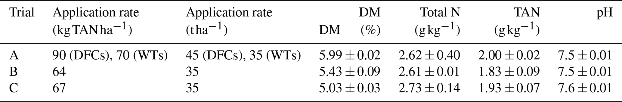
Note: the abbreviations used in the table are as follows: TAN – total ammoniacal nitrogen; DM – dry matter; N – nitrogen; DFC – dynamic flux chamber; and WT – wind tunnel.

The digestate was analyzed using standard methods for dry-matter (DM) content (American Public Health Association, 1999), total nitrogen (Association of Official Analytical Chemists, 1999), and total ammoniacal nitrogen (TAN) (International Standard, 1984). All digestate properties and application rates during the trials can be found in Table 3.

The field had a loamy sand texture with barley stubble. The gravimetric water content and dry-bulk density were determined using 100 cm³ soil cores taken at 0–5 cm depth. The dry-bulk density was 1.30 ± 0.10 g cm⁻³ (n=9). At the beginning of trials A, B, and C, the gravimetric water content was 0.19 ± 0.002, 0.22 ± 0.01, and 0.22 ± 0.01 g g⁻¹ (n=3), respectively.

Ambient air temperature was measured at a local weather station located < 0.5 km from the plot for trial A and logged as 1 h averages. For trials B and C, the average temperature and wind speed at 30 min intervals were derived from 16 Hz measurements with an ultrasonic anemometer (WindMaster, Gill, Hampshire, UK) at 2 m height. Temperature and wind speed during the trials can be found in Fig. 4.

2.2.3 Emission measurements

For all chamber emission measurements (DFCs and WTs), the NH₃ concentration was measured continuously with a model G2103 (gas concentration analyzer, Picarro, CA, USA) cavity ring-down spectrometer (CRDS), whereas two or three model G2509 analyzers (gas concentration analyzer, Picarro, CA, USA) were used for bLS NH₃ concentration measurements. These instruments have been shown to be robust and reliable in agricultural environments (Garcia et al., 2024; Kamp et al., 2019).

Dynamic flux chambers and wind tunnels

For the DFC and WT measurements, air was drawn to a 10-port rotary valve or two 10-port rotary valves connected to become one 19-port rotary valve (model C46R, C45R-8140EUTA, VICI, Valco Instruments Co. Inc., Houston, TX, USA). Measurements were done on each airstream for 8 min, yielding a data point every 144 min for trial A (nine DFCs with three backgrounds and three WTs with three backgrounds), every 88 min for trial B (eight DFCs and three backgrounds), and every 80 min for trial C (seven DFCs and three backgrounds per application method). During the trials, the AER in the DFC was set to 20 min⁻¹.

Each WT consisted of an open-bottomed stainless-steel chamber (height: 250 mm; length: 800 mm; width: 400 mm). The airflow through the chamber was controlled with a fan, motor, and frequency converter that was connected to the emission chamber via a steel duct. The air inlet was a narrow 130 mm high slot. The AER was set to 25 min⁻¹. Each WT was mounted on a metal frame inserted into the soil, giving a field-plot area of 0.2 m². Sample air was drawn through a heated PTFE tube (o.d.: 6.35 mm; i.d.: 4.75 mm). A detailed description of the WT can be found in Pedersen et al. (2020).

For both DFCs and WTs, an average of the last 30 s of measurements per 8 min measurement cycle was used for calculation of the flux and cumulative emission. An average of the background measurements (n=3 with respect to locations) was subtracted for each measurement cycle concentration before further calculations were carried out. The background-corrected concentration (C, mg m⁻³), the airflow in the emission chamber (q, m³ s⁻¹), and the area of the soil surface covered by the tunnel (A, m²) were used to calculate the flux (F, $\mathrm{mg}{\mathrm{s}}^{-\mathrm{1}}{\mathrm{m}}^{-\mathrm{2}}$) as follows:

$$\begin{array}{}\text{(1)}& F={\displaystyle \frac{C\cdot q}{A}}.\end{array}$$

The contribution from each measurement cycle to the cumulative emission was calculated from the flux using the trapezoidal rule.

The backward Lagrangian stochastic method

An inverse dispersion model, the backward Lagrangian stochastic (bLS) model, was used to obtain NH₃ fluxes in trails B and C. The bLS model has previously been used to estimate NH₃ emissions after slurry application (Hafner et al., 2024; Kamp et al., 2021), and it simulates air movement backwards in time from the origin of the sensor based on the wind field in a certain averaging interval (in these trials, 30 min intervals). The bLS model was used with the bLSmodelR R software package (https://github.com/ChHaeni/bLSmodelR, last access: 24 July 2024, version 4.3; Häni et al., 2018), which produces a concentration-to-emission ratio (CE_bLS) for each averaging interval.

The flux (F) is calculated using the concentration-to-emission (CE) value in combination with the NH₃ concentrations measured upwind (C_upwind) and downwind (C_downwind) of the source:

$$\begin{array}{}\text{(2)}& F={\displaystyle \frac{(C_{\text{downwind}}-C_{\text{upwind}})}{{\mathrm{CE}}_{\mathrm{bLS}}}}.\end{array}$$

The inputs to the bLS model are the friction velocity (u*), the roughness length (z₀), the Obukhov length (L), the standard deviation of the three wind components (σ_u, σ_v, and σ_w), and the wind direction. In these two trials, 100 000 trajectories were used in the model calculations. The positions of the source and sensor are also inputs to the model, and the positions were mapped with a GPS (Trimble R10, Sunnyvale, California, USA). A detailed explanation of the bLS model can be found in Häni et al. (2018).

The atmospheric conditions affect the accuracy of the bLS model, and the method is most accurate under conditions where the Monin–Obukhov similarity theory can reasonably be applied (McBain and Desjardins, 2005). Thus, observations were filtered (removed) when $u^{\ast }\le$ 0.05 m s⁻¹, |L| ≤ 2 m, z₀ > 0.1 m, ${\mathit{\sigma }}_u/u^{\ast }$ > 4.5, and ${\mathit{\sigma }}_v/u^{\ast }$ > 4.5 (Bühler et al., 2021; Lemes et al., 2022). Flux was estimated by linear interpolation in these intervals for calculation of cumulative emission.

For trial C, three CRDS instruments were used to measure ambient NH₃ in the field before digestate application. The concentration for all three instruments was stable for 9.5 h before application, and there was a small offset between the instruments. In that time span, the instruments' average background concentrations were 1.920 ± 0.06, 0.273 ± 0.03, and 0.824 ± 0.11 µg NH₃ m⁻³ for the instruments later used for the injection plot, trailing hose plot, and background, respectively. The instruments for the injection plot and trailing hose plot were corrected for the offset by subtracting 1.096 µg NH₃ m⁻³ and adding 0.551 µg NH₃ m⁻³, respectively. The difference was very small compared with the measured background concentrations of NH₃. However, for this trial, the concentration difference between background and the plots was low; thus, the small offset would have influenced the fluxes from the injection plot if not corrected.

2.2.4 Statistics for comparing emission measurements

Emission measurements were compared in multiple ways. They were normalized by applied TAN, expressed as a percentage lost per minute, and compared graphically for each trial. Total cumulative emission was expressed as a percentage of applied TAN. For methods with replication (DFCs and WTs), a mean value, standard deviation, and coefficient of variation (CV, standard deviation divided by the mean) were calculated from the individual estimates determined with each separate chamber.

Differences in variability or precision between DFCs and WTs as well as among application methods were primarily assessed by comparing CV values. Moreover, a detailed analysis of the flux over time from DFCs and WTs with manual application was performed using a gamma generalized linear mixed model defined with the logarithmic link function and a random component representing the tunnel or the chamber and with a factor representing the elapsed time (following a statistical methodology similar to that in other emission studies such as Pedersen et al., 2021a, b). Separate models were adjusted for the WT and DFC measurements, facilitating a comparison of the variability obtained with the two measurement methods by comparing the estimated dispersion parameters. As the variances of the responses under a gamma model are proportional to the square of the expected value of the response, with a proportionality coefficient given by the dispersion parameter (which was different for the two methods), the variance of the two methods was compared by examining the two curves relating the predicted variance to the predicted means.

Trial C provided an opportunity to compare the application method effects measured with the new DFC design to bLS measurements. Replicate DFC measurements from trailing hose application and injection were used together to calculate a 95 % confidence interval on the relative emission reduction provided by injection. For this task, the unit of analysis was an individual DFC, while the response variable was total cumulative emission as a percentage of applied TAN. The t.test() function in R (stats package, v4.2.1; R Core Team 2023) was used with log₁₀-transformed values to simplify the calculation of a relative effect. Estimated 95 % confidence limits based on separate estimates of variance for each group and the Welch modification to degrees of freedom were back-transformed to express the reduction as a percentage of trailing hose emissions. A bootstrap approach based on resampling was also applied for comparison (Davison and Hinkley, 1997).

The bLS measurements were not replicated, making it difficult to estimate random error. An important source of error for the bLS method is bias between instruments, especially when the concentration differences are small, as for the injection plot in particular. Therefore, an estimate of uncertainty related to potential instrument bias in concentration measurements was made. Although this estimate does not include all potential sources of error, because the two plots were in the same field and measurements occurred at the same time, other sources of error are likely to be similar for the two plots and, therefore, less important for the estimation of a relative difference. A standard deviation in the overall concentration bias was based on background measurements made by the three instruments over a 9.5 h period prior to digestate application (Sect. 2.2.3) combined with measurements from a 30 h period 10 d after application, when any effect of slurry application was expected to be negligible. Because there is no replication for concentration measurements, this standard deviation provides a direct estimate of how bias may vary for a randomly selected instrument. As emission calculations depend on the concentration difference (Eq. 2), a value for the difference between two instruments (s_bd, for the standard deviation of the two-instrument bias in measurement of a concentration difference) was estimated using the formula for independent errors (Eq. 3.13 in Taylor, 1982). Uncertainty in an individual emission measurement interval can then be calculated by using this value as the numerator in Eq. (2). Assuming constant bias over a trial, the overall standard deviation in measured emission was estimated using Eq. (3), where CE_bLS is an average concentration-to-emission ratio over the emission measurement trial duration, Δt is the interval duration (0.5 h = 1800 s), and n_int is the number of intervals (240).

$$\begin{array}{}\text{(3)}& s_{\text{emis}}={\displaystyle \frac{s_{\text{bd}}}{{\mathrm{CE}}_{\mathrm{bLS}}}}\mathrm{\Delta }t\cdot n_{\text{int}}\end{array}$$

This estimate of the standard deviation in the measured emission was applied to both plots using a parametric bootstrap approach to estimate the 95 % confidence interval for the relative reduction (Davison and Hinkley, 1997).

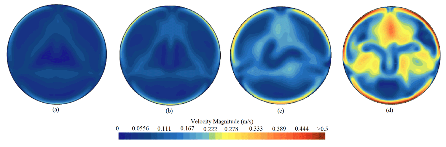
Figure 3 Velocity distribution at a horizontal plane 0.05 $\mathrm{m}\mathrm{a}.\mathrm{s}.\mathrm{s}.$ for (a) a deflector plate height of 0.2 m and air exchange rate (AER) of 10 min⁻¹, (b) a deflector plate height of 0.2 m and AER of 15 min⁻¹, (c) a deflector plate height of 0.3 m and AER of 15 min⁻¹, and (d) a deflector height of 0.3 m and AER of 20 min⁻¹.

3 Results and discussion

3.1 Velocity magnitude of computational fluid dynamics

Figure 3 displays the velocity magnitude distribution at a horizontal plane 0.05 $\mathrm{m}\mathrm{a}.\mathrm{s}.\mathrm{s}.$ When the AER was 10 min⁻¹ the velocity magnitude was smaller than 0.17 m s⁻¹ (Fig. 3a). When the AER was 15 min⁻¹ and the deflector plate was 0.2 $\mathrm{m}\mathrm{a}.\mathrm{s}.\mathrm{s}.$, the velocity magnitude was up to about 0.15 m s⁻¹ if the relatively higher air speed near the edge of the chamber was not considered (Fig. 3b). With the deflector height of 0.3 $\mathrm{m}\mathrm{a}.\mathrm{s}.\mathrm{s}.$, the average velocity magnitude of the plane was about 0.2 m s⁻¹ (Fig. 3c). Although the deflector plate is placed 0.10 m higher in Fig. 3c compared with that in Fig. 3b with the same AER of 15 min⁻¹, the inlet air speed is 2.49 m s⁻¹ in case of Fig. 3c, whereas it was 1.85 m s⁻¹ in case of Fig. 3b. Thus, the velocity magnitude is still slightly higher in Fig. 3c. As the AER was increased to 20 min⁻¹ in the case shown in Fig. 3d with a deflector plate height of 0.3 m, the velocity magnitude of the plane was notably increased, up to 0.45 m s⁻¹. The increase in the velocity magnitude with a higher AER was also found by Saha et al. (2011), who studied the airflow in wind tunnels with different dimensions of cross-sectional area using CFD. In order to ensure that the velocity was high enough for the air within the chamber to be well mixed and avoid any “dead zones” over the soil surface, a plate height of 0.3 m and an AER of 20 min⁻¹ were chosen for the field experiments (Fig. 3).

3.2 Recovery of ammonia, mixing within chamber, and stability of airflow

Both the single-point measurement and the Y-shaped measuring inlet resulted in very unstable measurements: concentrations could change by up to several hundred parts per billion (> 35 % of average) within a few seconds (data not shown). The final inlet design (Sect. 2.1.3 and Fig. S3) was found to give steady measurements in the range of concentrations found after slurry application (15–2500 ppb). The final inlet design gave an average recovery of emitted NH₃ of 102 ± 1 % (mean ± standard deviation, n=3) from the NH₄Cl test. This high recovery shows that irreversible adsorption is insignificant in the concentration range measured during the recovery test (800–3000 ppb); however, at lower concentrations, adsorption might cause longer response times.

The two different AERs did not yield different emission dynamics (Fig. S14 in the Supplement), but emission was lower with the lower AER. Similar results have been observed earlier, with a prior study finding that an increasing AER increased emissions (Hafner et al., 2024). There was no difference in the concentration measurement stabilization time with the two different AERs (Fig. S15 in the Supplement), and an 8 min measurement period was sufficient to reach a stable reading, except for the first round of measurements, which is a known issue due to the adsorption of NH₃ on all surfaces in the measurement system (Pedersen et al., 2020).

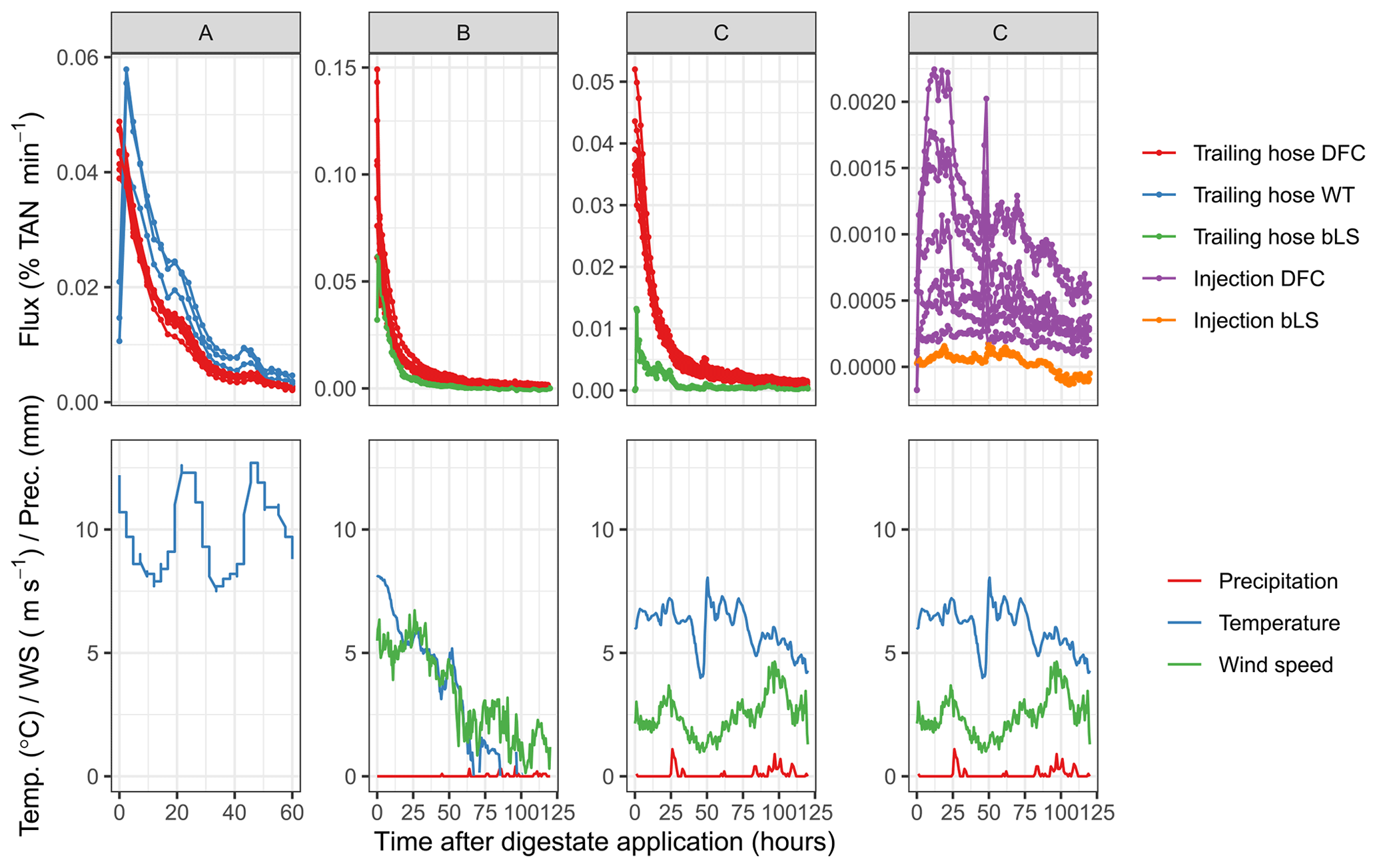
Figure 4 Ammonia emission rate (as a fraction of applied TAN per minute) and weather after the application of digestate by trailing hose or injection measured with dynamic flux chambers (DFCs), wind tunnels (WTs), or a backward Lagrangian stochastic (bLS) model. Digestate was applied manually (a), by 30 m boom (b), or by 3 m boom (c). Note that the y-axis scales differ.

3.3 Field trials

3.3.1 Performance of dynamic flow chambers

The new DFC design performed better than the earlier-generation WT design, with less of a delay or lag in initial emission measurements and lower variability in emission among replicates. The DFCs did not show the same lagging effect during the first measurement as the WTs (Fig. 4). Lagging in the first WT measurement will cause an underestimation of the cumulative NH₃ emission (Hafner et al., 2024; Pedersen et al., 2020). The improvement with the new DFC design is likely due to better heating of the sampling lines or the alternate tube material (PVDF), which has a lower affinity for NH₃ adsorption compared with PTFE (Vaittinen et al., 2014). Furthermore, the improved sampling lines likely reduce the general lagging effect which causes slight under- or overestimations of the NH₃ concentrations measured, on the order of 1 %–3.5 % for tubes heated to a lower temperature, depending on the concentration of the preceding measurement (Pedersen et al., 2020).

The gamma generalized linear mixed models adjusted well (p values for a goodness of fit equal to 0.62 and 0.89 for the DFCs and the WTs, respectively; see Figs. S16 and S17 in the Supplement for quantile–quantile plots). The dispersion parameters were estimated as 2.2 × 10⁻⁵ and 3.3 × 10⁻⁵ for the models describing the DFC and the WT determinations, respectively. This indicates that the WT fluxes were characterized by a substantially larger variability compared with the DFCs (Fig. 5).

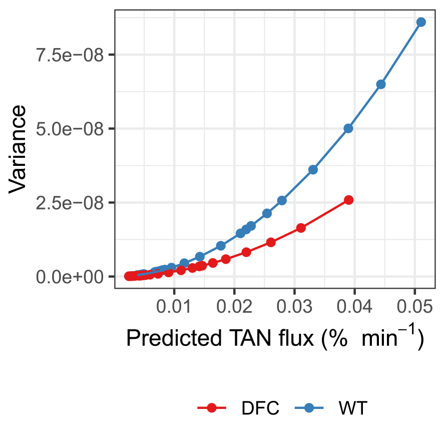
Figure 5 Theoretical variance expressed as a function of the theoretical mean of NH₃ flux measurements with dynamic flux chambers (DFCs) and wind tunnels (WTs) after trailing hose application of digestate.

Table 4 Cumulative ammonia loss (% TAN) measured with dynamic flux chambers (DFCs), wind tunnels (WTs), and a backward Lagrangian stochastic (bLS) model after the application of digestate by trailing hose or injection manually, with a 3 m boom, or with a 30 m boom. The mean, the number of observations for chamber methods (n), the standard deviation (SD), and the coefficient of variation (CV) are reported for DFCs and WTs.

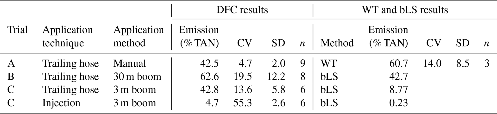
Ammonia emission measurements after field application of slurry has at least three sources of variation: error inherent in emission measurement systems, uneven slurry application, and heterogeneity in soil properties that affect emission. The last two sources are expected to contribute to variation in measurements with enclosure methods to a higher degree than measurements with micrometeorological methods because of their small plot size. As expected, the standard deviation and coefficient of variation increased in the following order: manual application < 3 m boom < 30 m boom (Table 4). This was expected because it is possible to evenly apply the slurry close to the soil surface when using manual application, resulting in a uniform application in all bands. When applying slurry with a 30 m boom, it is expected that there can be differences in the amount of slurry leaving each hose, due to variation in the length from the distributor, potential plugging, or other differences between hoses which will cause variation in the local application rate and exposed slurry surface area along the boom. Furthermore, the higher driving speed using the 30 m boom application compared with the 3 m boom application is expected to also cause higher variation in the exposed surface area of each digestate band, as the higher speed causes more movement in each individual trailing hose, especially over uneven soil surfaces. The same field was used, but the plot area between the trials differed in the present study (Figs. S5, S7, and S10). Therefore, the main cause of the variation is most likely the application itself and not soil heterogeneity, as the soil heterogeneity is likely minor within the area where the tunnels are placed between the three trials.

The differences in variation between the application methods indicate that it will be possible to detect much smaller differences between treatments if slurry is applied manually compared with machine application. Based on the standard deviation values (Table 4), for an equal sample size (number of DFCs), manual application could be used to detect a difference that is a factor of 5 to 6 smaller, compared with the 30 m boom. Although there is still some difference between manual and machine application, manual application might be applicable when mimicking trailing hose application and when slurry properties are the parameters investigated. The relatively large variation with machine application makes it difficult to compare different low-application techniques to each other. To properly compare any application methods in which there is a direct physical interaction between soil and the application machinery (e.g., trailing shoes and injection), it is necessary to apply the slurry with farm-scale machinery to get a realistic response. In some cases, the differences between different low-emission application techniques can be small (10 %–20 % of emission; Häni et al., 2016; Webb et al., 2010), in which case it would most likely not be possible to detect differences with a system such as the one presented in the present paper.

This high variation for application by machinery indicates that more measurement replicates (DFCs) are needed, compared with manual application. This difference should be carefully considered when planning field trials due to the trade-off between replicates and the number of different treatments that can be tested.

Although this new DFC design was only used for NH₃ from field-applied slurry, it should also work for other sources and other compounds. Other DFC designs have been used for NH₃ from mineral fertilizer and volatile organic compounds from slurry (Pedersen et al., 2021c; Scotto di Perta et al., 2020). Measuring less-adsorbing compounds than NH₃ could even allow for a higher temporal resolution of the measurements.

3.3.2 Comparison with inverse dispersion measurements

The NH₃ flux, and consequently cumulative emission, measured with the DFCs was much higher than that from the bLS measurements in the two trials that included both measuring methods (trials B and C; Fig. 4, Table 4). Other studies have also found an over- or underestimation of NH₃ emissions measured with flux chambers compared with micrometeorological methods (Hafner et al., 2024; Kamp et al., 2024; Mannheim et al., 1995; Misselbrook et al., 2005; Ryden and Lockyer, 1985; Scotto di Perta et al., 2019). Previous studies have reported that the difference between chamber and micrometeorological measurements can primarily be attributed to air-side mass transfer and rainfall (Eklund, 1992; Hafner et al., 2024; Smith and Watts, 1994; Sommer and Misselbrook, 2016). It is likely that this is also the case in this study, as the measurements were conducted in the same field plot after farm machine application; hence, the differences cannot be attributed to differences caused by slurry, application, or soil. During both trials with parallel bLS measurements, the ambient wind speed was relatively low (Fig. 4), and slight precipitation also occurred during trial C, which likely contributed to low emissions for the bLS measurements.

Considering uncertainty in measured emission based on random error for DFCs and concentration bias for the bLS measurements, both the reduction in emission (injection compared with trailing hose) and emission following injection were similar between the two methods. Both methods showed low emission after injection. For DFC measurements, the 95 % confidence interval was 2.3 % to 7.1 % of applied TAN (n=7 chambers), compared with −1.8 % to 2.4 % of applied TAN for bLS for injection. For trailing hose application, the intervals were 37 % to 49 % of applied TAN (n=6 chambers) for DFCs and 9.9 % to 15 % of applied TAN for bLS measurements. The NH₃ emission reduction obtained by injecting the digestate compared with application by trailing hose was measured to be 89 % with DFC measurements, with a 95 % confidence interval of 83 % to 95 % (or 85 % to 93 % from the bootstrap approach). For bLS measurements, the reduction was 97 % relative to trailing hose emission. Uncertainty for bLS measurement was 1.2 % of applied TAN (s_emis), which is a relatively small value, although large compared with a loss of 0.23 %, resulting in a confidence interval of 74 %–100 % (assuming that a reduction > 100 %, representing uptake of atmospheric NH₃ after slurry application, is not plausible). Thus, the range for reduction obtained by injection is similar for DFCs (83 %–95 %) and bLS measurements (74 %–100 %). Uncertainty in the bLS measurement results here reflect challenges with respect to measuring a small concentration increase compared to the background level, which was a consequence of a small plot and very efficient slurry injection. Using a small plot means that the source area was very small compared with the concentration footprint area (Kamp et al., 2021).

4 Conclusions

A new dynamic flux chamber measurement system with online measurements showed lower variability than an earlier-generation system of wind tunnels. For trials with trailing hose application, variability increased drastically from manual (handheld) application (coefficient of variation, CV = 5 %) to application with a 3 m slurry boom (14 % CV), and even further for application with a 30 m farm-scale slurry boom (20 % CV). This increase in variability can potentially make it difficult to measure small differences between treatments when slurry is applied by machine, unless larger sample sizes (more repetitions) are used. The differences in variation between handheld application and machine application should be taken into consideration when planning field trials. The flux measured with DFCs was consistently higher than the bLS-measured flux from the same plot in two experiments, with differences likely caused by the relatively high air exchange rate in the DFCs. Due to this difference, the new DFC design with the chosen AER should not be used for the estimation of open-air emissions, but it can be used to estimate relative differences between application methods or slurry treatments.