the Creative Commons Attribution 4.0 License.
the Creative Commons Attribution 4.0 License.
 | 08 Aug 2024
Reliable water vapour isotopic composition measurements at low humidity using frequency-stabilised cavity ring-down spectroscopy
Amaelle Landais
Tim Stoltmann
Justin Chaillot
Mathieu Daëron
Fréderic Prié
Baptiste Bordet
Samir Kassi
In situ measurements of water vapour isotopic composition in polar regions has provided needed constrains of post-deposition processes involved in the archiving of the climatic signal in ice core records. During polar winter, the temperatures, and thus the specific humidity, are so low that current commercial techniques are not able to measure the vapour isotopic composition with enough precision. Here, we make use of new developments in infrared spectroscopy and combine an optical-feedback frequency-stabilised laser source (OFFS technique) using a V-shaped cavity optical feedback (VCOF) cavity and a high-finesse cavity ring-down spectroscopy (CRDS) cavity to increase the signal-to-noise ratio while measuring absorption transitions of water isotopes. We present a laboratory infrared spectrometer leveraging all these techniques dedicated to measure water vapour isotopic composition at low humidity levels. At 400 ppmv, the instrument demonstrates a precision of 0.01 ‰ and 0.1 ‰ in δ18O and d-excess, respectively, for an integration time of 2 min. This set-up yields an isotopic composition precision below 1 ‰ at water mixing ratios down to 4 ppmv, which suggests an extrapolated precision in δ18O of 1.5 ‰ at 1 ppmv. Indeed, thanks to the stabilisation of the laser by the VCOF, the instrument exhibits extremely low drift and very high signal-to-noise ratio. The instrument is not hindered by a strong isotope–humidity response which at low humidity can create extensive biases on commercial instruments.
- Article
(3838 KB) - Full-text XML
- BibTeX
- EndNote


Water isotopic composition is commonly used as an atmospheric tracer (Galewsky et al., 2016) or in paleoclimate studies (Casado, 2018; Jouzel and Masson-Delmotte, 2010). Indeed, water stable isotope concentrations are modified throughout the hydrological cycle (Dansgaard, 1964); in particular at each phase transition (Craig and Gordon, 1965; Majoube, 1971; Merlivat and Nief, 1967), heavier isotopes are preferentially found in the condensed phase rather than the vapour phase (Jouzel and Masson-Delmotte, 2010). This property is paramount to the isotopic paleothermometer (Dansgaard, 1964; Lorius et al., 1969), which links the variations in isotopic composition in an ice core record to past temperatures (EPICA, 2004; North Greenland Ice Core Project members, 2004). While the isotopic paleothermometer is generally admitted to be a reliable paleoclimate proxy (Jouzel and Masson-Delmotte, 2010), in low-accumulation regions, complex post-deposition processes (Casado et al., 2018; Ekaykin et al., 2002) can modify the recorded signal (Casado et al., 2021; Steen-Larsen et al., 2014) and limit the interpretation as a past temperature record (Casado et al., 2020; Laepple et al., 2018).
Studying water vapour isotopic composition in polar regions (Casado et al., 2016; Steen-Larsen et al., 2013) is key to a comprehensive understanding of the processes affecting water isotopes in cold, dry environments, usually characterised by low accumulation (Berkelhammer et al., 2016; Bonne et al., 2019; Bréant et al., 2019; Casado et al., 2018; Ritter et al., 2016). However, in the low-accumulation regions of the poles, vapour monitoring of isotopic composition is sparse (Wei et al., 2019) and for the coldest sites limited to summer. Indeed, these measurements are mostly based on Picarro commercial instruments (Steig et al., 2014), for which the precision drops dramatically for humidity levels below 100 ppmv (Leroy-Dos Santos et al., 2021). Throughout this paper, we will use Picarro instruments as a benchmark for commercial instruments considering how ubiquitous they are in water vapour isotopic composition monitoring. In general, the amount of sublimation and condensation is poorly known during the winter months (Genthon et al., 2016), and there is no instrument able to monitor the atmospheric vapour isotopic composition due to the extremely low humidities (below 100 ppmv) (Casado et al., 2016; Ritter et al., 2016). This is despite attempts for a new generation of infrared spectrometers which are able in laboratory environments to reach humidity as low as 20 ppmv (Landsberg et al., 2014). At the site of Dome C, where the longest ice core has been drilled, humidity levels below 100 ppmv are found for 79 % of the year and below 20 ppmv for 56 % of the year (Genthon et al., 2022), yielding an urgent need for vapour isotopic composition monitoring able to measure in conditions as dry as 1 ppmv.
Applications of infrared spectroscopy techniques to water isotopic monitoring are dominated by two techniques: optical-feedback cavity-enhanced absorption spectroscopy (OF-CEAS) (Landsberg et al., 2014) and cavity ring-down spectroscopy (CRDS) (Romanini et al., 1997; Steig et al., 2014). The advantage of the former is using optical feedback (Laurent et al., 1989) to stabilise and refine the laser source and measure the absorption features associated with molecular transitions in a high-finesse resonating cavity (Morville et al., 2005). The latter on the other hand takes advantage of the extreme sensitivity of the CRDS technique (Čermák et al., 2018) to perform very precise absorption spectroscopy.
Here, building on recent efforts to combine the advantages of both techniques (Burkart and Kassi, 2015; Chaillot et al., 2023; Stoltmann et al., 2017), we present a new generation of infrared spectrometers able to measure water isotopic composition at extremely low humidities (less than 1 ppmv or equivalent to a water pressure of 0.06 Pa). These conditions are indeed commonly found in central Antarctica during the long polar winters when temperature can reach −90 °C but are also potentially found in the stratosphere or on other planets. This instrument, called VCOF-CRDS (V-shaped cavity optical feedback – cavity ring-down spectroscopy), is able to reach a precision of 0.01 ‰ and 0.1 ‰ for monitoring vapour δ18O and d-excess (second-order parameter d-exc = δD−8δ18O), respectively, and should reach satisfactory performance at humidities around 1 ppmv. Overall, the instrument achieves a precision roughly 20 times better than available commercial instruments, as well as a stability 20 times longer. An ingenious auto-referencing of the instruments also limits the impact of long-term drift of the laser and reduces the need for drift correction through regular calibration. While the current prototype cannot be deployed in the field due to its relative bulkiness (1 m3), weight, and fragility, this paper intends to provide a proof of concept for the application of this technology for the monitoring of water vapour isotopic composition at humidity levels down to 1 ppmv.
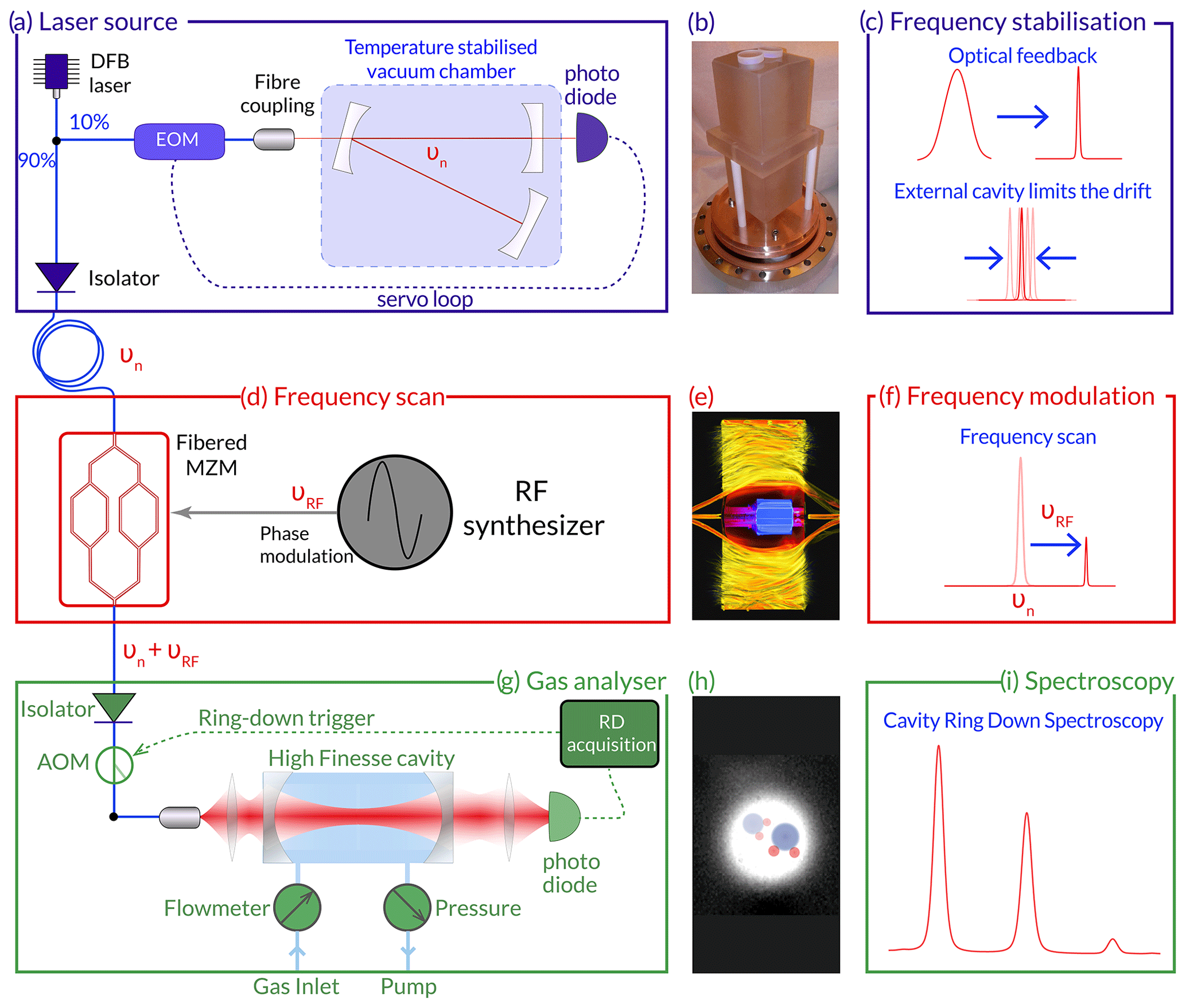
Figure 1Experimental set-up schematics: (a) the laser source, (b) a picture of the monoblock Zerodur V-shape stabilisation cavity, (c) the impact of the optical cavity on the linewidth and the drift of the laser source, (d) frequency scanner through a Mach–Zehnder modulator (MZM), (e) AI-generated representation of a MZM, (f) illustration of the sideband generation through the MZM, (g) the CRDS cavity used to analyse the gas, (h) silhouette of two water molecules drawn on top of an IR picture of the mode of the cavity, and (i) a schematic spectrum for the considered transition line (see Fig. 2).
2.1 Description of the instrument
The instrument is based on optical-feedback frequency stabilisation (OFFS) cavity ring-down spectroscopy (CRDS), a technique developed for CO2 isotope monitoring (Burkart et al., 2014; Stoltmann et al., 2017) and transferred here to water isotopic composition measurement. It includes three modules: a laser source, a frequency scanner, and a gas analyser (see Fig. 1).
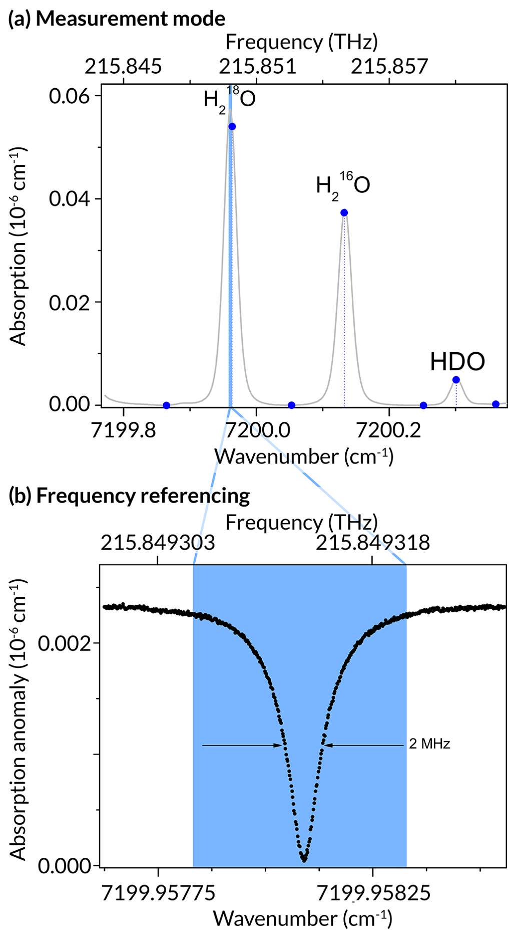
Figure 2Absorption spectra realised by the instrument: (a) in high-pace measurement mode at 400 ppmv and 35 mbar (blue dots), compared to a slow full spectrum (grey points), and illustration of the area scanned for frequency referencing (blue shaded area); (b) in frequency-referencing mode at 0.1 mbar – a feature of a Lamb-dip saturated absorption pattern used to evaluate the drift of the instrument when deployed in the field where comb assisted spectroscopy is not possible.
The light source is primarily composed of a fibred distributed feedback (DFB) laser diode (Eblana Photonics) stabilised by optical feedback (Fig. 1a) in a monoblock Zerodur V-shaped cavity (Fig. 1b). The optical power of the laser diode is approximately 20 mW by operating it at a temperature of 20.997 °C with a 122 mA current. The mirrors (LAYERTEC) have a reflectivity of 0.99992, leading to a cavity with a finesse of 131 000. The frequency stabilisation leads to the narrowing of the linewidth of the crude DFB diode from a few megahertz (MHz) to less than 70 Hz (Fig. 1c), with a drift below 2 Hz s−1 (Casado et al., 2022). The long-term drift in particular drops below 1 Hz s−1 and is dominated by the ageing of the Zerodur glass (Jobert et al., 2022) providing from a spectroscopy point of view long-term stability of the instrument, and thus, reducing the need for calibration to compensate the drift. The entire laser source set-up is regulated at 26 °C by heating elements and PT1000 temperature sensors as described in Casado et al. (2022) and Jobert et al. (2022).
The frequency scanner relies on a fibred Mach–Zehnder modulator (MZM; Fig. 1d and e) (Izutsu et al., 1981), which enables tuning of the frequency of the light source while preserving its spectral purity (Burkart et al., 2013). We apply an electrical radio-frequency signal to shift the sidebands generated by the MZM (Fig. 1f) and set up the polarisation so only a single sideband is preserved, while the other and the carrier are destroyed by negative interferences. The remaining power is around 0.9 mW, and we use a fibred optical amplifier to increase the power to 11 mW.
The light is then injected into a second cavity which is used for monitoring the isotopic composition of the water vapour based on CRDS (Fig. 1g). The CRDS cavity consists of a 48 cm long copper cylinder, with a diameter of 7 cm in which a hole of 0.8 cm has been drilled over the full length. The reflectivity of the mirrors (LAYERTEC) is 0.99995, leading to a finesse of 170 000. The length of the CRDS cavity can be adjusted by a piezoceramic actuator which moves one of the mirrors. This is used to adjust the length of the CRDS cavity, and thus its resonance frequency, to match the frequency of the light injected. As mentioned above, the power injected to the cavity is amplified to 11 mW to increase the signal-to-noise ratio on the photodiode while ensuring that saturation is not affecting the absorption profile of the gas inside the cavity (Kassi et al., 2018). An optical power of roughly 1 mW exits the CRDS cavity and is collimated on a Hamamatsu photodiode. The gas is injected in the cavity using pressure and flow controllers (Bronkhorst). The cavity is maintained at a pressure of 35 mbar (± 0.01 mbar) and the flow at 25 sccm to limit turbulence within the airflow. The entire gas analyser (Fig. 1g) is stabilised using a Peltier device (Supercool) at a temperature of 28 °C. The CRDS cavity is stabilised using a heating wire and PT1000 temperature sensors at 29.000 °C.
2.2 Spectroscopic analysis
The instrument is set such that the laser source produces light in an extremely stable manner at exactly 7199.7 cm−1, the frequency of which is then shifted using solely the MZM. The instrument can then be used in two ways: slow full spectrum mode and high-pace measurement mode.
In full spectrum mode, the instrument has a high spectral resolution and can be used to realise spectroscopy studies (Kassi et al., 2018), with a sensitivity of 10−12 cm−1 after 60 s. At high-pace measurement mode, i.e. using the instrument as a tool to monitor water vapour isotopic composition, the pace of the measurement is key in order to avoid the gas concentration changing during the course of a spectrum. Instead of measuring spectra including a large number of data points, in this case, we opt for a large number of spectra with few data points at the most relevant frequencies to characterise the absorption lines. This is done by “jumping” exactly one free spectral range (FSR) of the CRDS cavity using the MZM. With this approach, the spectral data points are spaced by multiples of the FSR (around 297 MHz), but relocking is instantaneous. By preventing any changes in gas composition throughout the duration of the scan (0.3 s), this technique improves on higher-resolution scans (up to 1 min), which, while potentially more precise, are often far slower. Fast variations in humidity level during a scan create large uncertainty in the fitting procedure which leads to additional fluctuations in the isotopic composition that are not averaged due to their auto-correlated features. The high-pace scans are associated with higher instantaneous noise with little auto-correlation which can be averaged out rapidly. As a result, when the high-pace scans are averaged out to the acquisition time of the slow-pace measurements, the precision of the average high-pace scans is better than the precision of single slow-pace scans.
In the high-pace measurement mode, the spectra are composed of seven data points (one at the top of each transition, and four for the baseline; Fig. 2a) and are realised in approximately 0.3 s when averaging together 10 ring downs per spectral point. We fitted a slow-pace, high-precision spectrum using a speed-dependent Nelkin–Ghatak profile (SDNGP) (Long et al., 2011), similarly to the approach used to measure CO2 isotopic composition (Stoltmann et al., 2017) to fix pressure- and temperature-dependent parameters. As temperature and pressure are constant, these parameters can be fixed, which reduced the number of free parameters. We then were able to generate a simple, multi-linear conversion matrix which could link the intensity of each transition in the spectra to the concentration of each isotope.
2.3 Frequency referencing
Even though the drift of the laser source is extremely limited (below 2 Hz s−1), at the scale of several hours, this can lead to significant deviations in the frequency, which leads to drift of the measured isotopic composition. This issue is general for infrared spectrometers and is usually tackled by post-correction of empirically established drift of the measurement of the isotopic composition itself (Leroy-Dos Santos et al., 2021). For previous VCOF set-ups, the frequency of the VCOF has been locked on an optical frequency comb which is itself locked on the GPS signal (Gotti et al., 2018). Here, we propose instead to measure a Lamb-dip saturated absorption feature to counteract the drift of the laser source. Indeed, at low pressure, the number of molecules can be so low that a dip feature appears at the centre of saturated absorption transitions (Fig. 2b) (Burkart et al., 2015; Kassi et al., 2018). These features are characterised by very small linewidth (below 20 kHz if the pressure is low enough), and their frequency, which remains constant for constant conditions of pressure, can be used as a frequency reference.
Here, we make use of this property to evaluate the frequency drift of the laser source by scanning every hour the Lamb-dip feature associated with the O transition at 7199.96 cm−1. To do so, we decrease the pressure inside the cavity down to 0.1 mbar, let the cavity stabilise to these new experimental conditions for 2 min, and then measure the Lamb-dip feature across 4 MHz at extremely high resolution (30 kHz) for 7 min. This method provides us with frequency measurements of the Lamb-dip-feature centre with a precision of 2.5 kHz in a single scan (Kassi et al., 2018). During a period of 140 h, we measure the frequency deviation from the Lamb-dip method, which reproduces exactly the ones estimated from the measurement of a beat note with an optical frequency comb locked on a GPS (Burkart et al., 2014) (Fig. 3), with a correlation between the two times series of r2 = 0.995 (p < 0.05). The pressure is then increased back to 35 mbar within 30 s. This leads to a biased isotopic composition measurement for another 3 min, after which we can measure again the vapour isotopic composition. The overall duty cycle here was around 80 %, including 13 min every hour during which the instrument was not able to monitor isotopic composition. Improvements on the VCOF laser source as recommended in Jobert et al. (2022) could limit the need for such self-referencing cycles. Here, we used this measurement of the deviation of the frequency of the laser source as a self-referencing method which can be applied every hour to ensure that the deviation of the laser source frequency remains smaller than 10 kHz.
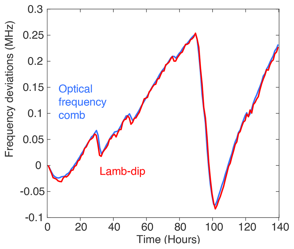
Figure 3Frequency deviation of the laser source as measured from the beat note of the laser with an optical frequency comb (blue), compared to measurements from the centre of a lamb-dip saturated absorption feature (red).
2.4 Generation of water vapour standards
We used the water vapour generator instrument described in Leroy-Dos Santos et al. (2021) to generate stable humidity levels to evaluate the response of the infrared spectrometer to varying humidity levels. We used dry-air synthetic bottles with less than 3 ppmv of water to supply the gas to the instrument. We used laboratory standards of water with isotopic compositions varying from 0 ‰ to −60 ‰ to supply water of known isotopic composition. The water vapour generator shows relatively good performance down to humidities around 20 ppmv where outgassing from the instrument itself limits its performance. As a result, we used the water vapour generator to evaluate the precision as a function of humidity (Sect. 3.1) and the humidity response of the instrument (Sect. 3.2) down to 25 ppmv.
To obtain an evaluation of the precision of the instrument below these humidity levels, we connected a dry-air bottle directly to the instrument and regulated the produced humidity levels from outgassing of the tube by changing the flux of dry air to an exhaust connected to a sonic nozzle. Using this method, humidity levels down to 4 ppmv could be reached. In this case, the isotopic composition is not known, so it cannot be used to evaluate the accuracy of the instrument; it can only be used to evaluate how stable the instrument is in measuring the relative stable isotopic composition of the outgassing water from the tube walls. As the temperature of the tube and the dry-air canister were not regulated or monitored, the resulting water vapour was relatively variable (variations around 10 % of the produced humidity level), which leads to potential variability in the isotopic composition, leading itself to relatively high Allan standard deviations not necessarily linked to the poor performance of the instrument.
We discuss the performance of the instrument first with the precision and the long-term drift of the instrument; second with the accuracy of the instrument, including the humidity-to-isotope and isotope-to-isotope relationships; and finally by highlighting the impacts of the frequency auto-referencing on the performance of the instrument.
3.1 Precision and drift
The VCOF-CRDS instrument precision has been evaluated by measuring water standards at various humidity levels generated by the calibration device described in Leroy-Dos Santos et al. (2021). To evaluate the drift in measured isotopic composition associated with the technique directly and not that impacted by the potential drift of the laser source, we used an optical frequency comb referenced to a GPS system to actively correct the frequency drift of the laser source. The impact of drift and the mitigation by the frequency auto-referencing scheme are detailed in Sect. 3.3. We generated repeated injections of the same water samples at the same conditions to generate water concentrations as stable as possible that are measured by the instrument continuously. Typically, at 400 ppmv, this resulted in successive stable humidity levels lasting up to 10 h, followed by a drop in the humidity to refill the syringe (Fig. A1). The instrument then needs up to 1 h to generate stable water again. This leads to time series of stable vapour content that can last several days but include gaps. We modified the traditional calculation of Allan variance to take gaps into account to calculate the precision as well as the drift of the instrument in a range of humidities from 20 to 1500 ppmv despite the gaps during the refill of the vapour generator.
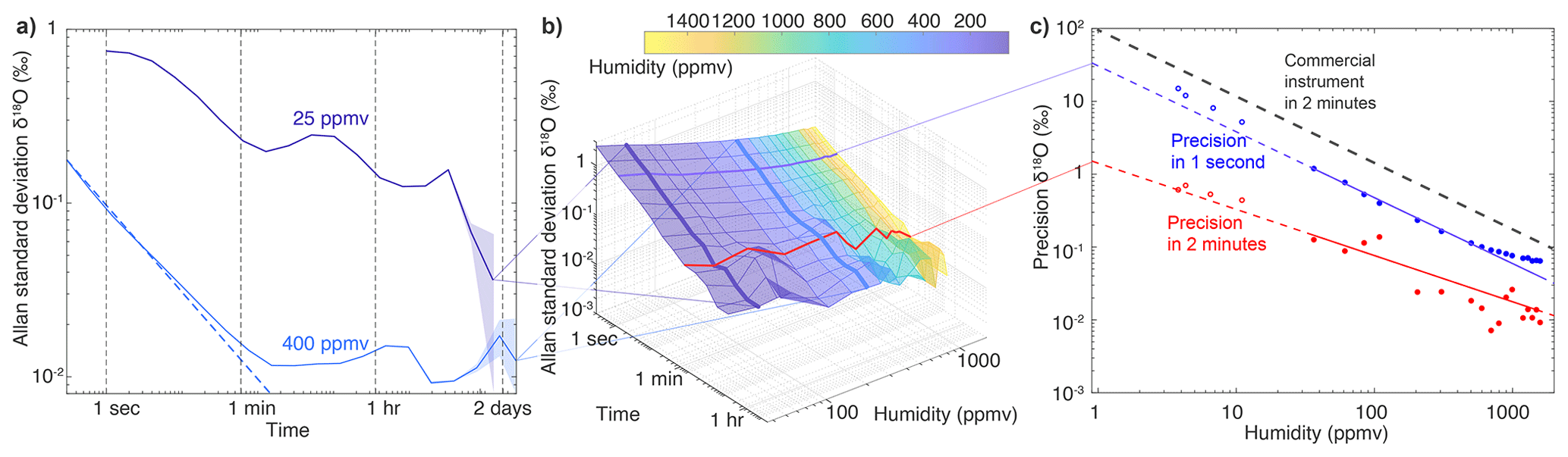
Figure 4Allan standard deviation plots of the δ18O measurements of the VCOF-CRDS instrument stabilised with an optical frequency comb: (a) long-term Allan standard deviation plots realised at humidity levels of 25 and 400 ppmv with stable measurements of 7 d; (b) 3D plot of the Allan standard deviation for different timescales and humidity levels; and (c) evaluation of the precision of the instrument across humidity levels (dots) for measurements averaged over 1 s (blue) and 2 min (red), as well as fit with a power law (solid line) and extrapolation from the fit at lower humidities that could not be reached with the calibration device (Leroy-Dos Santos et al., 2021). Additional measurements between 3 and 10 ppmv obtained from outgassing tubes (Sect. 2.4) are included on the graph as upper limits of the precision below 25 ppmv, compared to typical commercial instrument behaviour (dashed grey line, linear approximation of the performance of a Picarro L2140i extracted from Fig. 3 of Leroy-Dos Santos et al., 2021, and of a Picarro L2130i from Casado et al., 2016).
To evaluate both the short- and long-term stability of the signal, we monitored a constant humidity level of 400 ppmv for 7 d (Fig. 4a). At the temporal resolution of the instrument (3 Hz), the precision is roughly 0.2 ‰ in δ18O at a humidity of 400 ppmv and below 0.1 ‰ at 1 Hz. Under these conditions, a Picarro L2130i in HDO mode only reaches a precision of 2 ‰ at 1 Hz (Casado et al., 2016). The Allan standard deviation follows the behaviour of white noise (characterised by a decrease) until approximately 150 s when a limit value of roughly 0.01 ‰ in δ18O variations is reached. The precision remains at this lowest value for durations longer than 2 d. Similarly, for d-excess, the instantaneous precision at 400 ppmv is roughly 2 ‰ and drops to 0.1 ‰ after 150 s (Fig. 5). We chose to showcase δ18O and d-excess (instead of δD) because correlated drift between the two first-order isotopic compositions (Appendix B) leads to an Allan standard deviation of d-excess characterised with excess noise compared to both the Allan standard deviations of δ18O and δD (Fig. B1). The fundamental flicker noise limit (flat Allan deviation for times longer than 2 min) could be linked either to the instable gas generation (variable humidity and pressure) or to the measurement technique itself. At low humidity (25 ppmv), more correlated noise appears, with a decrease in the Allan standard deviation not following the law. After 1 min, a precision of 0.2 ‰ in δ18O is reached and maintained for scales longer than 1 d (we chose not to interpret the drop after 6 h below 0.1 ‰, as it is only visible in the last two points of the Allan standard deviation). Similarly, the instantaneous precision (1 s) of the instrument in d-excess at low humidity is very high (around 10 ‰) and slowly drops to 2 ‰ at around 1 min.
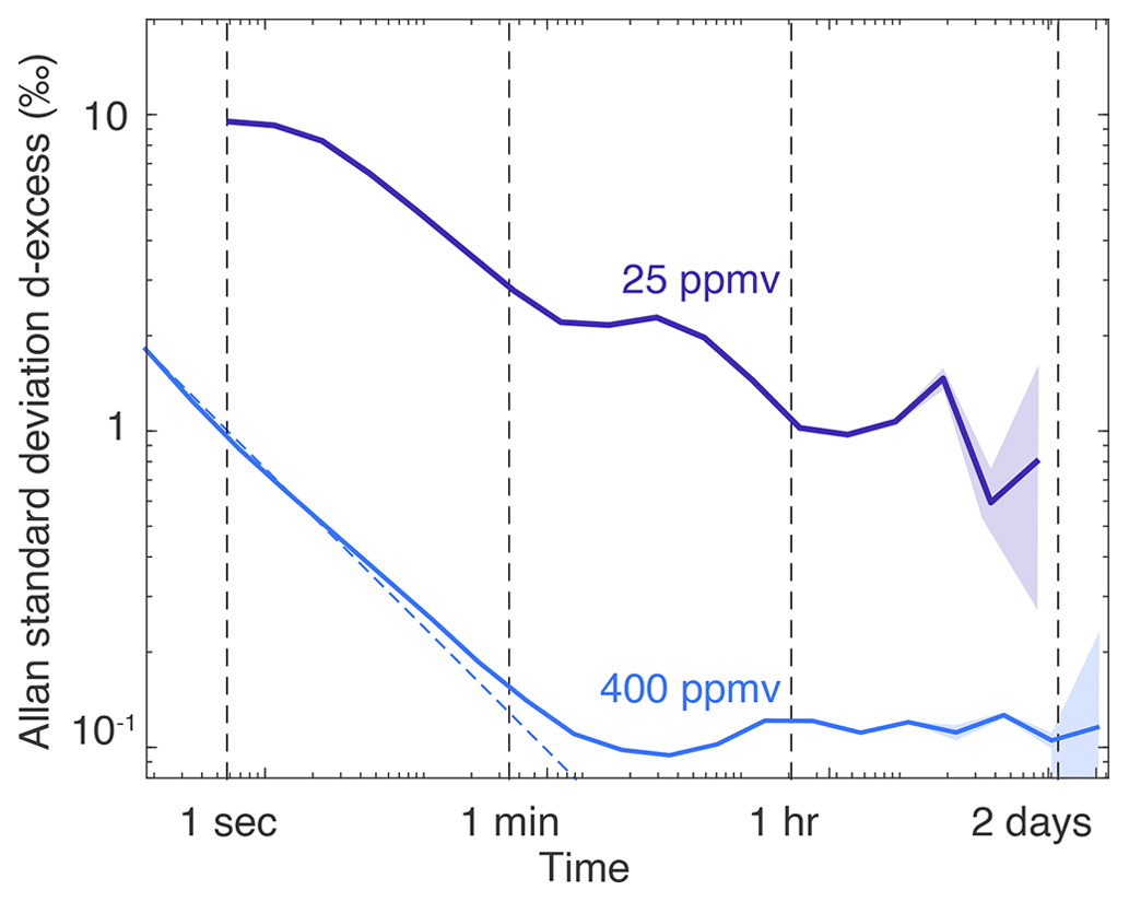
Figure 5Same as Fig. 4a for the d-excess: long-term Allan standard deviation plots realised at humidity levels of 25 and 400 ppmv with stable measurements of 7 d.
The change in precision scales with humidity as shown in Fig. 4c. So at 1 s, the precision of the instrument at 30 ppmv is roughly 2 ‰ in δ18O (roughly 10 times larger than at 400 ppmv since the humidity is approximately 10 times smaller), and the precision in δ18O at 30 ppmv drops to 0.1 ‰ after 800 s (Fig. 4b). Reciprocally, at 800 ppmv, the precision in δ18O is around 0.1 ‰ at 1 s, dropping to 0.005 ‰ after 800 s. While we were not able to generate stable moisture flux at 1 ppmv using the humidity generated as described in Leroy-Dos Santos et al. (2021), we extrapolated the precision expected after 2 min at humidity lower than 25 ppmv by fitting the data with a power law and found a precision of 1.5 ‰ at roughly 1 ppmv. We also directly connected the instrument to dry-air bottle controlling the humidity from the outgassing of the tubes connecting the bottle to the instrument (see Methods, Sect. 2.4) and evaluated the precision at 3.8, 4.2, 6.5, and 11 ppmv. Since this method to generate water standard is extremely dependent on temperature variations, it is only useful as an upper bound of the precision of the instrument as the humidity levels are relatively variable (standard deviation of the humidity larger than 10 % of the humidity content), and thus, these data points were not included in the power law fit. We find precisions ranging from 0.5 ‰ to 0.7 ‰ after 2 min (Fig. 4c), which agree relatively well with the power law defined at higher humidity levels.
3.2 Accuracy of the instrument
Infrared spectrometers tend to be biased and require calibration for the dependency of their measurements with respect to change in humidity and isotopic composition itself. To evaluate the humidity response of the VCOF-CRDS, we used the water vapour generator to generate different humidity levels and evaluate how the measured isotopic composition deviates at low humidity from the expected value for the given standard. Here, we illustrate the behaviour of the infrared spectrometer for varying humidity levels. We show a nearly flat humidity response for humidity levels above 200 ppmv (Fig. 6).
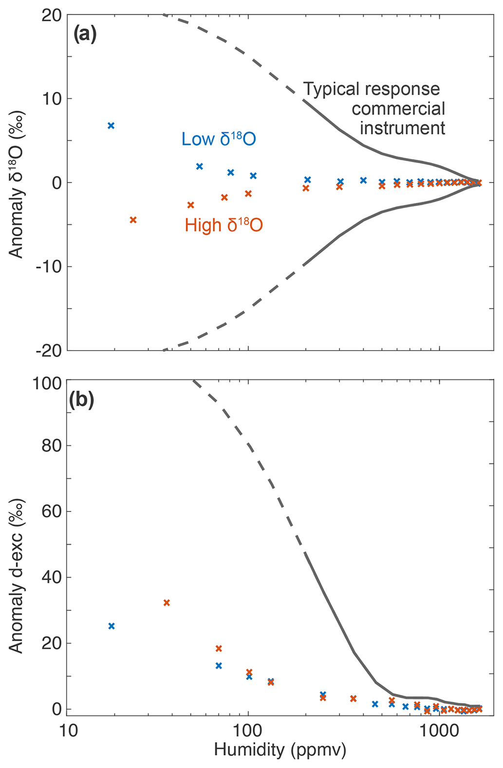
Figure 6Isotope–humidity dependence for two isotopic compositions: evaluation of the anomaly of the measurement against the value of the standard of (a) δ18O and (b) d-excess for local distilled tap water (high δ18O, approximately −7.5 ‰, orange) and depleted Antarctic water (low δ18O, approximately −50.6 ‰, blue) compared to typical response from a commercial instrument at low humidity (grey lines, extracted from the Eqs. (4) and (5) in Leroy-Dos Santos et al., 2021, based on a Picarro L2140i: solid line – humidity range where the regression was made from the observations; dashed line – extrapolation).
Infrared spectrometers usually have an isotopic response of the measurements to changes in humidity levels that needs to be corrected with an appropriate instrument (Leroy-Dos Santos et al., 2021; Weng et al., 2020). Weng et al. (2020) suggested that the humidity response of the measurement of the isotopic composition, in particular the fact that this response is different for different isotopic composition, is linked to spectroscopic effects in Picarro instruments (grey lines in Fig. 6) rather than background humidity or memory effects, at least at the first order. Here, we show that the improved frequency stabilisation and the new fit parameters provide a much flatter isotope–humidity response for both δ18O and d-excess. The amplitude of the isotope–humidity calibration changes is indeed one of the largest limitations in interpreting vapour isotopic composition at low-humidity conditions (Casado et al., 2016; Leroy-Dos Santos et al., 2020). In particular, in Antarctica where humidity falls below 500 ppmv frequently, the correction applied to δ18O and d-excess (at 100 ppmv, up to 15 ‰ and 100 ‰, respectively) can be 1 order of magnitude larger than the signal (diurnal cycle around 5 ‰ and 10 ‰, respectively, at Dome C; Casado et al., 2016). Here, the amplitude of the correction remains below 1 ‰ and 10 ‰, respectively, for humidities larger than 100 ppmv.
Additionally, for Picarro instruments, the humidity response is very variable in between individual instruments (Weng et al., 2020) and needs to be evaluated for each new analyser, as well as each time an analyser is deployed (Leroy-Dos Santos et al., 2021). The limited humidity response of our set-up is therefore extremely valuable but would need to be validated on a second VCOF-CRDS instrument to be confirmed.
Another aspect of the accuracy of isotopic analysers is the linearity of the instrument or its isotope–isotope response. We evaluated the accuracy of the new instrument on the V-SMOW–V-SLAP (Vienna Standard Mean Ocean Water and Vienna Standard Light Antarctic Precipitation) scale by measuring six internal standards from our institute, ranging from −54 ‰ to +0.5 ‰. We used the water vapour generator (Leroy-Dos Santos et al., 2021) to generate stable humidity levels of 90 min and included the average value of the last 15 min. As this water vapour generator is not as versatile as an automatic sampling device, injecting water with different isotopic composition (especially across a range of dozens of per mil) is cumbersome due to extended memory effects in the humidity generator, and it was necessary to wait more than 12 h to do a new isotopic sample. The measured δ18O aligns perfectly with the internal standard values (r2 virtually undifferentiable from 1, N=9), and the residuals of the linear regression have a standard deviation of 0.04 ‰ (Fig. 7).
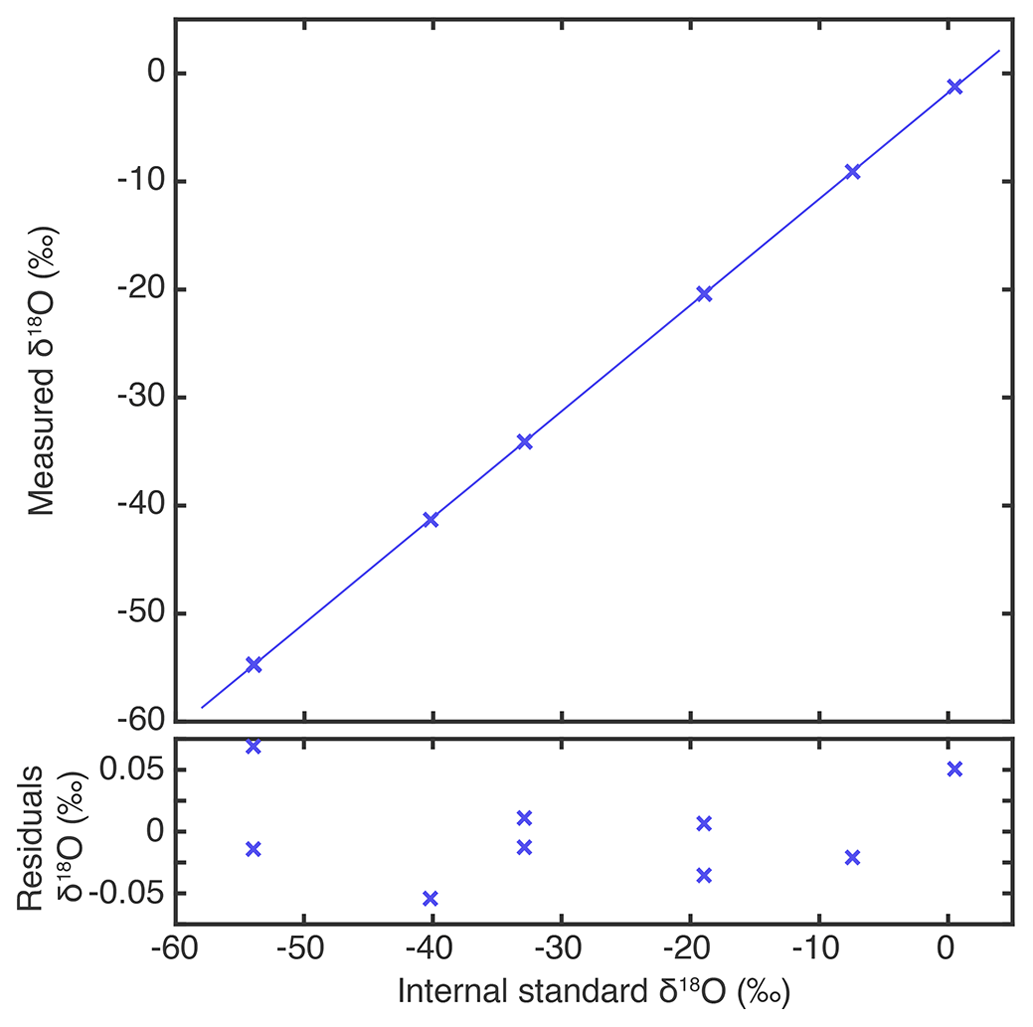
Figure 7Isotope–isotope response: measurements of internal standards referenced at average humidity of 800 to 1200 ppmv on the SMOW–SLAP scale and linear regression of the measured values against the standard values, compared to the residues.
This demonstrates the linearity of the isotopic measurement of the VCOF-CRDS. Overall, isotopic monitoring via the CRDS technique has been demonstrated to be extremely linear, even outside of the range of the isotopic compositions used for calibration (Casado et al., 2016; Steig et al., 2014). In practice, for isotopic composition measurements of ice core samples, it would be necessary to use the same sample preparation line (auto-sampler and vaporiser) for samples and calibration. If the residuals had the same type of distribution (standard deviation around 0.04 ‰) to reach an accuracy of 0.01 ‰ in δ18O, it would be necessary to perform calibrations on a smaller range of isotopic compositions or to include more measurements of the standards.
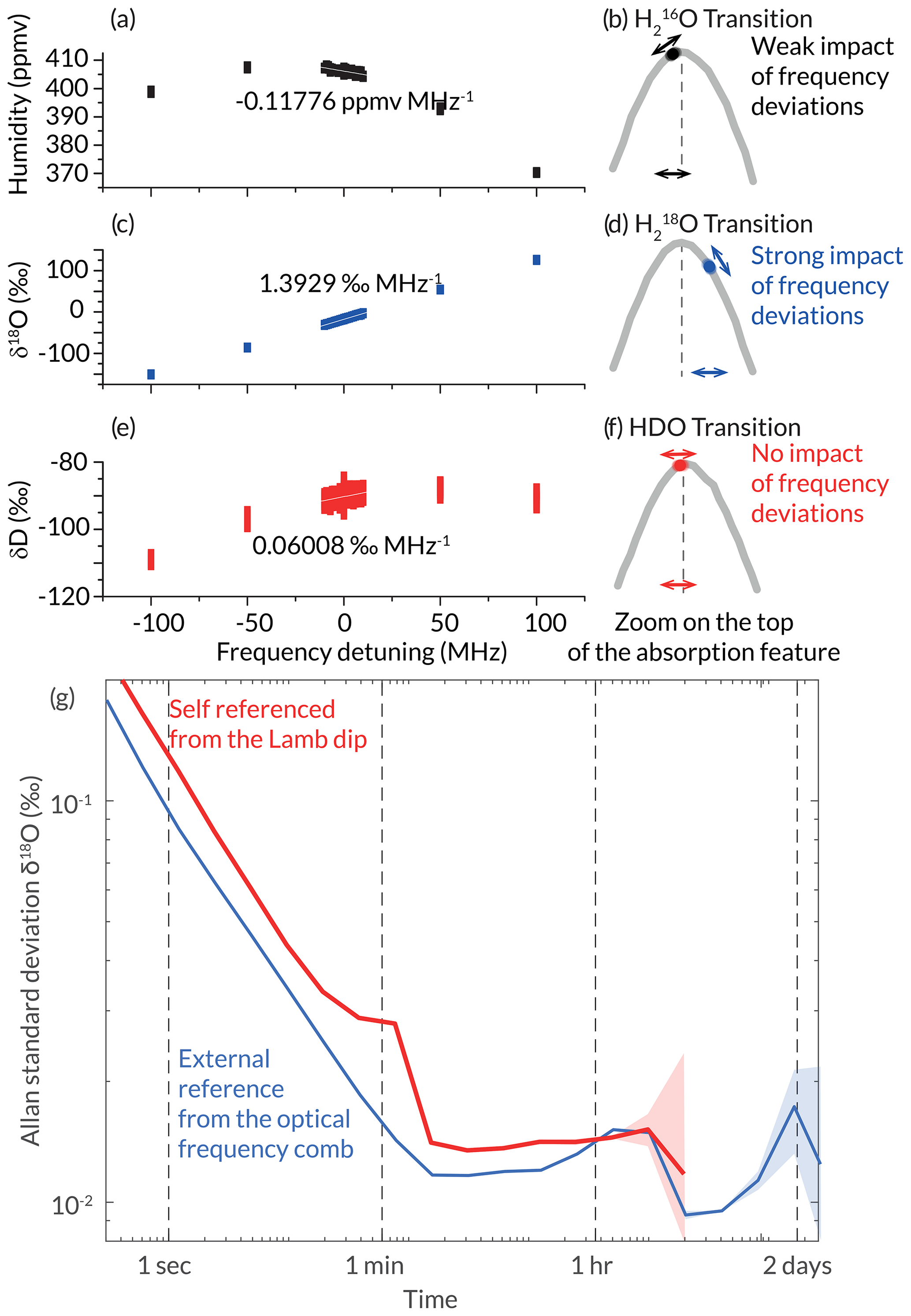
Figure 8Evaluation of the impact of the frequency drift of the laser source on the measurements of isotopic composition: impact of the frequency detuning on the measured (a) humidity, (c) δ18O, and (e) d-excess with an illustration of the positions of spectroscopic measurement points compared to their respective transition centre (b), (d), and (f). (g) Allan standard deviation of δ18O for the instrument being self-referenced (red) and with an external frequency reference (blue) at 400 ppmv.
3.3 Frequency auto-referencing
The main source of uncertainty for the measurement comes from the drift of the light emission frequency of the laser source. Indeed, since the frequency scan is only used to reach the successive resonance mode of the CRDS cavity, the spectra produced in high-pace measurement mode are not necessarily exactly aligned with the absorption lines. For the current cavity, with an FSR of 297 MHz, it was not possible to have data points exactly on top of all three scanned transitions, and in particular, the spectral point for the O transition is relatively far from the transition centre (Fig. 8d).
We evaluated the impact of frequency drift on the measurement uncertainty by artificially adding frequency detuning during the frequency scanning system measuring the same gas in stable conditions. The added detuning of the frequency ranged from −100 to +100 MHz with a 50 MHz resolution, as well as every 1 MHz between −10 and +10 MHz (Fig. 8a, c, and e). For the HDO transition where the measurement point was the closest to the transition centre, we observe no impact of the frequency detuning. For the humidity measurement, a small impact is observed (around 0.1 ppmv MHz−1) linked to the small distance of the spectroscopic measurement to the centre of the absorption feature. The main impact for our current set-up is on δ18O, for which a sensitivity to drift of roughly 1.4 ‰ MHz−1 is observed. Considering the current performance of the laser source (1.7 Hz s−1; Casado et al., 2022), this leads to a drift of the δ18O of roughly 0.008 ‰ h−1 or up to 0.2 ‰ d−1. This is much greater than the performance obtained in Fig. 4a at timescales longer than 1 h, which suggests that at long timescales, this would be the dominating source of uncertainty.
In order to maintain the performance around 0.01 ‰ for δ18O for averages longer than 2 min, we need to include frequency referencing every hour. We implemented the frequency auto-referencing mode described in Sect. 2.3 and measured Lamb-dip features every hour. The frequency drift of the laser source measured by this technique was then compensated for directly in the frequency modulation by the MZM. Note that no extrapolation of future drift is implemented, so the frequency added on the frequency modulation is a step which is updated every hour when a new Lamb dip is measured. The use of the Lamb-dip self-referencing approach enables us to actively correct all frequency deviations of the VCOF laser source (Fig. 1a), leading to the performance displayed in Fig. 8g.
We compare the Allan standard deviation of the measurement of a constant sample made with this self-referenced mode of the instrument with the Allan standard deviation with the external frequency reference (Fig. 8g). For timescales shorter than 1 h, an excess noise is added to the data probably due to the step approach to correct the drift. An extrapolation from a given number of the previous Lamb-dip measurements could potentially on average fix part of this excess noise but with the risk of over-correction when the environmental conditions shift. Since a satisfactory precision can be reached after 5 min despite this excess noise, this has not been implemented. For timescales longer than 1 h, the performance of the instrument with the self-referencing matches exactly the ones with external frequency referencing. The measurement of δD is not affected as the measurement point is perfectly centred on the transition.
Changing the length of the CRDS cavity so the FSR aligns the frequency of the measurement at the top of all the transitions would mitigate a large part of the drift impact on δ18O (this is equivalent to finding an FSR equal to the common denominator between the difference in frequency between the three transitions). This solution will be favoured for instruments deployed in the field and would limit the need to implement frequency auto-referencing to every 6 h.
Major new study topics arising from the capacity of infrared spectrometers to measure the isotopic composition at low humidities include water vapour monitoring in very cold field conditions, as well as the evaluation of the fractionation coefficients of heavy isotopes with respect to light isotopes (Majoube, 1971).
Current commercial instruments are limited to measure isotopic composition at humidity levels above 100 ppmv (Casado et al., 2016; Leroy-Dos Santos et al., 2021; Ritter et al., 2016). In general, this limits the application of the instruments to locations where the temperature is above −40 °C, and successful deployments have been reported in a large number of arctic field campaigns (Akers et al., 2020; Bonne et al., 2014; Leroy-Dos Santos et al., 2020; Steen-Larsen et al., 2013), on vessels in polar regions (Kurita et al., 2016; Thurnherr et al., 2020), and even in coastal areas in Antarctica (Bagheri Dastgerdi et al., 2021; Bréant et al., 2019). In inland Antarctica, some campaigns monitored water vapour isotopic composition but were limited to the warmest summer conditions (Casado et al., 2016; Ritter et al., 2016).
Developing infrared spectrometers able to yield satisfactory precision at low humidities has been attempted in the past, making use of the high sensitivity of OF-CEAS techniques (Landsberg et al., 2014), but deployment to an Antarctica field station was never successful due to the strong impact of slow-drifting fringes which induced significant drift after a couple of hours (Casado, 2016; Landsberg et al., 2014). The instrument presented here, based on the VCOF-CRDS technique, shows potential to measure at humidity levels 2 orders of magnitude lower than the current capabilities of Picarro instruments (Fig. 9). It should be able to have a precision better than 1 ‰ roughly 90 % of the time at the deep interior station Concordia (located at Dome C), where winter temperatures are usually around −80 °C (Genthon et al., 2021). Combining the stability of the frequency-stabilised laser source (OFFS and Lamb-dip frequency referencing) and the high precision and stability of CRDS technique, the instrument can circumvent all the hurdles that limit the monitoring of water vapour isotopic composition in the coldest conditions, such as those found in Antarctica in winter. Relying on relatively cost-effective, fibred telecom lasers, the costs associated with all the components for the instrument are estimated to be slightly higher than a commercial Picarro analyser, in particular due to the implementation of two cavities. While developing a field version will require some additional engineering resources, dedicated instruments are needed to respond to the very niche requirements for polar regions.
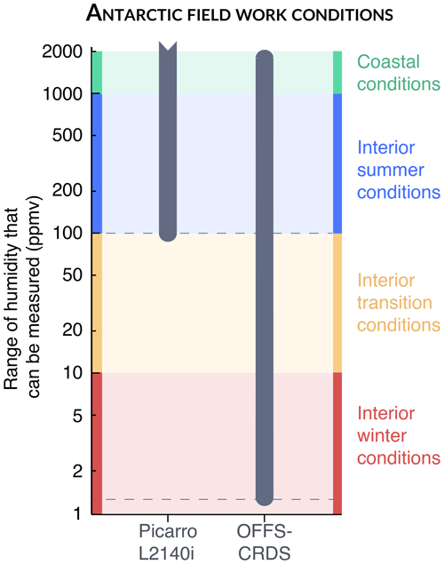
Figure 9Range of humidities at which the instrument can measure isotopic composition with a precision better than 1 ‰.
One limitation to determine the true precision and accuracy of the VCOF-CRDS instrument comes from the vapour generation from either the dedicated instrument (Leroy-Dos Santos et al., 2021) or the outgassing of the tubes. Indeed, at such low humidity, it is challenging to limit the variations in the humidity levels below 1 ppmv, which can account for a significant number of the total humidity levels below 100 ppmv. The use of several instruments monitoring the same water vapour would be needed to disentangle the various contributions to the variability coming from the water generation from the one coming from the measurement.
The current instrument cannot be deployed in the field due to its size and weight (1 m3, 230 kg), the fragility of the VCOF source (the glass cavity is suspended by fragile ceramic rods; vacuum must be maintained), and the bulkiness and the frailty of the control electronics (instruments must be extremely isolated for static shocks due to the lack of electric grounding with the thick ice layer). The performance of the instrument in the field should be roughly the same, provided that the temperature stabilisation of the instrument is as good as in the air-conditioned rooms of the lab. Indeed, the proof of concept for the frequency auto-referencing shows that the instrument will not suffer drift associated with change in the laser source wavelength. Another caveat before the instrument can be deployed for fieldwork is to take into account interferences from other species. For instance, taking into account the impact of methane absorption features at 7199.95 and 7200.03 cm−1 will require adding an extra spectral point for Antarctic field study as the methane absorption should be as strong as the water ones at humidity levels around 1 ppmv, following a similar approach to Chaillot et al. (2023).
The determination of physical parameters associated with the different heavy isotopes is also limited by instrumental capabilities. Currently, several studies attempted to measure the fractionation associated with gaseous-to-solid phase transitions and ended with contradictory results at temperatures below −30 °C (Ellehoj et al., 2013; Lamb et al., 2017; Majoube, 1971). Better determinations of these fractionation coefficients are key for isotope-enabled climate models (Risi et al., 2008; Werner et al., 2011) which use these parameterisations throughout the water cycle, with temperatures often much lower than −30 °C, especially in high-altitude cloud microphysics processes. Using dedicated laboratory experiments, the VCOF-CRDS instrument would be well suited to determine the equilibrium fractionation coefficient down to −80 °C, shedding light on fractionation processes at temperature ranges relevant for cloud microphysics or in polar regions.
We build an infrared spectrometer based on relatively cheap telecom components enhanced by the high performance of optical feedback frequency stabilisation and cavity ring-down spectroscopy. This instrument demonstrates a precision and a stability of 0.01 ‰ for δ18O and 0.1 ‰ for d-excess at extremely low humidities such as those found in central Antarctica for durations longer than 2 d. A key element to ensure limited drift even outside of the confine of a fully equipped spectroscopy lab is the use of the Lamb-dip feature as a frequency reference. This shows that the instrument is able to reach the same level of precision without any external validation of the frequency of the laser source. While this instrument cannot be transported to Antarctica, by supporting measurement down to 1 ppmv of humidity, this technique shows great potential to study the isotopic exchanges all year long in Antarctica where temperature can reach −80 °C during the polar night.
The humidity generator used here is based on the instrument described in Leroy-Dos Santos et al. (2021). The humidity levels it generates, while extremely stable, are limited to a stability of roughly 20 ppmv over 1 h. Due to the high precision of the infrared spectrometer discussed in this paper, it is possible that the drift observed on the isotopic composition here is linked to instability in the generated water humidity and thus the isotopic composition associated with limited variations in the water and air inflow in the humidity generator. Figure A1a shows the variations in humidity over the 8 d period that were used to produce the Allan standard deviation curve at 400 ppmv in Fig. 4a. Over the course of 8 d, the measured humidity only varied by 10 ppmv, principally during the refill of the syringe of the humidity generator (Leroy-Dos Santos et al., 2021). In addition, a drift of roughly 2.5 ppmv over the 8 d is visible on the time series. This drift is clearly visible in the Allan standard deviation plots (Fig. A1b). The shape of the increase in the Allan standard deviation of specific humidity around 1 h is very similar to the bump in the δ18O Allan standard deviation (Fig. 4a), which suggests that the instability in the generated vapour sample could have created excess noise which is not linked to the spectrometer.
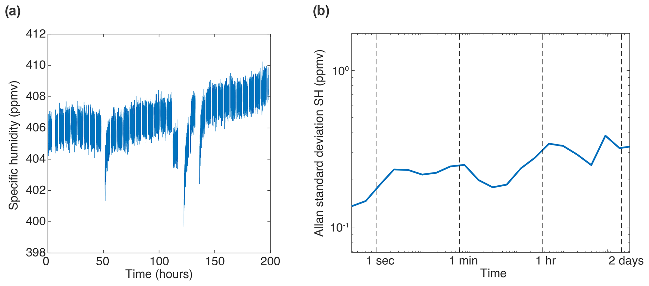
Figure A1(a) Specific humidity time series during an 8 d monitoring of a stable isotopic sample. (b) Allan standard deviation plots of the specific humidity (SH) measurements.
Figure 4 and the Results section focus on δ18O and d-excess because of the excess noise found in the δ18O measurements due to the misalignment of the measurement point off the centre of the O transition. In fact, we expect the drift of d-excess to be dominated by the drift of δ18O due to the excess noise. Here, we show that this is relatively true at short timescales (below 1 h; Fig. B1). At longer timescales, the excess noise from δD leads to a flat response of the d-excess Allan standard deviation.
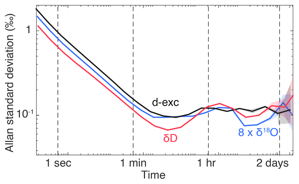
Figure B1Comparison of the Allan standard deviations of δ18O (scaled by a factor of 8 to ease the comparison), δD, and d-excess realised at 400 ppmv.
The code to compute Allan variance from datasets including NaNs is available at https://github.com/MathieuIso/Glaciotools/tree/389ba1344443be17af20859ed7f22f73c0dedad4/nanavar (https://doi.org/10.5281/zenodo.13235227, Casado, 2024). This code has been developed by Mathieu Casado, Thomas Lauwers, and Louis Wieczorek in MATLAB and Python and will be maintained as bugs are identified.
No datasets were used in this article.
AL and SK organised the project. MC, TS, JC, and SK built the instrument. FP and BB supported the project and the measurements. MC wrote the manuscript with the help of all the co-authors.
The contact author has declared that none of the authors has any competing interests.
Publisher's note: Copernicus Publications remains neutral with regard to jurisdictional claims made in the text, published maps, institutional affiliations, or any other geographical representation in this paper. While Copernicus Publications makes every effort to include appropriate place names, the final responsibility lies with the authors.
The research leading to these results has received funding from the European Research Council COMBINISO project (FP7/2007-2013) grant agreement number 306045 and SAMIR project (HORIZON) grant agreement number 101116660. We thank Erik Kerstel, Daniele Romanini, Johannes Burkart, and Peter Cermak for our fruitful discussions which helped improve the manuscript. We would like to thank the editor, Pierre Herckes, and the four anonymous reviewers and reviewer Béla Tuzson for their comments which improved the quality of the manuscript.
This research has been supported by the European Research Council (FP7 Ideas: European Research Council, grant no. 306045; HORIZON: European Research Council, grant no. 101116660). In addition, funding from the CNRS MITI project MILES has supported this study.
This paper was edited by Pierre Herckes and reviewed by Béla Tuzson and four anonymous referees.
Akers, P. D., Kopec, B. G., Mattingly, K. S., Klein, E. S., Causey, D., and Welker, J. M.: Baffin Bay sea ice extent and synoptic moisture transport drive water vapor isotope (δ18O, δ2H, and deuterium excess) variability in coastal northwest Greenland, Atmos. Chem. Phys., 20, 13929–13955, https://doi.org/10.5194/acp-20-13929-2020, 2020.
Bagheri Dastgerdi, S., Behrens, M., Bonne, J.-L., Hörhold, M., Lohmann, G., Schlosser, E., and Werner, M.: Continuous monitoring of surface water vapour isotopic compositions at Neumayer Station III, East Antarctica, The Cryosphere, 15, 4745–4767, https://doi.org/10.5194/tc-15-4745-2021, 2021.
Berkelhammer, M., Noone, D. C., Steen-Larsen, H. C., Bailey, A., Cox, C. J., O'Neill, M. S., Schneider, D., Steffen, K., and White, J. W. C.: Surface-atmosphere decoupling limits accumulation at Summit, Greenland, Sci. Adv., 2, e1501704, https://doi.org/10.1126/sciadv.1501704, 2016.
Bonne, J.-L., Masson-Delmotte, V., Cattani, O., Delmotte, M., Risi, C., Sodemann, H., and Steen-Larsen, H. C.: The isotopic composition of water vapour and precipitation in Ivittuut, southern Greenland, Atmos. Chem. Phys., 14, 4419–4439, https://doi.org/10.5194/acp-14-4419-2014, 2014.
Bonne, J.-L., Behrens, M., Meyer, H., Kipfstuhl, S., Rabe, B., Schönicke, L., Steen-Larsen, H. C., and Werner, M.: Resolving the controls of water vapour isotopes in the Atlantic sector, Nat. Commun., 10, 1–10, 2019.
Bréant, C., Dos Santos, C. L., Agosta, C., Casado, M., Fourré, E., Goursaud, S., Masson-Delmotte, V., Favier, V., Cattani, O., and Prié, F.: Coastal water vapor isotopic composition driven by katabatic wind variability in summer at Dumont d'Urville, coastal East Antarctica, Earth Planet. Sc. Lett., 514, 37–47, 2019.
Burkart, J. and Kassi, S.: Absorption line metrology by optical feedback frequency-stabilized cavity ring-down spectroscopy, Appl. Phys. B, 119, 97–109, https://doi.org/10.1007/s00340-014-5999-3, 2015.
Burkart, J., Romanini, D., and Kassi, S.: Optical feedback stabilized laser tuned by single-sideband modulation, Opt. Lett., 38, 2062–2064, 2013.
Burkart, J., Romanini, D., and Kassi, S.: Optical feedback frequency stabilized cavity ring-down spectroscopy, Opt. Lett., 39, 4695–4698, https://doi.org/10.1364/OL.39.004695, 2014.
Burkart, J., Sala, T., Romanini, D., Marangoni, M., Campargue, A., and Kassi, S.: Communication: Saturated CO2 absorption near 1.6 µm for kilohertz-accuracy transition frequencies, J. Chem. Phys., 142, 191103, https://doi.org/10.1063/1.4921557, 2015.
Casado, M.: Water stable isotopic composition on the East Antarctic Plateau: measurements at low temperature of the vapour composition, utilisation as an atmospheric tracer and implication for paleoclimate studies, PhD Thesis, Paris Saclay, https://theses.hal.science/tel-01409702 (last access: 6 August 2024), 2016.
Casado, M.: Antarctic Stable Isotopes, in: Reference Module in Earth Systems and Environmental Sciences, online Reference Collection, Elsevier, ISBN 9780124095489, 2018.
Casado, M.: MathieuIso/Glaciotools: Glaciotools (Version v1), Zenodo [code], https://doi.org/10.5281/zenodo.13235227, 2024.
Casado, M., Landais, A., Masson-Delmotte, V., Genthon, C., Kerstel, E., Kassi, S., Arnaud, L., Picard, G., Prie, F., Cattani, O., Steen-Larsen, H.-C., Vignon, E., and Cermak, P.: Continuous measurements of isotopic composition of water vapour on the East Antarctic Plateau, Atmos. Chem. Phys., 16, 8521–8538, https://doi.org/10.5194/acp-16-8521-2016, 2016.
Casado, M., Landais, A., Picard, G., Münch, T., Laepple, T., Stenni, B., Dreossi, G., Ekaykin, A., Arnaud, L., Genthon, C., Touzeau, A., Masson-Delmotte, V., and Jouzel, J.: Archival processes of the water stable isotope signal in East Antarctic ice cores, The Cryosphere, 12, 1745–1766, https://doi.org/10.5194/tc-12-1745-2018, 2018.
Casado, M., Münch, T., and Laepple, T.: Climatic information archived in ice cores: impact of intermittency and diffusion on the recorded isotopic signal in Antarctica, Clim. Past, 16, 1581–1598, https://doi.org/10.5194/cp-16-1581-2020, 2020.
Casado, M., Landais, A., Picard, G., Arnaud, L., Dreossi, G., Stenni, B., and Prié, F.: Water isotopic signature of surface snow metamorphism in Antarctica, Geophys. Res. Lett., 48, e2021GL093382, https://doi.org/10.1029/2021GL093382, 2021.
Casado, M., Stoltmann, T., Landais, A., Jobert, N., Daëron, M., Prié, F., and Kassi, S.: High stability in near-infrared spectroscopy: part 1, adapting clock techniques to optical feedback, Appl. Phys. B, 128, 1–7, 2022.
Čermák, P., Karlovets, E. V, Mondelain, D., Kassi, S., Perevalov, V. I., and Campargue, A.: High sensitivity CRDS of CO2 in the 1.74 µm transparency window. A validation test for the spectroscopic databases, J. Quant. Spectrosc. Ra., 207, 95–103, 2018.
Chaillot, J., Dasari, S., Fleurbaey, H., Daeron, M., Savarino, J., and Kassi, S.: High-precision laser spectroscopy of H2S for simultaneous probing of multiple-sulfur isotopes, Environ. Sci. Adv., 2, 78–86, https://doi.org/10.1039/D2VA00104G, 2023.
Craig, H. and Gordon, L. I.: Deuterium and oxygen-18 variations in the ocean and the marine atmosphere, in: Stable Isotopes in Oceanographic Studies and Palaiotemperatures, edited by: Tongiorgi, E., Lab. Geol. Nucl. Pisa, Italy, 1–122, 1965.
Dansgaard, W.: Stable isotopes in precipitation, Tellus, 16, 436–468, https://doi.org/10.1111/j.2153-3490.1964.tb00181.x, 1964.
Ekaykin, A. A., Lipenkov, V. Y., Barkov, N. I., Petit, J. R., and Masson-Delmotte, V.: Spatial and temporal variability in isotope composition of recent snow in the vicinity of Vostok station, Antarctica: implications for ice-core record interpretation, Ann. Glaciol., 35, 181–186, https://doi.org/10.3189/172756402781816726, 2002.
Ellehoj, M. D., Steen-Larsen, H. C., Johnsen, S. J., and Madsen, M. B.: Ice-vapor equilibrium fractionation factor of hydrogen and oxygen isotopes: Experimental investigations and implications for stable water isotope studies, Rapid Commun. Mass Sp., 27, 2149–2158, https://doi.org/10.1002/rcm.6668, 2013.
EPICA: Eight glacial cycles from an Antarctic ice core, Nature, 429, 623–628, https://doi.org/10.1038/nature02599, 2004.
Galewsky, J., Steen-Larsen, H. C., Field, R. D., Worden, J., Risi, C., and Schneider, M.: Stable isotopes in atmospheric water vapor and applications to the hydrologic cycle, Rev. Geophys., 54, 809–865, 2016.
Genthon, C., Piard, L., Vignon, E., Madeleine, J.-B., Casado, M., and Gallée, H.: Atmospheric moisture supersaturation in the near-surface atmosphere at Dome C, Antarctic Plateau, Atmos. Chem. Phys., 17, 691–704, https://doi.org/10.5194/acp-17-691-2017, 2017.
Genthon, C., Veron, D., Vignon, E., Six, D., Dufresne, J.-L., Madeleine, J.-B., Sultan, E., and Forget, F.: 10 years of temperature and wind observation on a 45 m tower at Dome C, East Antarctic plateau, Earth Syst. Sci. Data, 13, 5731–5746, https://doi.org/10.5194/essd-13-5731-2021, 2021.
Genthon, C., Veron, D. E., Vignon, E., Madeleine, J.-B., and Piard, L.: Water vapor in cold and clean atmosphere: a 3-year data set in the boundary layer of Dome C, East Antarctic Plateau, Earth Syst. Sci. Data, 14, 1571–1580, https://doi.org/10.5194/essd-14-1571-2022, 2022.
Gotti, R., Sala, T., Prevedelli, M., Kassi, S., Marangoni, M., and Romanini, D.: Feed-forward comb-assisted coherence transfer to a widely tunable DFB diode laser, J. Chem. Phys., 149, 154201, https://doi.org/10.1063/1.5046387, 2018.
Izutsu, M., Shikama, S., and Sueta, T.: Integrated optical SSB modulator/frequency shifter, IEEE J. Quantum Elect., 17, 2225–2227, 1981.
Jobert, N., Casado, M., and Kassi, S.: High stability in near-infrared spectroscopy: part 2, optomechanical analysis of an optical contacted V-shaped cavity, Appl. Phys. B, 128, 56, https://doi.org/10.1007/s00340-022-07779-x, 2022.
Jouzel, J. and Masson-Delmotte, V.: Paleoclimates: what do we learn from deep ice cores?, WIREs Clim. Change, 1, 654–669, https://doi.org/10.1002/wcc.72, 2010.
Kassi, S., Stoltmann, T., Casado, M., Daëron, M., and Campargue, A.: Lamb dip CRDS of highly saturated transitions of water near 1.4 µm, J. Chem. Phys., 148, 54201, https://doi.org/10.1063/1.5010957, 2018.
Kurita, N., Hirasawa, N., Koga, S., Matsushita, J., and Fujiyoshi, Y.: Identification of Air Masses Responsible for Warm Events on the East Antarctic Coast, SOLA, 12, 307–313, https://doi.org/10.2151/sola.2016-060, 2016.
Laepple, T., Münch, T., Casado, M., Hoerhold, M., Landais, A., and Kipfstuhl, S.: On the similarity and apparent cycles of isotopic variations in East Antarctic snow pits, The Cryosphere, 12, 169–187, https://doi.org/10.5194/tc-12-169-2018, 2018.
Lamb, K. D., Clouser, B. W., Bolot, M., Sarkozy, L., Ebert, V., Saathoff, H., Möhler, O., and Moyer, E. J.: Laboratory measurements of isotopic fractionation during ice deposition in simulated cirrus clouds, P. Natl. Acad. Sci. USA, 114, 5612–5617, 2017.
Landsberg, J., Romanini, D., and Kerstel, E.: Very high finesse optical-feedback cavity-enhanced absorption spectrometer for low concentration water vapor isotope analyses, Opt. Lett., 39, 1795–1798, https://doi.org/10.1364/OL.39.001795, 2014.
Laurent, P., Clairon, A., and Breant, C.: Frequency noise analysis of optically self-locked diode lasers, Quantum Electron. IEEE J., 25, 1131–1142, 1989.
Leroy-Dos Santos, C., Masson-Delmotte, V., Casado, M., Fourré, E., Steen-Larsen, H. C., Maturilli, M., Orsi, A., Berchet, A., Cattani, O., and Minster, B.: A 4.5 year-long record of Svalbard water vapor isotopic composition documents winter air mass origin, J. Geophys. Res.-Atmos., 125, e2020JD032681, https://doi.org/10.1029/2020JD032681, 2020.
Leroy-Dos Santos, C., Casado, M., Prié, F., Jossoud, O., Kerstel, E., Farradèche, M., Kassi, S., Fourré, E., and Landais, A.: A dedicated robust instrument for water vapor generation at low humidity for use with a laser water isotope analyzer in cold and dry polar regions, Atmos. Meas. Tech., 14, 2907–2918, https://doi.org/10.5194/amt-14-2907-2021, 2021.
Long, D. A., Bielska, K., Lisak, D., Havey, D. K., Okumura, M., Miller, C. E., and Hodges, J. T.: The air-broadened, near-infrared CO2 line shape in the spectrally isolated regime: Evidence of simultaneous Dicke narrowing and speed dependence, J. Chem. Phys., 135, 064308, https://doi.org/10.1063/1.3624527, 2011.
Lorius, C., Merlivat, L., and Hagemann, R.: Variation in the mean deuterium content of precipitations in Antarctica, J. Geophys. Res., 74, 7027–7031, https://doi.org/10.1029/JC074i028p07027, 1969.
Majoube, M.: FRACTIONATION IN O-18 BETWEEN ICE AND WATER VAPOR, J. Chim. Phys. P. C. B., 68, 625–636, 1971.
Merlivat, L. and Nief, G.: Fractionnement isotopique lors des changements d'état solide-vapeur et liquide-vapeur de l'eau à des températures inférieures à 0 °C, Tellus, 19, 122–127, https://doi.org/10.1111/j.2153-3490.1967.tb01465.x, 1967.
Morville, J., Kassi, S., Chenevier, M., and Romanini, D.: Fast, low-noise, mode-by-mode, cavity-enhanced absorption spectroscopy by diode-laser self-locking, Appl. Phys. B, 80, 1027–1038, https://doi.org/10.1007/s00340-005-1828-z, 2005.
North Greenland Ice Core Project members: High-resolution record of Northern Hemisphere climate extending into the last interglacial period, Nature, 431, 147–151, https://doi.org/10.1038/nature02805, 2004.
Risi, C., Bony, S., and Vimeux, F.: Influence of convective processes on the isotopic composition (δ18O and δD) of precipitation and water vapor in the tropics: 2. Physical interpretation of the amount effect, J. Geophys. Res.-Atmos., 113, D19306, https://doi.org/10.1029/2008JD009943, 2008.
Ritter, F., Steen-Larsen, H. C., Werner, M., Masson-Delmotte, V., Orsi, A., Behrens, M., Birnbaum, G., Freitag, J., Risi, C., and Kipfstuhl, S.: Isotopic exchange on the diurnal scale between near-surface snow and lower atmospheric water vapor at Kohnen station, East Antarctica, The Cryosphere, 10, 1647–1663, https://doi.org/10.5194/tc-10-1647-2016, 2016.
Romanini, D., Kachanov, A. A., Sadeghi, N., and Stoeckel, F.: CW cavity ring down spectroscopy, Chem. Phys. Lett., 264, 316–322, https://doi.org/10.1016/S0009-2614(96)01351-6, 1997.
Steen-Larsen, H. C., Johnsen, S. J., Masson-Delmotte, V., Stenni, B., Risi, C., Sodemann, H., Balslev-Clausen, D., Blunier, T., Dahl-Jensen, D., Ellehøj, M. D., Falourd, S., Grindsted, A., Gkinis, V., Jouzel, J., Popp, T., Sheldon, S., Simonsen, S. B., Sjolte, J., Steffensen, J. P., Sperlich, P., Sveinbjörnsdóttir, A. E., Vinther, B. M., and White, J. W. C.: Continuous monitoring of summer surface water vapor isotopic composition above the Greenland Ice Sheet, Atmos. Chem. Phys., 13, 4815–4828, https://doi.org/10.5194/acp-13-4815-2013, 2013.
Steen-Larsen, H. C., Masson-Delmotte, V., Hirabayashi, M., Winkler, R., Satow, K., Prié, F., Bayou, N., Brun, E., Cuffey, K. M., Dahl-Jensen, D., Dumont, M., Guillevic, M., Kipfstuhl, S., Landais, A., Popp, T., Risi, C., Steffen, K., Stenni, B., and Sveinbjörnsdottír, A. E.: What controls the isotopic composition of Greenland surface snow?, Clim. Past, 10, 377–392, https://doi.org/10.5194/cp-10-377-2014, 2014.
Steig, E. J., Gkinis, V., Schauer, A. J., Schoenemann, S. W., Samek, K., Hoffnagle, J., Dennis, K. J., and Tan, S. M.: Calibrated high-precision 17O-excess measurements using cavity ring-down spectroscopy with laser-current-tuned cavity resonance, Atmos. Meas. Tech., 7, 2421–2435, https://doi.org/10.5194/amt-7-2421-2014, 2014.
Stoltmann, T., Casado, M., Daëron, M., Landais, A., and Kassi, S.: Direct, Precise Measurements of Isotopologue Abundance Ratios in CO2 Using Molecular Absorption Spectroscopy: Application to Δ17O, Anal. Chem., 89, 10129–10132, 2017.
Thurnherr, I., Kozachek, A., Graf, P., Weng, Y., Bolshiyanov, D., Landwehr, S., Pfahl, S., Schmale, J., Sodemann, H., Steen-Larsen, H. C., Toffoli, A., Wernli, H., and Aemisegger, F.: Meridional and vertical variations of the water vapour isotopic composition in the marine boundary layer over the Atlantic and Southern Ocean, Atmos. Chem. Phys., 20, 5811–5835, https://doi.org/10.5194/acp-20-5811-2020, 2020.
Wei, Z., Lee, X., Aemisegger, F., Benetti, M., Berkelhammer, M., Casado, M., Caylor, K., Christner, E., Dyroff, C., and García, O.: A global database of water vapor isotopes measured with high temporal resolution infrared laser spectroscopy, Sci. Data, 6, 1–15, 2019.
Weng, Y., Touzeau, A., and Sodemann, H.: Correcting the impact of the isotope composition on the mixing ratio dependency of water vapour isotope measurements with cavity ring-down spectrometers, Atmos. Meas. Tech., 13, 3167–3190, https://doi.org/10.5194/amt-13-3167-2020, 2020.
Werner, M., Langebroek, P. M., Carlsen, T., Herold, M., and Lohmann, G.: Stable water isotopes in the ECHAM5 general circulation model: Toward high-resolution isotope modeling on a global scale, J. Geophys. Res.-Atmos., 116, D15109, https://doi.org/10.1029/2011JD015681, 2011.
- Abstract
- Introduction
- Methods and instrumental set-up
- Results
- Discussions
- Conclusion
- Appendix A: Evaluation of the stability of the generated vapour levels
- Appendix B: Comparison of the Allan standard deviation of δ18O and δD
- Code availability
- Data availability
- Author contributions
- Competing interests
- Disclaimer
- Acknowledgements
- Financial support
- Review statement
- References