Atmospheric H₂ observations from the NOAA Cooperative Global Air Sampling Network

The NOAA Global Monitoring Laboratory (GML) measures atmospheric hydrogen (H₂) in grab samples collected weekly as flask pairs at over 50 sites in the Cooperative Global Air Sampling Network. Measurements representative of background air sampling show higher H₂ in recent years at all latitudes. The marine boundary layer (MBL) global mean H₂ was 552.8 ppb in 2021, 20.2 ± 0.2 ppb higher compared to 2010. A 10 ppb or more increase over the 2010–2021 average annual cycle was detected in 2016 for MBL zonal means in the tropics and in the Southern Hemisphere. Carbon monoxide measurements in the same-air samples suggest large biomass burning events in different regions likely contributed to the observed interannual variability at different latitudes. The NOAA H₂ measurements from 2009 to 2021 are now based on the World Meteorological Organization Global Atmospheric Watch (WMO GAW) H₂ mole fraction calibration scale, developed and maintained by the Max Planck Institute for Biogeochemistry (MPI-BGC), Jena, Germany. GML maintains eight H₂ primary calibration standards to propagate the WMO scale. These are gravimetric hydrogen-in-air mixtures in electropolished stainless steel cylinders (Essex Industries, St. Louis, MO), which are stable for H₂. These mixtures were calibrated at the MPI-BGC, the WMO Central Calibration Laboratory (CCL) for H₂, in late 2020 and span the range 250–700 ppb. We have used the CCL assignments to propagate the WMO H₂ calibration scale to NOAA air measurements performed using gas chromatography and helium pulse discharge detector instruments since 2009. To propagate the scale, NOAA uses a hierarchy of secondary and tertiary standards, which consist of high-pressure whole-air mixtures in aluminum cylinders, calibrated against the primary and secondary standards, respectively. Hydrogen at the parts per billion level has a tendency to increase in aluminum cylinders over time. We fit the calibration histories of these standards with zero-, first-, or second-order polynomial functions of time and use the time-dependent mole fraction assignments on the WMO scale to reprocess all tank air and flask air H₂ measurement records. The robustness of the scale propagation over multiple years is evaluated with the regular analysis of target air cylinders and with long-term same-air measurement comparison efforts with WMO GAW partner laboratories. Long-term calibrated, globally distributed, and freely accessible measurements of H₂ and other gases and isotopes continue to be essential to track and interpret regional and global changes in the atmosphere composition. The adoption of the WMO H₂ calibration scale and subsequent reprocessing of NOAA atmospheric data constitute a significant improvement in the NOAA H₂ measurement records.

1 Introduction

High-quality and sustained observations are essential to track and study changes in atmospheric trace gas distributions. Ambient air measurement programs for trace gases provide objective data to track air pollution levels (Oltmans and Levy, 1994; Thompson et al., 2004; Tørseth et al., 2012; Schultz et al., 2015; Cooper et al., 2020; WMO, 2022) to study how a mix of sources (and sinks) impact the air composition (Ciais et al., 1995; Pétron et al., 2012; Langenfelds et al., 2002; Brito et al., 2015) and to constrain and evaluate fluxes and their trends at scales of interest (von Schneidemesser et al., 2010; Simpson et al., 2012; Propper et al., 2015; Montzka et al., 2018; Friedlingstein et al., 2022; Heiskanen et al., 2022; Storm et al., 2023).

H₂ is a trace gas in the Earth's atmosphere, and its abundance can indirectly impact climate and air quality. The analysis of H₂ measurements in firn air collected in Antarctica reveals that H₂ levels in the high-latitude Southern Hemisphere grew by some 70 % (330 to 550 ppb, 1 ppb = 1 mole of gas per billion (10⁹) moles of air) over the 20th century (Patterson et al., 2021, 2023). Greenland firn air covers less depth and time, but results are consistent with a 30 % increase in high-latitude Northern Hemisphere H₂ from 1950 to the late 1980s (Patterson et al., 2023). Growing emissions related to fossil fuel burning most likely were behind this rise in H₂ (Patterson et al., 2021). Results also show that H₂ in both polar regions leveled off after the 1990s (Patterson et al., 2021, 2023).

H₂ has been viewed as a potential low or zero carbon energy carrier for close to 5 decades (Yap and McLellan, 2023). Since 2020 there has been renewed interest in the hydrogen economy (Yap and McLellan, 2023) spurred by a rise in announcements of public and private projects to produce low-carbon H₂, also referred to as “blue” H₂ produced from natural gas with carbon capture, utilization, and storage, or “green” H₂ produced using renewable energy (Hydrogen Council and McKinsey & Company, 2023). In 2021, H₂ global demand was over 94×10⁶ t or 2.5 % of global final energy consumption (IEA, 2022). This demand was almost entirely driven by refineries and a few industries (ammonia, methanol, and steel), and H₂ production almost entirely relied on fossil fuels with unabated emissions (“gray H₂”; IEA, 2022). As of December 2023, over 1400 announced projects globally (worth USD 570 billion) are anticipated to increase the global H₂ production capacity by 45×10⁶ t through 2030 (Hydrogen Council and McKinsey & Company, 2023).

Studies of the potential short-term and long-term climate impacts of increased H₂ production and use have called for more research to better understand the current and future H₂ supply chain and end-use emissions of H₂ and greenhouse gases (GHGs) (Ocko and Hamburg, 2022; Longden et al., 2022; de Kleijne et al., 2022; Bertagni et al., 2022; Warwick et al., 2023). Global, high-quality, and sustained atmospheric measurements of H₂ can provide independent information to document its distribution and study its sources and sinks and how they may change.

The National Oceanic and Atmospheric Administration (NOAA) Cooperative Global Air Sampling Network comprises over 50 surface and mostly remote sites (https://gml.noaa.gov/ccgg/flask.html, last access: 17 July 2024). At each site and on a weekly basis, local partners collect air in two 2.5 L glass flasks and then return the flasks to the NOAA Global Monitoring Laboratory (GML) in Boulder, Colorado, USA, for measurements of major long-lived greenhouse gases, carbon dioxide (CO₂), methane (CH₄), nitrous oxide (N₂O), and sulfur hexafluoride (SF₆), as well as carbon monoxide (CO) and hydrogen (H₂) (Conway et al., 1994; Novelli et al., 1999; Dlugokencky et al., 2009). The network is a contributor to the World Meteorological Organization (WMO) Global Atmospheric Watch (GAW) program, which promotes and coordinates international scientific efforts and free access to long-term atmospheric observations (WMO, 2020).

CO and H₂ are important trace gases that share sources with CO₂ and CH₄ (fossil fuel burning, biofuel burning, and wildfires). Reaction with hydroxyl radicals (OH) is the main sink for CH₄ and CO and an important sink for H₂. Both H₂ and CO are also produced during the chemical oxidation of CH₄ and nonmethane hydrocarbons. Soil uptake by bacteria accounts for 75 % of the total H₂ sink. H₂ and CO have much shorter atmospheric lifetimes than CO₂ and CH₄: 2–3 months for CO and close to 2 years for H₂. The H₂ global mean atmospheric lifetime is largely driven by the soil sink strength. The H₂ lifetime related to the oxidation by OH is estimated to be 8–9 years (Price et al., 2007; Warwick et al., 2022).​​​​​​​

Novelli et al. (1991, 1992) reported for NOAA on testing the air sampling approach (flask type, stopcock fitting, wet or dry air, untaped vs. taped glass flasks to minimize direct sunlight exposure) and an analytical instrument consisting of a gas chromatograph (GC) and a reduction gas analyzer (RGA, from Trace Analytical Inc., California) that could measure both CO and H₂. Around that time, other laboratories had also adopted the technique for CO and H₂ measurements in discrete air samples or in situ. Khalil and Rasmussen (1989, 1990) reported on H₂ measurements of whole-air samples collected weekly in triplicate electropolished stainless steel flasks between October 1985 and April 1989 at the four NOAA atmospheric baseline observatories (Point Barrow, Mauna Loa, Samoa, South Pole); Cape Meares, Oregon; Cape Kumukahi, Hawaii; and the Kennaook/Cape Grim Observatory, Tasmania. These measurements showed that, contrary to CO₂, CH₄, N₂O, and CO, background air H₂ levels were higher in the Southern Hemisphere (SH) than in the Northern Hemisphere (NH). The 1985–1987 monthly mean observed H₂ ranged between 500–520 ppb at the South Pole and between 455 and 520 ppb at Point Barrow. H₂ exhibited a strong seasonal cycle at extratropical latitudes especially in the NH, and the seasonal cycles in both hemispheres were offset by 1–2 months only.

In 1995, H₂ mole fraction calibration standards were prepared gravimetrically in aluminum cylinders (Scott-Marrin Inc., Riverside, CA), and five of them (spanning 485–603 ppb) were used to define the NOAA H₂ X1996 calibration scale. Working standards used in the NOAA flask analysis laboratory between 1988 and 1996 were reassigned H₂ mole fractions, and flask air measurements were reprocessed to be on the X1996 scale. Novelli et al. (1999) described the early NOAA H₂ measurements and reported H₂ time series starting in the late 1980s or early 1990s (depending on the site) for 50 sites in the NOAA Cooperative Global Air Sampling Network.

Simmonds et al. (2000) reported in situ high-frequency GC–RGA measurements of H₂ at the Mace Head baseline atmospheric monitoring station on the Atlantic coast of Ireland for the 1994–1998 period. They found that the background air at Mace Head had lower monthly mean H₂ (470–520 ppb) than background air masses measured at the Kennaook/Cape Grim observatory (510–530 ppb) from July to April. Some of the 40 min H₂ observations showed 10–200 ppb short-term H₂ enhancements above baseline levels. The authors derived an estimate of European emissions with an inverse model of enhanced H₂ in air masses impacted by upwind sources of pollution. They also observed that nighttime measurements in low-wind conditions reflected local depletion of H₂. The authors derived variable mean deposition velocities and found that the H₂ soil sink was likely a process that occurred year-round in the area.

After 1996 and until 2008, the NOAA H₂ measurement program used successive working standards that were assigned based on GC–RGA measurements against the previous standards. With hindsight, the NOAA X1996 calibration scale transfer and the early NOAA H₂ measurements had several limitations which are briefly described below and in more detail in Sect. S1 in the Supplement.

By the late 1990s, same-air or colocated air sample measurement comparison between NOAA and the Commonwealth Scientific and Industrial Research Organisation (CSIRO) for the Kennaook/Cape Grim Observatory and Alert, Canada, flask air analyses showed an increasing bias for H₂ between the two laboratories (Masarie et al., 2001; Francey et al., 2003). Further laboratory tests by several WMO GAW measurement laboratories revealed the RGA detector response was nonlinear and required frequent calibration. Additionally measurement laboratories found that the H₂ mole fraction for air standards, especially those stored in high-pressure aluminum cylinders, could drift at rates of a few parts per billion (ppb) to tens of parts per billion per year (Novelli et al., 1999; Masarie et al., 2001; Jordan and Steinberg, 2011).

To address these compounding issues, in 2008 NOAA GML tested a new analytical instrument: a gas chromatograph with a pulse discharge helium ionization detector (GC-HePDD) (Wentworth et al., 1994). The technique showed very good performance with a stable and linear response over the 0–2000 ppb range, and it was adopted for the calibration scale propagation and flask air analysis of H₂ in 2009 (Novelli et al., 2009). Around that time GML also began testing electropolished stainless steel cylinders (Essex Industries, St. Louis, MO) filled with dry air for stability.

In 2007–2008, GML prepared six new gravimetric air mixtures in electropolished stainless steel cylinders spanning 250–600 ppb H₂. At that time, the new gravimetric mixtures differed by about +20 ppb compared to two H₂ secondary-standard values assigned on the NOAA H₂ X1996 scale. For the next decade, GML kept using the NOAA X1996 calibration scale while also conducting routine measurements of the H₂ secondary standards against the 2007 and 2008 gravimetric mixtures.

The GC-HePDD H₂ measurements on the NOAA H₂ X1996 scale remained biased compared to GAW partner measurements, and the NOAA H₂ data from the global network flasks were not released publicly after 2005. Sections S1–S3 and Table S1 provide additional information on issues impacting the 1988–2008 NOAA H₂ measurements on RGAs and related information from the CSIRO and Max Planck Institute for Biogeochemistry (MPI-BGC) H₂ measurement programs. The more precise and better-calibrated NOAA H₂ measurement records date back to 2009 and 2010 and are the main focus of this paper.

In fall 2020, GML initiated an effort to (1) adopt the WMO MPI X2009 H₂ calibration scale (Jordan and Steinberg, 2011) for future measurements and (2) convert GML H₂ measurements made on GC-HePDD instruments (beginning in late 2009) to that scale. This paper describes the MPI X2009 H₂ calibration scale propagation within GML and the revised measurements from the NOAA Cooperative Global Air Sampling Network flask air samples analyzed since late 2009. We show very good agreement for the reprocessed NOAA H₂ data for different WMO GAW measurement comparison efforts. The revised measurement records of NOAA GML flask air H₂ dry air mole fraction for over 50 surface sites from 2009–2021 are publicly available (Pétron et al., 2023a). This new dataset complements other WMO GAW H₂ measurement datasets and provides reliable observational constraints for the study of atmospheric H₂ global distribution and budget from 2009 onwards. Future NOAA H₂ dataset updates will be released as we use continued calibration results to reliably track the drift in standards and revise their assignments.

2 Adoption of the WMO MPI X2009 H₂ calibration scale

To infer fluxes and trends from atmospheric measurements, scientists need to reliably detect small temporal and spatial gradients in the abundance of trace gases. This requires comparable data across time and across monitoring networks to ensure biases are minimized and do not influence interpretation. The use of a common calibration scale among measurement laboratories ensures data are traceable to a common reference. It is the first step in preventing biases that could stem from using different references.

In this section, we introduce the NOAA GML H₂ calibration standard hierarchy and describe the adoption of the WMO MPI X2009 H₂ scale. The calibration at GML is based on a hierarchy of standards (primary, secondary, tertiary) and a dedicated H₂ calibration system used to transfer the scale from the primary standards to secondary and tertiary standards. An important quality assurance procedure within GML is the routine measurement of dedicated quality control cylinders (referred to as “target” tanks) to track instrument performance. Results are discussed in relation to the uncertainty of the flask air analysis systems and consistency of the MPI X2009 H₂ scale implementation.

2.1 NOAA GML H₂ primary standards

In 2007–2008, six mixtures of H₂ in dry air were prepared gravimetrically at GML in 34 L electropolished stainless steel cylinders (Novelli et al., 2009, and Table 1). The highest H₂ mole fraction tank developed a leak and was lost. The remaining set of five standards covered the range 250 to 600 ppb for H₂. Three standards in electropolished stainless steel cylinders were added in 2019 to extend the upper limit of the calibration range to 700 ppb H₂ and evaluate the stability of the initial set over the intervening years. In 2020, these eight standards were designated as NOAA GML's highest-level H₂ standards. We refer to them as the NOAA H₂ primary standards throughout this paper even though they are not used to independently define the scale.

Table 1 NOAA GML H₂ primary standards (prepared gravimetrically) and their WMO MPI X2009 assignments (dated 9 December 2020). All H₂ dry air mole fractions and their uncertainties are in parts per billion.

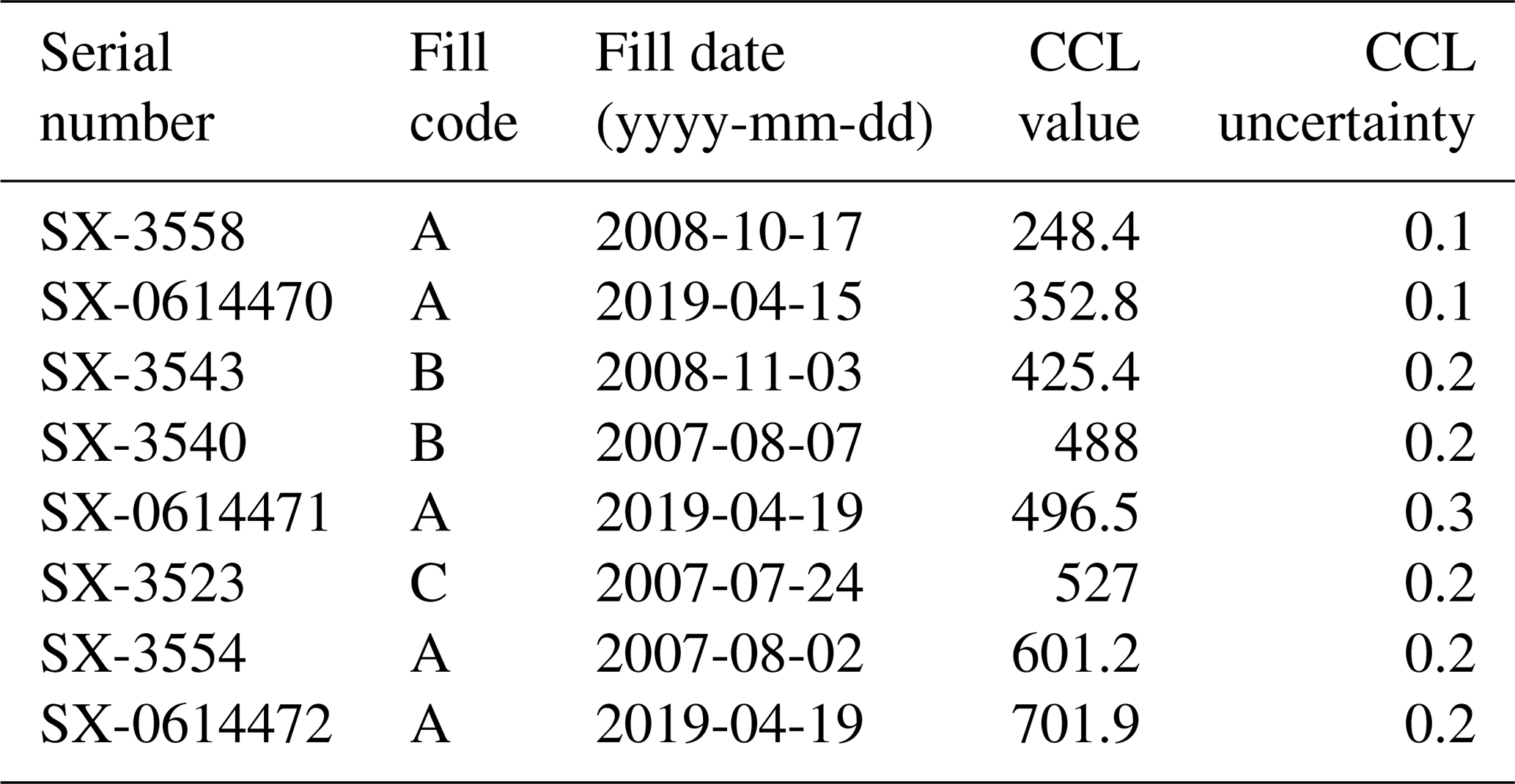
The eight primary standards were analyzed by the WMO Central Calibration Laboratory (CCL) for H₂ hosted by the MPI-BGC in Jena, Germany, on their GC-PDD system in November 2020. The results listed in Table 1 are reported on the MPI X2009 H₂ calibration scale (Jordan and Steinberg, 2011). The CCL uncertainty estimates listed in Table 1 refer to the standard deviation of the 25–32 discrete H₂ measurements made for each standard. Until they are recalibrated by the CCL, we add a 0.5 ppb 1σ uncertainty to these assignments. This is the currently reported CCL reproducibility for their GC-PDD H₂ measurements. It accounts for potential longer-term uncertainty in calibration results that would not be evident in the standard deviations of measurements made close in time.

2.2 MPI X2009 H₂ calibration scale transfer

GML has separate, dedicated analytical systems for scale propagation and flask air analyses. Novelli et al. (2009) describe the GC-HePDD instruments and the operating parameters in detail. GML has used three GC-HePDD instruments so far. Each is identified by a unique internal instrument identification code: H9 for tank calibrations and H8 and H11 for flask analyses. The GC-HePDD instruments' responses are linear (within 0.3 %) up to 2000 ppb. They are configured for parts-per-billion-level sensitivity and calibrated over the 200–700 ppb range, which is optimal for global and regional background air analysis.

The GML H₂ primary standards are used to periodically calibrate the H9 instrument response for the analysis and value assignment of lower-level standards. The stability and longevity of the primary standards are critical to ensure the consistency of the GML H₂ measurements over long periods of time required for trend analysis.

The H₂ secondary and tertiary standards used in GML are whole-air mixtures in high-pressure aluminum cylinders (Luxfer USA). Most were filled at the GML standard air preparation facility at the Niwot Ridge mountain research station using a RIX Industries (Benicia, CA) SA6 oil-free compressor (Kitzis, 2017). Two additional tertiary standards were purchased from Scott-Marrin. All GML tank air mixtures have a unique combination of an alphanumeric cylinder ID and a fill code letter (A–Z) tied to a fill date.

Aluminum tanks are known to be unstable for storing H₂ for air standards (Jordan and Steinberg, 2011). Therefore regular analyses of standards on the tank calibration system are critical for quantifying drift to allow a time-dependent value assignment on the MPI X2009 H₂ calibration scale.

GML uses Python software developed in-house to record calibration data, compute mole fractions, and evaluate the stability of H₂ mole fractions over time. All mole fraction assignments and associated drift coefficients for standards used to propagate a calibration scale are stored in a database table that can be accessed by the data processing software. The software allows for zero-, first-, or second-order polynomial drift functions. As new calibration results are available, the drift correction and assignment for a particular tank ID and fill code are revised as needed and the affected data are reprocessed.

2.2.1 Scale transfer: 2009–2019

From 2007 through mid-April 2019, the H₂ tank air calibration on the H9 instrument was conducted using a single standard gas (primary or secondary standard) to calibrate the “unknown” (secondary or tertiary) standards. A tank calibration event consisted of alternating injections of the standard gas and the unknown tank air with typically seven or more unknown air injections. The first aliquot in a multi-injection measurement sequence on H9 is often slightly biased (due to subtle timing differences with the regulator flush cycle) and is not used. The ratio of the H₂ peak height for each valid unknown air injection and the mean peak height of two bracketing standard gas injections (or sometimes only one preceding or following standard gas injection) is multiplied by the known H₂ mole fraction of the standard gas to calculate the unknown air injection mole fraction. Results for a tank air calibration event are defined by the mean and the standard deviation of the calculated H₂ mole fractions for five or more retained unknown air injections. Typically, the standard deviation for a tank air calibration event on H9 is less than 1 ppb.

Prior to the 2023 GML H₂ data reprocessing, GML used peak area for the GC-HePDD as described in Novelli et al. (1999). However, we saw that for some helium carrier gas tanks (Airgas Ultra High Purity, 99.999 % purity), the H₂ chromatogram peak had a tail or a noisy baseline. Since the H₂ peak height was less affected, we use peak height ratios for all GC-HePDD measurements. In 2023, GML switched to Matheson research-grade helium carrier gas for the GC-HePDDs (99.9999 % purity).

The calibration results for the two H₂ secondary standards used between 2009 and April 2019 are plotted in Fig. 1, and final assignments are listed in Table S2. A small non-zero y intercept for H9 (see next section) likely explains the biased results for CC119811 against the lowest primary standards (SX-3558 and SX-3543). Results against SX-3558 were not used for value-assigning any secondary standards, and results against SX-3543 were not used for CC119811.

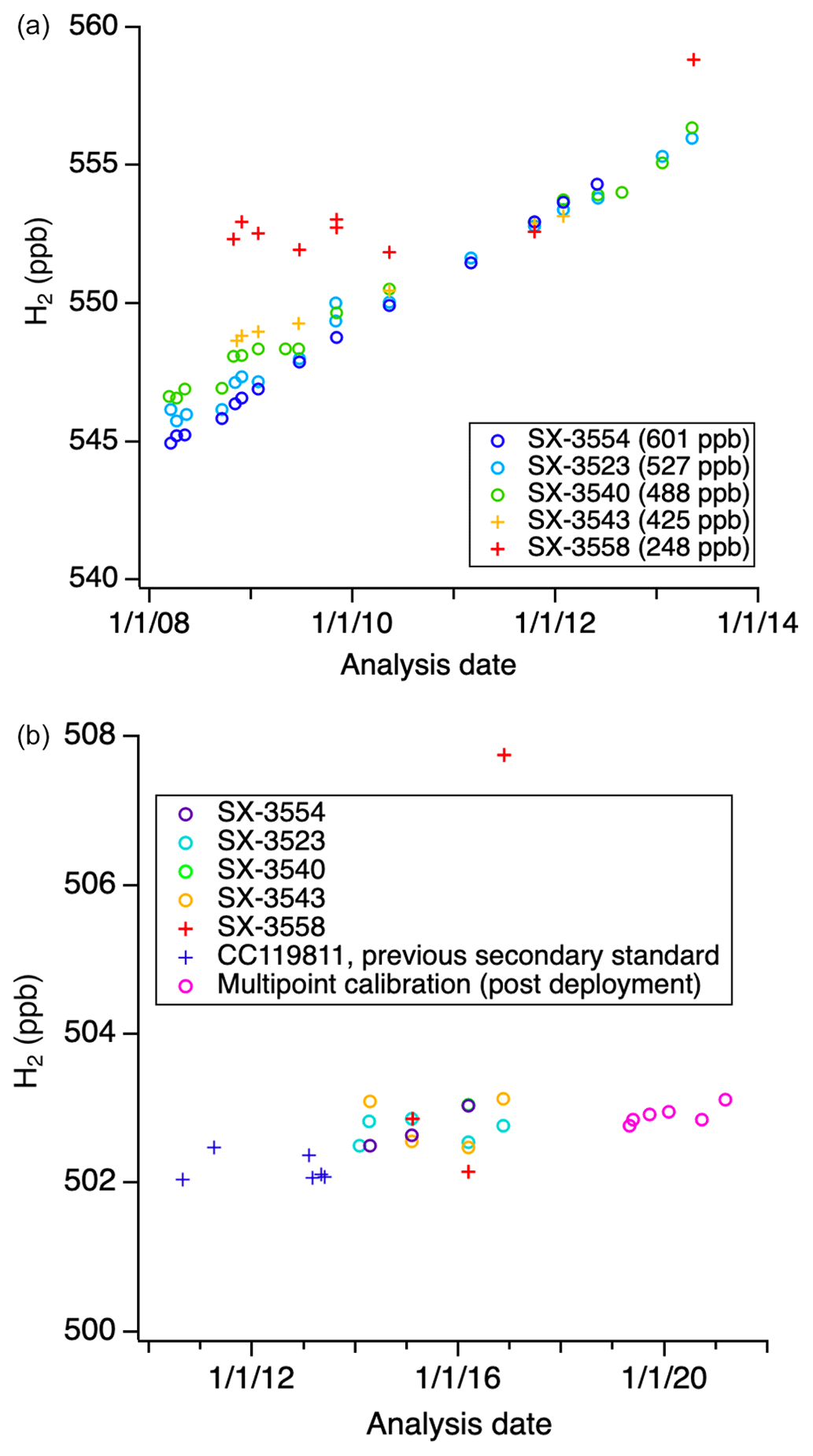
Figure 1 Calibration results for the two GML H₂ secondary standards (a) CC119811 and (b) CA03233 on H9 against one of the primary standards. The 2019–2020 multipoint calibration results on H9 are also shown for CA03233 (pink circles). Only results shown with open circles are used for the assignments.

CA03233 was stable for H₂ over its time of use and has an assignment of 502.8 ppb H₂. H₂ in CC119811 exhibited a small linear drift, and its value assignment is time dependent with a growth rate of 2 ppb yr⁻¹. Between 2009 and 2019, these two secondary standards were used on H9 to calibrate 17 H₂ tertiary standards used in the NOAA flask analysis laboratory.

2.2.2 Scale transfer: 2019–present

Beginning in April 2019, GML transitioned H9 to use a multipoint calibration strategy to better define the instrument response. The eight H₂ primary standards are measured relative to a reference air tank (CC49559, filled with ambient Niwot Ridge dried air) to calibrate the instrument response. A multi-standard response calibration episode for H9 involves the alternating injections from the reference air tank and each primary standard. Each standard is injected eight times alternating with reference air aliquots. The entire response calibration sequence takes close to 15 h. GML has performed an H9 instrument response calibration two to three times a year, followed by tank calibrations over a 10–14 d period each time.

The H9 instrument response function is calculated as the best linear fit to the primary standards' mean normalized chromatogram peak heights and their CCL H₂ mole fraction assignments. H9 calibration curves are assumed to be valid for several weeks, during which time other air cylinders are analyzed relative to the same reference tank.

Between April 2019 and December 2022, the H9 instrument response was determined relative to the primary standards nine times. Figure 2a shows the deviations of the H9 linear response functions from the line defined by computing the mean value for the intercept and slope of the 2019–2022 response functions. The instrument response has remained stable within ±1 ppb over this time period over the range 200–700 ppb. The residuals to each linear fit over this time period are all within the −0.6 to 0.5 ppb range (Fig. 2b). The linear fit y intercept ranges between 3.9 and 5.5 ppb (not shown). Prior to 2019, we assumed a zero intercept for the H9 one-point calibration. If we assume a y intercept around 5 ppb was more likely, it is possible the pre-2019 H9 measurements (with one-point calibration) were biased by ∼ 1 % of the difference between the tank air and the standard H₂ mole fractions. We do not correct for this potential bias at this time.

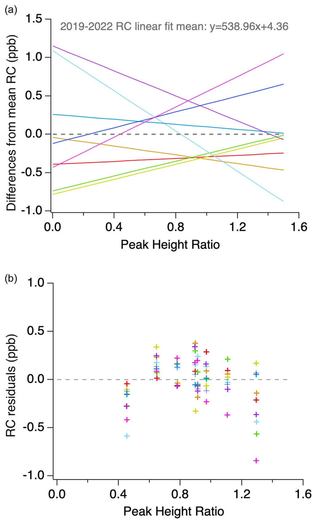
Figure 2 The 2019–2022 H9 standard calibration response curve (RC) results: (a) differences from the mean RC linear fit and (b) residuals of the response curve fits. Different colors are for different calibration episodes.

Since April 2019, a tank air measurement sequence on H9 has consisted of seven tank air injections, each bracketed by reference air injections. The peak heights for the first injections of reference air and tank air can have a small low bias and are not used. The normalized peak heights for the valid tank air injections are converted to H₂ mole fractions using the most recent H9 response function. The average and standard deviation of the retained injection H₂ mole fractions are stored in a database table.

2.2.3 H₂ standards and calibration approach for the flask air analysis system

H₂ in flask air samples is measured in addition to long-lived GHGs (CO₂, CH₄, N₂O, SF₆) and CO by the Measurement of Atmospheric Gases that Influence Climate Change (MAGICC) system in the NOAA GML Boulder laboratory. Until mid-2019, GML operated two nearly identical automated flask air analytical systems: MAGICC-1 (1997–2019) and MAGICC-2 (2003–2014). Since mid-2019, GML has used a new MAGICC-3 system. This new system improved analytical techniques for CO₂, CH₄, N₂O, and CO but continues to use the same GC-HePDD instruments from the older systems.

Two GC-HePDD instruments have been used for hydrogen analysis on the three flask air analysis systems since 2009: H8 (MAGICC-2: 2009–2014; MAGICC-3: August 2019–September 2020) and H11 (MAGICC-1: 2010–July 2019; MAGICC-3: September 2020–present).

On MAGICC-1 and MAGICC-2, the H₂ instrument response was calibrated using a single tertiary standard (measured before and after each sample aliquot), similar to the original one-point calibration approach used on H9.

Out of 17 H₂ tertiary standards used during that time, 3 were used for more than 14 months and 14 displayed H₂ growth over time. Figure 3 shows the calibration histories for H8 and H11 tertiary standards and their deployment dates. For each tertiary standard, assigned mole fractions, drift coefficients, and estimated uncertainties are stored in a database (Table S2). The uncertainty reported in Table S2 is empirically derived and based on the standard calibration history and the standard deviation of the residuals to the best fit (the assignment). The Python code that calculates a secondary- or tertiary-standard assignment uses a 0.5 ppb 1σ H9 reproducibility uncertainty which is added in quadrature to the measurement episode standard deviation to account for longer-term uncertainties not evident in the standard deviation of the n aliquots. We do not formally include an uncertainty for the secondary-standard assignments. The H9 reproducibility term is based on the mean of the standard deviation of residuals to the fit for the calibration histories of secondary standards and target tanks over the period 2008–2022 (see Sect. 2.3.1).

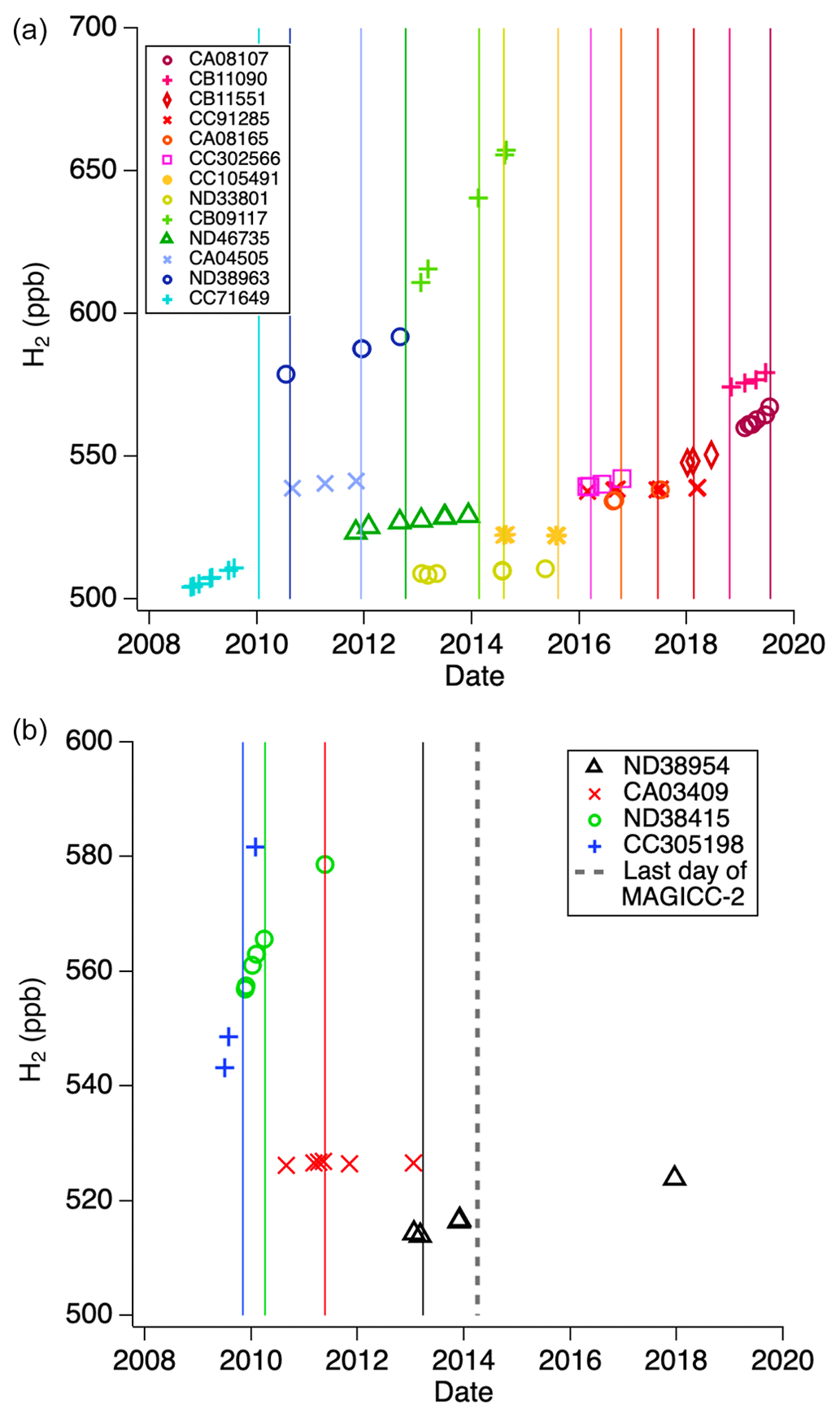
Figure 3 Calibration histories of (a) MAGICC-1/H11 and (b) MAGICC-2/H8 tertiary standards. The colored vertical line indicates when a standard started to be used.

The 17 tertiary standards used successively on the flask analysis systems between 2009 and 2019 introduce time-dependent issues due to the variable rate of H₂ drift in aluminum tanks and the tank calibration histories. Some of the tertiary standards only have pre-deployment calibration results which do not assess drift during use, and other standards have calibration results during their time in use but do not have post-deployment calibrations that may help us evaluate the drift rate for the last couple of weeks or months of use (Table S2, notes in column “N”). Three standards exhibited an increased drift rate towards the end of their life that we did not capture with their infrequent calibrations on H9. This change in drift behavior was observed as increasing biases for measurements of target air tanks and daily test air flasks (see Sect. 3.1.2). We have applied offline mole fraction corrections to the flask air analysis H₂ results to correct for the end-of-use drift increase for these three tertiary standards, and the standards' assignment uncertainty is larger for these time periods (Table S2).

Since August 2019, the MAGICC-3 system has been operated with a GC-HePDD for H₂; new optical analyzers for CO₂, CH₄ (CRDS, Picarro), CO, and N₂O (QC-TILDAS, Aerodyne); and a GC-ECD (electron capture detector) for SF₆. The responses of the instruments are calibrated at the same time using a single set of 11 standards spanning a range of mole fractions for the six trace gases. The MAGICC-3 standards were filled at the Niwot Ridge standard air preparation facility on a few different days between December 2017 and May 2018. Their H₂ mole fractions are regularly measured on H9 against the GML H₂ primary standards.

For the MAGICC-3 instrument response calibration, the 11 standards are analyzed sequentially relative to an uncalibrated reference air tank (filled at Niwot Ridge). Air from each standard is injected six times alternating with the reference air. This entire sequence takes close to 17 h. The first injection of each standard is often biased low by about 2 ppb for H₂ due to timing issues at the start of each standard sequence, and only the remaining five injections are used to obtain the average normalized peak height “signal” for each standard.

For H₂, a subset of 8 of the 11 MAGICC-3 standards are used to determine the GC-HePDD response. The time-dependent H₂ value assignment for each standard was derived from eight or nine calibration events on H9 between June 2018 and December 2022 (Table S3, Figs. S1 and S2). We plan on analyzing the MAGICC-3 standards two to three times a year going forward. The standards' H₂ assignments will be revised as needed. The three cylinders that are not used exhibit complex H₂ growth that is not well captured with periodic calibration episodes and a linear or quadratic fit.

The time between MAGICC-3 instrument response calibration sequences was 2 weeks for the first 3 months of service, and it has been increased to 4–5 weeks as we found the results to be quite stable. A reference air cylinder will last 9 to 12 months on MAGICC-3. When the MAGICC-3 reference air cylinder is changed (pressure close 250 psia), a new instrument response calibration episode is done with the new reference air cylinder before flask air samples are analyzed.

For the asynchronous calibration to stay valid for up to 5 weeks requires the reference gas composition for the six measured gases to be stable between successive calibration episodes. This has been true so far except for one reference air cylinder for which a small time-dependent H₂ correction was applied between two instrument response calibration dates (see Fig. S3 and more details in Sect. S4).

2.3 Calibration scale transfer quality assurance

GML target air tanks are dedicated air mixtures used for measurement quality control over multiple years. Most are high-pressure aluminum cylinders filled at the Niwot Ridge standard preparation facility. The analysis of target air helps us evaluate the robustness of the calibration scale transfer, as well as the consistency of measurements over time and also between different analytical systems. In a perfect program, we should be able to reproduce a measurement result for a target air tank every time. As noted earlier, however, the reality is more complicated as H₂ tends to grow with time in aluminum cylinders. Tracking many aluminum cylinders provides a diverse history of behaviors (stable, or linear vs. nonlinear drift) and aids in the understanding of similar cylinders used for calibration.

2.3.1 Calibration system (H9) target air tanks

Some GML target air cylinders are used exclusively to evaluate the stability and performance of the H9 measurements. Other target air cylinders are analyzed on H9 and in the flask air analysis laboratory on the H8 and H11 instruments to evaluate the scale transfer.

While H₂ has been increasing in most of our target air tanks, 11 H9 target air tanks have shown either stable H₂ or a linear increase of less than 1 ppb yr⁻¹. Figure 4 shows the calibration histories for these tanks as well as the residuals from the best fit for each tank. Table 2 has a list of these target tanks and several others binned by linear drift rate. More details for target tanks are in Table S4. For each bin, the standard deviation of the residuals (differences in the H9 calibration results minus the best fit values) is below 0.5 ppb. The standard deviation of the residuals for all linearly drifting target tanks binned together is 0.4 ppb.

Figure 4 Calibration histories and residuals to best fit for H9 target tanks with a stable H₂ mole fraction or a linear drift less than 1 ppb yr⁻¹. Residuals are in parts per billion.

Table 2 H9 target air tanks with zero or linear growth in H₂.

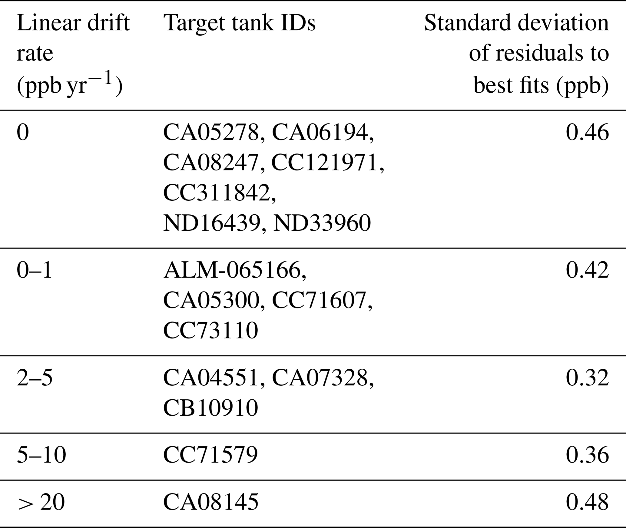
Results for tanks with stable or very slowly drifting H₂ indicate that between 2008 and 2021, the scale transfer on H9 has low uncertainty (< 1 ppb). We have 11 other target tanks for which the best fit to their calibration history is a quadratic function (Fig. S4 and Table S4). The standard deviation of these tanks' residuals binned together is 0.7 ppb. The current set of H9 target air tank results shows that residuals for higher mole fraction (> 650 ppb) tanks have a larger standard deviation (0.5–0.8 ppb, Fig. S4d).

Some tanks that were analyzed soon after fill and over several years show a rapid and large initial growth in H₂ (in the first 0.5–2 years after fill). In this scenario, the residuals to a best linear or quadratic fit of the full calibration history will be larger and will likely not capture the tank time-dependent H₂ assignment as accurately. For a few of the GML standard and target air tanks, we dropped early calibration results that would bias the best fit derivation and assignment during the time of use of the tank.

2.3.2 Comparison of measurements of gas mixtures in cylinders with MPI-BGC

Since 2016, the MPI-BGC GasLab has organized same-tank air measurement (“MENI”) comparisons between WMO GAW partner laboratories as part of the European ICOS (Integrated Carbon Observation System) Flask and Calibration Laboratory quality control work. In this program, three 10 L aluminum cylinders (Luxfer UK) are filled with dry air and maintained by the MPI-BGC and sent to measurement laboratories in a round-robin loop. Two of the three cylinders had the same-air mixture for the 2016–2021 period and showed small growth in their H₂ mole fractions over time. The third cylinder contains an unknown new mixture for each round-robin loop.

Between 2016 and 2021, the MENI cylinders came to GML three times and were analyzed two to four times on the H9 instrument during each round-robin stop. Some results were rejected due to poor instrument performance or the use of an alternate calibration strategy than the one used to transfer the scale. For the blind and the ambient H₂ MENI cylinders the retained NOAA H₂ results agree well with the MPI-BGC measurements (< 1 ppb difference; Fig. S5a, b). For the low-H₂ cylinder, the 2017 and 2018 NOAA measurements are biased low by about 2 ppb, while the 10 March 2021 result is about 2 ppb higher (Fig. S5c). The MENI program provides a valuable ongoing check for the MPI X2009 H₂ calibration scale transfer in GML.

2.3.3 Flask analysis system target air tanks

Figure 5a shows the calibration histories on H9 for target air tanks used in the flask analysis laboratory between 2009 and 2022. H₂ increased in all the target tanks, sometimes rapidly, requiring time-dependent value assignments.

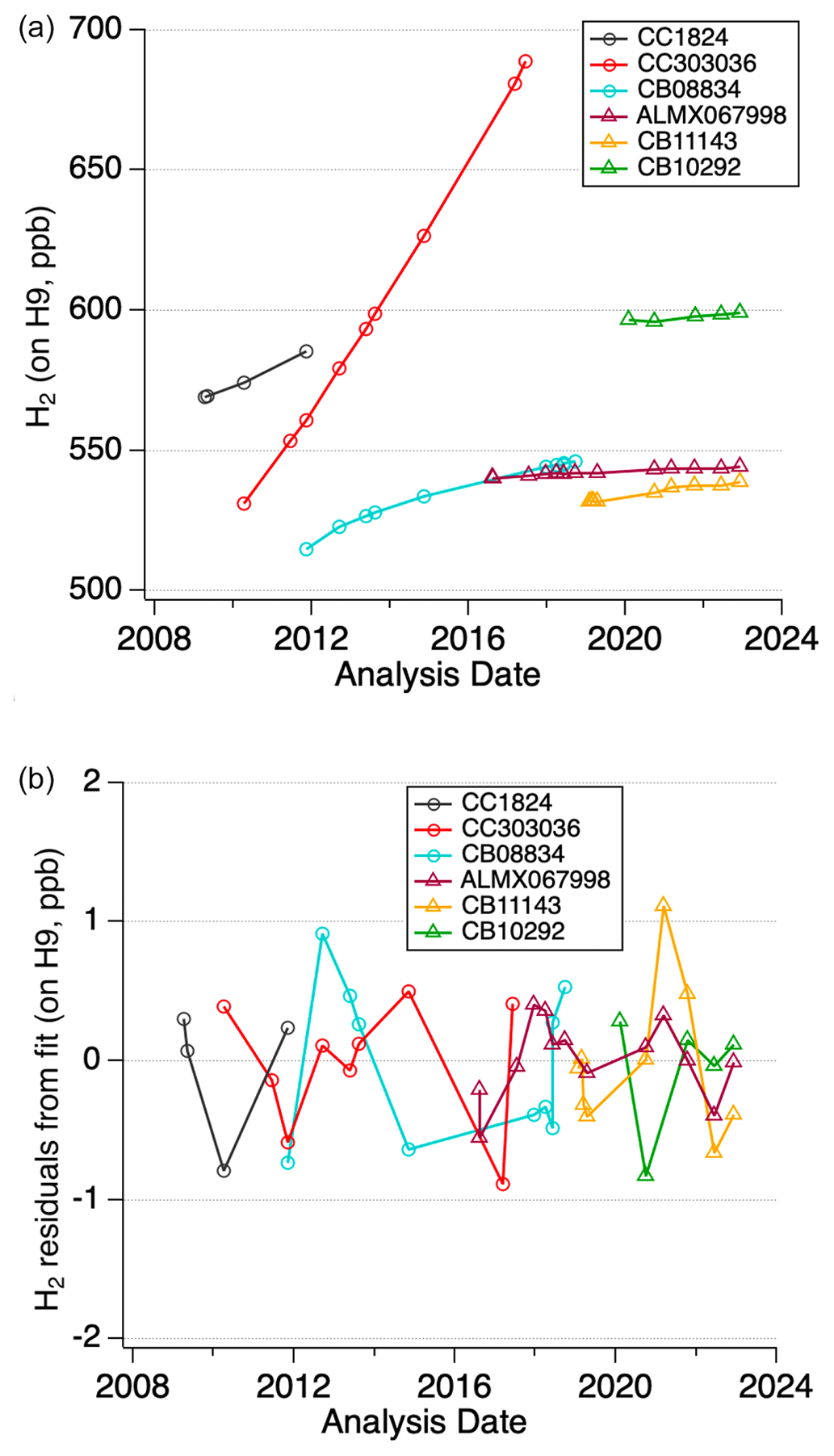
Figure 5 Flask air analysis system target air tank H9 (a) calibration histories and (b) residuals to best linear or quadratic fit.

Three H₂ target air tanks were in service between 2009 and 2019 and have been used to evaluate the GML calibration scale transfer to the MAGICC-1 and MAGICC-2 H₂ measurements (CC1824, CB08834, and CC303036). These tanks, however, exhibited rapid and large drifts and were not measured on H9 on a regular basis, making it more difficult to use them to evaluate potential biases on MAGICC-1 and MAGICC-2 over this time period.

The target air tanks ALMX067998 and CB11143 entered into service in 2016 and 2019, respectively, with more frequent measurements on the calibration system to better define their time-dependent value assignments. A new set of six target air tanks were filled at the Niwot Ridge standard preparation facility in late 2019 for the MAGICC-3 system. They have been analyzed on MAGICC-3 multiple times a year but only one of them has an H₂ mole fraction that remained below 700 ppb: CB10292.

With the caveats that the nonlinear drift in aluminum cylinders may not be well modeled by a simple quadratic polynomial and that many of the early target tanks were under calibrated, the best polynomial fit to the calibration records for all target air tanks gives residuals smaller than 1.2 ppb (Fig. 5b). Details for the target tanks, including the best fit coefficients and the standard deviation of residuals to the fits, are in Table S5.

In Fig. 6, we show the differences between the target tank analysis results on H8 and H11 and their time-dependent H₂ assignments (based on the best fit to their calibration histories on H9 discussed above). The differences are all within 4 ppb; however, there are times when there are persistent biases between the flask analysis system(s) and the calibration system. Uncertainties on the value assignment of the target air tanks, the value assignments, and stability of the standards used to calibrate the flask analysis systems, as well as the noise in the H8 and H11 measurements, all contribute to the observed differences. Similar offsets on both flask analysis systems (for example CC1824 prior to 2012) may point to the main uncertainty contribution being from the value assignment of the target air tank. Different patterns in the offsets between the two flask analysis systems (for example offsets of different signs for CC303036 and CB08834 on H8 and H11 in 2011–2013) suggest the offsets are due to value assignments of the flask analysis system standards. Again, this is often due to limited calibration histories not being able to fully map the nonlinear drift in the standards. It also indicates there are times with systematic differences (mostly < 2ppb) between the MAGICC-1/H11 and MAGICC-2/H8 measurements in the flask records.

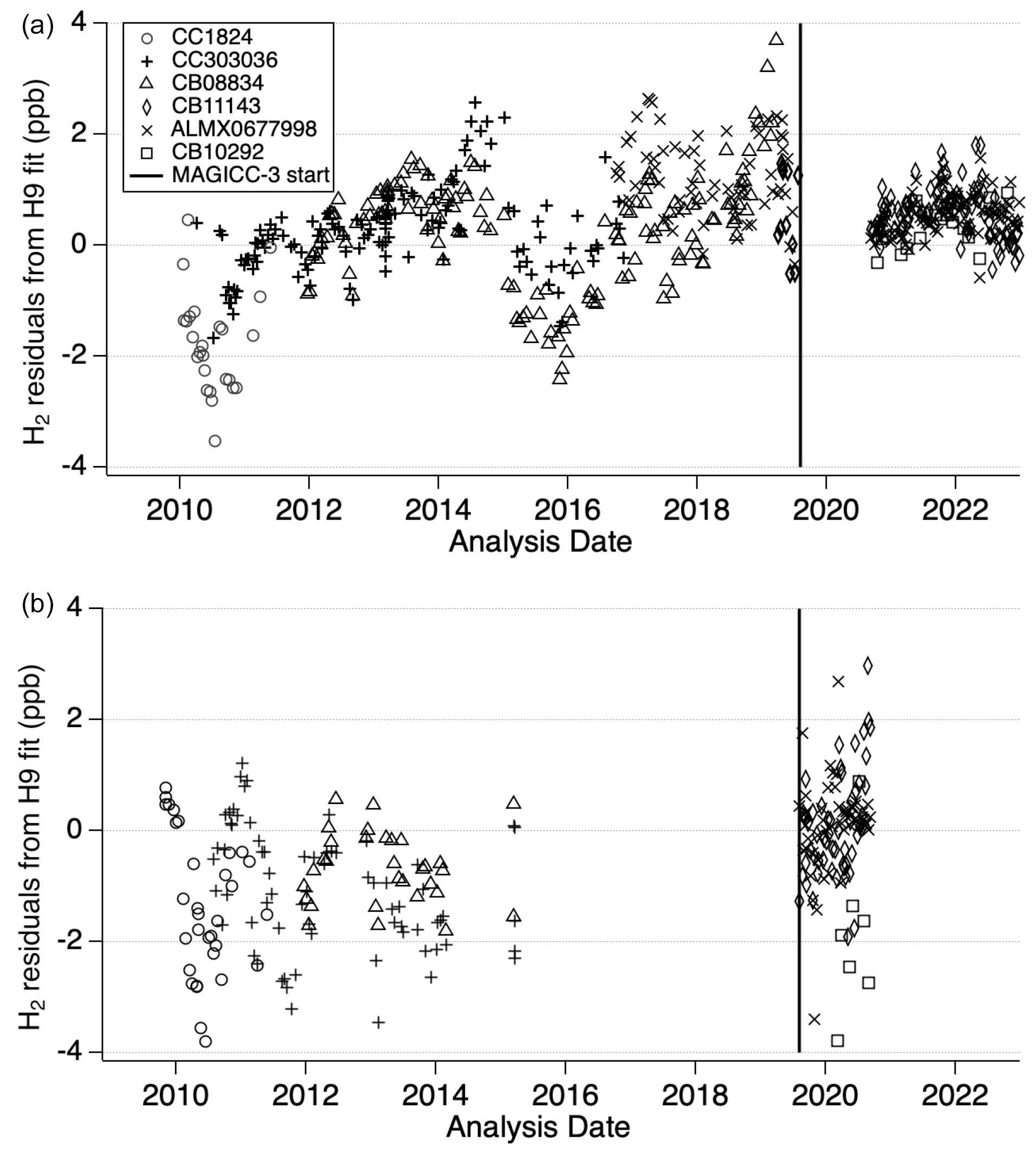
Figure 6 Differences in target air tank H₂ analysis results on (a) H11 and (b) H8 and the time-dependent assignment based on calibration history on H9.

The full transition to the new MAGICC-3 system for flask analyses in August 2019 is indicated by the vertical bar in Fig. 6. As discussed earlier, one improvement in this new system is that H₂ measurements are now calibrated using a multipoint calibration curve from a suite of standards. This makes the measurement results less sensitive to drift or value assignment error in any individual standard since we are fitting multiple standards. We also now appreciate the complex H₂ growth patterns that can occur in aluminum cylinders and so have undertaken regular calibrations to ensure drift is tracked closely. These changes seem to have reduced the bias observed between the flask analysis system and the calibration system, which gives confidence that future measurements will be higher quality.

To help us monitor the H₂ calibration scale propagation performance going forward, a new target air tank in an Essex stainless steel cylinder, SX-1009237, was filled in late 2022 to augment the current target tanks. This target air tank should be stable for H₂ and will be used for periodic comparison between measurement systems. Analysis results on H9 and H11 in December 2022 are 526.75 and 527.15 ppb, respectively, consistent with the residuals for other target air tanks at that time.

3 NOAA flask air H₂ measurements

Close to 6000 flask air samples from the NOAA Cooperative Global Air Sampling Network are analyzed in GML every year. The network sites are chosen carefully to be representative of large-scale air masses and to be able to rely on local support for sampling and shipping logistics. The reprocessing and release of the 2009–2021 H₂ global network flask air measurements on the MPI X2009 scale were made possible because of continued efforts to conduct and improve the H₂ measurements to store all the necessary data and to develop and update the tools for reliable and traceable reprocessing, comparison, and archiving.

3.1 Data quality assurance and quality control

In this section, we first describe the flask sample collection protocol and introduce the data quality control tags used to document sample and measurement data quality issues. GML flask air H₂ measurement data quality is evaluated using results from the daily analysis of test air flask pairs and from the agreement between South Pole Observatory (SPO) flask pairs collected close in time. Finally, we present a preliminary estimation for the uncertainty of flask air H₂ measurements over 2009–2021 that includes empirical uncertainty estimates for the standards' assignments and the short-term noise of the instruments.

3.1.1 Flask air sample collection overview and data quality tagging

Partners in the NOAA Cooperative Global Air Sampling Network collect whole outside air samples in glass flasks in pairs, upwind from any local sources of pollution, people, and animals and away from structures or terrain that would affect the wind flow. Two 2.5 L glass flasks with two glass stopcocks with Teflon O-rings are connected in series in a portable sampling unit (PSU) made of a rugged case, a battery, a pump, an intake line, and a mechanism to control the pressure of the air samples. Most sampling units include a dryer and are semi-automated, with the exception of those used at relatively dry high-latitude locations and a few other locations where a more rugged, manually operated sampling unit is required. At most sites, the operator will carry the equipment outdoors to conduct the sampling. At a few sites, the PSU is indoors and connected to a fixed inlet line drawing air from the outside.

Before flasks are shipped to sampling sites, the glass flasks are filled with synthetic air in the GML flask logistics laboratory. During the sample collection on site, the flasks are first flushed for several minutes and then filled to a pressure of 4 to 5 psi above ambient pressure in about 1 min (see video: https://gml.noaa.gov/education/intheair.html).

Air sample collection and/or measurement issues that are documented or detected and known to affect a sample quality or an analyte measurement result are recorded with data quality control tags in our internal database. For each flask air measurement, internal data quality control tags are translated into a simpler three-column flag indicating if the measurement is retained or rejected for external data users. The GML flask air samples and measurements can also have informational tags and comments, for example if another measurement laboratory analyzed an air sample before it came to GML for analysis (see same-air measurement comparisons in Sect. 3.2).

The global network flasks are filled to a target pressure of 17–20 psia, but the final fill pressure can vary by 3–4 psi, with some of the higher-altitude sites having final pressures on the lower range typically. If an air sample pressure is too low for the H₂ GC instrument on the MAGICC system, the H₂ measurement result is tagged as “rejected” for low sample pressure. If H₂ measurements in paired flasks have a 5 ppb or larger difference, the results for the pair are tagged as rejected. If only one member of the pair had an obvious issue (leak, low flask air pressure), only the H₂ measurement for that member is tagged as rejected. Some issues are detected by the MAGICC performance control system and are tagged automatically. Other issues are tagged manually by scientists as part of regular data quality control checks. Scientists also verify the validity of the automatic tags. Members of the team routinely evaluate if follow-up actions are needed to fix a sample collection or measurement issue or reduce the chance of rejecting future sample results for the same issue.

Some sites can experience brief high-pollution episodes with the H₂ mole fractions in both members of a pair meeting the pair agreement criteria but also being outliers, i.e., outside of the expected long-term variability at the site (Novelli et al., 1999). Gross H₂ outliers are typically “tagged” manually. A statistical filter is also applied to identify outliers before each annual data release (Dlugokencky et al., 1994). For each site, a smoothing curve fit calculation determines the measurement time series mean behavior broken down in a long-term trend, a seasonal cycle, and shorter-term (hours to weeks) variations (Thoning et al., 1989; Tans et al., 1989a). The code is available and a link is provided further down (see “Code and data availability” section). The filter works iteratively to find and tag outlier H₂ measurements when their residuals to the smooth-curve fit are larger than 3 to 4 times the time series residuals' standard deviation.

3.1.2 Test air flask analysis results

Besides the regular analysis of target cylinders, the MAGICC flask analysis system is also tested daily using flasks filled with “test air” (flasks with site code “TST”). We have four rotating high-pressure aluminum cylinders for test air (AL47-104, AL47-108, AL47-113, AL47-145), filled at the Niwot Ridge standard preparation facility. Figure S6 shows their calibration histories on H9 for different fills. H₂ is not stable in the test air cylinders, and for some tank fills, H₂ increased rapidly and grew beyond our calibration range upper limit of 700 ppb.

Every 2 to 3 weeks an even number of TST flasks (14–24) are filled from the same test air cylinder. On typical analysis days, the MAGICC flask air measurement sequence will start with the analysis of air from two TST flasks with the same fill date.

Global network flask air samples are analyzed at NOAA GML only during the daytime to ensure the system operator is overseeing the full analysis cycle and minimizing the time a flask valve is open for the analysis. This is meant to minimize the risk of losing or contaminating the air samples as many of them are subsequently sent to the University of Colorado Boulder Stable Isotopes Laboratory for CO₂ and CH₄ isotope analyses.

Results from the TST flask pairs with the same fill date and analyzed on successive days give an indication of the short-term repeatability of the measurements. Here, the deviations from the mean H₂ in TST flasks with the same fill date are evaluated. For fill dates with a mean H₂ mole fraction less than 700 ppb, we calculate the differences between individual TST flask H₂ and the fill date mean. The standard deviation of the TST flasks H₂ differences from their fill date mean is 1.39 ppb on MAGICC-2/H8 (N = 872), 0.73 ppb on MAGICC-1/H11 (N = 3583), 1.55 ppb on MAGICC-3/H8 (N = 504) and 0.68 ppb on MAGICC-3/H11 (N = 1085), reflecting the higher measurement noise on H8.

Another diagnostic is the comparison of the TST flasks MAGICC H₂ measurement results and their test air cylinders' time-dependent assignments for the dates the TST flasks were filled based on the best fit of the H9 test air tank calibration results. This analysis is limited to the test air with less than 700 ppb H₂ and with tank calibration results on H9 that reasonably capture the increase in H₂: AL47-108 (F), AL47-113 (D, E, G), AL47-145 (F, G), AL47-104 (I). In Fig. S7a–c, we show the H₂ differences between the TST flask results and their test air cylinder assignments. The differences reflect noise in the flask air measurements and uncertainties (and potentially small biases) in the assigned H₂ of the test air tank fill.

Table 3 Summary statistics for H₂ differences between TST flask air measurements and the corresponding test air tank-fill assignments (based on H9 calibration histories).

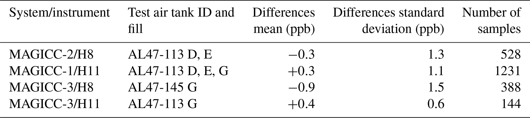
Between 2010 and 2021, the three fills of test air cylinder AL47-113 are in the ambient range and have the most stable H₂ mole fractions. The linear drift rate of the assigned H₂ of the tank fill is 1 ppb yr⁻¹ in fill D, null in fill E, and 0.4 ppb yr⁻¹ in fill G. Table 3 shows the mean and standard deviation of the differences in H₂ between TST flasks and the assigned H₂ in a stable or slowly drifting test air tank fill. The biases for these subsets of TST air data are less than 1 ppb, and the standard deviation is equal to or less than 1.5 ppb and is smaller for the most recent MAGICC-3/H11 configuration, which has a smaller number of data points.

3.1.3 South Pole Observatory: H₂ differences in flask pairs

The South Pole Observatory (site code SPO, sampling location: 89.98° S, 24.80° W; 2810 m above sea level, m a.s.l.) gives scientists access to some of the “cleanest” air on Earth due to its remote location and thus provides an opportunity to use SPO flask data as a quality assurance tool.

Two flask pairs are typically collected weekly and close in time at the four NOAA atmospheric baseline observatories using two collection methods. In method “S”, flasks are filled inside a building by tapping the air continuously pumped for analysis on an in situ GHG measurement system. Method “P” (or “G”) involves using a portable sampling unit with an inlet mast and pump set up outside the building, similarly to other global network sites.

Staff rotation and flask shipping to and from the South Pole Observatory happen during a limited time window during the austral summer. While awaiting shipment, SPO flask air samples are stored in crates in a heated storage building. Every year, one large SPO flask shipment arrives in Boulder in December or January, and another smaller shipment arrives in February or March. A year's worth of flasks is prepared and shipped to SPO during that same time window. Despite the longer storage for SPO flasks before analysis, we have not detected biases in H₂ measurements of those samples when compared with other high-southern-latitude time series. SPO flask air H₂ measurements show close to a 20 ppb seasonal cycle and a ∼ 15 ppb increase in the annual mean levels between 2010 and 2021 (Fig. 7).

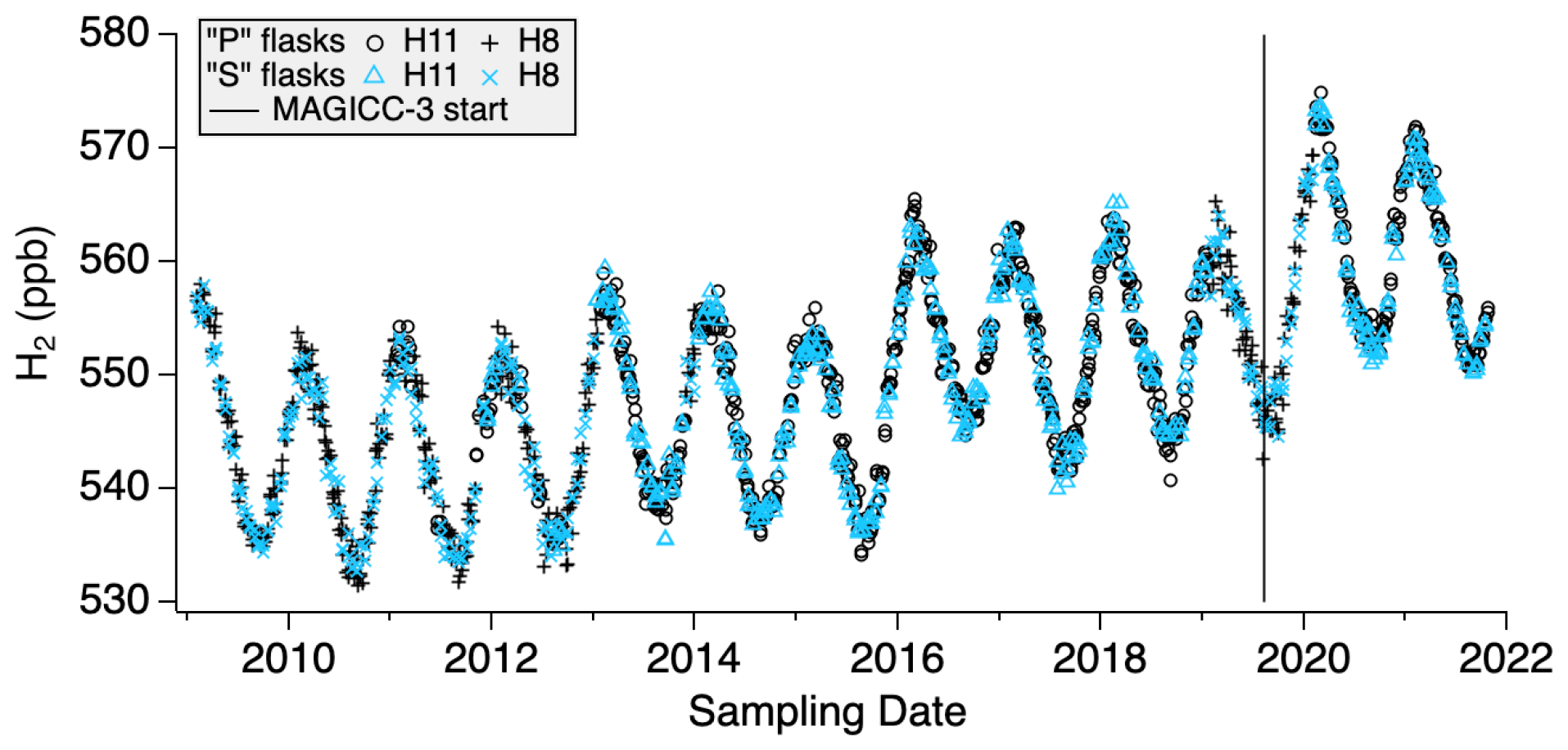
Figure 7 South Pole Observatory flask air H₂ measurements on H11 and H8. Black symbols are used for measurements of P flasks, and blue symbols are used for measurements of S flasks.

There is very little short-term variability in the surface air over Antarctica for long-lived GHGs, CO, and H₂. The differences in the H₂ mole fractions in SPO paired samples therefore mostly reflect the short-term noise in the measurements. In Table S6 we report statistics for H₂ differences for the two flask sampling methods and the four measurement system configurations between 2009 and 2021 with H8 and H11. As observed for the TST flasks, measurements on H11 are less noisy than on H8, especially on the MAGICC-3 system. The average of the absolute differences for H₂ in SPO flask paired samples is less than 2 ppb (σ ≤ 1.3 ppb), and methods S and P H₂ pair averages at SPO agree within 1 ppb on average (σ ≤ 1.7 ppb).

3.1.4 Flask air H₂ uncertainty estimates

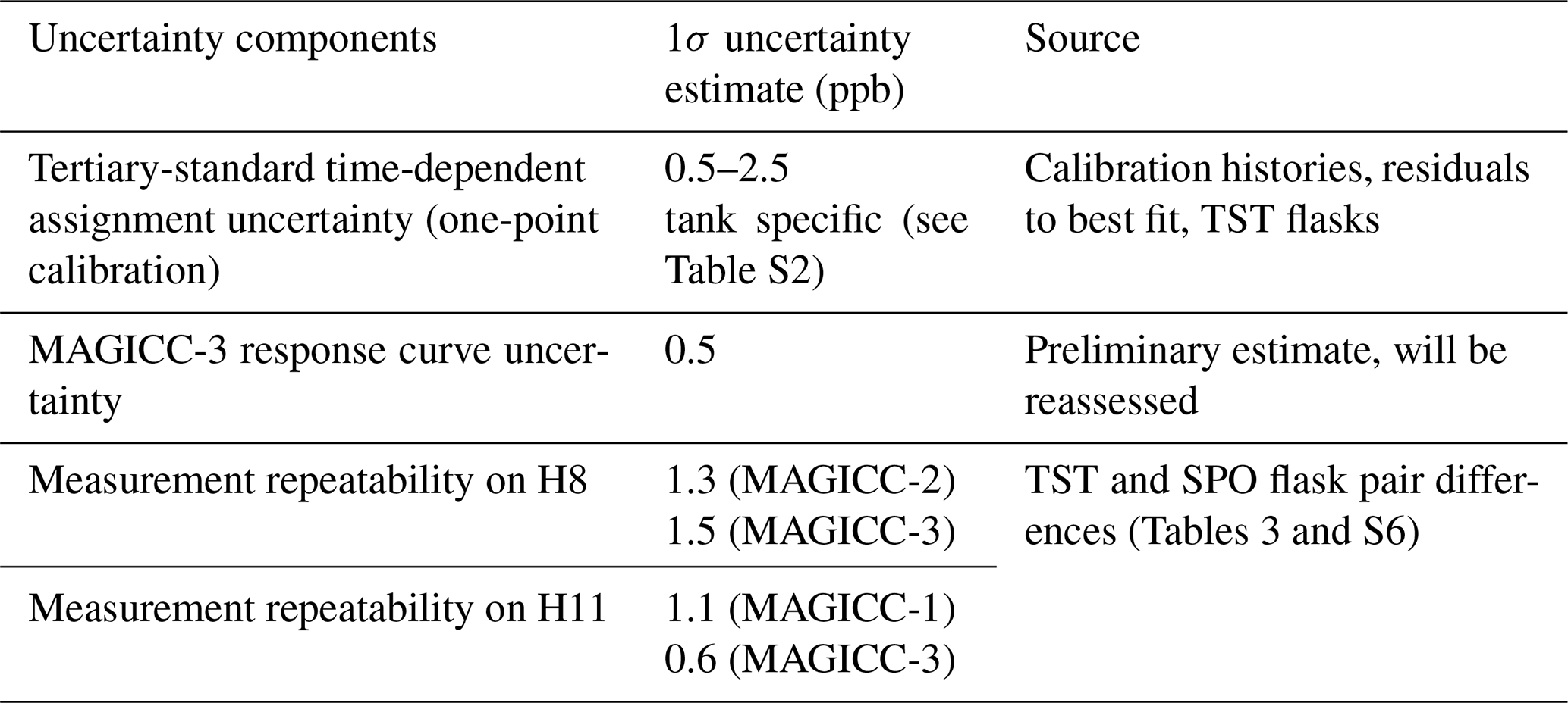
We have derived preliminary empirical uncertainty estimates for flask air H₂ measurements that fall in the 200–700 ppb range. For measurements on MAGICC-1 and MAGICC-2, the total uncertainty estimate comes from the combination of two uncertainties added in quadrature: (1) the uncertainty on the H₂ tertiary-standard time-dependent assignment (Table S2) and (2) the instrument estimated repeatability (Table 4). If an offline assignment correction is applied to take into account changes in a standard drift rate toward the end of its use, the standard assignment uncertainty is increased. The H8 and H11 instrument repeatability estimates are listed in Table 4. For now, we assume a 0.5 ppb uncertainty on the MAGICC-3 instrument response calibrated with multiple standards. Ongoing work will allow us to refine this last uncertainty component estimate at a later date. Typical 1σ uncertainties for GML flask air H₂ measurements are 1.2 to 1.9 ppb on MAGICC-1, 1.4 to 2.8 ppb on MAGICC-2, 1.6 ppb on MAGICC-3/H8, and 0.8 ppb on MAGICC-3/H11.

Table 4 Flask air H₂ measurement uncertainty components.

3.2 Comparison with other GAW laboratory H₂ measurements

A small number of laboratories operate well-calibrated long-term measurements of important atmospheric trace gases. The WMO GAW coordinates regular technical and scientific discussions with experts from these laboratories. Another important outcome of the WMO GAW collaborations consists of routine comparisons to assess the data compatibility for measurements from different laboratories and programs (Francey et al., 1999; Masarie et al., 2001; Jordan and Steinberg, 2011; Worthy et al., 2023). The WMO GAW network compatibility goal for measurements of H₂ in well-mixed background air is 2 ppb (see Table 1 in WMO, 2020). This means that for H₂, measurement records should not have persistent biases larger than 2 ppb to be used in combination with other qualifying measurements in global budget, trend, and large-scale gradient analyses.

GML participates in several WMO GAW measurement comparison efforts. Same-flask air measurement comparisons consist of one member of a NOAA flask pair collected at a site being analyzed by a partner laboratory before being analyzed by GML. Colocated flask air measurement comparisons involve two or more measurement programs having samples collected at the same location and close in time. Historically, these and other “intercomparison” projects have been abbreviated ICPs, which we use in the text below. Here the GML flask air H₂ measurement compatibility is assessed with results from ongoing ICPs.

GML conducts same-flask air measurement comparisons at the Kennaook/Cape Grim Observatory (CGO; 40.68° S, 144.69° W; 164 m a.s.l.) with CSIRO, Australia, and at the Ochsenkopf mountain top tower (OXK; 50.03° N, 11.81° E; 1085 m a.s.l.) with MPI-BGC, Germany. Sampling at OXK was temporarily suspended between June 2019 and April 2021. The Alert/Dr. Neil Trivett Observatory (ALT; 82.45° N, 62.51° W; 190 m a.s.l.) has facilitated the largest multi-laboratory flask air comparison experiment in the WMO GAW program (Worthy et al., 2023). NOAA has colocated flask air samples from ALT with CSIRO and the MPI-BGC. The CSIRO and MPI-BGC H₂ measurements are also traceable to the MPI X2009 calibration scale.

Table 5 Annual mean of H₂ measurement differences (in ppb) for air samples from the Kennaook/Cape Grim Observatory (CGO), Ochsenkopf (OXK), and Alert (ALT). Non-background air sample measurement results are included. Colocated (not same-air) samples at ALT are matched within a ±60 min window.​​​​​​​

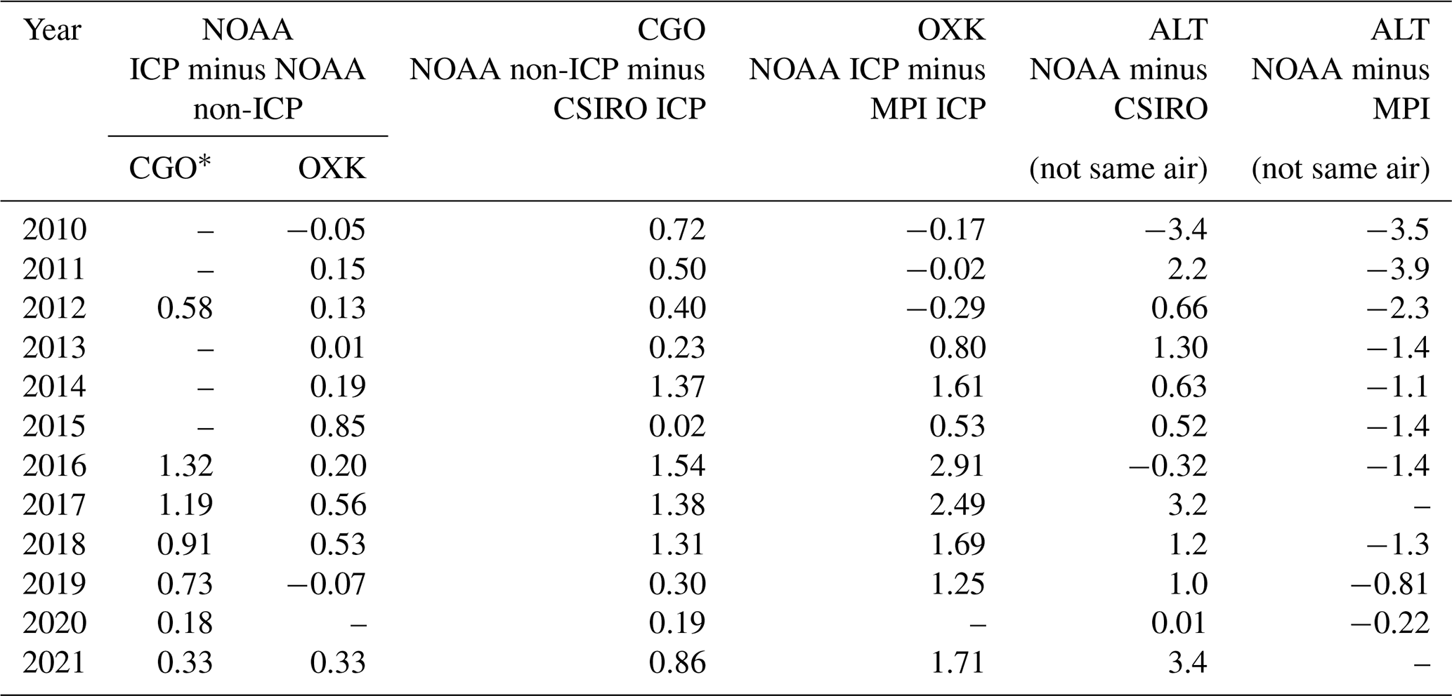
^∗ Most NOAA ICP flasks from CGO had a small contamination for CO and H₂ prior to 2019. If the NOAA ICP flask H₂ results are > 2 ppb larger than the NOAA non-ICP flask H₂ in the pair, the ICP flask H₂ has been rejected. Only years with at least 10 valid H₂ pairs are included.

In Table 5, we summarize the annual mean of the differences for H₂ measurements from different laboratory and flask combinations (same flask, same flask pair, or colocated flasks) for CGO, OXK, and ALT between 2010 and 2021. All measurements included in the comparisons are retained, meaning they have passed quality control checks.

Columns 2 and 3 show the annual means of the NOAA H₂ measurement differences between the ICP flask and its pair mate at CGO and OXK. For CGO flask air samples collected before 2019, we find that the NOAA analysis for the NOAA ICP flask first measured at CSIRO often shows higher H₂ than in the non-ICP flask air sample. We suspect several of these ICP flasks had a small but detectable contamination for H₂. We have applied a rejection tag to NOAA analysis results for CGO ICP flasks with an H₂ mole fraction of 2 ppb or more above H₂ in the non-ICP pair mate. This affected 165 ICP samples between 2009 and 2018 or 37 % of all CGO ICP flasks collected between August 2009 and the end of 2021. For OXK, the NOAA analysis result for the ICP flask first measured at MPI-BGC often shows slightly higher H₂ than for the non-ICP flask (Table 5, third column), and the annual mean bias is less than 1 ppb for all years.

The last four columns in Table 5 show interlaboratory H₂ measurement comparisons for CGO, OXK, and ALT flask air samples. The annual mean differences are consistently less than 1.6 ppb for CGO and less than 2 ppb for OXK for 9 out of 11 years (Fig. 8). For colocated air samples at ALT we compare the mean of flask results for each laboratory and limit the comparison for samples collected within 60 min of each other. The ALT annual mean differences vary from year to year and are less than ±2 ppb for 8 years out of 12 for the NOAA vs. CSIRO comparison and for 7 years out of 10 for the NOAA vs. MPI-BGC comparison. These ongoing ICPs are monitored regularly to continually assess the NOAA H₂ data compatibility with data from GAW partners.

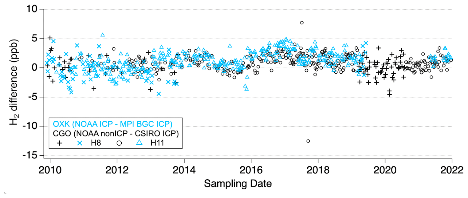
Figure 8 Interlaboratory same-air H₂ measurement difference for OXK ICP (NOAA minus MPI-BGC) and CGO (NOAA non-ICP minus CSIRO ICP).​​​​​​​

4 NOAA atmospheric H₂ time series

Previous measurement studies have described the H₂ global distribution for different time periods (Khalil and Rasmussen, 1990; Novelli et al., 1999; Langenfelds et al., 2002; Price et al., 2007; Yver et al., 2011). Some of the spatiotemporal features in the more recent NOAA H₂ measurement records are described in this section.

4.1 H₂ at the NOAA Cooperative Global Air Sampling Network sites

There are 51 sites considered active or recently terminated in the Cooperative Global Air Sampling Network (see map in Fig. S8 and site information in Table S7). The H₂ measurement time series for these sites are shown in Fig. S9. Note that a few sites that have been discontinued are not shown in this figure. A curve fit is run for each site time series based on Thoning et al. (1989). First the code optimizes parameters for a function made of a four-term harmonic and a cubic polynomial. The resulting residuals (measurements minus function) are then smoothed with a low-pass filter with a 667 d cutoff and are added to the polynomial part of the function to produce the “trend curve” (shown as the dark blue line in Fig. S9). The residuals are also smoothed with a low-pass filter with an 80 d cutoff and are added to the function to produce a “smooth curve” at each site.

The data quality control work on our long-term measurement time series includes a data selection step with a statistical filter (also mentioned in Sect. 3.1.1). Samples with H₂ beyond 3 to 4 standard deviations (depending on the site) of the time series smoothed curve at a site are flagged as outliers, i.e., not representative of background air conditions, and are shown as crosses in Fig. S9.

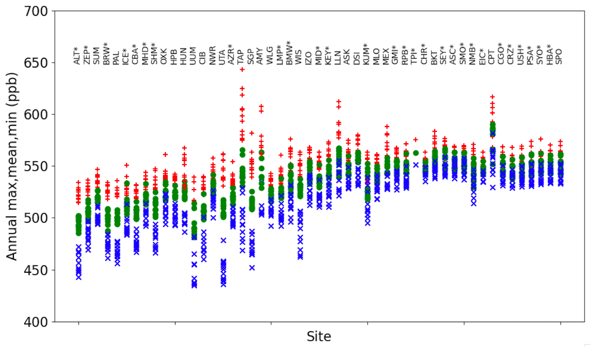
Figure 9 Annual maximum (red), mean (green), and minimum (blue) H₂ from the smooth-curve fit of the 2010–2021 measurement time series for each surface site in the global sampling network. Each site is referred to with a three letter code (see details in Table S7). The sampling sites are shown along the x axis with decreasing latitudes. An asterisk near the site code indicates if the site data are used for the marine boundary layer air zonal and global mean H₂ data reduction.

The annual mean, maximum, and minimum H₂ values of the smooth curve for the 51 network sites are plotted in Fig. 9 (in order of decreasing latitude along the x axis) for years with retained measurements up to 2021. Sampling at the TPI site, on Taiping Island, Taiwan, started in May 2019, which explains the two (full sampling year) data points for the site. Sampling at a few network sites was impacted by the COVID-19 pandemic resulting in data gaps or delayed return shipping of samples. We recommend data users become familiar with individual sampling site measurement records to best aggregate and interpret signals.

The interhemispheric gradient of H₂, with higher levels in the SH, is apparent in the annual mean distribution across sites (Fig. 9, green circles). The majority of sites in the SH (Bukit Kototabang, Indonesia (BKT), to SPO on the right side of Fig. 9) shows smaller seasonal-cycle amplitudes (< 23 ppb) than NH sites; however, several sites have interannual variations in their H₂ seasonal-cycle amplitudes (Fig. S9). Sites with the lowest H₂ seasonal minima (Fig. 9, blue X symbols) likely are the most influenced by soil uptake. A few sites (e.g., TAP, AMY (Republic of Korea), LLN (Taiwan), CPT (South Africa)) show higher smooth-curve annual maxima (Fig. 9, red crosses), likely reflecting upwind local or regional emissions.

4.2 H₂ at NOAA Baseline Atmospheric Observatories

NOAA GML operates four staffed atmospheric baseline observatories (https://gml.noaa.gov/obop/, last access: 23 July 2024). The South Pole Observatory in Antarctica and the Mauna Loa (MLO, Hawaii) observatories were built in connection to the 1957–1958 International Geophysical Year, a global effort bringing together 67 nations to study the Earth and in connection with the first launches of artificial satellites in Earth's orbit by the USA and the former Soviet Union. The South Pole Observatory in Antarctica was established with support from the US National Science Foundation and NOAA. The other two observatories near Utqiaġvik, formerly Barrow (BRW), and Samoa (SMO) were established in 1973 and 1974, respectively.

All four NOAA atmospheric baseline observatories have an upwind clean-air sector with no local sources of pollution. Every week, scientists on location collect discrete air samples preferentially when the near-surface wind comes from the clean-air sector (see earlier Sect. 3.1.3). Figure 10 shows the reprocessed H₂ time series for the observatories between 2009 and 2021. Valid “S” and “P” method flask air H₂ measurements are retained for the South Pole Observatory only. The “S” method flasks show contaminated H₂ at Samoa and show seasonal contamination at Utqiaġvik (Barrow) until August 2021 when sampling started at a new tower with new sampling lines. The Mauna Loa H₂ in “S” method flasks will be further evaluated and may be retained in future releases.

Figure 10 H₂ time series at the NOAA Atmospheric Baseline Observatories.

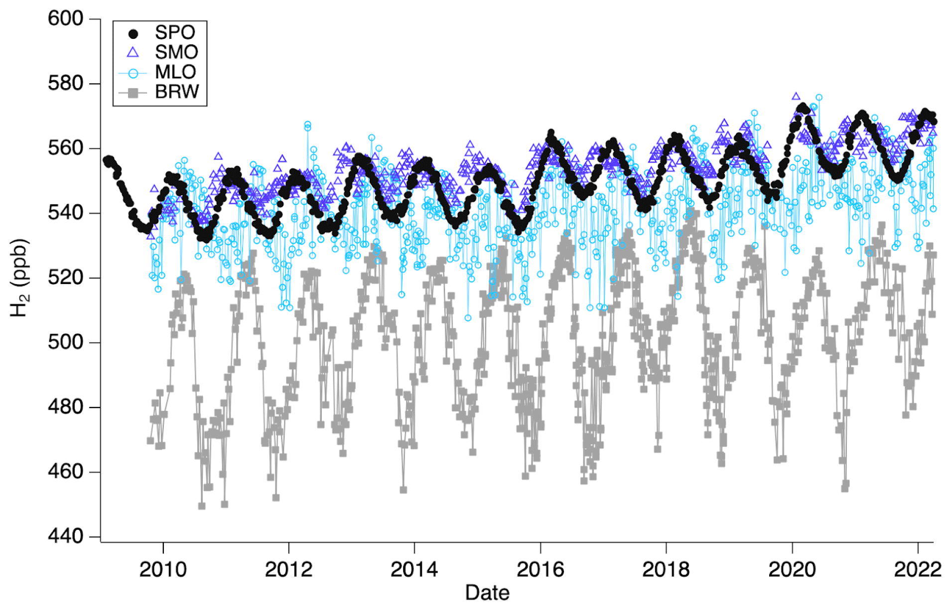
The Samoa and South Pole H₂ smooth curves show similar maximum levels between 550 and 570 ppb and slightly higher minima at Samoa compared to the South Pole. The seasonal maximum occurs about 3 months earlier at Samoa than at the South Pole. The interannual variability is similar at both sites and is dominated by three step increases in 2012/2013, 2016, and 2020.

The Mauna Loa H₂ time series shows more short-term variability than for Samoa and the South Pole. The seasonal-cycle amplitude of the Mauna Loa H₂ smooth curve is about 40 ppb with maximum levels in April–May and minimum levels in December–January. The seasonal maximum ranges from 550 to 580 ppb, and the seasonal minimum ranges from 505 to 520 ppb. The measurements indicate that annual mean H₂ levels at Mauna Loa after 2016 were higher than in previous years.

Of the four observatories, the Barrow H₂ time series shows the lowest levels and the strongest seasonal cycle, about 60 ppb on average. The smooth-curve seasonal maximum ranges from 520 to 540 ppb in April–May, and the seasonal minimum in September–November ranges from 450 to 490 ppb.

Despite having larger emissions in the NH, the H₂ interhemispheric gradient shows lower levels in the extratropical NH. This is related to the larger land masses in the NH and the soil sink being the dominant removal process for H₂. Warwick et al. (2022) report model-based estimates for the H₂ lifetime of 8.3 years for the OH sink (from the authors' base model configuration) and of 2.5 years for the soil uptake (average of existing literature studies). In their flux inversion, Yver et al. (2011) estimated that the NH high latitudes and the tropics represent 40 % and 55 % of the global soil sink, respectively. The soil sink and OH sink in extratropical northern latitudes both peak in summertime (Price et al., 2007), leading to the observed stronger H₂ minima.

It is important to look at data from multiple sites to study and detect interannual and potentially long-term large-scale changes in atmospheric H₂ levels. In the next section, we present background air zonal mean H₂ time series based on samples collected at marine boundary layer sites.

4.3 H₂ marine boundary layer global and zonal means

To extract large-scale signals from the global air sampling network, we use the NOAA GML marine boundary layer (MBL) zonal data product (Tans et al., 1989b; Dlugokencky et al., 1994). Time series from remote MBL sites are smoothed and interpolated to produce a latitude vs. time surface of the H₂ mean MBL mole fraction (Fig. 11). For H₂, the number of sites included in the zonal mean calculations ranges from 29–42 sites until July 2017 when sampling from the Pacific Ocean shipboard (POC) was stopped, after which 24–27 sites were included in the calculation (see also in Fig. 9 MBL site codes with an *). Because the NOAA Cooperative Global Air Sampling Network is sparse in the tropics and in the SH midlatitudes, the MBL product likely does not equally detect and reflect interannual variability in fluxes in these under-sampled regions, for example biomass burning emissions in Africa and South America.

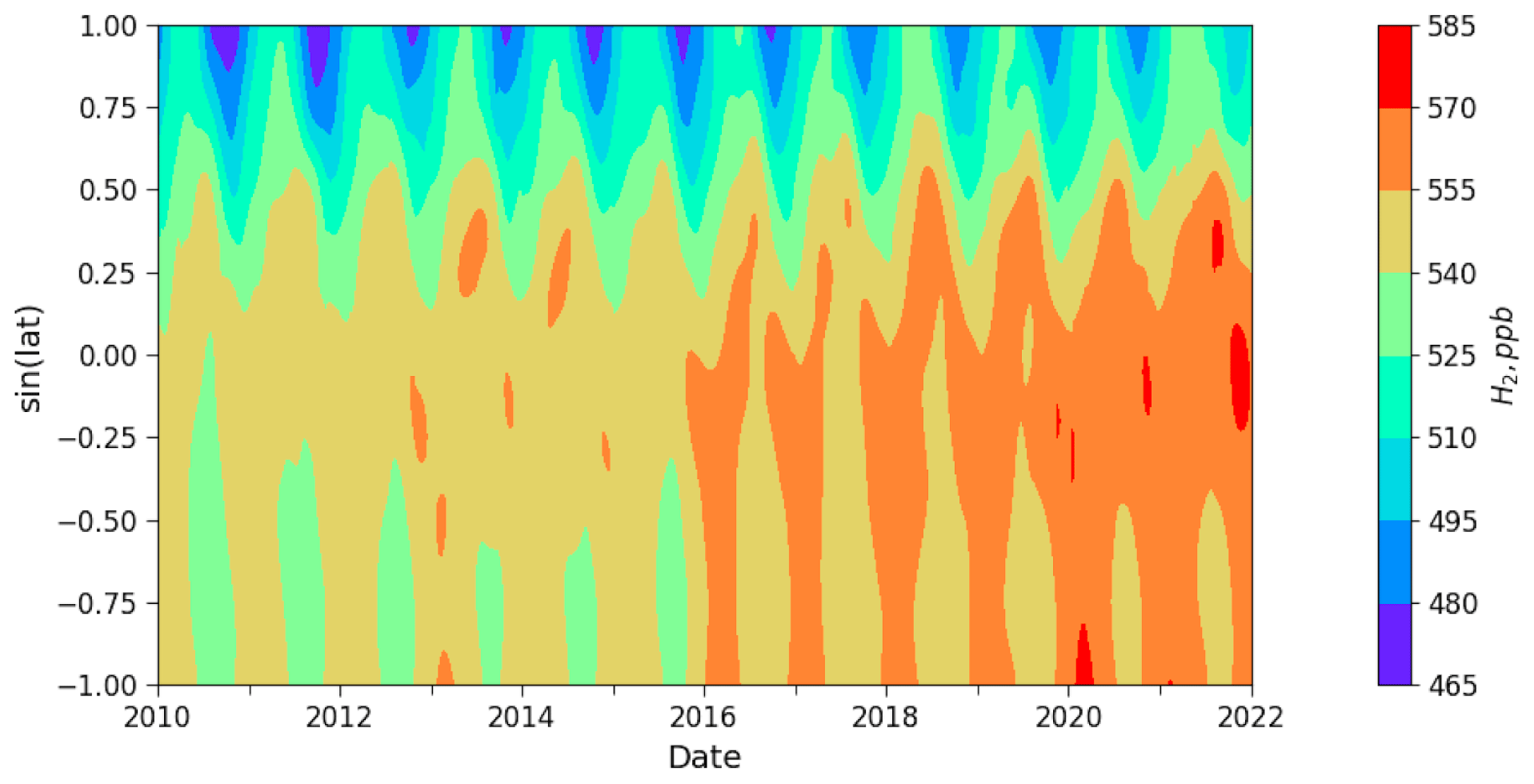
Figure 11 The 2010–2021 marine boundary layer H₂ meridional gradient. The y axis is the sine of latitude.

To further isolate changes in background H₂ at different latitudes, we first calculate MBL global and zonal means (shown in Fig. S10) and then derive anomalies by removing the 2010–2021 average year from the global and zonal mean time series. Figure 12 shows the MBL anomaly for H₂ (black lines) and CO (dashed blue lines) for the global mean and five zonal band means (​​​​​​​NH and SH polar (53–90°), NH and SH temperate (17.5–53°), and tropics (17.5° S to 17.5° N)). The NOAA GML CO measurements are for the same-air samples as the H₂ measurements (Pétron et al., 2023b). Here, we derive the global and zonal means for CO using the 2009–2022 MBL CO measurements, and the anomalies are based on the 2010–2021 smooth-curve zonal mean results to be consistent with the H₂ data analysis.

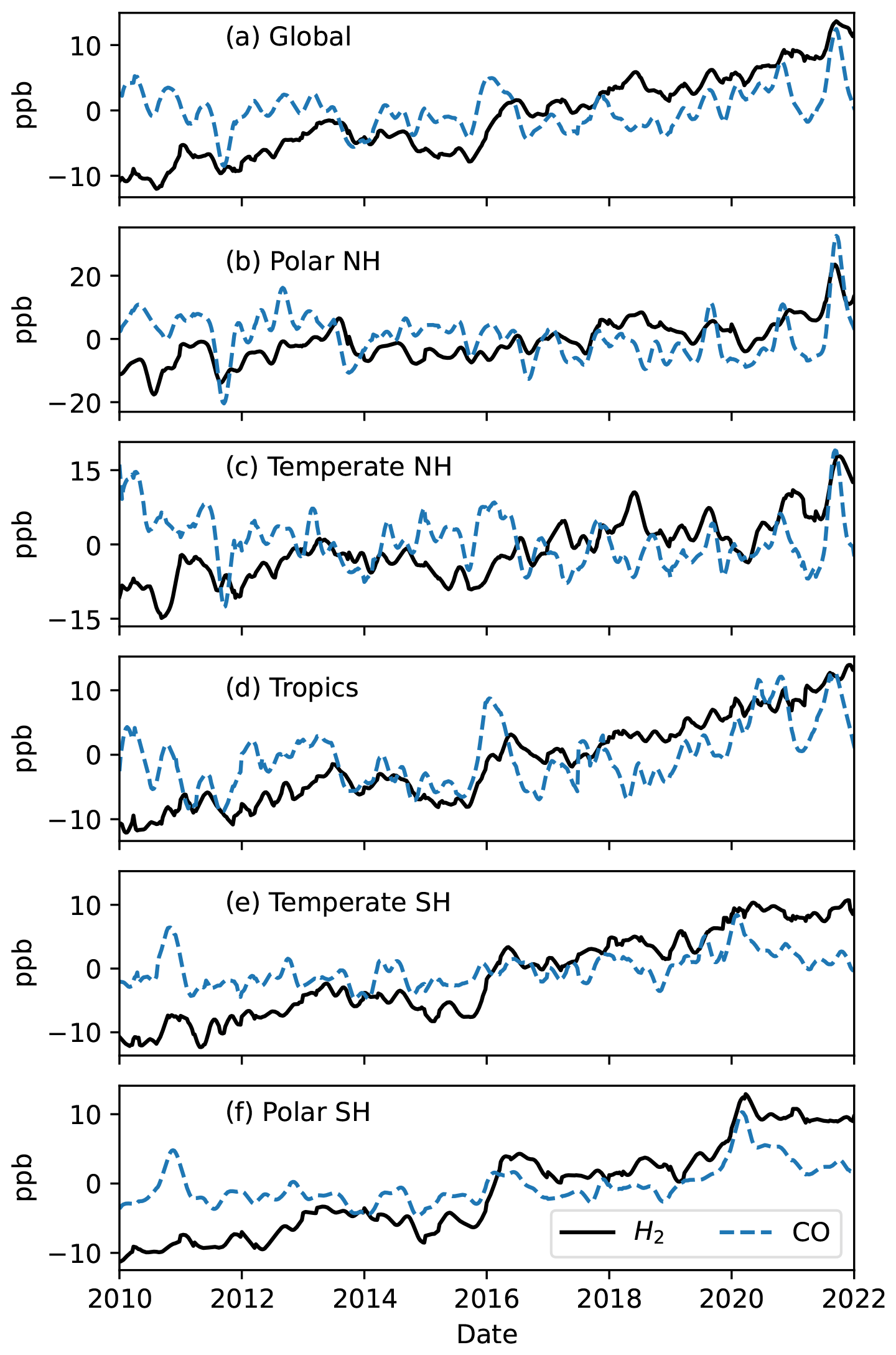
Figure 12 The 2010–2021 marine boundary layer global mean and zonal mean H₂ anomaly (black line) and CO anomaly (dashed blue line) time series.

CO is emitted during incomplete combustion and is a useful marker of biomass burning emissions. CO has a shorter atmospheric lifetime than H₂, which results in shorter-lived CO anomalies from pulse emissions. The data reduction for the anomaly analysis is slightly different from Langenfelds et al.'s (2002) investigation of CO₂, CH₄, H₂, and CO interannual variability in the CSIRO network 1992–1999 time records. The CSIRO authors employed the same (Thoning et al., 1989) data-smoothing technique as we do but used the derivative of the trend curve to analyze correlations in interannual growth rate variations between species. The anomaly approach chosen here allows us to more closely retain the timing of abrupt changes in the measurement records.

Over 2010–2021, background air H₂ has increased at all latitudes (Fig. 12). The global mean MBL H₂ shows a non-uniform increase over this time with a noticeable 10 ppb step increase in 2016. The global mean MBL H₂ was 20.2 ± 0.2 ppb higher in 2021 compared to 2010 (Fig. 12a).

The meridional gradient and zonal band mean plots (Figs. 11 and 12) highlight the evolution of background air H₂ at different latitudes. Anomalies in the smooth curves are useful to point to time periods when several successive air samples at a site show similar deviations from the average seasonal cycle and multiyear trend.

The 2016 H₂ step increase is detected in the tropics and SH. In the tropics it coincides with a strong positive CO anomaly that started in November 2015, reached a peak amplitude of 15 ppb in mid-January 2016, and ended in May 2016. The 2015/2016 H₂ anomaly is first detected at Bukit Kototabang, Indonesia (BKT), and later at Ascension Island (ASC), Kennaook/Cape Grim Observatory (CGO), and Crozet Island (CRZ). Some BKT air samples impacted by biomass burning emissions show enhancements of hundreds of parts per billion in CO and H₂ (Fig. S11). The 2015 fire season in Indonesia was among the most intense on record as shown by remote sensing products of fire counts, CO, and aerosols. Field et al. (2016) found that burning activities to clear peatland for farming likely contributed to larger emissions than expected from dry conditions alone in 2015.

There is another step increase in the polar SH zonal band in early 2020, also coinciding with a pulse anomaly in CO (Fig. 12f) likely related to large wildfires in Australia in late 2019–early 2020. The Kennaook/Cape Grim Observatory (CGO) and Crozet Island (CRZ) smoothed curves show a large jump between the late 2019 minimum and early 2020 maximum when the CGO CO measurement seasonal minimum is also 10–12 ppb higher than in other years (Fig. S11). Van der Velde et al. (2021) estimate that the 2019–2020 fires in Australia emitted 80 % more CO₂ than “normal” Australian annual fire and fossil fuel emissions combined.

In the NH extratropic bands, positive anomalies of H₂ in 2021 coincide with CO pulse anomalies (Fig. 12b–c). For the polar (temperate) NH zonal band, the CO anomaly lasts from mid-July (June) to December 2021 with a peak in September and an anomaly maximum amplitude of 37 ppb (19 ppb). Record high emissions of CO₂ and CO from boreal forest fires in Eurasia and North America in 2021 have been reported by Zheng et al. (2023).

Previously, Simmonds et al. (2005) and Grant et al. (2010) have reported on the observed variability in the Mace Head continuous H₂ measurement record and linked interannual variability in the baseline annual mean H₂ to larger fire emission events. More recently, Derwent et al. (2023) shared an updated analysis of the February 1994–September 2022 Mace Head in situ H₂ measurements. The in situ record shows higher monthly mean baseline H₂ levels in recent years, and the authors report an increase in monthly mean anomalies after December 2015 (slope of 2.4 ± 0.5 ppb yr⁻¹). They postulate that a “missing” source of increasing intensity after 2010 may be behind the observed sustained increased H₂, which is markedly different from the 1998–1999 anomalies attributed to biomass burning. Derwent et al. (2023) explore potential candidates for the missing sources. However, in the absence of strong and quantitative direct evidence at this time, additional studies are needed to interpret the observed H₂ variability.

5 Conclusions

In this paper, we have described how NOAA GML has adopted the MPI X2009 H₂ calibration scale. The work was confined to measurements on GC-HePDD instruments. The GML H₂ primary standards in electropolished stainless steel cylinders have been calibrated once by the MPI-BGC CCL in fall 2020. We have used the CCL assignments to propagate the scale to secondary and tertiary standards. H₂ increases in most air standards stored in aluminum cylinders. A curve fit was applied to each standard calibration history to determine a time-dependent H₂ assignment on MPI X2009. The secondary- and tertiary-standard H₂ assignments were then used to reprocess results for NOAA flask air H₂ measurements on MPI X2009. The reprocessed NOAA Cooperative Global Air Sampling Network flask H₂ measurements for 2009–2021 are publicly available (Pétron et al., 2023a). For the period 2010–2021, same-air measurements with GAW partner laboratories have annual mean differences of less than 2 ppb for the Kennaook/Cape Grim Observatory comparison with CSIRO and less than 3 ppb for the Ochsenkopf comparison with MPI-BGC. Over 2010–2021, background air H₂ has increased at all latitudes. However, site time series and marine boundary layer H₂ zonal means show significant interannual variability. We find that some of the strongest H₂ zonal mean anomalies coincide with CO anomalies and therefore were likely partly driven by large biomass burning events in Indonesia (2015), Australia (2019/2020), and boreal latitudes (2012 and 2021) (Field et al., 2016; Petetin et al., 2018; Zheng et al., 2023). A full analysis of the NOAA Cooperative Global Air Sampling Network H₂ measurement records is beyond the scope of this paper. An early observation and global model comparison is in Paulot et al. (2024). The NOAA H₂ dataset complements WMO GAW partner laboratory H₂ measurements, and it will be updated and extended routinely moving forward.