the Creative Commons Attribution 4.0 License.
the Creative Commons Attribution 4.0 License.
 | 26 Aug 2024
High-altitude balloon-launched uncrewed aircraft system measurements of atmospheric turbulence and qualitative comparison with infrasound microphone response
Anisa N. Haghighi
Ryan D. Nolin
Gary D. Pundsack
Nick Craine
Aliaksei Stratsilatau
This study investigates the use of a balloon-launched uncrewed aircraft system (UAS) for the measurement of turbulence in the troposphere and lower stratosphere. The UAS was a glider which could conduct an automated descent following a designated flight trajectory and was equipped with in situ sensors for measuring thermodynamic and kinematic atmospheric properties. In addition, this aircraft was equipped with an infrasonic microphone to assess its suitability for the remote detection of clear-air turbulence. The capabilities of the UAS and sensing systems were tested during three flights conducted in New Mexico, USA, in 2021. It was found that the profiles of temperature, humidity, and horizontal winds measured during descent were in broad agreement with those made by radiosonde data published by the US National Weather Service, separated by up to 380 km spatially and by 3 to 5 h temporally. Winds measured during controlled flight descent were consistent with the winds measured by global-positioning-system-derived velocity during balloon ascent. During controlled descent with this particular payload, a nominal vertical resolution on the order of 1 m was achieved for temperature, relative humidity, and pressure with a nominal vertical resolution of the wind velocity vector on the order of 0.1 m; the aircraft had a glide slope angle from 1 to 4° during this time. Analysis approaches were developed that provided turbulent kinetic energy and dissipation rate, but it was found that the corresponding Richardson number was sensitive to the methodology used to determine the vertical gradients from a single flight. The low-frequency content of the infrasonic microphone signal was observed to qualitatively align with long-wavelength wind velocity fluctuations detected at high altitude. Moreover, the microphone measured more broadband frequency content when the aircraft approached turbulence produced by the boundary layer.
- Article
(14491 KB) - Full-text XML
- BibTeX
- EndNote


By enhancing the exchange of mass, momentum, and energy, the formation and evolution of atmospheric turbulence provides a significant contribution to weather and climate. As atmospheric turbulence is expected to increase in frequency and intensity in response to climate change (e.g., Williams and Joshi, 2013), a better understanding of its role in atmospheric dynamics is needed. The presence of atmospheric turbulence, particularly clear-air turbulence, also poses an aviation hazard that is challenging to predict and detect. This latter point is particularly true for high-altitude autonomous flight, a regime which is being increasingly pursued in the form of high-altitude pseudo-satellite aircraft intended to provide communication and remote observation capabilities at relatively low cost (Gonzalo et al., 2018; D'Oliveira et al., 2016; Hasan et al., 2022). By the nature of the low-density conditions under which these aircraft are designed to operate, they tend to be lightweight with narrow performance envelopes for which controlled flight can be maintained, making them susceptible to atmospheric disturbances. Hence, there is motivation to improve our ability to measure and predict stratospheric and upper-tropospheric turbulence, which can occur due to shear instabilities or gravity wave breaking despite the higher static stability at these altitudes. Turbulence in the upper troposphere may also be introduced through mesoscale convective systems (Liu et al., 2014), mountain waves (Cunningham and Keyser, 2015), and wind shear (e.g., as introduced by the jet stream).
Although the turbulence intensity is commonly quantified through the turbulent kinetic energy per unit mass,
atmospheric turbulence is often also characterized through the related turbulent kinetic energy dissipation rate, formally defined as
Here, summation notation has been used with the index indicating the wind velocity components (ui) and direction components (xi). Furthermore, ν indicates the kinematic viscosity, while indicates the unsteady contribution to the velocity component, with the overline denoting an average value.
The presence of turbulence is often related to the local gradient Richardson number:
where g is the gravitational acceleration,
is the virtual potential temperature, u1 and u2 are the horizontal components of the wind velocity vector, x3 is the spatial component aligned in the direction opposing g, q is the water vapor mixing ratio, T is the temperature in kelvin, and P is the pressure in pascals. The static stability is quantified through the square Brunt–Väisälä frequency,
and the square shear frequency provides a measure of potential for turbulence production due to mean velocity shear,
Hence, can also be used to attribute the source of turbulence to convective or shear instabilities (Söder et al., 2021; Sharman et al., 2014; Kim et al., 2020), and it introduces the potential to model the relationship between turbulence in the stratosphere and tropospheric activity (Chunchuzov et al., 2021). A critical Richardson number of Ri=0.25 (below which turbulence is likely) has been empirically identified, although a range of critical values have also been proposed (Abarbanel et al., 1984; Galperin et al., 2007).
When considering stratospheric turbulence measurements, most experiments have been conducted using balloon-borne instruments (e.g., Wescott, 1964; Ehrenberger, 1992; Haack et al., 2014; Alisse et al., 2000; Gavrilov et al., 2005), with some of the earliest of these experiments conducted in the 1960s (Enlich and Mancuso, 1968). Among the most relevant conclusions from these studies is that stratospheric turbulence tends to form in relatively thin atmospheric layers due to intrinsic static stability at these altitudes. In many cases, meteorological balloon soundings rely on indirect measures of turbulence, for example, via the application of the analysis proposed by Thorpe and Deacon (1977) which analyzes temperature profiles to infer ε and the Thorpe length scale (e.g., Clayson and Kantha, 2008).
One series of balloon-borne experiments investigating stratospheric turbulence using direct measures was the Leibniz Institute Turbulence Observations in the Stratosphere (LITOS) experiments. The experiments, conducted by LITOS (Haack et al., 2014), were carried out using balloons equipped with a thermal anemometer to measure velocity and temperature fluctuations at high frequency. The resulting measurements were within sub-centimeter resolution and, therefore, suitable for resolving the finer scales of turbulence. This experiment reached altitudes of up to 30 km, and when ε was compared to both Ri and N2, an increase in ε with altitude was observed with a clear correlation between turbulent events and Ri<0.25 (Haack et al., 2014). However, in some instances, turbulent events were also observed when Ri>0.25, although other studies attribute such behavior to the specifics of the Ri calculation (Galperin et al., 2007; Haack et al., 2014); moreover, later studies suggest that the measurements may have been contaminated by the balloon wake (Faber et al., 2019).
Remote sensing techniques have also been deployed for turbulence studies, for example, through the use of radar to measure the turbulent kinetic energy dissipation rate (Bertin et al., 1997; Fukao et al., 1994; Sato and Woodman, 1982; Barat and Bertin, 1984). Early studies found that radar-determined dissipation rates were often underestimated due to the low vertical resolution. However, radar measurements with very high and ultrahigh frequency have presented a better prospect to resolve thin layers of clear-air turbulence (Barat and Bertin, 1984). For example, an altitude resolution of 150 m was able to detect the thin layers of turbulence in the lower stratosphere (Sato and Woodman, 1982).
Crewed aircraft measurements have also been utilized to measure high-altitude turbulence (e.g., Nastrom and Gage, 1985). Currently, routine measurements of atmospheric turbulence are conducted for operational forecasting through Aircraft Meteorological Data Relay (AMDAR) reports generated by in situ measurement systems on commercial aircraft using a turbulence detection algorithm developed by Sharman et al. (2014). These systems generally report the turbulence intensity in the form of the eddy dissipation rate (EDR), defined as
which is currently used as a standard for turbulence reporting by the International Civil Aviation Organization. In the AMDAR EDR calculation, a fully formed von Kármán inertial subrange is assumed, and the EDR is determined from either vertical wind measurements or the aircraft's gust response measured through acceleration.
Recently, it has become increasingly common to use uncrewed aircraft, or uncrewed aerial systems (UASs), equipped with in situ sensors (e.g., hot-wire anemometers, sonic anemometers, hot-film probes, pitot tubes, or multi-hole pressure probes) for studies of turbulence in the atmospheric boundary layer and troposphere (e.g., Egger et al., 2002; Hobbs et al., 2002; Balsley et al., 2013, 2018; Witte et al., 2017; Rautenberg et al., 2018; Bärfuss et al., 2018; Jacob et al., 2018; Bailey et al., 2019; Al-Ghussain and Bailey, 2022; Lawrence and Balsley, 2013; Reuder et al., 2012; Calmer et al., 2018; Luce et al., 2020; Kantha et al., 2017). Many of the UASs used for turbulence studies employ multi-hole probes, which measure the dynamic pressure of the air, with multiple pressure ports combined with a directional calibration used to determine the wind vector components relative to the probe axis. Due to their fragility, hot-wire probes, which measure the convective heat transfer across a very thin heated filament, are usually reserved for short-term scientific studies, although they are standard instruments on some UASs (e.g., Hamilton et al., 2022). The fast response of the hot-wire anemometer allows detailed characterization of the turbulence, for example, by allowing the measurement of small-scale fluctuations.
One measurement approach with potential for remotely detecting atmospheric turbulence is infrasound detection, which involves capturing acoustic frequencies below 20 Hz (Shams et al., 2013). This typically requires specialized microphones designed for the infrasonic frequency range. Turbulent pressure fluctuations can generate sound waves that, for long-wavelength atmospheric turbulence, propagate as aerodynamic noise at low frequencies. One advantage of using infrasound for remote turbulence detection is its ability to propagate over long distances due to increased acoustic propagation at low frequencies and low kinematic viscosity (Whitaker and Norris, 2008), allowing infrasonic aerodynamic noise to travel through the atmosphere over distances ranging from a few hundred to a few thousand kilometers (Posmentier, 1974). Consequently, infrasonic microphones are being investigated for severe storm detection as well (e.g., Bowman and Bedard, 1971; Elbing et al., 2019; Wilson et al., 2023). Although techniques for quantitatively measuring turbulent properties using infrasound have not yet been devised, an array of ground-based microphones was able to detect clear-air turbulence at distances of up to 360 km (Shams et al., 2013). Within the atmospheric boundary layer, infrasound energy measured in the frequency range spanning from 0.01 to 15 Hz was found to correspond to coincidentally measured boundary layer turbulent kinetic energy, particularly in cases of well-mixed turbulence, such as that which occurs with buoyantly forced convective turbulence or in the presence of elevated jets (Cuxart et al., 2015).
Therefore, infrasound detection holds potential with respect to the identification of clear-air turbulence on airborne platforms, potentially providing a means to avoid hazardous conditions. As far as we know, these sensors have not yet been tested on UASs for this purpose. However, early studies using balloon-borne infrasonic sensors were able to detect a signal consistent with boundary layer turbulence (Wescott, 1964). Balloon-borne infrasonic microphones are also being investigated for various Earth-sensing applications. For instance, sensitive infrasonic microphones have shown promise in detecting acoustic low-frequency microbaroms (Bowman and Lees, 2015).
Here, we present measurements from a balloon-launched stratospheric glider UAS intended for turbulence measurement. Alongside in situ sensors aimed at quantifying turbulence encountered by the aircraft, a novel infrasonic microphone was also installed to assess its capability to detect airborne acoustic signatures of turbulence. This configuration was tested in a series of three high-altitude flight tests with the aircraft carried by balloon from 25 up to 30 (kilometers above sea level). After reaching these altitudes, it was released from the balloon and conducted autonomous flight to a designated measurement location, thereafter following a preprogrammed helical flight path to a designated landing location. During its descent, the aircraft's glide slope was 1 to 4°, which allowed it to measure over a distance of up to 50 m horizontally for a 1 m change in altitude while maintaining a relatively constant location over the surface. One drawback of this approach is that the current regulatory environment means deploying this type of UAS within a national airspace system requires permission from the corresponding regulatory body, necessitating additional measures to ensure deconfliction with crewed aircraft. Here, the flights were conducted in the restricted airspace above Spaceport America, New Mexico, USA, coordinating with the adjacent White Sands Missile Range and utilizing airspace closed to crewed aircraft. However, this approach to deconfliction restricts the geographical location at which such measurements can be taken.
The remainder of this paper is divided into three main sections: Sect. 2 describes the aircraft and measurement systems, along with information about the flight location and flight path; Sect. 3 describes the approaches which were used to extract turbulence statistics from the data acquired during the flights; and Sect. 4 summarizes the main findings of this study.
2.1 Aircraft
Key to this research was the use of the host UAS platform, the HiDRON H2 (see Fig. 1), operated by Stratodynamics Inc. The HiDRON H2 is a balloon-launched carbon fiber and fiberglass glider UAS that is capable of autonomous and soaring flight modes. It has a wingspan of 3.8 m and a nominal flight weight of approximately 5.7 kg with the payload. To achieve initial altitudes in excess of 30 km, the HiDRON H2 is launched using latex sounding balloons. Different balloon sizes were used in this study, with 2000, 1200, and 3000 g balloons employed for each of three flights, referred to as flights 1, 2, and 3, respectively. After release, the aircraft is controlled by a UAVOS Inc. autopilot to follow a preprogrammed descent pattern towards a designated landing point. An operator can track the HiDRON H2 position from launch to landing, and changes to the flight plan can be made in real time through radio telemetry, which also allows operational parameters to be transmitted to the ground at distances of up to 100 km. Full telemetry information was produced at 10 Hz by the autopilot for all three flights, including location; ground speed; orientation information with 6 degrees of freedom; and pressure, temperature, and humidity information from an integrated sensing system. This 10 Hz sample rate telemetry was intrinsic to the radio modem used for the command-and-control link and telemetry. The specific rate was selected for maximum efficiency in the transmission and recording of data packets and to maintain reliability of the radio communication and corresponding command-and-control link.
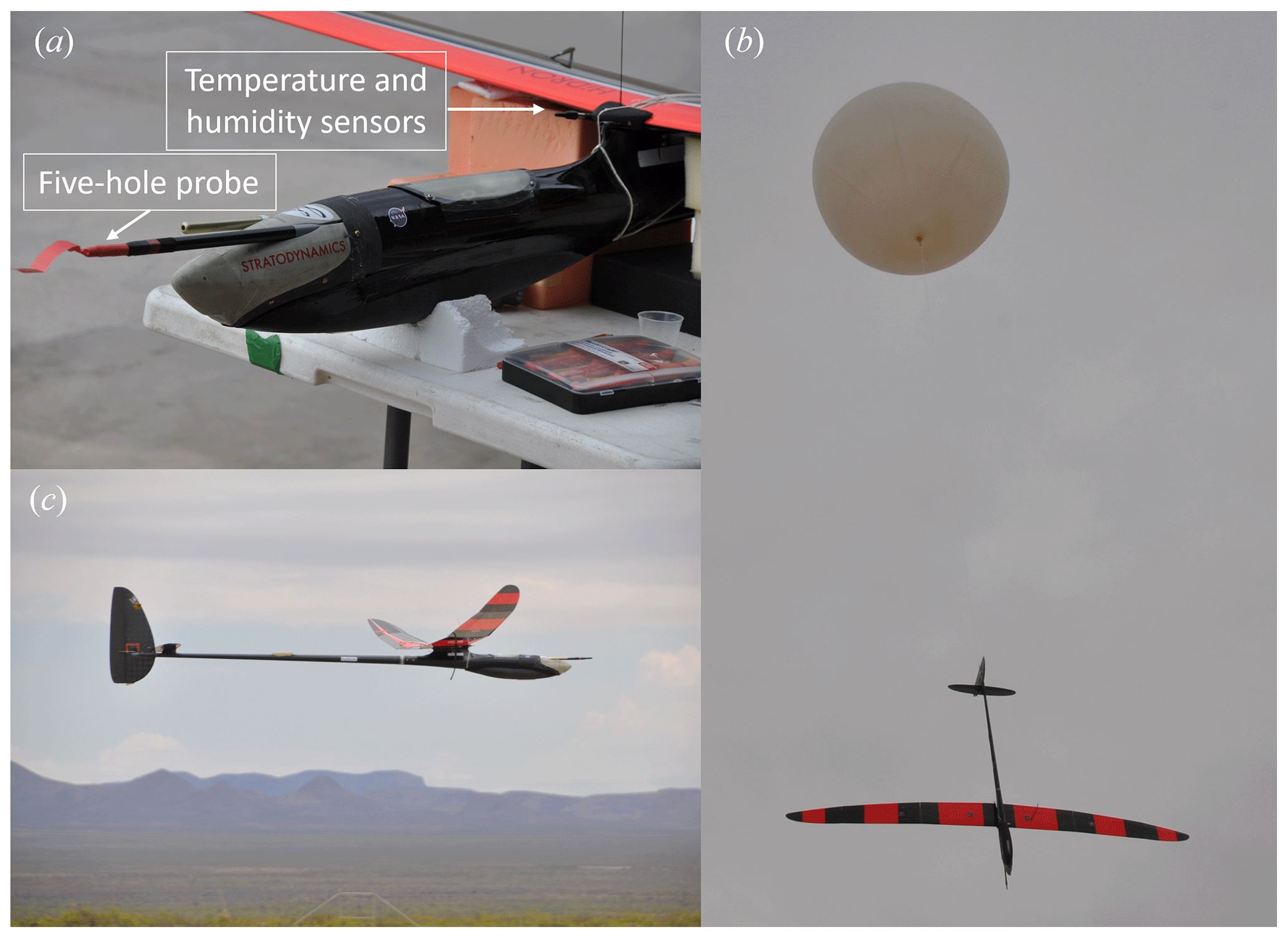
Figure 1Images of HiDRON H2 showing (a) a close-up of the aircraft nose and the locations of the five-hole probe and temperature and humidity sensor, (b) the aircraft during launch, and (c) the aircraft during landing.
Other safety features include a parachute, dual-redundant balloon release system, and geofencing safety protocols that prevent the aircraft from leaving the designated airspace. During prior flights, including flights exceeding altitudes of 30 km, the HiDRON H2 has shown reliability with respect to remaining controllable under high-wind conditions (as high as 32 m s−1), operating under low-temperature conditions (< −60 °C), and returning to a predefined landing site. For the flights reported here, the wind speeds were less than 25 m s−1 and the minimum temperature was −65 °C.
For all flights, the autopilot was set to maintain the aircraft's kinetic energy (reflected through the indicated airspeed), with the value selected near the optimal lift-to-drag ratio (the maximum distance that can be traveled per loss in altitude). To maintain the set airspeed, the autopilot adjusts the pitch angle on the elevator to control the angle of attack of the main wing airfoil. The velocity of the aircraft relative to the air (VR) may therefore fluctuate slightly due to the pitch angle adjustments. Also, as the aircraft descends in altitude, the air density increases and the HiDRON H2's aerodynamic performance improves; thus, VR gradually decreased as the aircraft descended. Figure 2 shows the magnitude of horizontal ground speed (), descent speed (VD) relative to the ground, and the magnitude of the aircraft's velocity relative to the air () for the helical descent portion of each of the three flights as a function of the altitude above sea level. The horizontal velocities are related through , where is the horizontal velocity of the aircraft relative to the ground in the Earth-fixed, inertial frame of reference and e1, e2, and e3 are the basis vectors aligned to the east, north, and up, respectively. The vector is the wind vector and −VDe3 is the aircraft's descent speed in the inertial frame. The method used to obtain the wind velocity vector is provided in Sect. 2.2.
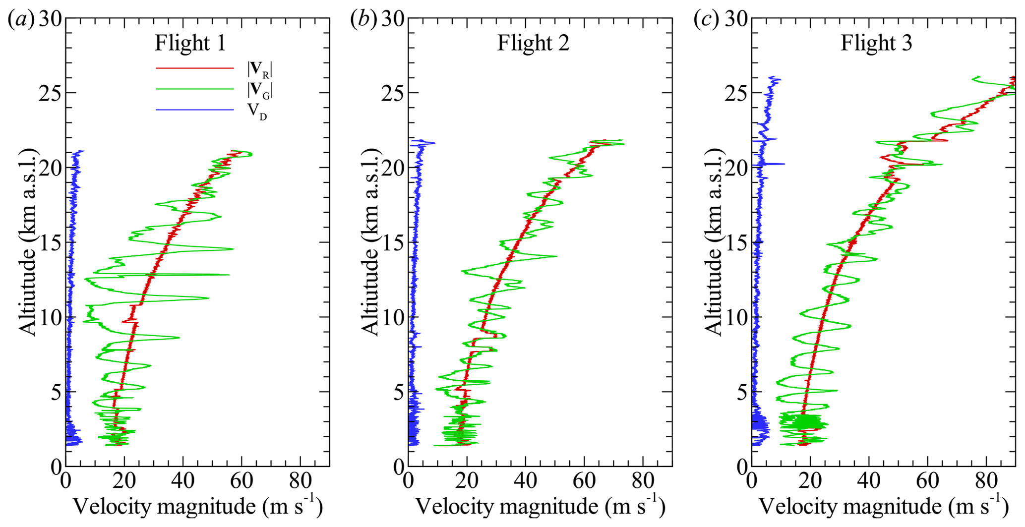
Figure 2Horizontal ground speed in inertial Earth-fixed coordinates (), magnitude of the descent speed in inertial Earth-fixed coordinates (VD), and relative air velocity magnitude in aircraft-fixed coordinates () for (a) Flight 1, (b) Flight 2, and (c) Flight 3.
As noted above, to measure atmospheric conditions, the aircraft was equipped with an integrated InterMet Systems iMet-XF atmospheric sensing system comprising a fast-response bead thermistor to measure air temperature (T) and a capacitive relative humidity (RH) sensor. The manufacturer-provided specifications (International Met Systems, 2023) state that the pressure sensor provided a ± 1.5 hPa accuracy for pressure (P), with the humidity sensor supporting a full 0 %–100 % RH range at a ± 5 % RH accuracy with a resolution of 0.7 % RH. The temperature sensor provided a ± 0.3 °C accuracy with a resolution of 0.01 °C up to a maximum of 50 °C. The stated response times of these sensors are on the order of 10 ms for pressure, 5 s for humidity, and 2 s for temperature in still air, with the autopilot sampling these sensors at 10 Hz. The pressure and temperature sensors were mounted with the sensing elements exposed to the airflow upstream of the wing support (see Fig. 1a) to ensure aspiration of the sensors during forward flight.
2.2 Payload
The turbulence-measuring payload was a combination of four components: (1) a five-hole probe, (2) an infrasonic microphone, (3) a data acquisition board, and (4) an embedded computer. These components were installed in the nose of the HiDRON H2, which could be accessed via removal of the nose cone, as shown in Fig. 3c.
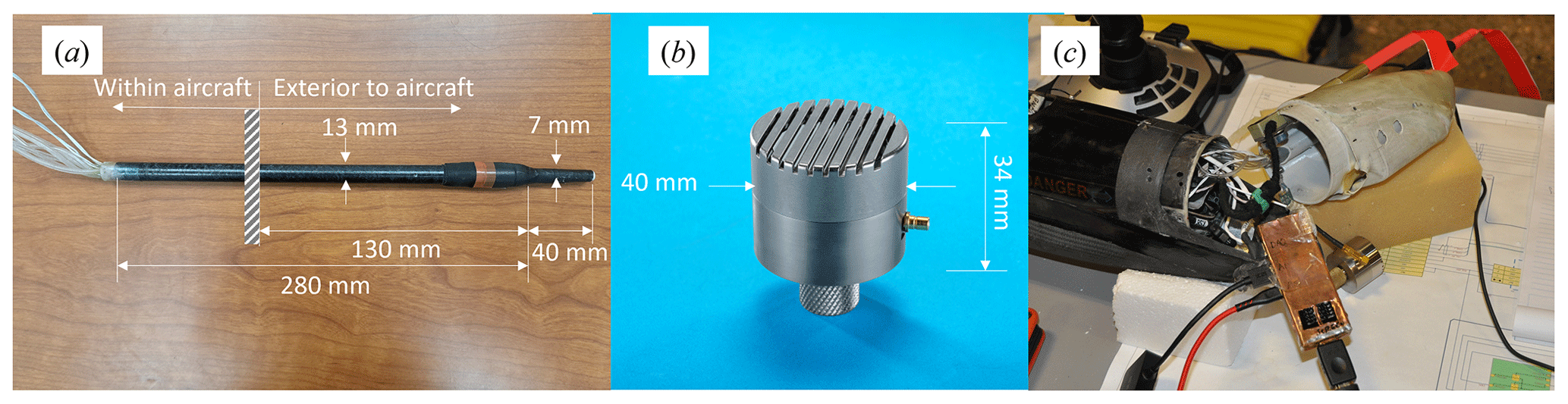
Figure 3The (a) five-hole probe, (b) infrasonic microphone, and (c) nose payload bay open between flights, with the embedded computer shown (removed for data retrieval). The infrasonic microphone is below the embedded computer but was installed in aircraft nose facing forward during flight.
2.2.1 Five-hole probe
Wind speed and direction relative to the aircraft were measured using a bespoke five-hole probe mounted such that the probe projected upstream of the nose of the aircraft, as shown in Fig. 1. The probe, detailed in Fig. 3a, is similar to that used in Bailey et al. (2019, 2020) and Al-Ghussain and Bailey (2022) and was manufactured from a carbon fiber tube equipped with a beveled aluminum tip. The tip of the probe was arranged with one center hole normal to the probe axis surrounded by four other holes arranged symmetrically around it with their plane-normal vector aligned at 20° with respect to the probe axis. For this measurement, the pressure difference between the central hole (measuring total stagnation pressure) and a series of additional holes arranged on the carbon fiber tube (measuring static pressure) was used to determine the approximate dynamic pressure at the probe tip. The pressure measured by this hole combination differs from the true dynamic pressure (Q) depending on the alignment of the wind vector with respect to the probe axis. The two horizontally opposed circumferential holes are arranged to produce a pressure difference which changes with the sideslip angle (β) of the airflow relative to the probe axis. Similarly, the two vertically opposed circumferential holes were arranged to produce a pressure difference which changes with the angle of attack (α) of the airflow relative to the probe axis. Thus, Q, α, and β can be determined by measuring the pressure differences across the different holes arranged on the probe.
Prior to installation on the HiDRON H2, the probe was calibrated in a wind tunnel to determine its directional response using an apparatus designed to pitch and yaw the probe at α and β angles of up to 25° relative to the mean wind vector. Based on established procedures, such as those outlined by Bohn and Simon (1975), Treaster and Yocum (1978), van den Kroonenberg et al. (2008), and Wildmann et al. (2014), and utilizing an implementation approach very similar to that used by Witte et al. (2017), the pressure differences at each α and β angle combination experienced during directional response calibration were used to build pressure coefficients:
where ΔP1 is the pressure difference between the central hole and the static pressure, ΔP32 is the pressure difference across the horizontal probe holes, ΔP54 is the pressure difference across the vertical probe holes, and Q is the dynamic pressure. The probe design resulted in unique combinations of Cβ, Cα, and Cq for each α and β angle of the probe to the relative air velocity vector. These relationships are stored in tables following the wind tunnel calibration.
To calculate the relative wind velocity vector measured during flight, Cα and Cβ were calculated for every sample point from the measured ΔP1, ΔP32, and ΔP54. Using the calibration tables, the values of α and β which produce that combination of Cα and Cβ could be identified. A similar process was used to identify the corresponding value of Cq measured at that Cα and Cβ combination, which allowed Q to be determined. The result is knowledge of the magnitude and direction of the dynamic pressure vector relative to the probe axis for every sampled combination of ΔP1, ΔP32, and ΔP54. The dynamic pressure was then converted to velocity using the density determined from iMet-XF measurements of the ambient pressure, temperature, and humidity.
The probe used on these flights was also heated to prevent ice formation within the probe during flight. This was accomplished by wrapping the probe body in nickel–chromium resistance wire. A feedback circuit, using a thermistor attached to the probe tip, passed current through the wire at a rate sufficient to maintain the probe tip temperature at 50 °C. By repeating the wind tunnel directional response calibrations with and without heating active, it was determined that there was no influence of probe heating on ΔP1, ΔP32, and ΔP54 or on their dependence on α and β. These calibration checks were also conducted at both 20 m s−1, which replicated the expected flight dynamic pressure of Q≈200 Pa, and 5 m s−1, to check for any Reynolds number dependence of Cβ, Cα, and Cq. No evidence of Reynolds number dependence was found.
To measure ΔP1, ΔP32, and ΔP54, the probe was connected to differential pressure transducers through 50 cm of 1.75 mm diameter flexible polymer tubing, specifically Tygon polyvinyl chloride tubing. To ensure that the low-density conditions at flight altitude did not result in pressure differences below the sensitivity of an individual transducer, the measured pressure difference was converted to analog voltage using two different sets of transducers by teeing the tubing to each transducer set, i.e., a low- and high-sensitivity transducer was used for each pressure difference ΔP1, ΔP32, and ΔP54. The low-sensitivity transducer set was comprised of TE Connectivity 4515-DS5A002DP differential pressure transducers with a 500 Pa range. The second transducer set was comprised of All Sensors DS-0368 differential pressure transducers with a 65 Pa range. Both sets of analog output voltages were linearly scaled relative to the maximum transducer range with a nominal span of 4.5 and 4.0 V, respectively. During flight, the autopilot maintained flight speeds sufficient to produce pressure differences well within the range of the low-sensitivity transducers (i.e., the dynamic pressure was maintained between 100 and 200 Pa) which exceeded the range of the high-sensitivity transducer connected to ΔP1. Hence, only the readings from the low-sensitivity sensors were used for data analysis. However, the high-sensitivity ΔP32 and ΔP54 transducers provided a means to estimate the uncertainty in the pressure measurement by comparison with their low-sensitivity counterparts, as will be described later.
To convert the air velocity vector components relative to the probe axis into a frame of reference relative to the ground, an additional coordinate transformation was conducted using the aircraft's pitch, yaw, and roll angles as measured by the autopilot. Details of this process are provided in Witte et al. (2017) and are based on procedures described in Lenschow (1972) for measurements using similar probes mounted on crewed aircraft. This process assumes that the coordinate system of the probe during wind tunnel calibration is perfectly aligned with the body frame coordinate system of the autopilot, which is difficult to achieve in practice. Therefore, an additional procedure was used to correct for any misalignment of the probe axis and the aircraft's body frame axis. This approach, described in Al-Ghussain and Bailey (2021), also corrects for the airframe influence on the measured Q and for time misalignment between the probe's pressure sensors and the aircraft's kinematic sensors.
As the autopilot and payload data acquisition systems were acquired asynchronously, alignment of autopilot kinematic data and five-hole-probe pressure data in time was conducted during post-processing by cross-correlating the dynamic pressure measured by the aircraft's intrinsic pitot probe (recorded by the autopilot along with the aircraft position and orientation information) and ΔP1 of the five-hole probe recorded by the payload data acquisition system. The time lag between the two systems was then removed before performing the transformation of the velocity vector in the aircraft body frame to the Earth-fixed frame of reference. To do so, the aircraft position and orientation information was upsampled from the autopilot's 10 Hz sample rate to the 1 kHz sample rate used by the onboard data acquisition system, with the upsampling conducted using simple linear interpolation.
The result of these procedures is a time-dependent wind velocity vector described using components u(t), v(t), and w(t) which are aligned to the east, to the north, and up, respectively. The time-dependent horizontal wind velocity magnitude and direction could then be found from
and
where atan2 indicates a numerical implementation of the tan −1 function used to disambiguate the polar direction employing the quadrant formed by the sign of the velocity components.
Note also that, although data were acquired at a 1 kHz sample rate to ensure that the infrasonic microphone response was fully resolved, the actual probe maximum frequency response a was much lower due to viscous attenuation of the pressure fluctuations within the tubing, coupled with inaccuracies introduced by high-frequency resonance within the transducer cavity (Grimshaw and Taylor, 2016). Here, the term maximum frequency response is used to indicate the frequency at which there is a −3 dB attenuation in the measured signal relative to the corresponding input being measured. Under ambient conditions, the maximum frequency response of the five-hole probe was estimated to be on the order of 20 Hz using the same measurement approach utilized in Grimshaw and Taylor (2016) and Witte et al. (2017), which measures the response of the system following a step change in pressure. Similar response tests conducted in an environmental chamber at −70 °C and 8000 Pa indicated that, consistent with the model presented in Grimshaw and Taylor (2016), both the resonance in the transducer cavity and viscous attenuation can be expected to increase with altitude, resulting in a slightly lower maximum frequency response of 10 Hz.
Figure 4a shows an example of the intrinsic electrical noise observed in the pressure transducer signals. Although this particular excerpt was measured from the low-sensitivity ΔP1 transducer during the environmental test at −70 °C and 8000 Pa, similar signals were measured by the other pressure transducers under ambient conditions; during environmental testing; and during flights 1, 2, and 3. The electrical noise was found to be composed of a 2 Pa stochastic component combined with a −8 to 0 Pa quasiperiodic component. As similar characteristics were observed for both the low- and high-sensitivity transducers, scaling with the range of the transducers, it is hypothesized that this noise is introduced through the common 5 V reference signal used to power all pressure transducers. As shown in Fig. 4b, which compares the one-sided autospectral density, FPP(f), calculated from 5 min of the low-sensitivity ΔP1 transducer time series measured during the environmental chamber test under ambient conditions to an equivalent measurement made at −70 °C and 8000 Pa, the frequency content of this noise signal was independent of ambient pressure and temperature conditions. Furthermore, Fig. 4c shows the equivalent autospectral density calculated from a quiescent period of the Flight-1 low-sensitivity ΔP1 time series in red, specifically from a 5 min portion of the time series while the aircraft was on the ground prior to launch. This autospectral density shows that a similar energy content to that measured in the environmental chamber was also present during the flight tests. Also shown in Fig. 4c is the frequency content measured during every 5 min segment of the ΔP1 time series during the controlled-descent portion of Flight 1. Although the low-frequency content of the signal produced FPP(f) values up to 4 orders of magnitude higher than the intrinsic noise, at frequencies higher than the maximum frequency response of the five-hole probe (specifically when f > 100 Hz), the frequency content of the signal remained independent of ambient conditions.
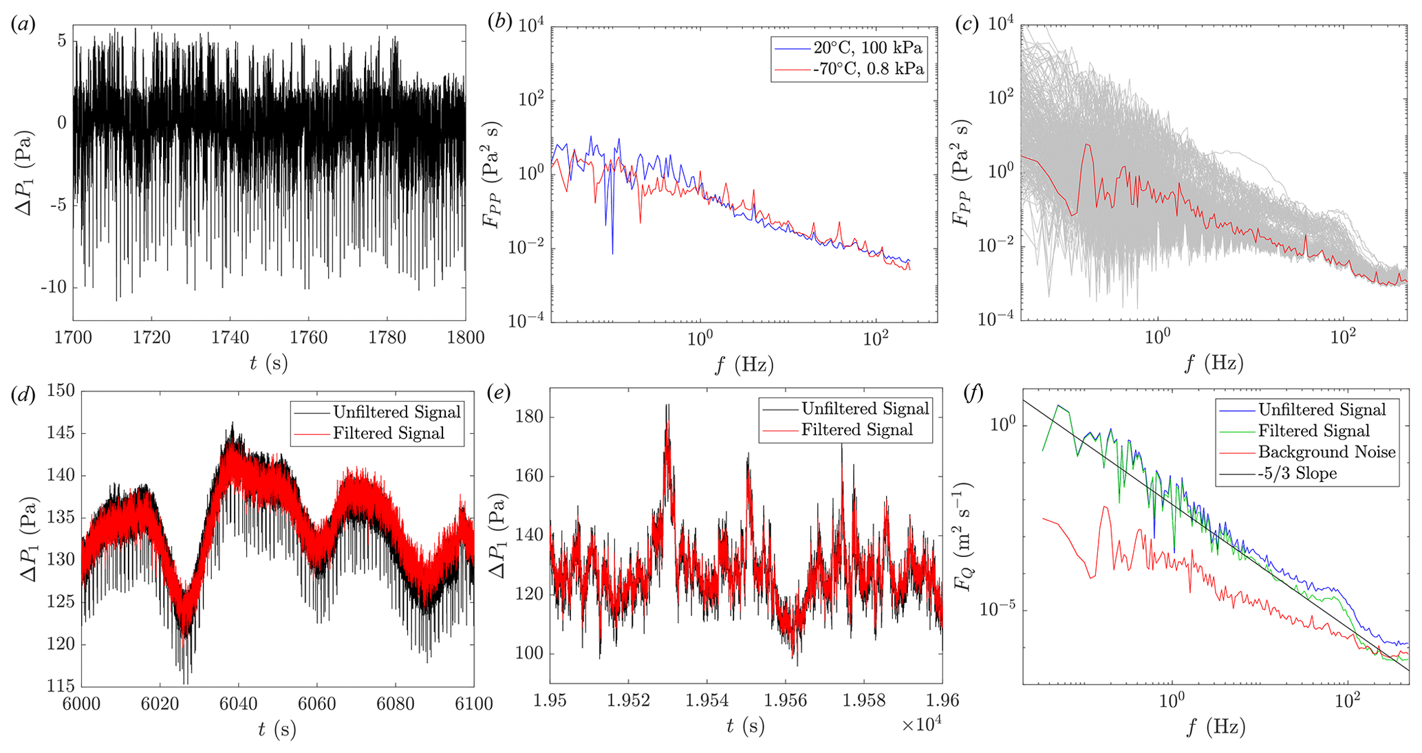
Figure 4(a) Time series showing the intrinsic electrical noise in the pressure transducer signal measured during an environmental test at −70 °C and 8000 Pa. (b) One-sided autospectral density from same test comparing the frequency content in the ΔP1 transducer from 5 min periods under ambient conditions and −70 °C and 8000 Pa. (c) One-sided autospectral density from the ΔP1 transducer measured during a quiescent 5 min period before launch, shown in red, compared to one-sided autospectral density calculated from same transducer's time signal for every 5 min period during the controlled descent of HiDRON H2. Comparison of time series from the ΔP1 transducer measured before (unfiltered signal) and after (filtered signal) the noise removal process during Flight 1 (d) while the HiDRON H2 was in the stratosphere and (e) while the HiDRON H2 was in the atmospheric boundary layer. (f) Comparison of one-sided autospectral density of the measured while aircraft was in atmospheric boundary layer with and without noise removal applied along with corresponding background noise for comparison. Also presented in panel (f) is a solid line showing the slope.
To minimize any possible impact of this electrical noise on the statistical analysis of the five-hole-probe measurements, a background noise subtraction procedure was conducted during post-processing. This procedure filtered the voltage signals by subtracting the background noise energy content in the frequency domain prior to scaling the voltage to pressure. For this purpose, a 5 min segment of each pressure transducer signal measured before balloon launch was chosen, specifically when the probe's cover was installed (as depicted in Fig. 1a). This portion of the time series was assumed to be representative of the background electrical noise. The amplitude of its Fourier transform was subtracted from the corresponding Fourier-transformed voltage signal in 5 min intervals while also preserving the phase information of the original segment. The filtered signal was then returned to the time domain by conducting an inverse Fourier transform.
A 100 s long segment of the original, unfiltered, low-sensitivity ΔP1 time series is shown in Fig. 4d from a portion of Flight 1 during which the HiDRON H2 was within the stratosphere, when the frequency content of the signal was small. Also shown in this figure is the same segment of the time series following the frequency domain filtering described above. The comparison indicates that the filter was successful with respect to removing the quasiperiodic contribution of the noise; however, due to its stochastic nature, the low-amplitude ±2 Pa contribution to the electrical noise remains. A similar comparison is provided in Fig. 4e from a portion of the ΔP1 time series measured when the HiDRON H2 was within the turbulent boundary layer during Flight 1. This figure illustrates that, under conditions in which there is significant frequency content in the signal, this content is preserved during the filtering process. This last point is perhaps better illustrated in Fig. 4f, which shows the one-sided autospectral density, FQ(f), of the frequency content of (which approximately corresponds to the magnitude of the air velocity relative to the probe), measured within the boundary layer during Flight 1 with and without the filter applied. Figure 4f illustrates how the low-frequency (f < 1 Hz) content of the measured signal is largely unaffected by the filtering process, with the filter impact increasing as the energy within the signal decreases at higher frequencies. Also illustrated in Fig. 4f is how application of the filter increases the agreement of the frequency-dependent roll-off of FQ(f) with the dependence expected for inertial subrange turbulence. The broadband peak in FQ(f) evident at f ≈ 100 Hz is attributed to resonance within the transducer cavity, as it is not present in the background noise FQ(f) spectrum.
It should be noted that ignoring the phase information of the background noise during the removal process could introduce artifacts into the time domain of the filtered signal, particularly when the amplitudes of the signal and subtracted background noise are similar (e.g., at high frequencies and when the air is quiescent). By comparing the statistics presented in Sect. 3 with and without the filtering applied, we find that the primary benefit of implementing this background noise subtraction process is that it reduces some of the scatter in the data, allowing trends to become more evident. However, caution has been exercised when interpreting results in which the distortion of the signal is likely.
Finally, the ΔP54 pressure line was inadvertently disconnected during maintenance prior to flights 2 and 3 and not discovered until after Flight 3. Therefore, for these flights, conversion of the five-hole-probe voltages was conducted with α provided by the autopilot's telemetry data. This α was estimated from the true airspeed determined from the aircraft's pitot probe, which measures the relative air speed along the aircraft's longitudinal axis, and the speed of the aircraft through the air along the aircraft's vertical axis. This latter speed was determined using the aircraft's descent rate, which itself was estimated through a Kalman filter fusion of the static pressure rate of change, vertical acceleration, and global positioning system (GPS) velocity. By assuming that the relative vertical component of the velocity of the air to the aircraft was only due to the descent rate of the aircraft through the air, the speed in the aircraft's vertical axis could then be determined by combining the aircraft's descent rate and true airspeed information with the aircraft orientation measured by the autopilot gyroscopes. The latter information allowed transformation from inertial to body-fixed coordinates. The definition of Cα and Cβ used for directional calibration and recovery of Q and β were also modified to not include ΔP54. While not ideal, we were able to verify that this approach was justified by processing the Flight-1 data with and without the inclusion of ΔP54. The average difference between the resulting u(t), v(t), and w(t) values was found to be less than 0.25 m s−1, with the average difference in the Reynolds normal stresses found to be less than 0.09 m2 s−2. Importantly, the altitude dependence of these quantities was preserved. Figures comparing the differences resulting from the processing methods are presented in Appendix A.
2.2.2 Infrasonic microphone
Infrasonic measurements of acoustic frequencies were conducted using an infrasonic microphone. For these tests, a microphone and acoustic measurement system developed at NASA Langley Research Center was used. The microphone, shown in Fig. 1b, when coupled with a PCB Piezotronics 485M49 amplifier, was capable of infrasound (acoustic frequencies lower than 20 Hz) detection with a sensitivity of 115 mV Pa−1 (amplified to ± 10 V); this system had a power consumption of 35 mW and a weight of 186 g. The geometry of the 38.1 mm diameter microphone diaphragm was designed with a high compliance (low diaphragm tension) such that membrane motion was substantially critically damped and optimally dimensioned for the 0.01 to 20 Hz frequency range, with the full bandwidth of the sensor being 0.01 Hz to 1 kHz.
The microphone was mounted rigidly within the nose of the aircraft with the diaphragm plane normal to the forward flight direction. By being located within the fuselage, the microphone was protected from dynamic pressure fluctuations. As the wavelengths of infrasonic sound exceed 10 m, sound attenuation by the fuselage was not expected for frequencies lower than 20 Hz.
2.2.3 Data acquisition
A Measurement Computing Systems MCC USB-1608FS-Plus data acquisition system (DAQ) was used to digitize the voltage output from the pressure transducers and microphone signal conditioning unit. The DAQ also provided the 5 V signal used to power the pressure transducers. This particular DAQ was capable of recording eight single-ended analog inputs simultaneously at 16-bit resolution at rates of up to 400 kHz. During these experiments, the DAQ sampled (at 1 kHz) the seven channels containing the analog voltage signals from all six pressure transducers and the infrasonic microphone. Digitized voltage values were then transferred through universal serial bus to the embedded computer for logging.
2.2.4 Embedded computer
The DAQ was connected, via universal serial bus (USB), to a mini stick computer with an Intel Atom Z8350 processor, 128 GB eMMC non-volatile memory, and 4 GB RAM. To minimize radio frequency interference and shield the computer from high-altitude radiation, the computer was encased in a copper shield (Fig. 3c). A custom script was used to control data acquisition and storage. The computer stored all recorded data on its eMMC memory; these data were then downloaded post-flight via USB connection for archiving and further analysis. To allow payload operational verification during flight, an RS232 connection was established between the computer and the autopilot. Through this channel, sensor voltage variance and preliminary turbulence detection parameters were passed to the autopilot to be included in the telemetry stream. This information was also later available for preliminary temporal alignment of sensor and autopilot data.
2.3 Uncertainty estimation of wind measurement
As described above, measurement of the wind vector was a multistep process involving information from different sensors, calibrations, and corrections. Therefore, to assess the uncertainty in the wind vector measurement, a Monte Carlo method was used to estimate the error propagation from the sensors to the final wind estimate. To do so, the post-processing calculations were repeated for 100 iterations with each iteration having the sensor values perturbed from their measured value by an amount determined using normally distributed random number generators. The standard deviation of the normal distributions were selected to correspond to each sensor's uncertainties.
Specifically, for a measured sensor value, here represented as Φ(t), a perturbed value, Φi(t), was found for each iteration, i, following
where 𝒩 represents a normally distributed random number drawn from a standard normal distribution with a mean of zero and standard deviation of unity. The quantities EB and EP represent the respective estimated bias (accuracy) and precision (resolution) errors for the sensor being perturbed, with the bias error perturbation, 𝒩, added to Φ(t) only once per iteration, and the precision perturbation, 𝒩(t), added for every sample in time. Here EB and EP are taken to represent the 95 % uncertainty range, twice the standard deviation of their distribution.
The analysis produced an ensemble of 100 time-dependent (and hence altitude-dependent) measurements of wind for each flight, randomly distributed via the propagation of the perturbed sensor readings, each perturbed following Eq. (11). The uncertainty estimate was then found for the magnitude and direction from twice the ensemble standard deviation at each measurement time (t), corresponding to a 95 % probability, of the 100 iterations. Note that this approach is similar to that employed by van den Kroonenberg et al. (2008); however, by employing the Monte Carlo analysis, the approach in this work allows the uncertainty to vary in time (and hence altitude) as well as incorporating any additional uncertainty which may occur due to coupling of sensor errors.
The values for EB and EP used in the uncertainty propagation analysis are provided in Table 1 and required different methods for their determination. For the pressure differences measured by the transducers connected to the five-hole probe (ΔP1, ΔP32, and ΔP54), EB was estimated from the average difference between the low-sensitivity and high-sensitivity ΔP32 and ΔP54 transducer values recorded during each flight, whereas EP was estimated using twice the standard deviation of the difference. For P, T, and RH, the manufacturer-provided accuracy and resolution values were used for EB and EP, respectively. Finally, the uncertainty in the attitude and heading reference system (AHRS) used by the autopilot was not available, so the accuracy and resolution values from a different manufacturer's equivalent AHRS system were used as proxy values.
Table 1Bias and precision errors for each sensor value used in the wind estimate.
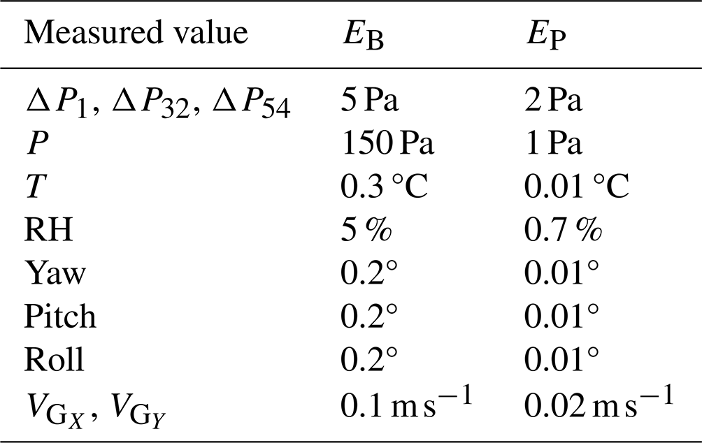
Note that this analysis does not consider additional uncertainty introduced by errors in the directional calibration, misalignment in time between the sensors, and any altitude-dependent variability in the values provided in Table 1. To accommodate these undetected uncertainties in the analysis, the EB and EP values provided in Table 1 were doubled prior to implementation in Eq. (11).
The mean value of U across the 100 iterations at each time step is shown in Fig. 5a, b, and c for flights 1, 2, and 3, respectively, along with the corresponding 95 % (2-standard-deviation) uncertainty bounds. The resulting uncertainty in the wind estimate was found to be altitude dependent, with the highest uncertainty of approximately 3.5 m s−1 observed at the highest altitudes, decreasing to approximately 0.5 m s−1 at the lowest altitudes measured. This altitude dependence directly arises from the influence of P, T, and RH uncertainty on the air density estimate. The magnitude of the uncertainty presented in Fig. 5 is consistent with the results of an intercomparison study presented in Barbieri et al. (2019). In this intercomparison, wind estimates from probes and procedures very similar to that used here were found to be within ± 1 m s−1 of a ground-based reference velocity sensor.
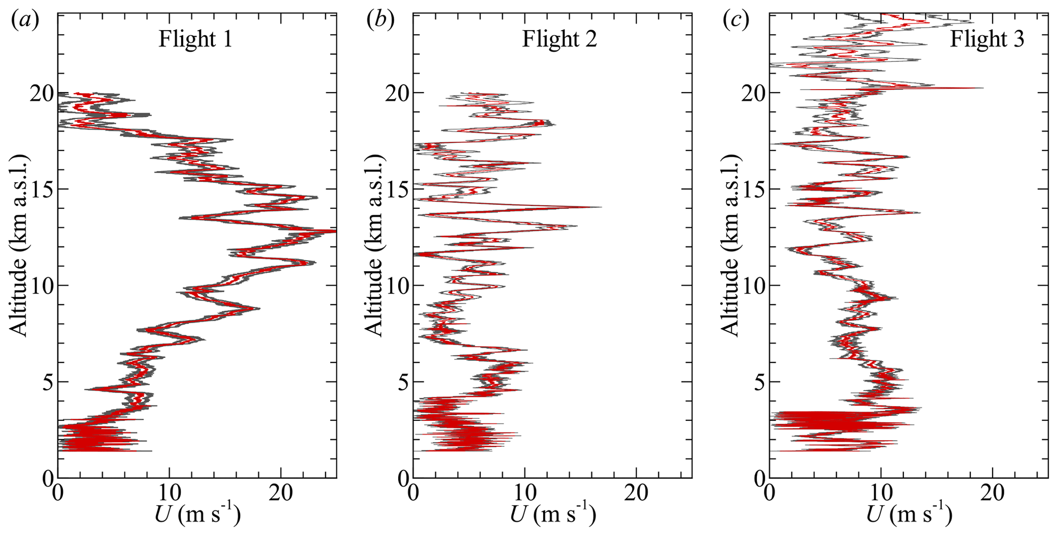
Figure 5Result of the uncertainty analysis for (a) Flight 1, (b) Flight 2, and (c) Flight 3. Red lines show the velocity magnitude calculated from the mean of 100 ensembles, with the corresponding 95 % uncertainty bounds shown as black lines.
Furthermore, although not directly apparent in Fig. 5, the uncertainty in the wind magnitude was found to be most dependent on the yaw angle, which is consistent with the observations of van den Kroonenberg et al. (2008). This is due to the dependence of wind magnitude on aircraft yaw, pitch, and roll introduced during the coordinate transformation between the body-fixed and inertial coordinate systems. During flight, the yaw angle can vary from 0 to 360°, whereas the α, β, pitch, and roll angles are near 0°. The result is that, during the coordinate transformation, the u and v wind components are primarily determined from the true airspeed multiplied by the sine of the yaw angle and the cosine of the pitch angle for u and by the cosine of the yaw angle and the sine of the pitch angle for v (e.g., van den Kroonenberg et al., 2008). Thus, during an orbit, the horizontal velocity components will have the highest sensitivity to error in the aircraft's yaw angle, both at yaw angles of 0° (for u) and 90° (for v) which, for a helical flight path (such as that flown in this study), can introduce periodic artifacts into the wind estimates. The vertical component of the wind velocity (w) is most sensitive to error in the pitch angle due to this component of wind being primarily determined by the true airspeed multiplied by the sine of the pitch angle (which is near 0° for most of the flight).
2.4 Experiment overview
The aircraft–payload combination was deployed in a measurement campaign conducted in the restricted airspace above Spaceport America, located near Truth or Consequences, New Mexico, USA, between the Black Range and the San Andres Mountains (Fig. 6), from 1 through 6 June 2021. The height of aircraft launch and recovery was 1406 Three flights were conducted by the HiDRON H2 on different dates, with Flight 1 being conducted on 1 June, Flight 2 being conducted on 4 June, and Flight 3 being conducted on 6 June. Each flight consisted of a weather balloon carrying the glider aloft at an ascent rate of approximately 7 m s−1 to a release altitude of 25 for flights 1 and 2 and a release altitude of 30 for Flight 3, corresponding to z = 23.6 km and z = 28.6 (above ground level), respectively. After release from the balloon, the aircraft conducted an automated descent along a predetermined flight path towards the Spaceport America runway. Autopilot-controlled approach, landing, and recovery occurred on the Spaceport America main runway, at which point the aircraft, payload, and all logged data were recovered.
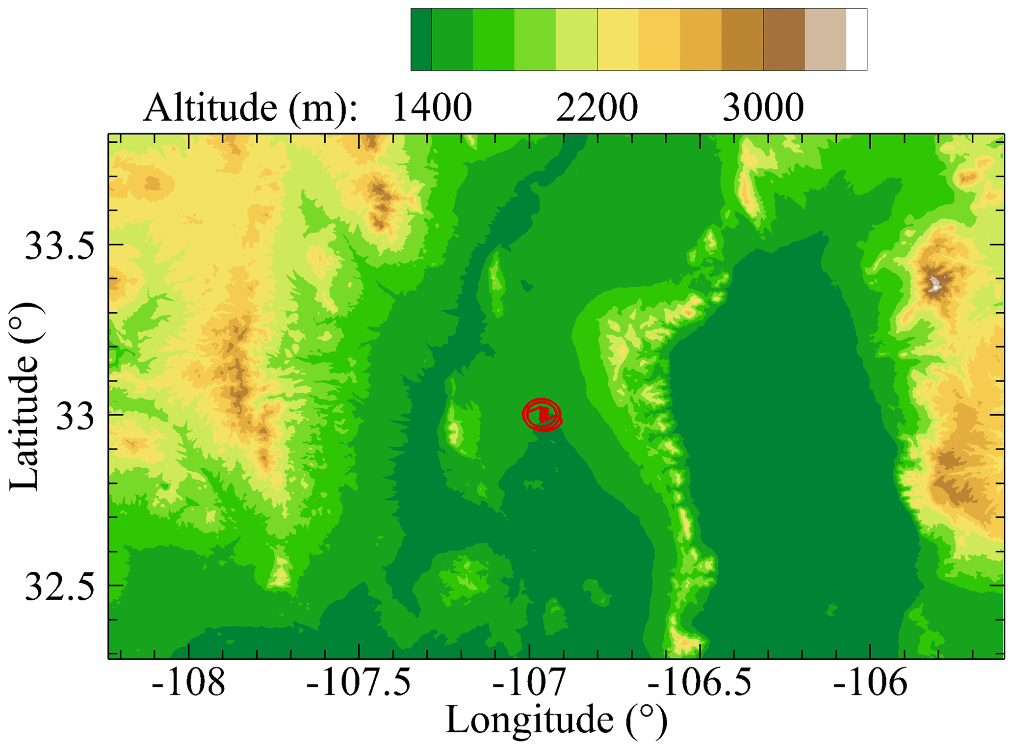
Figure 6The topography of the flight area over Spaceport America with the trajectory of Flight 3 indicated by a red line to illustrate the region of measurement.
2.5 Flight profiles
The flight trajectories for all three flights are presented in Fig. 7, which shows balloon launch, ascent to 25 or 30 altitude, release of the HiDRON H2 aircraft, controlled return to the airspace above the launch and control point, and helical descent to the landing point. The helical descent was conducted at an initial radius of approximately 5 km, which was selected as a compromise between optimizing the aerodynamic efficiency of the aircraft in a turn (by minimizing the bank angle) and remaining in close proximity to the landing runway. As the aircraft descended, this radius was reduced to approximately 4 km and, eventually, 1 km to keep the aircraft within gliding distance of the designated landing point. During the descent phase of the flight, as shown in Fig. 2, the rate of descent decreased from 5 to 1 m s−1 (producing a nominal descent rate of 2 m s−1). Overall flight time was approximately 6 h, with 4 h of that being the descent phase. Note that, during descent, several tests were conducted of the HiDRON H2's flight control system (including a test of autonomous soaring during Flight 3 which resulted in the aircraft gaining altitude for approximately 10 min). The result of these tests were occasional deviations of the flight path from the nominal helical trajectory.
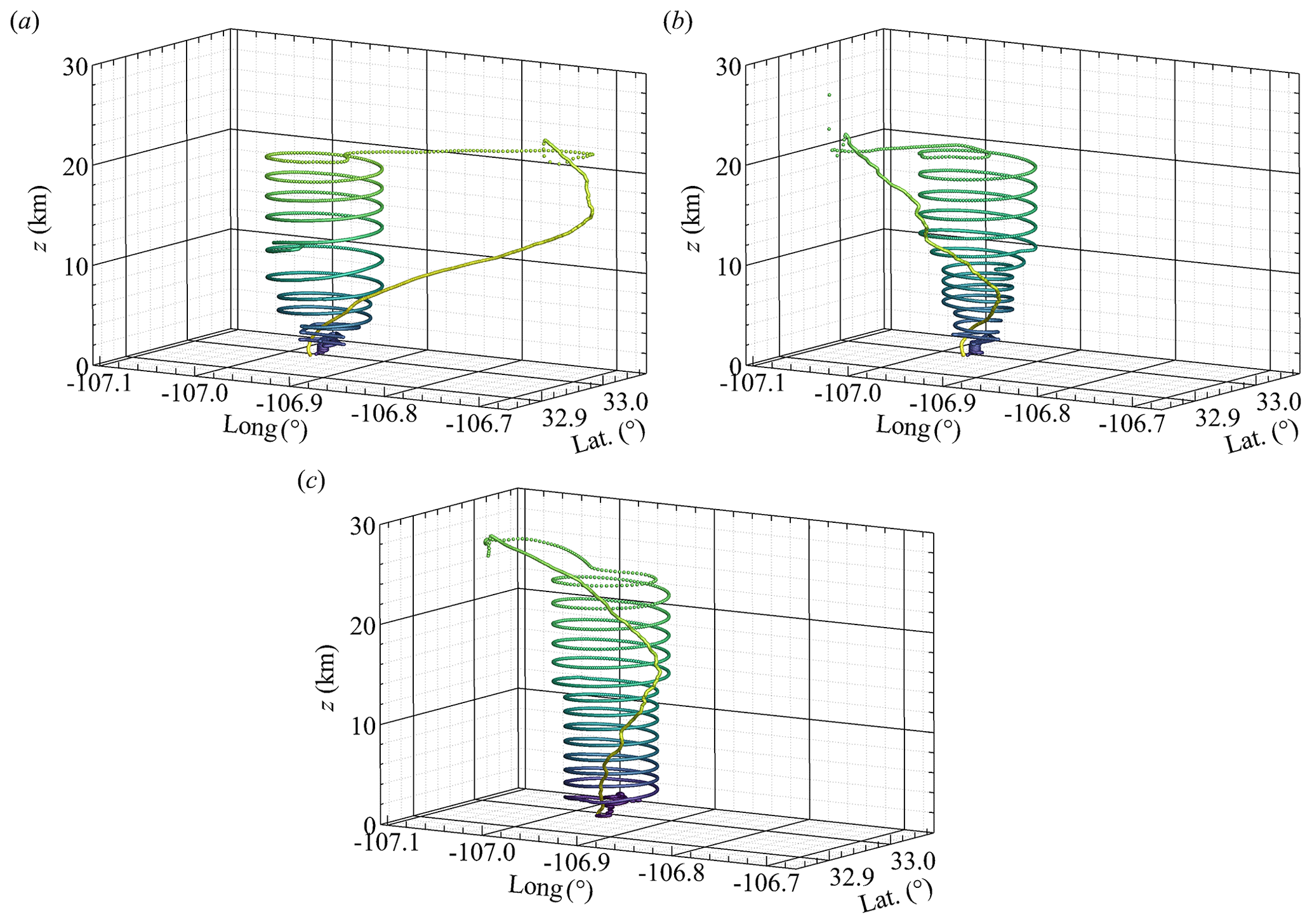
Figure 7HiDRON H2 flight trajectory for (a) Flight 1, (b) Flight 2, and (c) Flight 3. The trajectory is colored by time, with a lighter color indicating the earliest phase of the balloon ascent. z indicates height above ground level.
All three flights started in the morning hours. Flight 1 launched at 13:47 UTC (coordinated universal time; 07:47 LT, local time) on 1 June 2021, released from the balloon at 14:35 UTC (08:35 LT), and landed at 18:42 UTC (12:42 LT). Flight 2 launched at 14:04 UTC (08:04 LT) on 4 June 2021, released at 15:15 UTC (11:15 LT), and landed at 18:39 UTC (12:39 LT). Finally, Flight 3 launched at 14:07 UTC (08:07 LT) on 6 June 2021, released at 15:17 UTC (09:17 LT), and landed at 19:43 UTC (13:43 LT). Local time (LT) at Spaceport America was mountain daylight time (UTC−6:00).
In this section, we present the measured values of temperature, relative humidity, wind vector, and infrasonic microphone signal amplitude, as well as presenting the calculation approaches and results for selected statistics. The temperature and humidity sensors were mounted on the front side of the wing support pillar (as shown in Fig. 1a); thus, during ascent, they were in a stagnant region within the wing pillar wake and not sufficiently aspirated to prevent self-heating and delayed air exchange with the environment. Hence, only data from the controlled-descent phase of the flight are presented for temperature and humidity in this section. Here, z is used to indicate the vertical distance referenced to ground level, i.e., above ground level (), with z=0 corresponding to the launch and recovery altitude of 1406 In addition, when presenting results measured during descent, we limit the data to z < 20 km for flights 1 and 2 and to z < 25 km for Flight 3, i.e., the portion of the flight during which the aircraft was following a the helical trajectory (see Fig. 7), and within ± 5 km of a fixed geographic location. This latter constraint is introduced because even the low-sensitivity ΔP1 exceeded the transducer's range shortly after the aircraft was released and started its flight towards the helical orbit location. By the time the aircraft reached the orbit location, ΔP1 had returned to a range measurable by the low-sensitivity transducer, although it never reduced to a value measurable by the high-sensitivity ΔP1 transducer.
The time series of U(t) measured during descent is presented in Fig. 8a. For this figure, the time series has been filtered using a low-pass filter at 1 Hz to better visualize some of the features of the time series. By inspection, it was observed that, while the aircraft was in the stratosphere (t < 7000 s), the velocity fluctuations were largely composed of low-frequency motion with periods on the order of 400 s, as illustrated in the segment of the time series shown in Fig. 8b. For the nominal of approximately 60 m s−1 in this altitude range (see Fig. 2), this corresponds to wavelengths on the order of 24 km. Interspersed with these low-frequency motions were irregular occurrences of high-frequency fluctuations more characteristic of turbulence, such as that shown in Fig. 8b around t = 6000 s. These latter events occurred in bursts lasting on the order of 100 s (or 6 km). As the aircraft descended through the troposphere, similar behavior was observed, although the duration of high-frequency events was typically longer, on the order of 300 s (as illustrated in Fig. 8c around t = 12 000 s and t = 12 500 s). However, 20 m s−1 at these altitudes, so the corresponding lengths of these events remained near 6 km. Towards the end of the flight, the intensity and frequency of the high-frequency occurrences increased (Fig. 8d), consistent with the UAS approaching and entering the boundary layer (t > 16 500 s). Similar behavior was observed for flights 2 and 3.
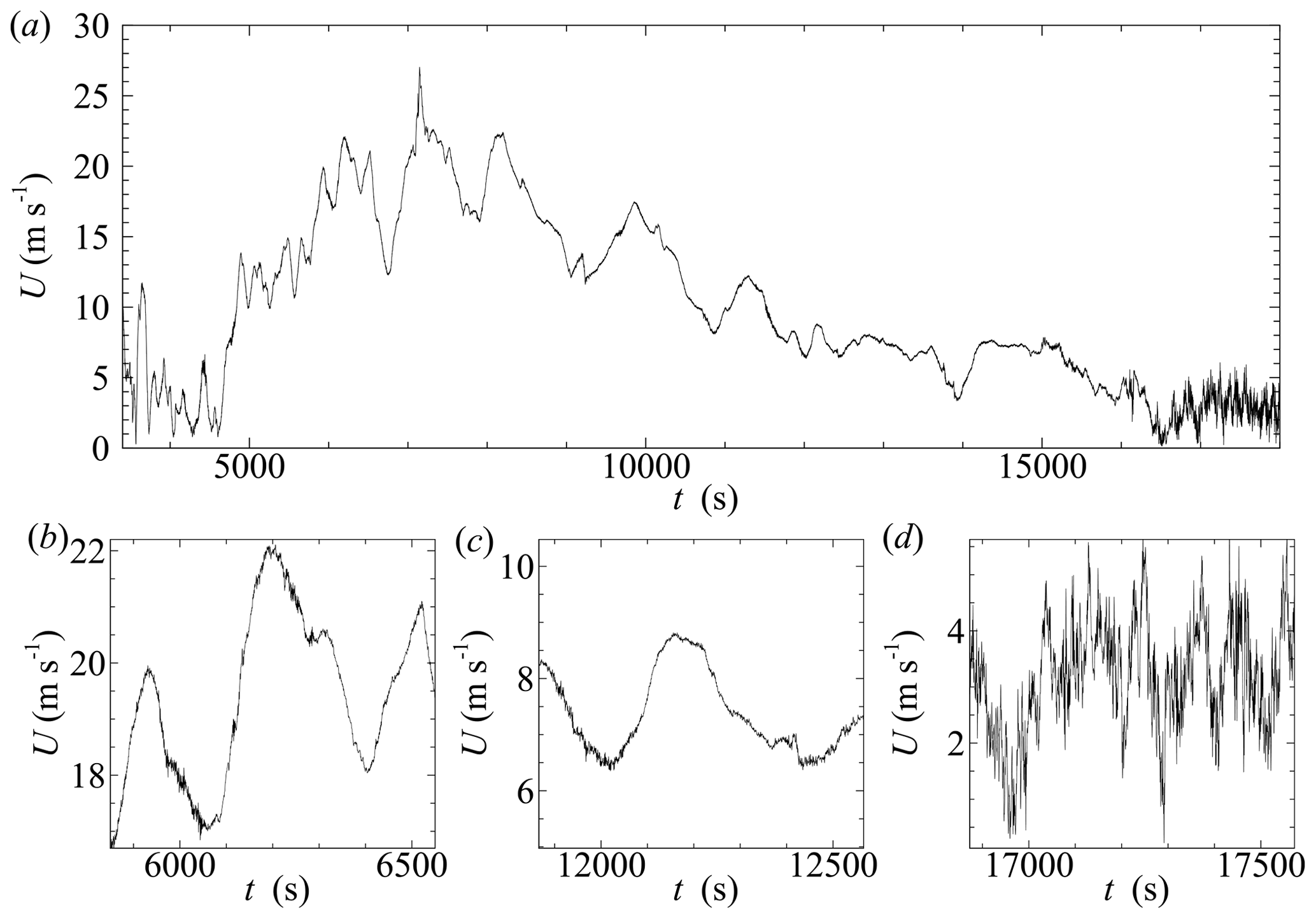
Figure 8Time series of the low-pass-filtered (at 1 Hz) velocity magnitude for (a) a controlled-descent portion of Flight 1, with t=0 corresponding to the startup of the data acquisition system prior to balloon release. Panels (b), (c), and (d) show selected portions of time series in the stratosphere, troposphere, and boundary layer, respectively.
Following these observations, to capture the statistical properties of the high-frequency portions of the time series, the descent portion of the flight was divided into 3 km statistical segments, determined using , where Δt is the amount of time included in each segment. Due to the spiralling flight path (as illustrated in Fig. 7), each 3 km segment represents approximately 150 m of vertical descent. Quantities averaged over these segments are displayed using angle brackets, 〈 〉. In order to decrease the vertical spacing between statistical values, each segment is overlapped with its neighbor by 50 %, thereby decreasing the spacing of statistical quantities to 75 m vertically. Finally, to minimize the effects of low-frequency bias on the statistics calculated for each segment, when statistics require the subtraction of a local mean value, e.g., as required to determine u′(t), v′(t), or w′(t), we subtract the linear trend within that segment (i.e., by detrending the segment), rather than subtracting the segment's mean value.
3.1 Mean quantities
To establish the ambient conditions during each flight, we averaged P, T, RH, U, and γ over each statistical segment and compared the vertical profiles of these quantities to publicly available 12:00 UTC National Weather Service (NWS) radiosonde weather soundings launched from the El Paso (EPZ), Albuquerque (ABQ), and Tucson (TUS) NWS forecast offices. These forecast offices and sounding times were selected due to their proximity to the launch site and flight times, with the launch site within the triangle formed by these three locations. To assist with comparison across sites in z, we have set z=0 at 1406 for all soundings. Furthermore, to assist with comparison, the National Oceanic and Atmospheric Administration (NOAA) upper-air maps at 250 mbar and National Aeronautics and Space Administration (NASA) satellite imagery for the approximate time of flights 1 through 3 are provided in Appendix B with the NWS sounding sites and Spaceport America (SPA) indicated on them. The NWS soundings employed Graw DFM-17 radiosondes with manufacturer-provided accuracies of ± 0.2 °C for temperature, ± 4 % for RH, ± 0.1 m s−1 for wind speed, and ± 1° for wind direction.
Vertical profiles of 〈T〉 and 〈RH〉, measured by the HiDRON H2, are compared to the radiosonde profiles for all three flights in Fig. 9. The HiDRON H2 temperature is consistent with the trends produced by the radiosonde values, although it shows a noticeable warm bias compared with the radiosondes for z = 16 km that most evidently appears in the results from Flight 3. Note that no density or other correction was applied to this sensor measurement to account for the reduced convective heat transfer at these altitudes. The lapse rate in the troposphere also appears to deviate from the radiosonde lapse rates for z < 5 km, although it is not clear if this is due to a sensor-related issue or to spatial variability in the atmospheric conditions.
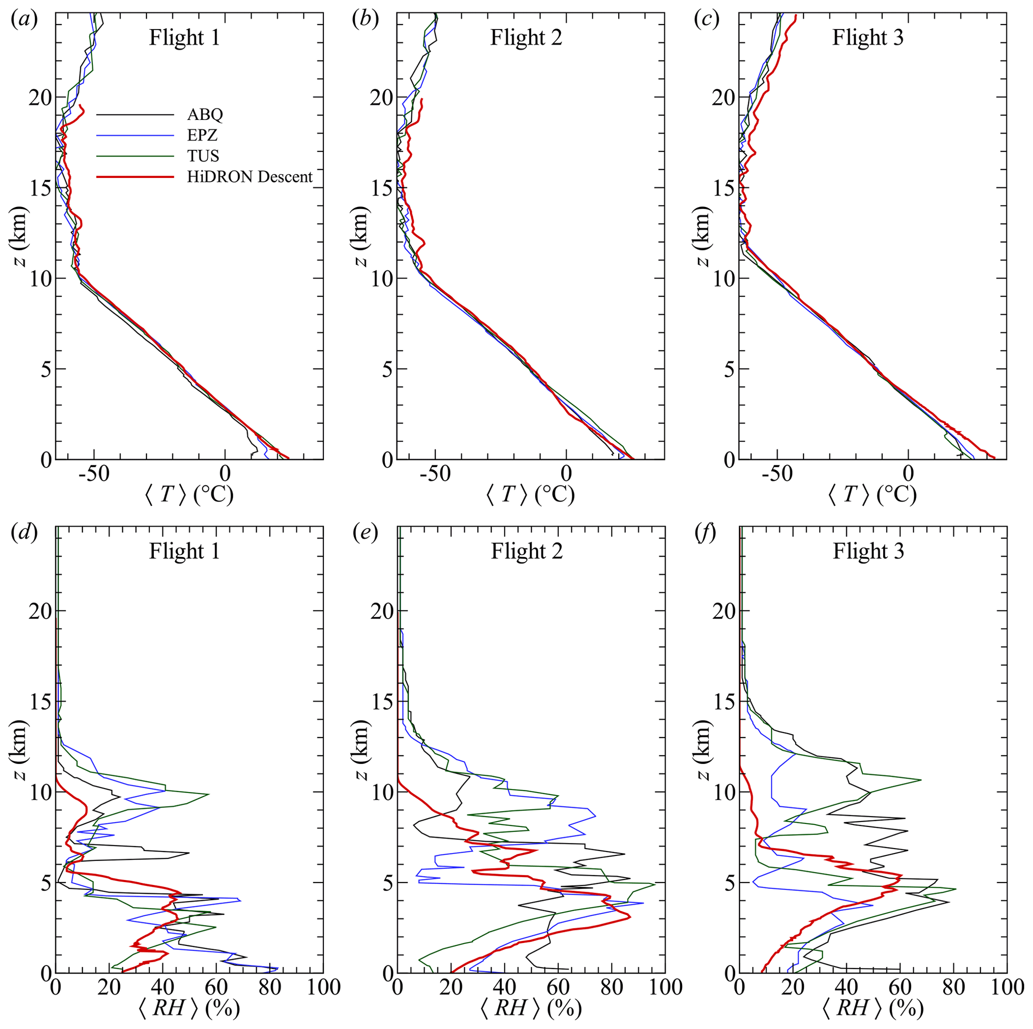
Figure 9Temperature profiles measured during (a) Flight 1, (b) Flight 2, and (c) Flight 3 compared to NWS radiosonde soundings from the Albuquerque (ABQ), El Paso (EPZ), and Tucson (TUS) forecast offices. Corresponding relative humidity profiles are shown for (d) Flight 1, (e) Flight 2, and (f) Flight 3.
Figures 9d, e, and f compare the corresponding 〈RH〉 measurements from the HiDRON H2 and NWS radiosondes. Significant differences are clearly evident among the profiles. However, noting that the radiosonde data were obtained from disparate locations up to 380 km away from the flight location, differences can be attributed to spatial heterogeneity in the atmospheric moisture concentration. This is qualitatively illustrated by comparison of the cloud coverage in satellite observations (Appendix B). However, on all 3 d, the HiDRON H2 reported consistently lower RH values for z > 7 km, so a dry bias in the humidity sensor under cold conditions cannot be discounted.
The magnitude and direction of the horizontal winds for all three flights are shown in Fig. 10. In addition to comparison to the radiosonde soundings from ABQ, EPZ, and TUS, we also compare the profiles measured during descent to those estimated from the ascent phase of each flight using as measured by the autopilot's GPS. To mitigate any possible influence of pendulum motion of the aircraft on the balloon tether (estimated to have a natural period of approximately 5 s), the velocity values were filtered by applying a 25 s moving average. The resulting wind estimates are treated as approximately equivalent to those produced by radiosondes, although the significantly increased weight of the aircraft relative to a radiosonde can be expected to produce a corresponding increase in the time constant compared with that of a radiosonde.
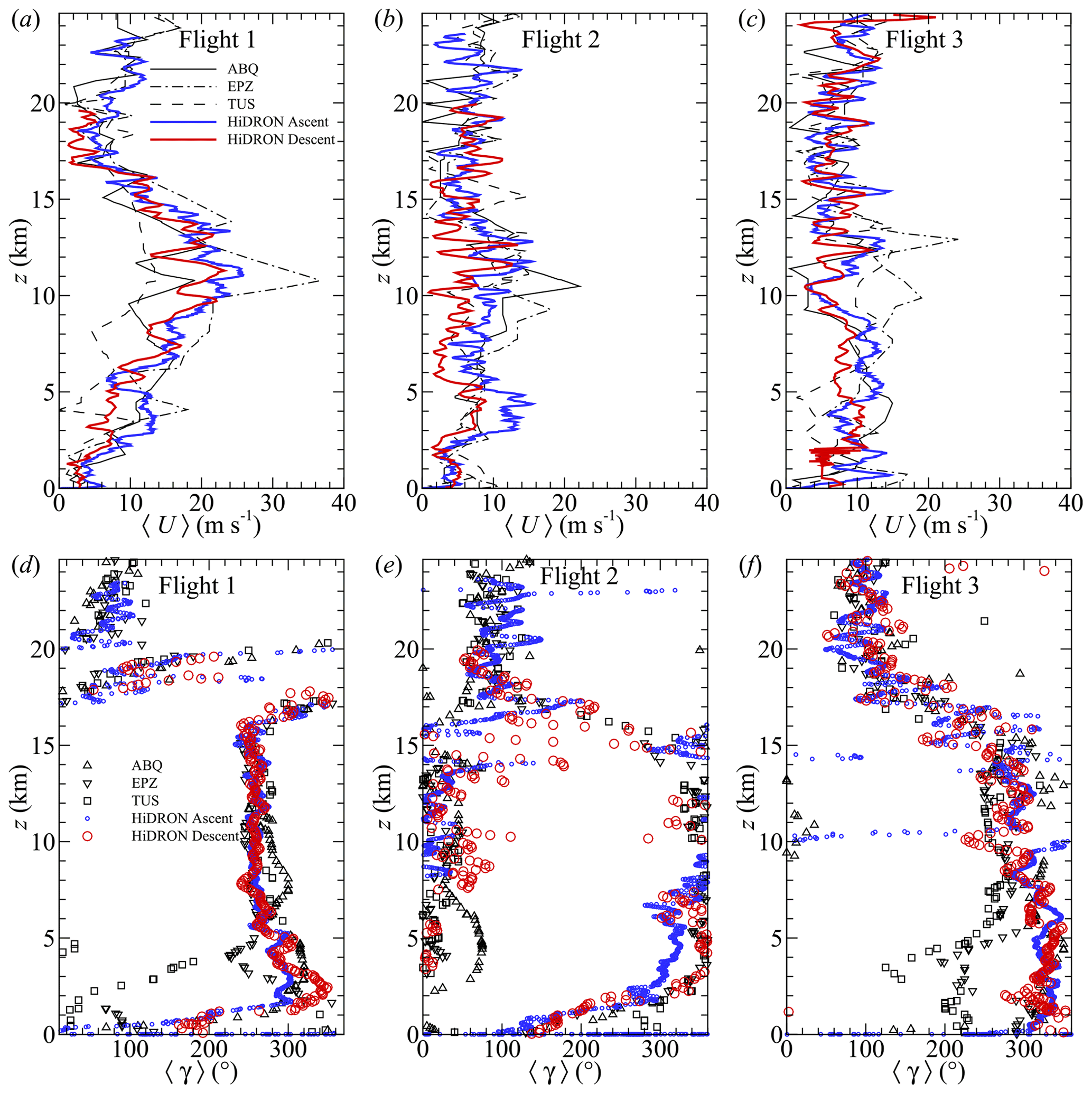
Figure 10Horizontal wind magnitude measured during (a) Flight 1, (b) Flight 2, and (c) Flight 3 compared to NWS radiosonde soundings from the Albuquerque (ABQ), El Paso (EPZ), and Tucson (TUS) forecast offices. Corresponding wind directions are shown for (d) Flight 1, (e) Flight 2, and (f) Flight 3.
In general, the wind magnitude and direction measured by the HiDRON H2 are within the bounds provided by the radiosonde soundings, with the wind direction measured during descent producing good agreement with that reported by the radiosondes and by the GPS on ascent. To assess the agreement with respect to the wind magnitude, we computed the average of the three NWS radiosonde profiles at each altitude recorded by the HiDRON H2. Subsequently, we determined the difference in U at each altitude. The resulting median of the absolute values of these differences was 1.9, 3.4, and 2.3 m s−1 for flights 1, 2, and 3, respectively. Similarly, comparing U measured during ascent and descent by HiDRON H2 yielded median absolute difference values of 2.4, 3.0, and 2.7 m s−1 for flights 1, 2, and 3, respectively.
With respect to the wind magnitude profile itself, the HiDRON measurements do contain short-wavelength (e.g., < 1 km) fluctuations that were evident in both the ascent (GPS ground velocity) and descent (five-hole-probe) wind velocity measurements made using the HiDRON H2. One significant difference between the ascent and descent measurements is the stronger long-wavelength fluctuations (on the order of 2.5 km) measured during descent than those measured during ascent for Flight 1 in the range of 7.5 < z < 12.5 km and for Flight 2 in the range of 11 < z < 13 km. These low-frequency waves are close to that of the orbit pitch at these altitudes (varying from 2 to 3 km) and may, therefore, reflect bias in the wind estimate introduced by the orbital path. However, the magnitude of the differences exceeds the anticipated uncertainty bounds presented in Fig. 5. Furthermore, as discussed in Sect. 2.3, such periodic bias tends to be produced by error in yaw angle, which propagates through the transformation from the body-fixed to the inertial coordinate system. However, this yaw error influences u and v with phase and, therefore, also tends to appear in the wind direction as well (as shown in, e.g., Al-Ghussain and Bailey, 2021). As shown in Fig. 10d for Flight 1, the 〈γ〉 estimates have close correspondence to the 〈γ〉 measured during ascent in the range of 7.5 < z < 12.5 km. It is also possible that the long-wavelength fluctuations in 〈U〉 may be evidence of horizontal heterogeneity in the wind magnitude at these altitudes, although this cannot be determined from the current measurements. Some periodicity in 〈γ〉 is evident during flights 2 and 3 that is not measured during ascent, for example, between 5 and 10 km in the Flight-2 〈γ〉 profiles. However, at these altitudes, no corresponding periodicity is evident in 〈U〉, and the wavelength of the periodicity is shorter than the pitch of the helical flight path; therefore, these oscillations are not believed to be due to bias introduced by the flight path. More detailed quantification of long-wavelength motions is provided through wavelet analysis presented in Sect. 3.2.
Finally, differences in the wind magnitude on the order of 5 m s−1 were observed between measurements made during ascent and descent in the troposphere during flights 2 and 3. It is not clear what the source of this difference is, although there was a time difference of 2 to 4 h between when the aircraft ascended through this region on its balloon and when it descended through the same region in a glide.
To summarize the observations of mean quantities provided in Figs. 9 and 10, atmospheric conditions were similar for flights 2 and 3, which differed from Flight 1. The strongest winds occurred during Flight 1, which had an environmental lapse rate of 8.4 °C km−1 (Fig. 9a) and winds coming from 270°, increasing with altitude to a peak value over 20 m s−1 just above the tropopause (z = 12.5 km), after which the magnitude decreased with increasing z to the stratospheric inversion near z=17 km. This pattern of constant wind direction and high wind magnitude is consistent with the presence of a jet stream, and the NOAA upper-air wind meteorological maps (e.g., as provided in Appendix B) indicate that a tropical jet stream was centered to the southeast of the flight location, over central Texas, during Flight 1, such that the flight path was on the outer edge of the jet. The relative position of the jet stream for Flight 1 also explains the higher wind magnitudes measured at EPZ, which was closer to the center of the jet. Above the jet stream for Flight 1, the winds increase with altitude again, with a significant directional shift indicating that horizontal shear was present above the temperature inversion.
The jet stream had moved to the east by the time of flights 2 and 3 (as shown in Appendix B), which is reflected in the reduced wind magnitude measured during these flights (panels b and e and panels c and f in Fig. 10, respectively), typically below 〈U〉 = 10 m s−1. Wind direction was consistently from the north for z < 15 km for Flight 2, with directional shear observed between z = 15 km and z = 20 km. An environmental lapse rate of 7.9 °C km−1 was measured for Flight 2, whereas a corresponding value of 8.2 °C km−1 was measured for Flight 3. Wind observations during Flight 3 can be summarized as being nearly constant values of 〈U〉≈ 10 m s−1 up to z = 30 km, with winds coming from 300° in the troposphere and changing with altitude to be from 100° at z = 20 km.
3.2 Turbulent quantities
The HiDRON H2 measurements can be used to quantify the intensity of turbulence at different altitudes. For example, through the turbulent kinetic energy, 〈k〉, which was calculated for each statistical segment using the following expression:
Note that, as u(t), v(t), and w(t) were oversampled, an additional filtering step was taken to minimize the influence of high-frequency noise on 〈u′2〉, 〈v′2〉, and 〈w′2〉. To do this, these quantities were calculated by integrating the corresponding velocity spectrum, Fuu(f), Fvv(f), and Fww(f) (equivalent to the one-sided autospectral density function of the detrended velocity component, following the terminology of Bendat and Piersol, 2010). The velocity spectra were found for each statistical segment using Welch's periodogram method implemented with a variance-preserving Hanning window, three subintervals, and a 50 % overlap, implemented using the “pwelch” MATLAB function. The final low-pass-filtered estimates of 〈u′2〉, 〈v′2〉, and 〈w′2〉 were then determined by integrating Fuu(f), Fvv(f), and Fww(f) over the frequency range in which they were above the noise floor. The upper limit of this range was determined by identifying the frequency at which noise began to dominate the integration over velocity fluctuations, leading to an increase in Fuu, Fvv, or Fww with rising f. The procedure employed for this process was to visualize the spectra in a “compensated” form, whereby fFuu is plotted on semilogarithmic axes as a function of f. Such compensated, or “pre-multiplied,” spectra facilitate the visualization of energy spectra when viewed in this manner, as they allow for a clearer representation of the frequency dependence of the relative contribution of each frequency to the overall energy content. This is because, for example,
Hence when fFd(log f) begins to increase on a semilogarithmic plot at high frequencies, this indicates a frequency range in which the energy content increases with f. Given that universal equilibrium range turbulence will decrease with respect to the energy content with f, the minimum in fFd(log f) indicates a frequency at which the noise begins to have a greater contribution to the variance than the turbulence content.
The upper bound identified using this approach was consistent with the probe's maximum frequency response in the boundary layer and varied between 1 and 20 Hz above the boundary layer, with the higher upper frequency bounds corresponding to instances in which there was an increased low-frequency content in Fuu, Fvv, or Fww. It is worth noting that the Reynolds stresses filtered in this manner were observed to be an average of 85 % of the variance of the corresponding unfiltered signal, reflecting the influence of high-frequency noise on statistics.
Due to the time averaging used, the value of 〈k〉 will only incorporate contributions from relatively short wavelengths, corresponding to the distance traveled by the aircraft during the averaging time. Thus, an additional metric that can be used to quantify turbulence is the turbulent kinetic energy dissipation rate (ε). Within equilibrium homogeneous turbulence, ε can be expected to scale with the rate of production of k; within the inertial subrange, it should scale with k and the wavenumber range of the inertial subrange. The dissipation rate is particularly useful for turbulent quantification in atmospheric turbulence for which the scale of the energy-containing eddies may be quite large or ill-defined, as ε can be determined from small-scale fluctuations without requiring resolution of the low-wavenumber turbulence.
As determination of ε using Eq. (2) requires measurement of spatial gradients of velocity over distances on the order of the Kolmogorov scale, it is challenging to directly measure ε in the atmosphere without additional assumptions. Thus, indirect estimates of ε are usually employed. Here, we assume the presence of a sufficiently high Reynolds number for the formation of an inertial subrange in the energy spectrum. Under such conditions, the one-dimensional longitudinal wavenumber velocity spectrum in the inertial subrange is expected to follow a scaling such that
as suggested by Kolmogorov (1941) using the one-dimensional Kolmogorov constant of 0.49 empirically determined by Saddoughi and Veeravalli (1994). κℓ is the longitudinal wavenumber and the wavenumber velocity spectrum calculated using the velocity component parallel to κℓ.
To determine 〈ε〉 within each statistical segment, Eℓℓ(κℓ) was estimated using the component of the wind velocity aligned with −VR. This was calculated by first rotating the coordinate system from the east–north–up alignment to instead align u with an axis parallel to the velocity of the aircraft within the air, i.e., we define uℓ(t) as the component of the wind velocity vector found by projection of the wind velocity vector, U, in the direction formed by 〈−VR〉. The velocity spectrum of uℓ(t) in the frequency domain, Fℓℓ(f), was then calculated on the rotated wind velocity vector following the same procedure used to calculate the Reynolds stresses. We note that, as Eq. (14) is defined in the wavenumber domain, Fℓℓ(f) was then transformed to Eℓℓ(κℓ). To do this, the longitudinal wavenumber, κℓ, was approximated using Taylor's frozen-flow hypothesis such that . We then found the longitudinal velocity spectrum in the wavenumber domain using , where this last operation was conducted to ensure that
Finally, Eq. (14) was used to estimate 〈ε〉 with a least-squares fit to Eℓℓ. This fit was conducted over the κℓ range corresponding to the frequency range used in the calculation of 〈k〉. The result is an estimate of ε for each statistical segment, i.e., 〈ε〉. Note that the approach used here provides only an approximation of 〈ε〉, as Eℓℓ(κℓ) will only follow Eq. (14) in the presence of inertial turbulence, whereas the fit will always provide a nonzero value of 〈ε〉, even if no turbulence is present. Therefore, some caution is required when interpreting these values.
The values of 〈k〉 are compared to the corresponding values of 〈ε〉 in Fig. 11. Although there is significant scatter, the general trend follows the expected for this calculation approach, demonstrating some intrinsic consistency in the different calculations. Additionally, it is important to note that, alongside the implicit assumptions inherent in calculating 〈ε〉, the method employed to compute 〈k〉 only incorporates the energy content corresponding to wavelengths smaller than the statistical segment length (or frequencies higher than the inverse of the time taken to traverse that segment length).
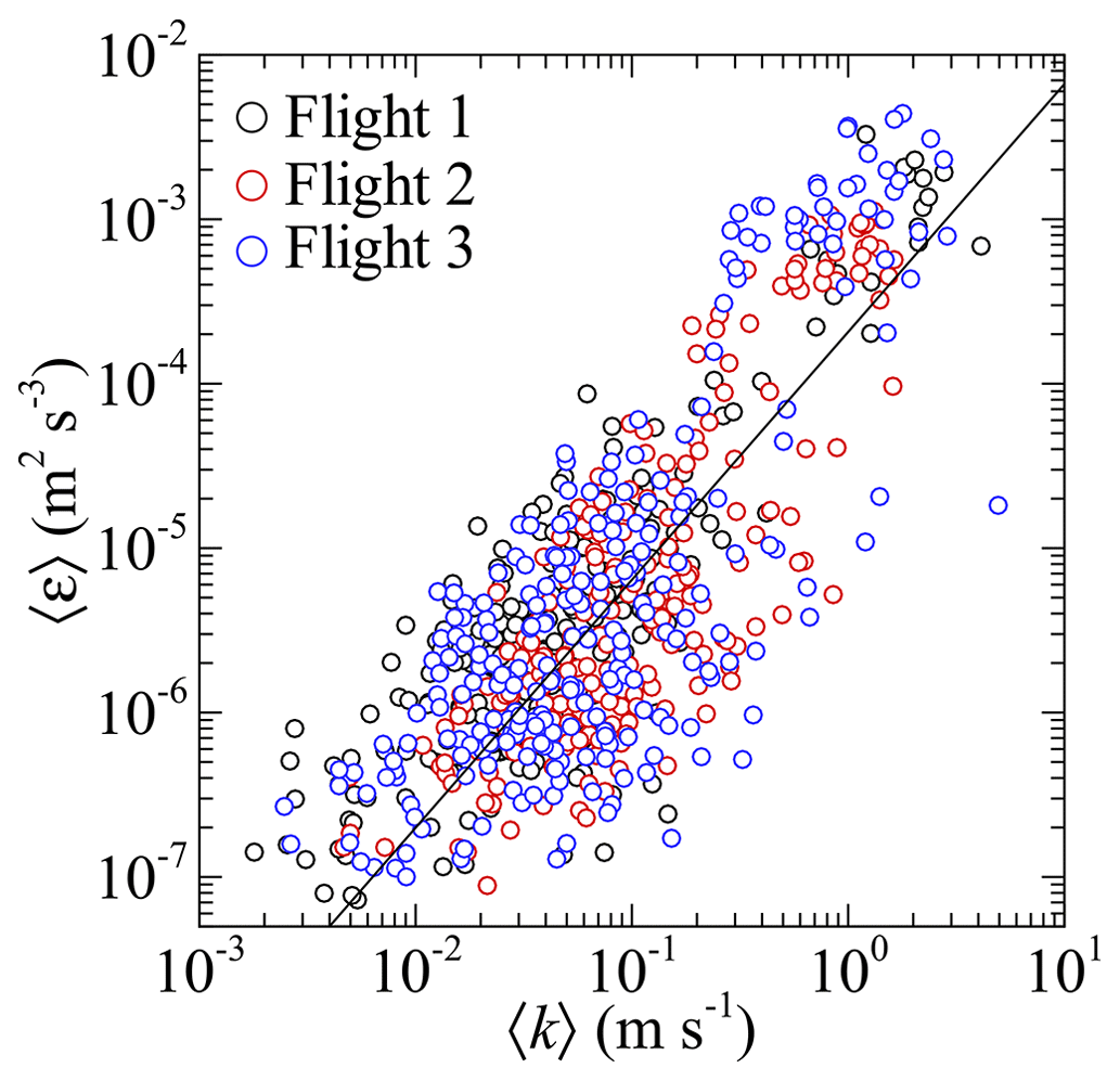
Figure 11Comparison of the turbulent kinetic energy and turbulent kinetic energy dissipation rate calculated within each statistical segment. The solid line indicates the slope.
The corresponding statistic of the eddy dissipation rate, , is often used in the aviation industry to quantify turbulence. Following Huang et al. (2019), this metric allows the turbulence to be characterized as follows: steady for EDR<0.1, weak for EDR between 0.1 and 0.3, moderate for EDR between 0.3 and 0.5, strong for EDR between 0.5 and 0.8, and very strong for EDR>0.8. The measured profiles of 〈k〉 and 〈EDR〉2 are compared to each other for all three flights in Fig. 12a, c, and e. For all flights, the 〈EDR〉 values indicate that only weak turbulence was present. The most noticeable region of turbulence is just above and within the boundary layer, evident in Fig. 12a as an increase in 〈k〉 and 〈EDR〉2 for z < 2 km, with slightly thicker regions of elevated 〈k〉 evident in Fig. 12b and c over the range of z < 4 km and z < 3 km for flights 2 and 3, respectively.
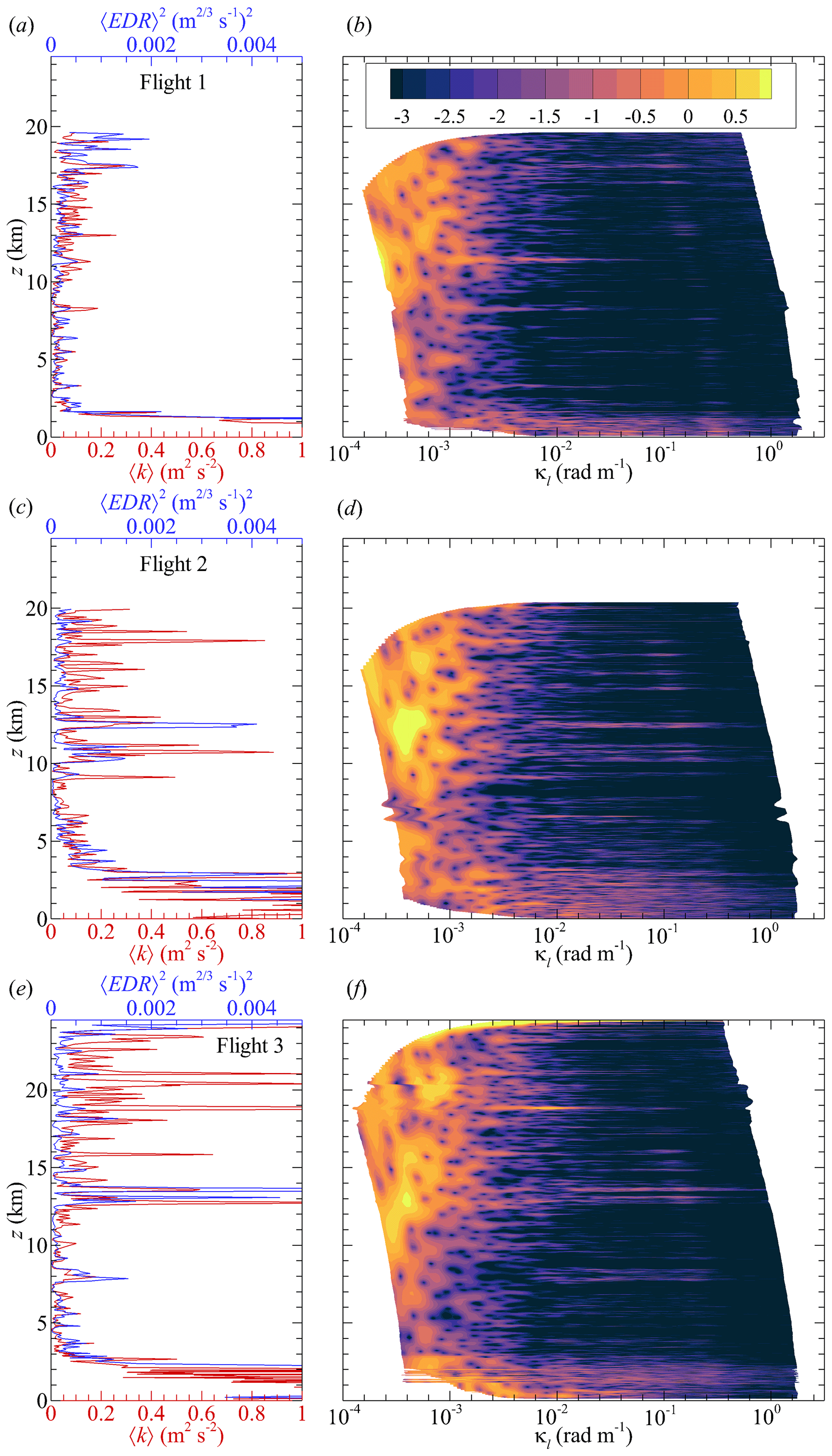
Figure 12Profiles of 〈k〉 and 〈EDR〉2 for (a) Flight 1, (c) Flight 2, and (e) Flight 3. Contours of are also shown for (b) Flight 1, (d) Flight 2, and (f) Flight 3 as functions of κℓ and z. Contour levels are the same in panels (b), (d), and (f).
Above the boundary layer turbulence, 〈k〉 and 〈EDR〉2 are largely in agreement, although there are numerous localized regions where elevated 〈k〉 values were measured for stratospheric altitudes during flights 2 and 3. To investigate these regions further, we employ the continuous wavelet transform, an approach often used in time–frequency analysis due to its ability to discriminate frequency content within a signal as a function of time. Here, we employ the wavelet transform to examine the energy content of the measured velocity signal due to the presence of both low-frequency and high-frequency motions, which, as observed in Fig. 8, vary with altitude and, consequently, with time. Wavelet transforms eliminate the need for segmenting the time series, as required for calculating Fℓℓ(f), thereby avoiding potential bias introduced by the selection of segment length. Thus, we chose to leverage the wavelet transform's capability to discern the time (and hence altitude) dependence of the frequency content of uℓ(t).
The continuous wavelet transform is defined through convolution of the time-dependent signal, here uℓ(t), with a wavelet function, Ψ, such that
where Ψ∗ is the complex conjugate of the selected wavelet function, a is the scale parameter, and b is the position parameter. The result of the transform is the wavelet coefficient, W, as a function of a and b which can be related to f and t, respectively (see, e.g., Tavoularis, 2024). Therefore, the wavelet coefficient is a complex-valued result whose amplitude reflects the frequency-dependent amplitude of Ψ providing the best agreement with the original signal at each point in its time series. In this implementation, we utilized the analytical Morlet wavelet in MATLAB over a frequency range from 0.001 to 5 Hz. These frequencies correspond to approximately the rate at which orbits were completed and half the maximum frequency response of the probe under low-pressure and low-temperature conditions, respectively. The Morlet wavelet is a complex harmonic function modulated by a Gaussian envelope and provides a measure of the frequency content of a signal over a short time interval ∼ s long.
Figure 12b, d, and f present the wavelet transform of uℓ(t) for flights 1, 2, and 3, respectively, as logarithmically scaled isocontours of the complex modulus of the wavelet coefficient squared, , which is referred to as the wavelet power spectrum. To transform the results from the time–frequency domain to the spatial domain, the plot is presented as a function of z (which is time dependent) and . Note that the scale of Ψ which can be convoluted with uℓ(t) is limited by the length of the available signal in time at the start and end of the time series; hence, the low-frequency boundary of the wavelet power spectrum shown in Fig. 12b, d, and f is time dependent.
Noticeable in Fig. 12b, d, and f is the significant long-wavelength content for κℓ<0.003 (wavelengths larger than 2 km), with the highest coefficient values measured during flights 2 and 3 when z > 10 km. This long-wavelength content is the signature of the long-period fluctuations in Fig. 8 and fluctuations with altitude measured in Fig. 10. High-frequency content is also evident, not only in the proximity of the boundary layer but also in thin regions corresponding to altitudes at which elevated 〈k〉 and 〈EDR〉 are observed in Fig. 12a, c, and e. For example, for Flight 1, distinct regions of elevated appear for κℓ<0.1 at z ≈ 8 km and z ≈ 12 km and with higher-wavenumber content around z ≈ 17 km. It can be observed that 〈EDR〉2 and 〈k〉 have the greatest agreement when uℓ contains high-wavenumber content, i.e., when an inertial subrange is present (as implied by the approach used to determine 〈ε〉). Conversely when 〈k〉 is much larger than 〈EDR〉2, specifically the larger spikes in 〈k〉 measured during flights 2 and 3 above z = 10 km, it can be observed that these events correspond to instances in which uℓ has energy content at low wavenumbers. Hence, the elevated 〈k〉 for z > 15 km in Fig. 12c and e appears to be due to low-wavenumber energetic contributions to 〈k〉 and the 〈EDR〉 calculation approach used here is unable to capture these low-wavenumber contributions.
3.3 Infrasonic detection of turbulence
Before we can explore the connection between the infrasonic sound energy detected by the microphone and the turbulent kinetic energy measured by the five-hole probe, we need to quantify the measured infrasound energy. To do this, we use the variance of the pressure fluctuations in the acoustic signal measured by the microphone, σ2. We note that σ2 will include pressure waves generated by the long-wavelength fluctuations shown in Fig. 12b, d, and f (which indicate significant energy content in the velocity fluctuations at wavenumbers below 0.003) in addition to any inertial turbulence that may be present at higher frequencies. To capture this long-wavelength motion and corresponding low-frequency acoustic waves, we expand our segment length to 240 s (corresponding to the nominal time it took the HiDRON H2 to complete half an orbit) in order to ensure that the low-frequency content is included in the variance calculation for both the infrasound and wind velocity fluctuations. Statistical averages calculated over this longer segment size are indicated using square brackets, [ ]. Profiles of [σ2] measured during all three flights are presented in Fig. 13a, b, and c.
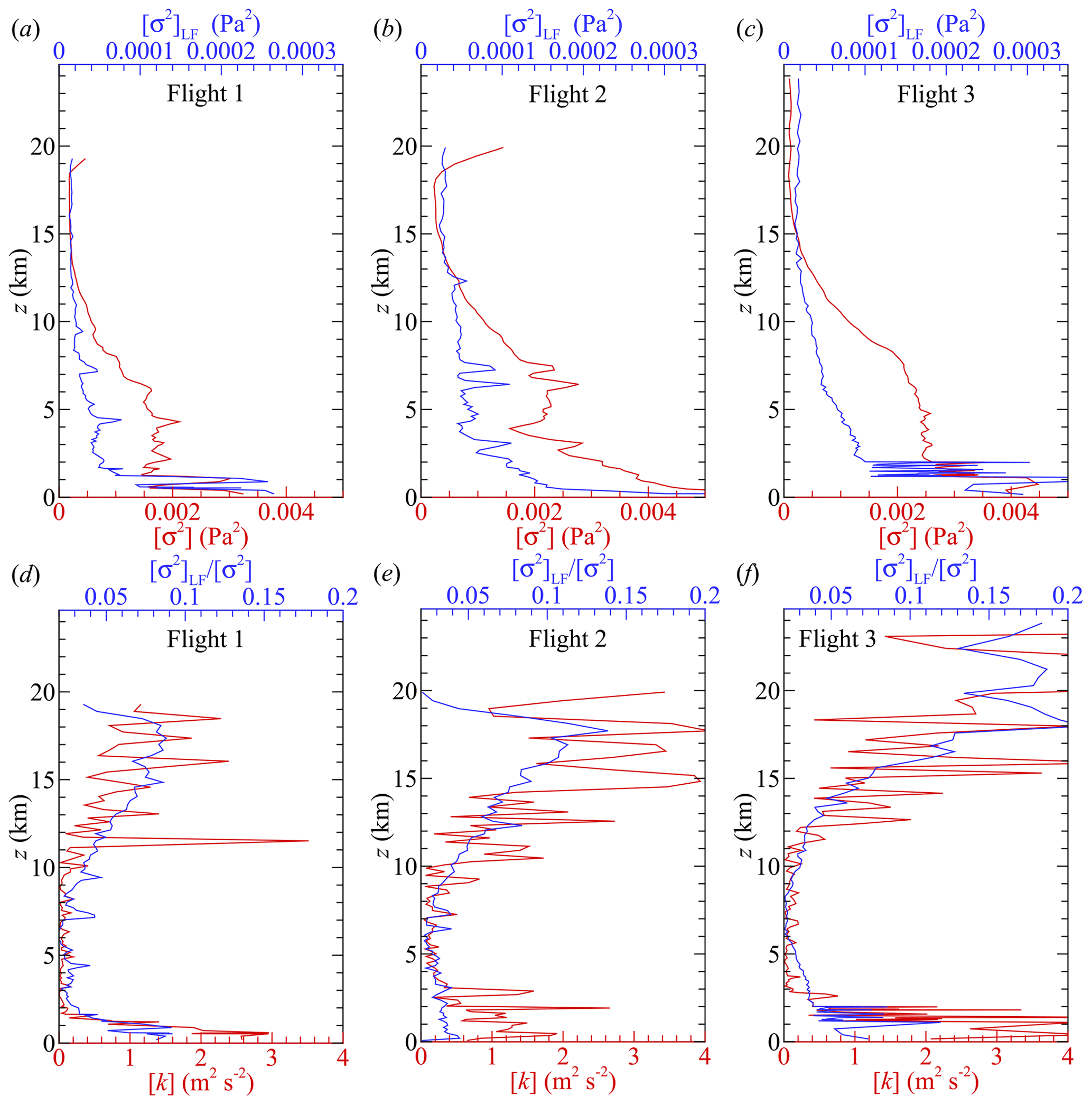
Figure 13Infrasonic microphone signal as measured through its variance ([σ2]) compared to variance of the low-pass-filtered signal at 20 Hz ([σ2]LF) for (a) Flight 1, (b) Flight 2, and (c) Flight 3. The ratio compared to turbulent kinetic energy ( [k]) for (d) Flight 1, (e) Flight 2, and (f) Flight 3.
Noticeably, there was a decrease in signal amplitude measured with increasing altitude for all three flights. It was found that this decrease closely corresponds to the reduction in local atmospheric pressure; therefore, it is attributed to increased atmospheric absorption due to the increase in the molecular mean free path with altitude (Bass et al., 2007). Despite this altitude dependence, localized increases in [σ2] were observed, particularly near the boundary layer. When we isolate only the infrasonic part of the acoustic amplitude by integrating the power spectrum of the microphone signal over the frequency range below 20 Hz, which we refer to as [σ2]LF, we observe a similar but unequal attenuation, as also depicted in Fig. 13a, b, and c.
Any altitude-dependent attenuation resulting from the decrease in the molecular mean free path will be contingent on both local temperature and pressure and apply uniformly across the bandwidth of the microphone. Therefore, the ratio , which indicates the proportion of the total microphone energy measured within the infrasonic range, can serve to adjust for signal absorption with altitude, assuming consistent frequency response characteristics of the microphone across different altitudes. This ratio is compared to [k] in Fig. 13d, e, and f, with [k] selected for this comparison over 〈k〉 due to its inclusion of the long-wavelength turbulent kinetic energy content shown in Fig. 12d, e, and f. When analyzed in this manner, the resulting profile of infrasonic amplitude shows a pronounced correspondence to the [k] profile. Consequently, it appears that the infrasonic microphone is particularly sensitive to the long wavelengths detected in the stratosphere and, to a lesser extent, those in the vicinity of the boundary layer. However, the profile appears as a filtered version of the [k] profile.
Because the infrasonic microphone registers pressure waves that have traveled an unknown distance from their origin, whereas the five-hole probe can only measure the velocity fluctuations in situ, we should not anticipate a precise correlation between and [k]. Moreover, the omnidirectional propagation of sound adds complexity, implying that the microphone may pick up sound from sources not measured by the five-hole probe. Hence, these results can only provide qualitative support with respect to the ability of the microphone to detect atmospheric turbulence, as a quantitative analysis would also require information about the distance and strength of the source of infrasonic energy.
It is worth noting that the normalization of employed here does not capture the rise in [k] observed near the boundary layer. This is due to the increase in [σ] caused by the heightened broadband turbulent activity in the boundary layer. Consequently, the ratio remains relatively constant across the boundary layer. However, Fig. 13a, b, and c demonstrate that there is a rise in within the boundary layer, aligning with the increase in [k]. This observation is consistent with the ground-based findings of Cuxart et al. (2015).
3.4 Stability conditions
Profiles of the square Brunt–Väisälä frequency (N2) and square shear frequency (S2) provide some perspective on the altitude dependence of static stability and horizontal velocity shear (and hence the potential for turbulence generation). However, approximating the mean vertical gradients of wind and virtual potential temperature required to calculate N2 and S2 using Eqs. (5) and (6) becomes somewhat ambiguous for the HiDRON H2 measurements. This is due to the shallow glide slope of the particular helical flight path flown in these experiments, which introduces an increased sensitivity to horizontal gradients of U and θv compared with that of the vertical gradients.
Therefore, different approaches were attempted to calculate N2 and S2. For the initial approach that we present here, we assume horizontal homogeneity and attempt to replicate the expected response of a radiosonde to changes in the vertical wind structure, . To do so, we assume a radiosonde time response for wind on the order of 40 s (Dirksen et al., 2014), which is introduced in commercial radiosondes by filtering of the pendulum effects and GPS noise as well as by the inertia of the balloon itself (Scoggins, 1965). This time response, when combined with a typical rise rate of 5 m s−1, equates to a vertical resolution of approximately 200 m. Therefore, prior to calculating the vertical gradients, u(t) and v(t) were filtered using a moving average over a time span equivalent to a change in z of 200 m. Then, to enable calculation of gradients in the vertical direction over Δz = 100 m intervals (the approximate turbulent layer thickness estimated by Ko et al., 2019), the wind components u(t), v(t), and θv(t) were then averaged over Δz = 100 m bins, allowing the calculation of the vertical gradients using the resulting bin-averaged values separated by Δz = 100 m. However, these gradient values were no longer at the same z location as the location where 〈θv〉 values were calculated. Therefore, prior to calculating N2 and S2, the gradients calculated at a resolution of Δz = 100 m had to be interpolated to the z location corresponding to each statistical segment.
The square Brunt–Väisälä frequency and square shear frequency calculated this way are presented as solid lines in Fig. 14 for each flight. The results show large oscillations with altitude for all three flights, particularly in S2, which can be expected from Fig. 10. However, when is compared to both 〈k〉 and 〈EDR〉, as done in Fig. 15a and b, respectively, the resulting trend is generally consistent with the expected behavior of increased turbulence intensity at low Ri. Specifically, the high-turbulence-intensity events (independent of whether quantified through 〈k〉, as done in Fig. 15a, or 〈EDR〉, as done in Fig. 15b) largely occur when Ri<1, although there are some instances of elevated turbulence when Ri>1 and instances where no turbulence is evident when Ri<1.
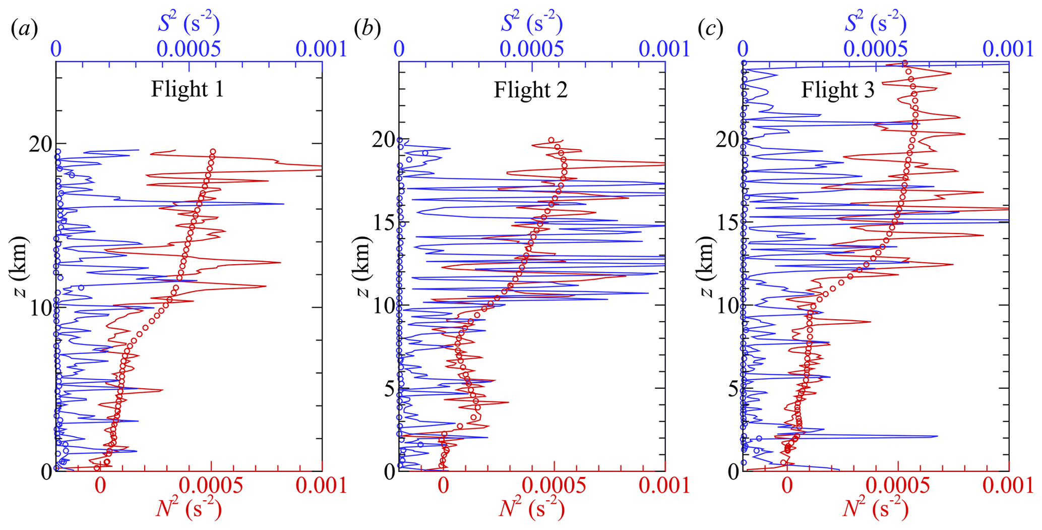
Figure 14The square Brunt–Väisälä frequency (N2) and square shear frequency (S2) profiles for (a) Flight 1, (b) Flight 2, and (c) Flight 3. Solid lines show profiles calculated using vertical gradients calculated along flight trajectory, whereas symbols show profiles calculated using vertical gradients calculated between neighboring orbits at same azimuthal position.
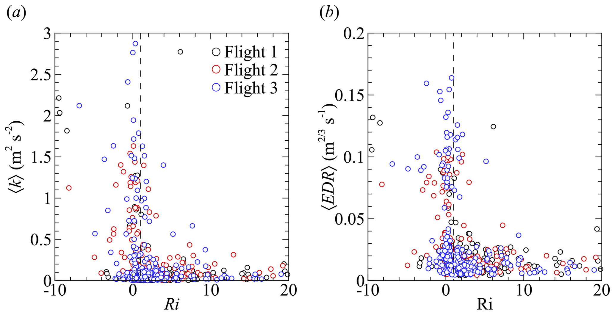
Figure 15Comparison of (a) turbulent kinetic energy (〈k〉) and (b) eddy dissipation rate (〈EDR〉) to gradient Richardson number (Ri) calculated along flight trajectory. The dashed vertical line indicates Ri=1.
As the helical descent of the aircraft results in approximately 1500 m of horizontal travel for every 100 m of decent, horizontal variability in the measured variables have an outsized impact on the calculation of Ri. In an attempt to eliminate the required assumption of horizontal homogeneity for the calculation of Ri, an alternative approach was attempted to calculate vertical gradients, whereby the vertical profiles were expanded along the circumference of the aircraft's orbit. For each statistical segment, the two nearest segments in the z direction were used to calculate the vertical gradients using central differencing. In this way, the gradients were calculated vertically across individual orbits, rather than along the helical path. However, this results in a gradient calculation with a vertical scale of the same order as the pitch of the helix, which was approximately 2.5 km and, therefore, much larger than the thickness of the layers of turbulence observed in Fig. 12.
The values of S2 and N2 calculated this way are shown using symbols in Fig. 14a, b, and c. This calculation approach effectively reproduces the trend in the N2 vertical profiles calculated along the flight path but contains fewer fluctuations, particularly for z > 10 km. The corresponding S2 profiles, however, were an order of magnitude smaller when calculated across the orbits than when calculated along the flight path (reflected in the values near zero in Fig. 14a, b, and c) and, therefore, resulted in Ri values on the order of 103. The lower values of S2 when calculated between the orbits likely reflect the larger vertical distances involved in the differencing across the orbits which will effectively filter out many of the vertical wind gradients shown in Fig. 10a, b, and c. This approach is presented here, as it may be more successful for flight trajectories with a smaller orbit diameter and a smaller vertical pitch between orbits.
This report describes a balloon-launched glider UAS and instrumentation intended for measuring the statistical structure of atmospheric turbulence. To conduct these quantitative measurements, the aircraft was equipped with a five-hole probe for measuring the three-component wind vector and with pressure, temperature, and humidity sensors integrated into the aircraft.
These instruments allowed the measurement of vertical profiles of T, RH, U, and γ up to z = 25 . These profiles compared favorably with the nearest publicly available National Weather Service (NWS) radiosonde data for T and RH, although there were some noticeable differences in the RH values, which were lower than the radiosonde values for z > 7 km. There were also indications that additional corrections may be needed to T within the stratosphere. Wind profiles had a median difference on the order of 2.5 m s−1 with the available NWS radiosonde profiles and the GPS-derived wind velocity measured during ascent.
The descent trajectory allowed for the calculation of 〈k〉 and 〈ε〉 over a large horizontal distance relative to the vertical distance traveled. The resulting vertical profiles suggest that isolated regions of weak turbulence were present in all three flights; moreover, by examining the wavelet transform of the longitudinal velocity, it was observed that these isolated regions could have a different wavelength content depending on altitude. The wavelet transforms also indicated that long-wavelength fluctuations provided a significant contribution to the energy content for z > 10 km. The onboard infrasonic microphone captured these long-wavelength fluctuations as low-frequency acoustic energy. As the UAS approached the boundary layer, the microphone also detected a rise in broadband acoustic energy, consistent with the broader frequency content of turbulence within this layer measured by the five-hole probe. While these findings are qualitative, they imply that the infrasonic microphone is responsive to long-wavelength turbulent kinetic energy. Future research aims to establish a more quantitative relationship, necessitating additional information about the distance of the sensor from the source of turbulent kinetic energy as well as information about the turbulence strength at the source.
An attempt was also made to calculate the gradient Richardson number from the temperature and wind profiles; however, the helical flight trajectory of the UAS introduces ambiguity in the time and length scales used for determining the mean vertical gradients. A method was proposed which smoothed the wind velocity prior to calculating the gradients across 100 m vertical increments. This resulted in gradient Richardson numbers that corresponded to enhanced 〈k〉 and 〈ε〉 when Ri<1, but there were outliers, which suggested improvements could be made to the calculation approach. An alternative approach was presented which calculated the vertical gradients across the pitch of the helical flight path. This produced similar results for N2, but the S2 results were an order of magnitude smaller due to the pitch being on the order of 2.5 km. The result was very high Ri values that predicted stable conditions, even when turbulence was present.
Despite this ambiguity, these initial flights suggest that potential exists for this measurement approach to be used for high-altitude turbulence research, for example, enabling detailed analysis of length scales and anisotropy of turbulence. However, additional flights would be beneficial to assess the capabilities of this measurement technique. For example, for the three flights considered here, the turbulence above the boundary layer was relatively weak and limited in occurrence. Measurements under more unstable conditions would lead to increased opportunities to conduct turbulence observations. Furthermore, flight patterns could be designed to allow the examination of potential inhomogeneity of the statistics, for example, by taking advantage of the helical trajectory taken by the glider during its descent to produce depictions of the horizontal heterogeneity of measured statistics. Additional flight patterns could also be designed with a tighter helical descent to better calculate the gradient Richardson number, with higher vertical resolution. Finally, improvements could be made to the data acquisition system that would lessen the signal-to-noise ratio of the acquisition system, simplifying post-processing of the measurements and providing higher resolution of instances of turbulence encountered.
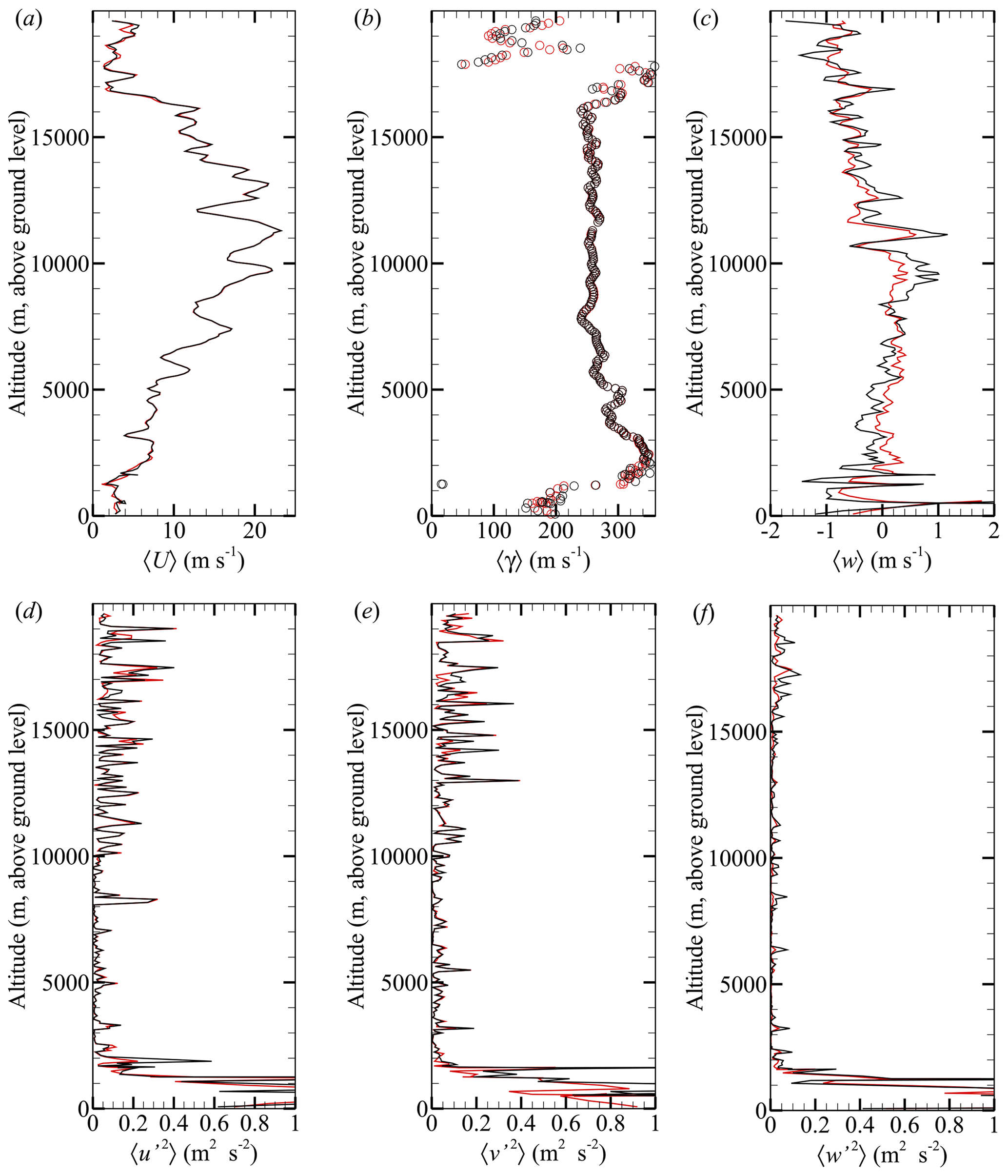
Figure A1Comparison of the (a) horizontal wind velocity magnitude, (b) horizontal wind direction, and (c) vertical component of wind velocity calculated using the ΔP1, ΔP32, and ΔP54 transducers to find Q, α, and β (shown in red) with the same properties calculated using only the ΔP1 and ΔP32 transducers to calculate Q and β with α determined from the aircraft angle of attack measurement (shown in black). Comparison of the resulting (d) 〈u′2〉, (e) 〈v′2〉, and (f) 〈w′2〉 Reynolds stress tensor components are also shown.
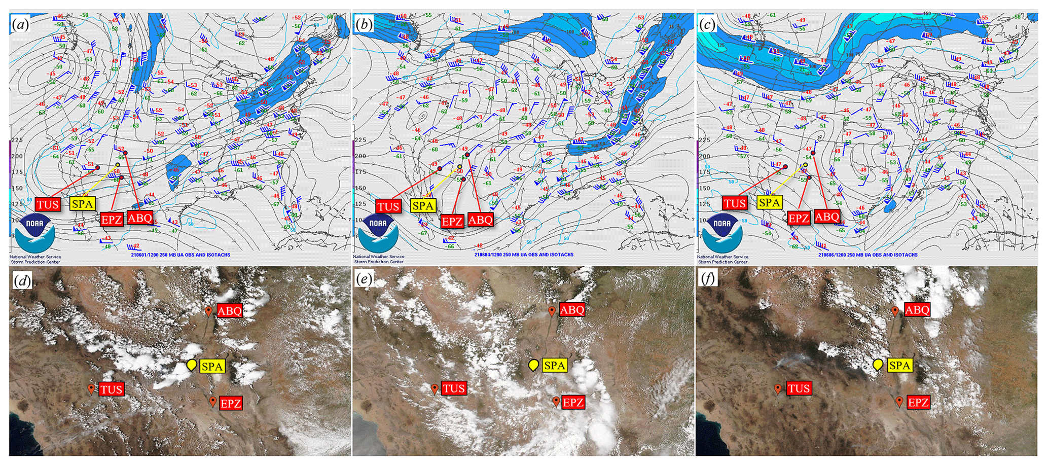
Figure B1NOAA jet stream maps at 250 mbar (10.366 km) for (a) Flight 1, (b) Flight 2, (c) Flight 3 and satellite images of cloud cover (, ) for (d) Flight 1, (e) Flight 2, and (f) Flight 3. Red pins indicate the NWS sounding sites, whereas the yellow pin indicates the measurement location at Spaceport America (SPA).
Data from these flights are available from the corresponding author upon request.
A video compilation of the aircraft preparation, flight, and recovery is available at https://vimeo.com/568101900 (login may be required; Craine, 2021).
SCCB, GDP, and NC planned the experiment. SCCB, RDN, GDP, and AS carried out the experiment. Data analysis was conducted by ANH and SCCB, who also prepared the initial draft of the manuscript with input from the remaining authors.
The contact author has declared that none of the authors has any competing interests.
Publisher's note: Copernicus Publications remains neutral with regard to jurisdictional claims made in the text, published maps, institutional affiliations, or any other geographical representation in this paper. While Copernicus Publications makes every effort to include appropriate place names, the final responsibility lies with the authors.
The authors would like to dedicate this work to Qamar Shams, who worked at NASA Langley Research Center and graciously assisted with the implementation and the loan of the infrasonic microphone from NASA.
This research has been supported by the National Aeronautics and Space Administration, Space Technology Mission Directorate (grant no. 80NSSC20K0102).
This paper was edited by Jorge Luis Chau and reviewed by four anonymous referees.
Abarbanel, H. D. I., Holm, D. D., Marsden, J. E., and Ratiu, T.: Richardson Number Criterion for the Nonlinear Stability of Three-Dimensional Stratified Flow, Phys. Rev. Lett., 52, 2352–2355, https://doi.org/10.1103/PhysRevLett.52.2352, 1984. a
Al-Ghussain, L. and Bailey, S. C. C.: An approach to minimize aircraft motion bias in multi-hole probe wind measurements made by small unmanned aerial systems, Atmos. Meas. Tech., 14, 173–184, https://doi.org/10.5194/amt-14-173-2021, 2021. a, b
Al-Ghussain, L. and Bailey, S. C. C.: Uncrewed Aircraft System Measurements of Atmospheric Surface-Layer Structure During Morning Transition, Bound.-Lay. Meteorol., 185, 229–258, https://doi.org/10.1007/s10546-022-00729-2, 2022. a, b
Alisse, J.-R., Haynes, P. H., Vanneste, J., and Sidi, C.: Quantification of stratospheric mixing from turbulence microstructure measurements, Geophys. Res. Lett., 27, 2621–2624, https://doi.org/10.1029/2000GL011386, 2000. a
Bailey, S. C. C., Canter, C. A., Sama, M. P., Houston, A. L., and Smith, S. W.: Unmanned aerial vehicles reveal the impact of a total solar eclipse on the atmospheric surface layer, P. Roy. Soc. A-Math. Phy., 475, 20190212, https://doi.org/10.1098/rspa.2019.0212, 2019. a, b
Bailey, S. C. C., Sama, M. P., Canter, C. A., Pampolini, L. F., Lippay, Z. S., Schuyler, T. J., Hamilton, J. D., MacPhee, S. B., Rowe, I. S., Sanders, C. D., Smith, V. G., Vezzi, C. N., Wight, H. M., Hoagg, J. B., Guzman, M. I., and Smith, S. W.: University of Kentucky measurements of wind, temperature, pressure and humidity in support of LAPSE-RATE using multisite fixed-wing and rotorcraft unmanned aerial systems, Earth Syst. Sci. Data, 12, 1759–1773, https://doi.org/10.5194/essd-12-1759-2020, 2020. a
Balsley, B. B., Lawrence, D. A., Woodman, R. F., and Fritts, D. C.: Fine-scale characteristics of temperature, wind, and turbulence in the lower atmosphere (0–1,300 m) over the south Peruvian coast, Bound.-Lay. Meteorol., 147, 165–178, 2013. a
Balsley, B. B., Lawrence, D. A., Fritts, D. C., Wang, L., Wan, K., and Werne, J.: Fine Structure, Instabilities, and Turbulence in the Lower Atmosphere: High-Resolution In Situ Slant-Path Measurements with the DataHawk UAV and Comparisons with Numerical Modeling, J. Atmos. Ocean. Tech., 35, 619–642, https://doi.org/10.1175/JTECH-D-16-0037.1, 2018. a
Barat, J. and Bertin, F.: Simultaneous Measurements of Temperature and Velocity Fluctuations Within Clear Air Turbulence Layers. Analysis of the Estimate of Dissipation Rate by Remote Sensing Techniques, J. Atmos. Sci., 41, 1613–1619, https://doi.org/10.1175/1520-0469(1984)041<1613:SMOTAV>2.0.CO;2, 1984. a, b
Barbieri, L., Kral, S. T., Bailey, S. C. C., Frazier, A. E., Jacob, J. D., Reuder, J., Brus, D., Chilson, P. B., Crick, C., Detweiler, C., Doddi, A., Elston, J., Foroutan, H., González-Rocha, J., Greene, B. R., Guzman, M. I., Houston, A. L., Islam, A., Kemppinen, O., Lawrence, D., Pillar-Little, E. A., Ross, S. D., Sama, M. P., Schmale, D. G., Schuyler, T. J., Shankar, A., Smith, S. W., Waugh, S., Dixon, C., Borenstein, S., and de Boer, G.: Intercomparison of Small Unmanned Aircraft System (sUAS) Measurements for Atmospheric Science during the LAPSE-RATE Campaign, Sensors, 19, 2179, https://doi.org/10.3390/s19092179, 2019. a
Bärfuss, K., Pätzold, F., Altstädter, B., Kathe, E., Nowak, S., Bretschneider, L., Bestmann, U., and Lampert, A.: New setup of the UAS ALADINA for measuring boundary layer properties, atmospheric particles and solar radiation, Atmosphere, 9, 28, https://doi.org/10.3390/atmos9010028, 2018. a
Bass, H. E., Hetzer, C. H., and Raspet, R.: On the speed of sound in the atmosphere as a function of altitude and frequency, J. Geophys. Res.-Atmos., 112, D15110, https://doi.org/10.1029/2006JD007806, 2007. a
Bendat, J. S. and Piersol, A. G.: Random Data: Analysis and Measurement Procedures, 3rd edn., Wiley Interscience, New York, USA, https://doi.org/10.1002/9781118032428, 2010. a
Bertin, F., Barat, J., and Wilson, R.: Energy dissipation rates, eddy diffusivity, and the Prandtl number: An in situ experimental approach and its consequences on radar estimate of turbulent parameters, Radio Sci., 32, 791–804, https://doi.org/10.1029/96RS03691, 1997. a
Bohn, D. and Simon, H.: Mehrparametrige Approximation der Eichräume und Eichflächen von Unterschall-bzw. Überschall-5-Loch-Sonden, tm-Tech. Mess., 468, 81–89, 1975. a
Bowman, D. C. and Lees, J. M.: Infrasound in the middle stratosphere measured with a free-flying acoustic array, Geophys. Res. Lett., 42, 10010–10017, https://doi.org/10.1002/2015GL066570, 2015. a
Bowman, H. S. and Bedard, A. J.: Observations of infrasound and subsonic disturbances related to severe weather, Geophys. J. Int., 26, 215–242, 1971. a
Calmer, R., Roberts, G. C., Preissler, J., Sanchez, K. J., Derrien, S., and O'Dowd, C.: Vertical wind velocity measurements using a five-hole probe with remotely piloted aircraft to study aerosol–cloud interactions, Atmos. Meas. Tech., 11, 2583–2599, https://doi.org/10.5194/amt-11-2583-2018, 2018. a
Chunchuzov, I. P., Kulichkov, S. N., Popov, O. E., and Perepelkin, V. G.: Infrasound generation by meteorological fronts and its propagation in the atmosphere, J. Atmos. Sci., 78, 1673–1686, https://doi.org/10.1175/jas-d-20-0253.1, 2021. a
Clayson, C. A. and Kantha, L.: On Turbulence and Mixing in the Free Atmosphere Inferred from High-Resolution Soundings, J. Atmos. Ocean. Tech., 25, 833–852, https://doi.org/10.1175/2007JTECHA992.1, 2008. a
Craine, N.: Spaceport America Launch.mp4, Vimeo [video], https://vimeo.com/568101900 (last access: 16 August 2024), 2021. a
Cunningham, P. and Keyser, D.: SYNOPTIC METEOROLOGY | Jet Streaks, in: Encyclopedia of Atmospheric Sciences (Second Edition), edited by North, G. R., Pyle, J., and Zhang, F., Academic Press, Oxford, 2nd edn., 359–369, https://doi.org/10.1016/B978-0-12-382225-3.00187-0, 2015. a
Cuxart, J., Tatrai, D., Weidinger, T., Kircsi, A., Józsa, J., and Kiss, M.: Infrasound as a Detector of Local and Remote Turbulence, Bound.-Lay. Meteorol., 159, 185–192, https://doi.org/10.1007/s10546-015-0100-2, 2015. a, b
Dirksen, R. J., Sommer, M., Immler, F. J., Hurst, D. F., Kivi, R., and Vömel, H.: Reference quality upper-air measurements: GRUAN data processing for the Vaisala RS92 radiosonde, Atmos. Meas. Tech., 7, 4463–4490, https://doi.org/10.5194/amt-7-4463-2014, 2014. a
D'Oliveira, F., Melo, F., and Devezas, T.: High-Altitude Platforms – Present Situation and Technology Trends, Journal of Aerospace Technology and Management, 8, 249–262, https://doi.org/10.5028/jatm.v8i3.699, 2016. a
Egger, J., Bajrachaya, S., Heingrich, R., Kolb, P., Lammlein, S., Mech, M., Reuder, J., Schäper, W., Shakya, P., Shween, J., and H., W.: Diurnal Winds in the Himalayan Kali Gandaki Valley. Part III: Remotely Piloted Aircraft Soundings, Mon. Weather Rev., 130, 2042–2058, 2002. a
Ehrenberger, L. J.: Stratospheric Turbulence Measurements and Models for Aerospace Plane Design, Tech. Rep. TM-104262, NASA, 1992. a
Elbing, B. R., Petrin, C. E., and Van Den Broeke, M. S.: Measurement and characterization of infrasound from a tornado producing storm, J. Acoust. Soc. Am., 146, 1528–1540, 2019. a
Enlich, R. and Mancuso, R.: The Turbulence Climatology of the United States between 20,000 and 45,000 Feet Estimated from Aircraft Reports and Meteorological Data, Tech. rep., Stanford Research Institute, https://apps.dtic.mil/sti/pdfs/AD0672988.pdf (last access: 8 August 2024), 1968. a
Faber, J., Gerding, M., Schneider, A., Dörnbrack, A., Wilms, H., Wagner, J., and Lübken, F.-J.: Evaluation of wake influence on high-resolution balloon-sonde measurements, Atmos. Meas. Tech., 12, 4191–4210, https://doi.org/10.5194/amt-12-4191-2019, 2019. a
Fukao, S., Yamanaka, M. D., Ao, N., Hocking, W. K., Sato, T., Yamamoto, M., Nakamura, T., Tsuda, T., and Kato, S.: Seasonal variability of vertical eddy diffusivity in the middle atmosphere: 1. Three-year observations by the middle and upper atmosphere radar, J. Geophys. Res.-Atmos., 99, 18973–18987, https://doi.org/10.1029/94JD00911, 1994. a
Galperin, B., Sukoriansky, S., and Anderson, P. S.: On the critical Richardson number in stably stratified turbulence, Atmos. Sci. Lett., 8, 65–69, https://doi.org/10.1002/asl.153, 2007. a, b
Gavrilov, N. M., Luce, H., Crochet, M., Dalaudier, F., and Fukao, S.: Turbulence parameter estimations from high-resolution balloon temperature measurements of the MUTSI-2000 campaign, Ann. Geophys., 23, 2401–2413, https://doi.org/10.5194/angeo-23-2401-2005, 2005. a
Gonzalo, J., Lopez, D., Domínguez Fernández, D., García, A., and Escapa, A.: On the capabilities and limitations of high altitude pseudo-satellites, Prog. Aerosp. Sci., 98, 37–56, https://doi.org/10.1016/j.paerosci.2018.03.006, 2018. a
Grimshaw, S. D. and Taylor, J. V.: Fast Settling Millimetre-Scale Five-Hole Probes, vol. Volume 6: Ceramics; Controls, Diagnostics and Instrumentation; Education; Manufacturing Materials and Metallurgy of Turbo Expo: Power for Land, Sea, and Air, ASME, V006T05A014, https://doi.org/10.1115/GT2016-56628, 2016. a, b, c
Haack, A., Gerding, M., and Lübken, F.-J.: Characteristics of stratospheric turbulent layers measured by LITOS and their relation to the Richardson number, J. Geophys. Res.-Atmos., 119, 10605–10618, https://doi.org/10.1002/2013JD021008, 2014. a, b, c, d
Hamilton, J., de Boer, G., Doddi, A., and Lawrence, D. A.: The DataHawk2 uncrewed aircraft system for atmospheric research, Atmos. Meas. Tech., 15, 6789–6806, https://doi.org/10.5194/amt-15-6789-2022, 2022. a
Hasan, Y., Roeser, M., Hepperle, M., Niemann, S., Voß, A., Handojo, V., and Weiser, C.: Flight mechanical analysis of a solar-powered high-altitude platform, CEAS Aeronautical Journal, 14, 201–223, https://doi.org/10.1007/s13272-022-00621-2, 2022. a
Hobbs, S., Dyer, D., Courault, D., Olioso, A., Lagouarde, J.-P., Kerr, Y., McAnneney, J., and Bonnefond, J.: Surface layer profiles of air temperature and humidity measured from unmanned aircraft, Agronomie, 22, 635–640, https://doi.org/10.1051/agro:2002050, 2002. a
Huang, R., Sun, H., Wu, C., Wang, C., and Lu, B.: Estimating Eddy Dissipation Rate with QAR Flight Big Data, Appl. Sci.-Basel, 9, 5192, https://doi.org/10.3390/app9235192, 2019. a
International Met Systems: iMet-XF UAV Sensor Description, International Met Systems, https://www.intermetsystems.com/products/imet-xf-uav-sensor/, last access: 4 August 2023. a
Jacob, J. D., Chilson, P. B., Houston, A. L., and Smith, S. W.: Considerations for Atmospheric Measurements with Small Unmanned Aircraft Systems, Atmosphere, 9, 252, https://doi.org/10.3390/atmos9070252, 2018. a
Kantha, L., Lawrence, D., Luce, H., Hashiguchi, H., Tsuda, T., Wilson, R., Mixa, T., and Yabuki, M.: Shigaraki UAV-Radar Experiment (ShUREX): overview of the campaign with some preliminary results, Progress in Earth and Planetary Science, 4, 19, https://doi.org/10.1186/s40645-017-0133-x, 2017. a
Kim, S.-H., Chun, H.-Y., Kim, J.-H., Sharman, R. D., and Strahan, M.: Retrieval of eddy dissipation rate from derived equivalent vertical gust included in Aircraft Meteorological Data Relay (AMDAR), Atmos. Meas. Tech., 13, 1373–1385, https://doi.org/10.5194/amt-13-1373-2020, 2020. a
Ko, H.-C., Chun, H.-Y., Wilson, R., and Geller, M. A.: Characteristics of Atmospheric Turbulence Retrieved From High Vertical-Resolution Radiosonde Data in the United States, J. Geophys. Res.-Atmos., 124, 7553–7579, https://doi.org/10.1029/2019JD030287, 2019. a
Kolmogorov, A. N.: The local structure of turbulence in incompressible viscous fluid for very large Reynolds numbers, Dokl. Akad. Nauk SSSR+, 30, 301–305, 1941. a
Lawrence, D. A. and Balsley, B. B.: High-Resolution Atmospheric Sensing of Multiple Atmospheric Variables Using the DataHawk Small Airborne Measurement System, J. Atmos. Ocean. Tech., 30, 2352–2366, https://doi.org/10.1175/JTECH-D-12-00089.1, 2013. a
Lenschow, D.: The measurement of air velocity and temperature using the NCAR Buffalo aircraft measuring system, National Center for Atmospheric Research, https://doi.org/10.5065/D6C8277W, 1972. a
Liu, X., Xu, J., and Yuan, W.: Diurnal variations of turbulence parameters over the tropical oceanic upper troposphere during SCSMEX, Sci. China-Technol. Sc., 57, 351–359, https://doi.org/10.1007/s11431-013-5445-5, 2014. a
Luce, H., Kantha, L., Hashiguchi, H., Doddi, A., Lawrence, D., and Yabuki, M.: On the Relationship between the TKE Dissipation Rate and the Temperature Structure Function Parameter in the Convective Boundary Layer, J. Atmos. Sci., 77, 2311–2326, https://doi.org/10.1175/JAS-D-19-0274.1, 2020. a
NASA: NASA Worldview Snapshots, https://wvs.earthdata.nasa.gov (last access: 28 July 2023). a
Nastrom, G. D. and Gage, K. S.: A Climatology of Atmospheric Wavenumber Spectra of Wind and Temperature Observed by Commercial Aircraft, J. Atmos. Sci., 42, 950–960, https://doi.org/10.1175/1520-0469(1985)042<0950:ACOAWS>2.0.CO;2, 1985. a
Posmentier, E. S.: 1- to 16-Hz infrasound associated with clear air turbulence predictors, J. Geophys. Res., 79, 1755–1760, https://doi.org/10.1029/jc079i012p01755, 1974. a
Rautenberg, A., Graf, M. S., Wildmann, N., Platis, A., and Bange, J.: Reviewing wind measurement approaches for fixed-wing unmanned aircraft, Atmosphere, 9, 1–24, https://doi.org/10.3390/atmos9110422, 2018. a
Reuder, J., Jonassen, M. O., and Ólafsson, H.: The Small Unmanned Meteorological Observer SUMO: Recent developments and applications of a micro-UAS for atmospheric boundary layer research, Acta Geophys., 60, 1454–1473, https://doi.org/10.2478/s11600-012-0042-8, 2012. a
Saddoughi, S. G. and Veeravalli, S. V.: Local isotropy in turbulent boundary layers at high Reynolds number, J. Fluid Mech., 268, 333–372, 1994. a
Sato, T. and Woodman, R. F.: Fine Altitude Resolution Observations of Stratospheric Turbulent Layers by the Arecibo 430 MHz Radar, J. Atmos. Sci., 39, 2546–2552, https://doi.org/10.1175/1520-0469(1982)039<2546:FAROOS>2.0.CO;2, 1982. a, b
Scoggins, J. R.: Spherical Balloon Wind Sensor Behavior, J. Appl. Meteorol. Clim., 4, 139–145, https://doi.org/10.1175/1520-0450(1965)004<0139:SBWSB>2.0.CO;2, 1965. a
Shams, Q. A., Zuckerwar, A. J., Burkett, C. G., Weistroffer, G. R., and Hugo, D. R.: Experimental investigation into infrasonic emissions from atmospheric turbulence, J. Acoust. Soc. Am., 133, 1269–1280, https://doi.org/10.1121/1.4776180, 2013. a, b
Sharman, R. D., Cornman, L. B., Meymaris, G., Pearson, J., and Farrar, T.: Description and Derived Climatologies of Automated In Situ Eddy-Dissipation-Rate Reports of Atmospheric Turbulence, J. Appl. Meteorol. Clim., 53, 1416–1432, https://doi.org/10.1175/JAMC-D-13-0329.1, 2014. a, b
Söder, J., Zülicke, C., Gerding, M., and Lübken, F.-J.: High-Resolution Observations of Turbulence Distributions Across Tropopause Folds, J. Geophys. Res.-Atmos., 126, e2020JD033857, https://doi.org/10.1029/2020JD033857, 2021. a
Tavoularis, S.: Measurement in Fluid Mechanics, Cambridge University Press, https://doi.org/10.1017/9781009343657, 2024. a
Thorpe, S. A. and Deacon, G. E. R.: Turbulence and mixing in a Scottish Loch, Philos. T. R. Soc. S.-A, 286, 125–181, https://doi.org/10.1098/rsta.1977.0112, 1977. a
Treaster, A. L. and Yocum, A. M.: The calibration and application of five-hole probes, Tech. rep., DTIC Document, Pennsylvania State University Park Applied Research Lab, DTIC Accession Number: ADA055870, 1978. a
van den Kroonenberg, A., Martin, T., Buschmann, M., Bange, J., and Vörsmann, P.: Measuring the Wind Vector Using the Autonomous Mini Aerial Vehicle M2AV, J. Atmos. Ocean. Tech., 25, 1969–1982, 2008. a, b, c, d
Wescott, J. W.: Acoustic detection of high-altitude turbulence, University of Michigan, Institute of Science and Technology, Acoustics and Seismics Laboratory, DTIC Accession Number: AD0434705, 1964. a, b
Whitaker, R. W. and Norris, D. E.: Infrasound Propagation, in: Handbook of Signal Processing in Acoustics, edited by: Havelock, D., Kuwano, S., and Vorländer, M., Springer, New York, https://doi.org/10.1007/978-0-387-30441-0_82, 2008. a
Wildmann, N., Hofsäß, M., Weimer, F., Joos, A., and Bange, J.: MASC–a small Remotely Piloted Aircraft (RPA) for wind energy research, Adv. Sci. Res., 11, 55–61, 2014. a
Williams, P. D. and Joshi, M. M.: Intensification of winter transatlantic aviation turbulence in response to climate change, Nat. Clim. Change, 3, 644–648, https://doi.org/10.1038/nclimate1866, 2013. a
Wilson, T. C., Petrin, C. E., and Elbing, B. R.: Infrasound and Low-Audible Acoustic Detections from a Long-Term Microphone Array Deployment in Oklahoma, Remote Sens.-Basel, 15, 1455, https://doi.org/10.3390/rs15051455, 2023. a
Witte, B. M., Singler, R. F., and Bailey, S. C.: Development of an Unmanned Aerial Vehicle for the Measurement of Turbulence in the Atmospheric Boundary Layer, Atmosphere, 8, 195, https://doi.org/10.3390/atmos8100195, 2017. a, b, c, d
- Abstract
- Introduction
- Experiment description
- Results
- Summary and conclusions
- Appendix A: Comparison of wind and Reynolds normal stress profiles with and without the use of all transducers
- Appendix B: Upper-air maps and satellite imagery
- Data availability
- Video supplement
- Author contributions
- Competing interests
- Disclaimer
- Acknowledgements
- Financial support
- Review statement
- References