Evaluation of on-site calibration procedures for SKYNET Prede POM sun–sky photometers

To retrieve columnar intensive aerosol properties from sun–sky photometers, both irradiance and radiance calibration factors are needed. For the irradiance the solar calibration constant, V₀, which denotes the instrument counts for a direct normal solar flux extrapolated to the top of the atmosphere, must be determined. The solid view angle, SVA, is a measure of the field of view of the instrument, and it is important for obtaining the radiance from sky diffuse irradiance measurements. Each of the three sun-photometer networks considered in the present study (SKYNET, AERONET, WMO GAW) adopts different protocols of calibration, and we evaluate the performance of the on-site calibration procedures, applicable to every kind of sun–sky photometer but tested in this analysis only on SKYNET Prede POM01 instruments, during intercomparison campaigns and laboratory calibrations held in the framework of the Metrology for Aerosol Optical Properties (MAPP) European Metrology Programme for Innovation and Research (EMPIR) project. The on-site calibration, performed as frequently as possible (ideally monthly) to monitor changes in the device conditions, allows operators to track and evaluate the calibration status on a continuous basis, considerably reducing the data gaps incurred by the periodic shipments for performing centralized calibrations. The performance of the on-site calibration procedures for V₀ was very good at sites with low turbidity, showing agreement with a reference calibration between 0.5 % and 1.5 % depending on wavelengths. In the urban area, the agreement decreases between 1.7 % and 2.5 %. For the SVA the difference varied from a minimum of 0.03 % to a maximum of 3.46 %.

1 Introduction

The ground-based remote sensing measurements of the solar radiation are an important part of atmospheric physics aimed at determining the columnar aerosol optical properties. Sun–sky photometers and sun photometers are instruments performing direct and diffuse solar radiation measurements in the wavelength regions where gases' absorption is low or negligible. Several networks have been established worldwide, such as AERONET (Holben et al., 1998), WMO GAW (Kazadzis et al., 2018a), and SKYNET (Nakajima et al., 2020). These networks provide well-tracked, but with different basic principles, calibration procedures; good quality standards; and homogeneity on the retrievals. Traceability and data quality are essential requirements by the World Meteorological Organization (WMO) for monitoring atmospheric aerosol optical properties. In 2006, the Commission for Instruments and Methods of Observation (CIMO) of the WMO (WMO, 2007) recommended that the World Optical Depth Research and Calibration Center (WORCC) at the PMOD/WRC be designated as the primary WMO reference center for aerosol optical depth (AOD) measurements (WMO, 2005). Since 2000, reference instruments from different networks have been intercompared in order to ensure worldwide aerosol optical depth homogeneity (e.g., Kazadzis et al., 2018b; Kim et al., 2008; WMO, 2023).

To obtain columnar aerosol properties from sun photometers, both irradiance and radiance calibration factors are needed. For the irradiance, the solar calibration constant (V₀) must be determined, whereas the solid view angle (SVA) is an intermediate step for the radiance calibration. V₀ denotes the instrument counts for a direct normal solar flux, F (irradiance, instrument units), extrapolated to the top of the atmosphere (Shaw, 1976), and it is an important issue for the estimation of the AOD. An error of 10 % in the estimation of V₀ induces an uncertainty in the retrieval of AOD of about 0.1 for air mass equal to 1; therefore, a good accuracy is needed in its determination. SVA is a measure of the field of view of the radiance measurement, L (W m⁻² sr⁻¹), obtained from sky diffuse irradiance measurements (E), with L being the ratio between E and SVA.

Each of the three networks considered in the present study adopts different protocols of calibration. For the AERONET (Giles et al., 2019) Cimel sun–sky photometers, V₀ is transferred from a value of the reference instrument, which is retrieved by a Langley plot based on measurements at a mountaintop calibration site (Shaw, 1976; Holben et al., 1998). The primary mountaintop calibration sites in AERONET are located at the Mauna Loa Observatory (latitude 19.536, longitude −155.576; 3402 m) on the Big Island of Hawaii and the Izaña Atmospheric Observatory (latitude 28.309, longitude −16.499; 2401 m) on the island of Tenerife in the Canary Islands (Toledano et al., 2018, Cuevas et al., 2022). These reference instruments are routinely monitored for stability and typically recalibrated every 3 to 8 months. Langley-calibrated instruments move to main calibration locations (such as Washington DC, USA; the Observatoire de Haute-Provence, OHP, France; or Valladolid, Spain) and transfer their calibration to reference instrumentation. Then each of the Cimel network instruments visits these locations, and they are calibrated. Radiance L is directly obtained by a calibration with the integrating spheres at the AERONET calibration centers, providing an absolute calibration traceable to a NIST standard lamp hosted at the NASA Goddard Space Flight Center (GSFC) calibration facility.

WMO GAW uses PFR sun photometers measuring only the direct solar irradiance. V₀ is calculated by comparison against three Langley-calibrated instruments (triad) at the WORCC (Kazadzis et al., 2018a). The triad is also checked by comparisons of Langley calibrations with master instruments operating at Mauna Loa and Izaña and visiting WORCC every 6 months. Within the ACTRIS European research infrastructure, reference PFRs are permanently located at the AERONET Europe calibration locations of OHP, Valladolid, and Izaña to ensure data homogeneity.

SKYNET adopts on-site calibration routines for the Prede POM sun–sky photometers to determine the V₀ and SVA, using the improved Langley plot method described in Sect. 3.3 and the disk scan method (Nakajima et al., 1996; Boi et al., 1999; Uchiyama et al., 2018) described in Sect. 4.3. The on-site calibration procedures are performed as frequently as possible (monthly) to monitor changes in the device condition, since the deterioration of the optical filters or other parts of the optics is detectable in a change in the temporal behavior of the calibration constants. On-site calibration procedures allow operators to track and evaluate the calibration status on a continuous basis, considerably reducing the data gaps incurred by the periodic shipments for performing centralized calibrations. Also, the likelihood of instrumental damages attributable to transport decreases.

In the present work we evaluate the performance of the on-site calibration procedures, in the past also applied to Cimel sun–sky photometers (Campanelli et al., 2007) but here tested only on Prede POM 01 instruments, using intercomparison campaigns and laboratory calibrations held in the framework of the Metrology for Aerosol Optical Properties (MAPP) European Metrology Programme for Innovation and Research (EMPIR) project. The overall aim of MAPP is to enable the International System of Units (SI)-traceable measurement of column-integrated aerosol optical properties retrieved from the passive remote sensing of the atmosphere using solar and lunar radiation measurements.

2 Instruments and sites

The Prede POM is a sun–sky photometer, a standard instrument of the SKYNET network, developed by Prede Co., Ltd., operating (in the model 01) at seven wavelengths: 315, 400, 500, 675, 870, 940, and 1020 nm. The field of view is 1°, and the full width at half maximum (FWHM) is equal to 3 nm (UV) and 10 nm (visible, VIS, and near-infrared). The optics are thermostated at 30 °C. The on-site calibration procedures, valuated in this work, were applied to four Prede POM instruments (listed in Table 1), and three of them were modified by replacing the 315 nm filter with a filter at 340 nm.

Table 1 List of the instruments and campaigns used for the evaluation of the on-site calibration procedure performance; the subscripts of POM (VAL, AM, CNR) indicate the abbreviation of the owner institute explained in the table of abbreviations in Appendix A. POM_CNR^* is a lunar and solar version.

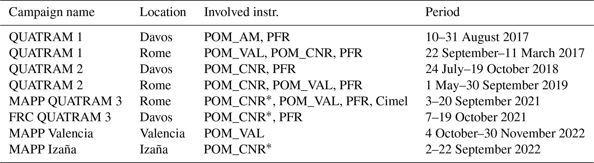
The PFR instrument, manufactured by PMOD/WRC, is used in the GAW AOD network, and it is a classic sun photometer equipped with 3 to 5 nm bandwidth interference filters (368, 412, 500, and 863 nm) and a field of view of 2.5°. The detector unit is held at a constant temperature of 20 °C by an active Peltier system. Dielectric interference filters manufactured with the ion-assisted deposition technique are used to ensure significantly larger stability in comparison to those manufactured with classic soft coatings. The PFR was designed for long-term stable measurements; therefore, the instrument is hermetically sealed with an internal atmosphere that is slightly pressurized (2000 hPa) with dry nitrogen. The Cimel CE 318 standard AERONET instrument is a multi-wavelength automatic sun–sky photometer developed by Cimel Electronique, measuring direct solar irradiance and sky radiance at nine bands (340, 380, 440, 500, 675, 870, 937, 1020, and 1640 nm) with 2–10 nm FWHM and a field of view of 1.3° (Torres et al., 2013). The detector is not thermostated, and corrections are performed a posteriori.

The datasets used in this work are from the campaigns held at two mountain sites, Davos (46.814° N, 9.846° W; 1588.4 m a.s.l.) and Izaña (28.309° N, 16.499° E; 2373.0 m a.s.l.), and at two urban sites, Rome (41.902° N, 12.516° W; 83.0 m a.s.l.) and Valencia (39.508° N, 0.418° E; 60.0 m a.s.l.). The periods of the campaigns are also listed in Table 1.

The QUAlity and TRaceability of Atmospheric aerosol Measurements (QUATRAM) campaigns (Campanelli et al., 2018; http://www.euroskyrad.net/quatram.html, last access: 7 August 2024) are organized by the Institute of Atmospheric Sciences and Climate of CNR (Italy) and the Physikalisch-Meteorologisches Observatorium Davos/World Radiation Center (PMOD/WRC). They are aimed at evaluating the homogeneity and comparability among measurements performed by equipment of different international networks and/or manufactures, as well as at assessing the accuracy of the new on-site calibration procedures. The instruments attending the campaigns and involved in this study are listed in Table 1. The approach of the campaigns consists of performing a calibration transfer from a primary master PFR of the PMOD/WRC to the other instrumentation, of the evaluation of the on-site calibration procedures, and of the comparison of AODs at the common wavelengths. They were held at urban (Rome) and mountain (Davos) sites to consider different atmospheric turbidity and aerosol optical characteristics. The QUATRAM 3, held in Davos in 2021, was hosted by the Fifth WMO Filter Radiometer Comparison (FRC-V) (WMO, 2023). QUATRAM campaigns are used in this study to evaluate the long-term differences between on-site calibrations and PFR transfer, as described in Sect. 3.7.2.

The Izaña and Valencia campaigns were held in the framework of the Metrology for Aerosol Optical Properties (MAPP) project with the purpose of generating data to be used for a development of a comprehensive uncertainty budget for aerosol optical properties from remote sensing techniques and to determine the top-of-atmosphere solar and lunar spectra.

3 Estimation of the solar calibration constant

Three methods for the estimation of V₀ are analyzed in the following sections: the in-lab calibration at PTB, the transfer of calibration among instruments, and the on-site procedures. The evaluation of the performance of the SKYNET on-site calibration procedures was assessed by comparing the retrieved constants against

• a.

  the laboratory calibrations performed by the Physikalisch-Technische Bundesanstalt (PTB), Germany; the Aalto University, Finland; and the PMOD, Switzerland; and

• b.

  the transfer of calibration from PFR and Cimel to Prede POM instruments operating simultaneously.

3.1 The laboratory calibrations at PTB

The two sun–sky radiometers, POM_VAL and POM_CNR, were calibrated at PTB with respect to their spectral irradiance responsivities. The calibrations were accomplished using the tunable laser-based facility, TUnable Lasers In Photometry (TULIP). The TULIP facility, shown in Fig. 1, has recently been upgraded with a laser system based on an optical parametric oscillator (OPO) operating in pulsed mode with a pulse length of 2.5 ps and a repetition rate of 80 MHz. The laser wavelength is automatically tunable throughout the spectral range from 230 to 2300 nm. A high-accuracy laser spectrum analyzer (LSA) is used to monitor the laser wavelength, which is stable within 10 pm during a typical measurement sequence. The spectral bandwidth of the laser radiation is wavelength dependent and varies between 0.2 and 0.7 nm in the visible spectral range. The centroid values of the measured laser spectrum are used as the wavelengths of the corresponding spectral responsivity values.

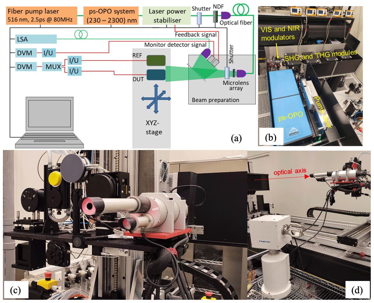
Figure 1 TULIP setup at PTB: (a) schematic representation of the setup including the optical parametric oscillator (OPO) system, variable neutral-density filter (NDF), reference (REF) and detector under test (DUT), current-to-voltage converter ($I/U$), multiplexer (MUX), digital voltage meter (DVM), and laser spectrum analyzer (LSA); (b) a picture of the ps-OPO system; (c) a picture of POM and reference detectors installed on the translation stage system; (d) a side view of the POM instrument facing the beam shaping optics inside the enclosure.

A spatially homogeneous non-polarized field with temporally stabilized irradiance values is produced by beam shaping optics based on a micro-lens array. The amplitude stabilization of the output radiation from the laser system is achieved using two liquid crystal display (LCD)-based modulators inserted in the signal and idler beams of the OPO, before the second and third harmonic (SHG and THG) modules of the laser system. The feedback signals for the control circuits of the intensity modulators are taken from Si and InGaAs photodiodes irradiated by a fraction of the radiation field formed by the micro-lens array. In this way, the irradiance values at the measurement plane are stabilized to a level of a few parts in 10⁴. The homogeneity of the generated field is within a few parts in 10³. Spectral irradiance responsivity calibrations are made in such a field by comparing the signal of a device under test (DUT) to that of a reference detector (REF), positioned sequentially at the same position in the measurement plane. The spectral irradiance responsivities of the reference detectors built of Si and InGaAs photodiodes for the visible and near-infrared wavelengths, respectively, are obtained through a chain of calibrations from a primary cryogenic radiometer and from the calibrated areas of the precision radiometric apertures used with the reference detectors.

The spectral irradiance responsivity calibrations of the sun photometers were made at ca. 1.5 m from the micro-lens array. At this distance, the illuminated area of the micro-lens array seen by the radiometers subtends ca. 0.3°. The entrance apertures of the sun photometers were aligned perpendicular to the optical axis of the TULIP setup. The angular orientation of the POM instruments in the setup was optimized by tilting and rotating to maximize the signal. This ensured that the central part of the field of view was illuminated by the laser-induced irradiation field. The numbers of the digital signals (DN) from the POM instruments were requested and read via a serial port of the TULIP control PC using respective software commands. During the measurements it was not possible to select the internal gain settings of the POM instruments. These settings are managed by the instrument firmware. It was therefore also not possible to verify the gain values during the laboratory calibrations and their respective contributions to the measurement uncertainties.

The results of the calibrations of all the channels of the two instruments are shown in Fig. 2. The bandpass functions of the spectral channels were found to match the nominal filter function well. Only the 940 nm channel of POM_VAL showed a large deviation. Most of the spectral channels were confirmed to block the out-of-band radiation to the level of $\mathrm{1}\times {\mathrm{10}}^{-\mathrm{8}}$ throughout the whole spectral range.

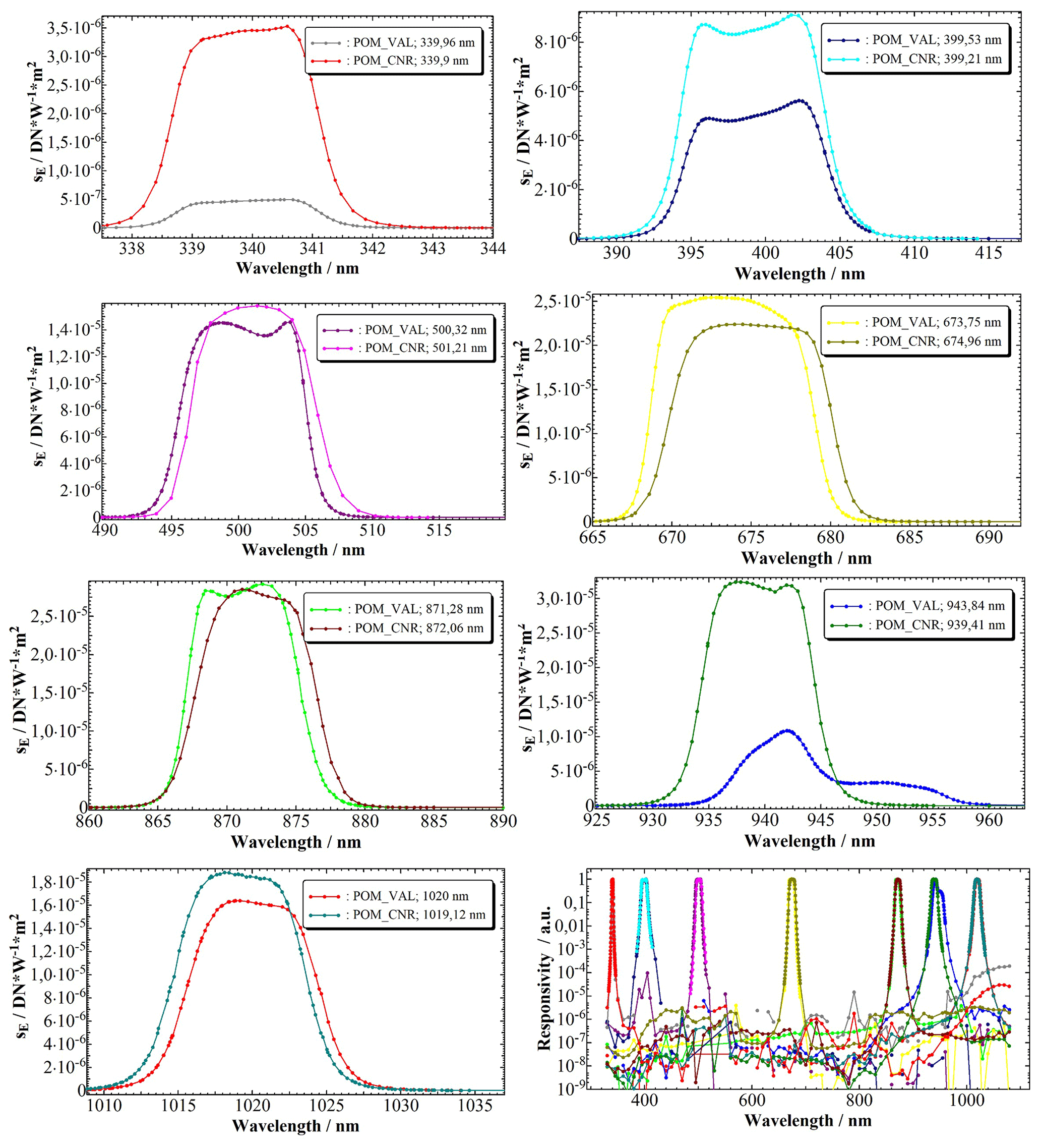
Figure 2 Measured spectral irradiance responsivities of all channels of the sun photometers and their normalized values displayed on a logarithmic scale.

The uncertainty analysis of the spectral irradiance measurements was accomplished by a Monte Carlo method according to Evaluation of measurement data – Supplement 1 to the “Guide to the expression of uncertainty in measurement” – Propagation of distributions using a Monte Carlo method (BIPM et al., 2008) using the measurement equation including all relevant uncertainty contributions. The known uncertainty components include the uncertainty of the reference detector responsivity, its aperture area, stability and LSA-based measurement of the laser wavelength, spatial homogeneity of the laser-generated field, the temporal stability of the irradiance values, laser bandwidth variation, and positioning of the detectors in the plane of measurements. For the latter uncertainty contribution, the position of the effective radiometric aperture of the measured detectors along the optical axis must be known. In the case of the reference detectors with well-defined mechanical apertures, their position can be determined with an accuracy of better than 0.1 mm. However, the position of radiometrically limiting apertures of sun photometers with lens optics cannot be measured directly as they are behind the lens. In this case, they were determined through distance variation with much higher resulting uncertainties. For the Prede POM sun photometers, the positions of the effective apertures could be determined with estimated standard uncertainties of 3 mm. The respective uncertainty contribution also dominated the uncertainty of the spectral irradiance responsivity calibrations of the filter radiometers (Fig. 3).

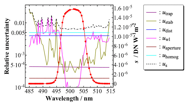
Figure 3 Example of spectrally dependent uncertainty components of spectral irradiance responsivity measurements of the 500 nm channel of POM_CNR. The relative uncertainties on the left axis represent components due to the reference detector (u_trap), temporal irradiance stability (u_stab), detector positioning (u_dist), laser wavelength (u_wl), aperture area (u_aperture), spatial homogeneity (u_homog), and the resulting standard uncertainty of the measurements (u_s).

It should be noted that the uncertainty analysis only included the uncertainty components identified during the laboratory calibrations under the respective measurement conditions. As mentioned previously, uncertainty contributions from internal gain values of the POM instruments could not be estimated due to the lack of functionality of the instruments for laboratory calibrations. Also, the temperature stabilization of POM_CNR did not work during the calibrations at PTB. The effect of the instrument malfunction on the calibrated responsivity values was not included in the uncertainty analysis. In addition, there may be some other differences between the operating conditions of the instruments during the laboratory calibrations and their use in the field, which could lead to additional uncertainty contributions.

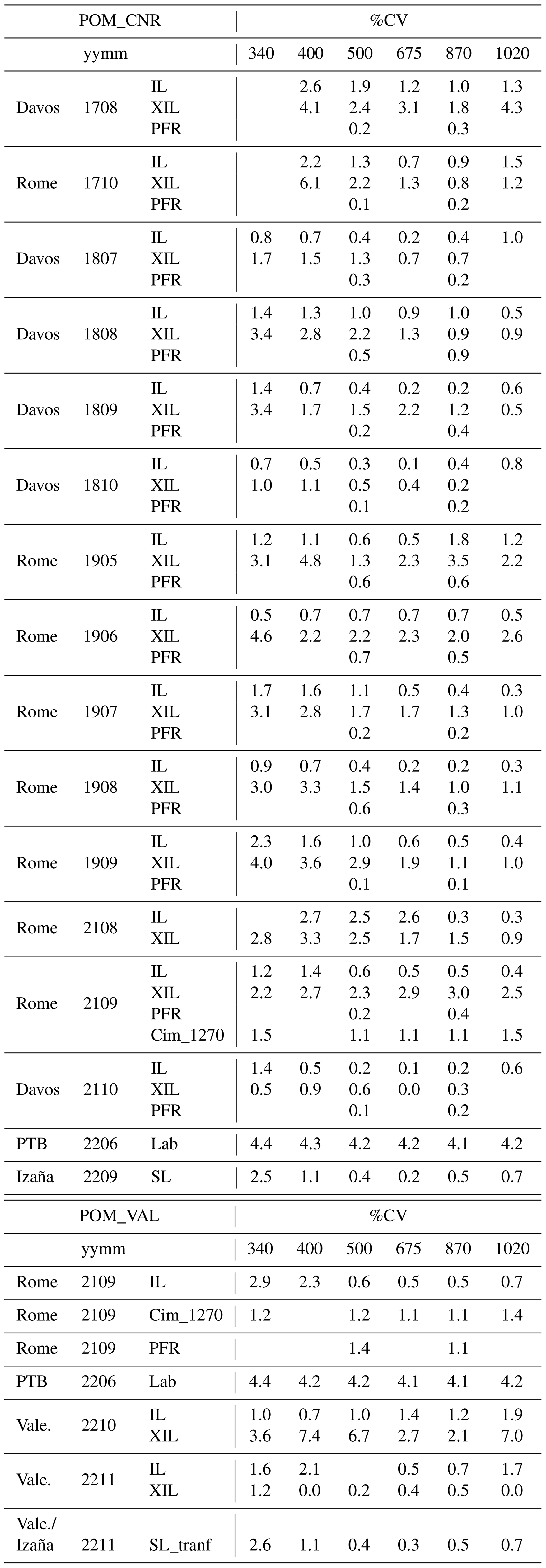
The calibration factors V₀ were obtained a posteriori by integration of the spectral response and the extraterrestrial TSIS spectrum (Coddington et al., 2023). The uncertainties were estimated by quadratic error propagation of the numerical integral. The results are summarized in Table 2, with only the percent differences, and are shown more completely in Tables S1 and S2 in the Supplement.

Table 2 Percent coefficients of variation (%CV) for all the methods and periods for POM_CNR and POM_VAL. When CV is 0, it means that the monthly dataset is composed of only one point. Column three shows the type of method used: IL (improved Langley), XIL (cross-improved Langley), PFR (transfer from the PFR instrument), Cim_1270 (transfer from Cimel), Lab (laboratory calibration), SL (standard Langley), and SL_tranf (transfer from POM_CNR standard Langley).

Within the EMPIR project 19ENV04 MAPP, sun photometers from GAW PFR and AERONET networks were also measured at PTB with respect to their spectral irradiance responsivities. The results of the laser-based calibrations of several sun photometers were verified by additional methodologies for laboratory calibrations. The spectral irradiance responsivities of a PFR and two Cimel instruments determined at the TULIP setup were verified by a calibration against reference standard lamps with traceability to the primary spectral irradiance standard (a high-temperature blackbody). The results agreed well within the uncertainties of the calibrations, i.e., in the range between 0.2 % and 1 %. One Cimel instrument was also calibrated in radiance mode using an integrating sphere source calibrated at PTB for the spectral radiance. These calibration data combined with the field-of-view (FOV) values measured by PMOD yielded spectral irradiance responsivities of the Cimel channels that agreed within 1 % to 2 % with those determined at the TULIP setup in irradiance mode.

The spectral irradiance responsivities of the PRF were combined with the published spectral irradiance at the top-of-atmosphere (TOA) values (QASUMEFTS, λ ≤ 500 nm, and TSIS-1 Hybrid Solar Reference Spectrum, λ > 500 nm) to derive the signal values that would be measured at the TOA. Those values were compared with those obtained by the Langley technique. The agreement between the values was within 0.5 %. Also, the AOD values derived using the laboratory-based calibration of the PFR were in agreement with those from the Langley-based calibration (Kouremeti et al., 2021; Gröbner et al., 2023).

For the three Cimel instruments calibrated at PTB, the agreement between the calculated TOA values and those derived by the Langley extrapolation technique was in the range of 1 % to 5 %, with the discrepancies systematically increasing towards the short-wavelength channels. Thus, for all instruments, the results of the in-lab calibrations were consistent within their respective uncertainties, regardless of the calibration methods used.

3.2 The standard Langley (SL) method for POM_CNR

The standard Langley method (Shaw, 1976) is the most common procedure adopted to calculate the solar calibration constant. It is based on the Beer–Lambert law (Eq. 1):

$$\begin{array}{}\text{(1)}& \begin{array}{rl}& V=V_{\mathrm{0}}\exp \left(-m_{\mathrm{0}}\mathit{\tau }\right)\text{or}\\ & \ln V=\ln V_{\mathrm{0}}-m_{\mathrm{0}}\left({\mathit{\tau }}_{\mathrm{gas}}+{\mathit{\tau }}_{\mathrm{R}}\right)-m_{\mathrm{0}}{\mathit{\tau }}_{\mathrm{ext}},\end{array}\end{array}$$

where V is the direct solar irradiance measured on the ground; m₀ is the optical air mass as the inverse of the cosine of the solar zenith angle; τ_ext is the extinction AOD; and τ_gas and τ_R are, respectively, the gas absorption optical depth and the molecular (Rayleigh) scattering optical depth.

The standard Langley method consists of the retrieval of V₀ by the fit of y vs. x in Eq. (2), assuming that optical depth due to aerosol is constant, as it happens performing the measurements at high altitude (i.e., above the boundary layer, where AOD is low, and its absolute variability is also very low).

$$\begin{array}{}\text{(2)}& \begin{array}{rl}& y=a_{\mathrm{SL}}+b_{\mathrm{SL}}x,\\ & \text{where}x=m_{\mathrm{0}}\\ & y=\ln V+m_{\mathrm{0}}\cdot \left({\mathit{\tau }}_{\mathrm{gas}}+{\mathit{\tau }}_{\mathrm{R}}\right)\end{array}\end{array}$$

The linear fitting provides intercept a_SL=ln  V₀ and slope $b_{\mathrm{SL}}=-\mathit{\tau }$.

This method is used for measurements taken at the Izaña observatory by POM_CNR. The following criteria are used to filter the data: (i) only data for m₀≥2 and ≤5 are considered; (ii) using a and b parameters retrieved from the fit, y_fit is obtained from Eq. (2) and the residuals are calculated for each point as y−y_fit; their RMSD is calculated and if it is > 0.006, the mean of residuals is calculated, and points for which residual is greater than mean value are removed; a new fit is then performed and the process is repeated until RMSD < 0.006 is obtained; (iii) a special criterion is applied for 340 nm, where data points were only selected for m<2. The primary reason for choosing this air mass threshold is its sensitivity towards molecules (Rayleigh scattering). Selecting higher optical mass means light gets scattered more and can cause errors. A similar strategy is also used in Estellés et al. (2004). The selected series were considered only if the number of data points was greater than 50. After a visual inspection, a period of 3 d of the Izaña campaign (7, 8, and 9 September 2022) was very stable and showed minor fluctuations. Calibration values were calculated for these 3 d both in the morning (before 13:00 UTC) and afternoon for each wavelength with the air mass limit between 2 and 5.

Uncertainty was determined as the standard deviation of the calibration values calculated for 3 d in morning and evening (six plots). The mean was taken as the final calibration value. The results are summarized in Table 2, with only the percent differences, and are shown more completely in Tables S1 and S2.

3.3 The improved Langley methods (IL-XIL) for POM_CNR and POM_VAL

Based on the above-described Langley method, the formula of the improved Langley method is expressed as follows:

$$\begin{array}{}\text{(3)}& \begin{array}{rl}& y=a_{\mathrm{IL}}+b_{\mathrm{IL}}x,\text{where}\\ & x=m_{\mathrm{0}}\mathit{\omega }{\mathit{\tau }}_{\mathrm{ext}}=m_{\mathrm{0}}{\displaystyle \frac{{\mathit{\tau }}_{\mathrm{sca}}}{{\mathit{\tau }}_{\mathrm{ext}}}}{\mathit{\tau }}_{\mathrm{ext}}=m_{\mathrm{0}}{\mathit{\tau }}_{\mathrm{sca}}\text{and}\\ & y=\ln V+m_{\mathrm{0}}\cdot \left({\mathit{\tau }}_{\mathrm{gas}}+{\mathit{\tau }}_{\mathrm{R}}\right),\end{array}\end{array}$$

where ω is the aerosol single-scattering albedo (defined as $\frac{{\mathit{\tau }}_{\mathrm{sca}}}{{\mathit{\tau }}_{\mathrm{ext}}}$). The linear fitting provides intercept a_IL=ln  V₀ and slope $b_{\mathrm{IL}}=-\frac{\mathrm{1}}{\mathit{\omega }}$.

The improved Langley plot method (Campanelli et al., 2004, 2007; Nakajima et al., 2020) is the standard calibration method of the SKYNET network, and it was used to calculate the solar calibration constants for both Prede POM sun–sky photometers.

The calibration value, V₀, is retrieved by fitting the natural logarithm of the direct solar irradiance versus the product of m₀ and the scattering optical depth, as retrieved by the SKYRAD 4.2 code (Nakajima et al., 2020), instead of only the air mass as occurs with the standard Langley plot.

As described in Sect. 3.2, the standard Langley assumes that, in the selected time period, the AOD is constant, so data must be accurately chosen because the result is directly related to the variability of AOD. Shaw (1979, 1983) demonstrated that the linear dependence of AOD on m₀, which means a temporal change in the optical thickness because m₀ depends on time, corresponds to the second-order variation in terms of time. Limiting to the first order and following Eqs. (2) and (3) of Campanelli et al. (2004) AOD can be expressed as the sum of a stable term (AOD₀) and a term indicating the variability (AOD${}_{\mathrm{1}}/m_{\mathrm{0}}$). Equation (1) can be therefore briefly expressed as $\ln V=\ln V_{\mathrm{0}}-{\text{AOD}}_{\mathrm{1}}-m_{\mathrm{0}}{\text{AOD}}_{\mathrm{0}}$. In the standard Langley plot the intercept value contains the variability (ln  V₀−AOD₁), and the retrieved V₀ value has a substantial dependence on the daily variability of AOD. Conversely, in the improved Langley plot, V₀ is retrieved by the fit of ln  V vs. the product of m₀ and the scattering optical depth that includes the variability term. In contrast to the standard method, the intercept V₀ does not depend on the AOD in-day variation if the product ωτ_ext is correctly retrieved by the inversion process.

To now understand the main idea on which this method is based, we define the two observable quantities (for each wavelength λ) important for the sun–sky photometer, the direct solar irradiance in Eq. (1) and the normalized radiance R in Eq. (4):

$$\begin{array}{}\text{(4)}& R\left(\mathrm{\Theta }\right)={\displaystyle \frac{E\left(\mathrm{\Theta }\right)}{\mathrm{\Delta }\mathrm{\Omega }\cdot V\cdot m_{\mathrm{0}}}},\end{array}$$

where Θ is the scattering angle at which the Prede POM takes measurements of the sky diffuse irradiance E, V is direct irradiance, and ΔΩ is the solid view angle of the instrument.

R is determined as the solution of the radiative transfer equation, as in Eq. (5) in the almucantar geometry for a one-layer plane-parallel atmosphere, where P is the phase function, and q indicates the multiple-scattering contribution:

$$\begin{array}{}\text{(5)}& R\left(\mathrm{\Theta }\right)=\mathit{\omega }{\mathit{\tau }}_{\mathrm{ext}}P\left(\mathrm{\Theta }\right)+q\left(\mathrm{\Theta }\right)={\mathit{\tau }}_{\mathrm{sca}}P\left(\mathrm{\Theta }\right)+q\left(\mathrm{\Theta }\right).\end{array}$$

Thus, normalized radiance R is approximately assumed to be the product of τ_sca and P; τ_sca is derived via the inversion process (e.g., SKYRAD 4.2) of volume size distribution from the normalized radiance in the aureole region with scattering angles 3° < Θ < 30° (Nakajima et al., 2020), keeping the complex refractive index fixed, and it is used in the improved Langley method for obtaining the intercept V₀. Note that the aerosol optical depth for scattering (in x in Eq. 3) is potentially retrieved more accurately than the optical depth for extinction τ_ext. To understand the reason, it must be considered that the volume size distribution is roughly obtained by only direct radiation information because of the limited information content of the extinction kernel function (Tonna et al., 1995; their Fig. 4). On the other hand, for the sky radiance measurements in the range 3° < Θ < 30°, the scattering kernel functions (Tonna et al., 1995; their Fig. 4) have reliable information content (approximately within 1 < 2$\mathit{\pi }r/\mathit{\lambda }$ < 60, which means that 0.05 < r < 10 µm for our wavelength set) that is sufficient for deriving the volume size distribution and reliably reconstructing the connected quantities R, P, and ωτ_ext. The radiance in the aureole region is also less sensitive to the refractive index (Tanaka et al., 1983). Therefore, the use of R in Eq. (5) to obtain ωτ_ext., i.e., scattering optical thickness, is the best way to analyze data.

From R and V data collected each month, two V₀ values a day are calculated with data taken in the morning and in the afternoon, and the V₀ monthly means are quality-checked according to Campanelli et al. (2007) and summarized as follows: (i) the values of ωτ_ext obtained from the SKYRAD 4.2 code inversion with accuracy lower than 7 % are rejected; the accuracy is estimated as the percent differences between the measured and retrieved radiance R, averaged over all the wavelengths and scattering angles; (ii) only the measurements taken for m₀< 3.0 and $\mathrm{1}/\mathit{\omega }$ > 0 and ≤ 2 are selected; (iii) all the values of V₀ found for τ_ext (500 nm) ≥ 0.4 are rejected; (iv) a minimum number of 10 points is used in each morning and afternoon fit.

The rejection of τ_ext (500 nm) values greater than 0.4 is not in contradiction with the AERONET strategy, where the retrieval of ω is performed only for τ_ext > 0.4 (AERONET web page, 2024; Holben et al., 2006); otherwise, ω and other properties are not included in the AERONET L2 analysis, because the purpose of this selection for IL is different. In fact a potential problem in this procedure is that the refractive index is kept fixed. The aureole region has information for volume size distribution but not for refractive index, as mentioned previously, and this allows us to retrieve τ_sca. However, a high τ_ext makes a high multiple-scattering contribution (q(Θ) in Eq. 5) and results in a greater error in retrieving τ_sca with a fixed refractive index.

Once the filtered monthly V₀ series are obtained, the outliers and short-term variations related to the method itself are filtered using the Chauvenet criterion (Young, 1962), which rejects points out of 2 times the standard deviation (SD​​​​​​​), and a three-point moving-average technique. Finally, if at least three values remain and the ratio between their SD and mean (coefficient of variation, CV) is < 3 %, the monthly mean V₀ value is calculated. The uncertainty related to this value is given for each wavelength by the CV coefficient. The results are summarized in Table 2, with only the percent differences, and are shown more completely in Tables S1 and S2.

In the real observations, it is difficult to separate natural variations and inversion errors of ωτ_ext, and thus undesired inversion errors that lead the IL method to an underestimation of the fitting parameters in the case of large aerosol retrieval errors can be included (Nakajima et al., 2020). A new solution to this problem is tested, named the cross-IL method (XIL), which exchanges the role of x and y in the regression analysis as described in Eq. (6):

$$\begin{array}{}\text{(6)}& x=a_{\mathrm{XIL}}+b_{\mathrm{XIL}}y.\end{array}$$

The linear fitting provides slope $b_{\mathrm{XIL}}=\frac{\mathrm{1}}{b_{\mathrm{IL}}}=-\mathit{\omega }$ and intercept $a_{\mathrm{XIL}}=-\frac{a_{\mathrm{IL}}}{b_{\mathrm{IL}}}=\mathit{\omega }\ln V_{\mathrm{0}}$.

The selection of data for this method is performed using the threshold of 0.05 for the fitting error, assuming that retrieval errors on ω and τ from SKYRAD are within 9 % (Nakajima et al., 2020). Monthly V₀ and the corresponding percent coefficients of variation (%CV) are then calculated. The results are summarized in Table 2, with only the percent differences, and are shown more completely in Tables S1 and S2. Some examples of XIL and IL plots are shown for 340 nm in Figs. S1 and S2t in the Supplement.

3.4 The standard Langley method transfer from POM_CNR to POM_VAL

The calibration of the Prede POM_CNR by the standard Langley plot method at the Izaña campaign, in September 2022, was transferred to POM_VAL using data from the QUATRAM3 campaign, in September 2021, as it was the only campaign where both instruments were co-located.

After visual inspection of the signal ratios for the days of September 2021, the days in the intervals 4–9, 11–15, and 17–19 are considered for the calibration transfer.

The transfer procedure consisted of the following steps: (i) data were selected between 09:00 and 13:00 UTC to avoid the rapid change in air mass; (ii) signals within 30 s between POM_VAL and POM_CNR were considered; (iii) V₀ for POM_VAL was calculated following Eq. (7),

$$\begin{array}{}\text{(7)}& {\displaystyle \frac{V_{\mathrm{0}}^{\mathrm{POM}\mathrm{\_}\mathrm{UV}}}{V_{\mathrm{0}}^{\mathrm{POM}\mathrm{\_}\mathrm{CNR}}}}={\displaystyle \frac{V^{\mathrm{POM}\mathrm{\_}\mathrm{UV}}}{V^{\mathrm{POM}\mathrm{\_}\mathrm{CNR}}}};\end{array}$$

(iv) values that are more than 3 scaled median absolute deviations away from the median are assumed to be outliers and deleted; (v) daily $V_{\mathrm{0}}^{\mathrm{POM}\mathrm{\_}\mathrm{UV}}$ medians are calculated, and 2 SD of the $V_{\mathrm{0}}^{\mathrm{POM}\mathrm{\_}\mathrm{UV}}$ series is calculated; if 2 SD is larger than 0.5 % of the daily V₀ median, all data outside 2 SD are removed; the process is repeated until 2 SD becomes equal to or smaller than 0.5 % of the daily $V_{\mathrm{0}}^{\mathrm{POM}\mathrm{\_}\mathrm{UV}}$ median or standard deviation and median values become equal in continuous iteration; (vi) after visual inspection, only days which were stable were selected, resulting in the exclusion of the days stated previously.

To calculate the uncertainty of the transferred calibration values, the equation below was used, and we account for uncertainties on the master instrument calibration and the standard deviation of the signal ratios, which are sensitive to changes in AOD:

$$\begin{array}{}\text{(8)}& \begin{array}{rl}& u_{\mathrm{rel}}\left(V_{\mathrm{0}}^{\mathrm{POM}\mathrm{\_}\mathrm{UV}}\right)=u\left(V_{\mathrm{0}}^{\mathrm{POM}\mathrm{\_}\mathrm{UV}}\right)/V_{\mathrm{0}}^{\mathrm{POM}\mathrm{\_}\mathrm{UV}}\\ & =\sqrt{{\left({\displaystyle \frac{u\left(V_{\mathrm{0}}^{\mathrm{POM}\mathrm{\_}\mathrm{CNR}}\right)}{V_{\mathrm{0}}^{\mathrm{POM}\mathrm{\_}\mathrm{CNR}}}}\right)}^{\mathrm{2}}+{\left({\displaystyle \frac{\text{SD}\left(\text{SR}\right)}{\text{SR}}}\right)}^{\mathrm{2}}},\end{array}\end{array}$$

where u_rel is the relative uncertainty, $V_{\mathrm{0}}^{\mathrm{POM}\mathrm{\_}\mathrm{UV}}$ is the mean of the calibration values series and $u(V_{\mathrm{0}}^{\mathrm{POM}\mathrm{\_}\mathrm{UV}}$) is the associated uncertainty, and $V_{\mathrm{0}}^{\mathrm{POM}\mathrm{\_}\mathrm{CNR}}$ is the calibration factor and $u(V_{\mathrm{0}}^{\mathrm{POM}\mathrm{\_}\mathrm{CNR}}$) is the associated uncertainty. This uncertainty was estimated as the SD of the six calibration values obtained by the six plots used in Sect. 3.2, SR is the ratio of signals ($\frac{V^{\mathrm{POM}\mathrm{\_}\mathrm{UV}}}{V^{\mathrm{POM}\mathrm{\_}\mathrm{CNR}}}$), and SD(SR) is the standard deviation of the ratio of the signals available for the calibration. The results are summarized in Table 2, with only the percent differences, and are shown more completely in Tables S1 and S2.

3.5 The calibration transfer from the PFR to POM_CNR and POM_VAL

The transfer of calibration from two reference PFR photometers of the PMOD, one located in Davos and the other in Rome, was carried out for both POM_CNR and POM_VAL during the QUATRAM campaigns.

The transfer is based on the ratio of Eq. (9) for the two instruments, POM and PFR:

$$\begin{array}{}\text{(9)}& {\displaystyle \frac{V_{\mathrm{0}}^{\mathrm{POM},\mathrm{TR}}}{V_{\mathrm{0}}^{\mathrm{PFR}}}}={\displaystyle \frac{V^{\mathrm{PFR}}}{V^{\mathrm{POM}}}},\end{array}$$

where V^PFR and V^POM are the solar direct irradiance measured by the two instruments, $V_{\mathrm{0}}^{\mathrm{POM},\mathrm{TR}}$ is the unknown solar calibration constant of the POM instrument, and $V_{\mathrm{0}}^{\mathrm{PFR}}$ is the known calibration constant of the PFR to be transferred. For QUATRAM 3 in Rome, days from 6 to 8 and from 11 to 14 of September 2021 were considered.

Signal ratios $\frac{V^{\mathrm{PFR}}}{V^{\mathrm{POM}}}$ were taken using measurements that are within 30 s time difference, and cloudy conditions were removed, together with ratio outliers. Values outside of the interval time 09:00–13:00 UTC were rejected. From Eq. (9) the time series of $V_{\mathrm{0}}^{\mathrm{POM},\mathrm{TR}}$ was limited to the following: (i) choose only those days for which at least 20 measurements in 1 h are available; (ii) calculate the daily V₀ medians and compare each with 2 SD of the day's V₀ values; if 2 SD is larger than 0.5 % of the daily V₀ median, remove all data outside 2 SD; repeat until 2 SD becomes equal to or smaller than 0.5 % of the daily V₀ median; when this is accomplished, if the day's measurements have dropped below 20, the day is excluded. Daily medians of the remaining values are calculated, and then a monthly mean $V_{\mathrm{0}}^{\mathrm{POM},\mathrm{TR}}$ is estimated. The SD of the monthly mean values is assumed to be the uncertainty. The results are summarized in Table 2, with only the percent differences, and are shown more completely in Tables S1 and S2.

For the transfer to POM_VAL during QUATRAM 3, the same procedure was applied, but the selected days are from 6 to 9 and from 11 to 14 of September 2021.

The uncertainties were estimated as in other transfer cases by assuming a nominal uncertainty of the PFR calibration of 1 %. Results for both instruments are summarized in Table 2, with only the percent differences, and are shown more completely in Tables S1 and S2.

The same procedure was applied for the QUATRAM 3 in Davos and QUATRAM 1 and 2 at both sites for POM_CNR.

3.6 Calibration transfer from Cimel to POM_CNR and POM_VAL

During QUATRAM 3, a calibration transfer from Cimel instrument no. 1270 was carried out, following the same selection criteria of the transfer from the PFR.

To calculate the total uncertainty of the transferred calibration values, Eq. (8) was used with $V_{\mathrm{0}}^{\mathrm{CIM}}$ as the master instrument and $u(V_{\mathrm{0}}^{\mathrm{CIM}}$) as the associated uncertainty. As the estimated uncertainty is absent for the master instrument, it is assumed to be 1 % of V₀. The results are summarized in Table 2, with only the percent differences, and are shown more completely in Tables S1 and S2.

3.7 Comparisons

3.7.1 Differences between all methods against the reference one

The six calibration methods described in the previous sections in the period of September 2021–November 2022 for the two POM instruments are compared against a reference calibration. The time interval was chosen because the campaigns and laboratory calibrations were performed in this period in the framework of the MAPP project.

For POM_CNR the reference calibration is the standard Langley method performed at Izaña in September 2022, whereas the transfer of this calibration to POM_VAL is the reference value for the latter instrument. However, we need to consider that the frequent shipments of the equipment during this year for the project purpose and the usage could have affected the values of V₀ and probably could be the reason for discrepancies between the SL calibration and the calibrations performed about 1 year earlier. The aging of the instrument, without shipments, can also affect the V₀, but the order of magnitude and amount per year strongly depend on the instrument, and some wavelengths can be more affected than others. For the two instruments used in this work, it is not possible to evaluate a degradation in 1 year and discern it from the shipment's effects, because the equipment was frequently traveling.

The percent difference was calculated with Eq. (10):

$$\begin{array}{}\text{(10)}& \text{Diff}\left(\mathit{\%}\right)={\displaystyle \frac{\left(V_{\mathrm{0}}^{\mathrm{ref}}-V_{\mathrm{0}}^x\right)}{V_{\mathrm{0}}^{\mathrm{ref}}}}\cdot \mathrm{100},\end{array}$$

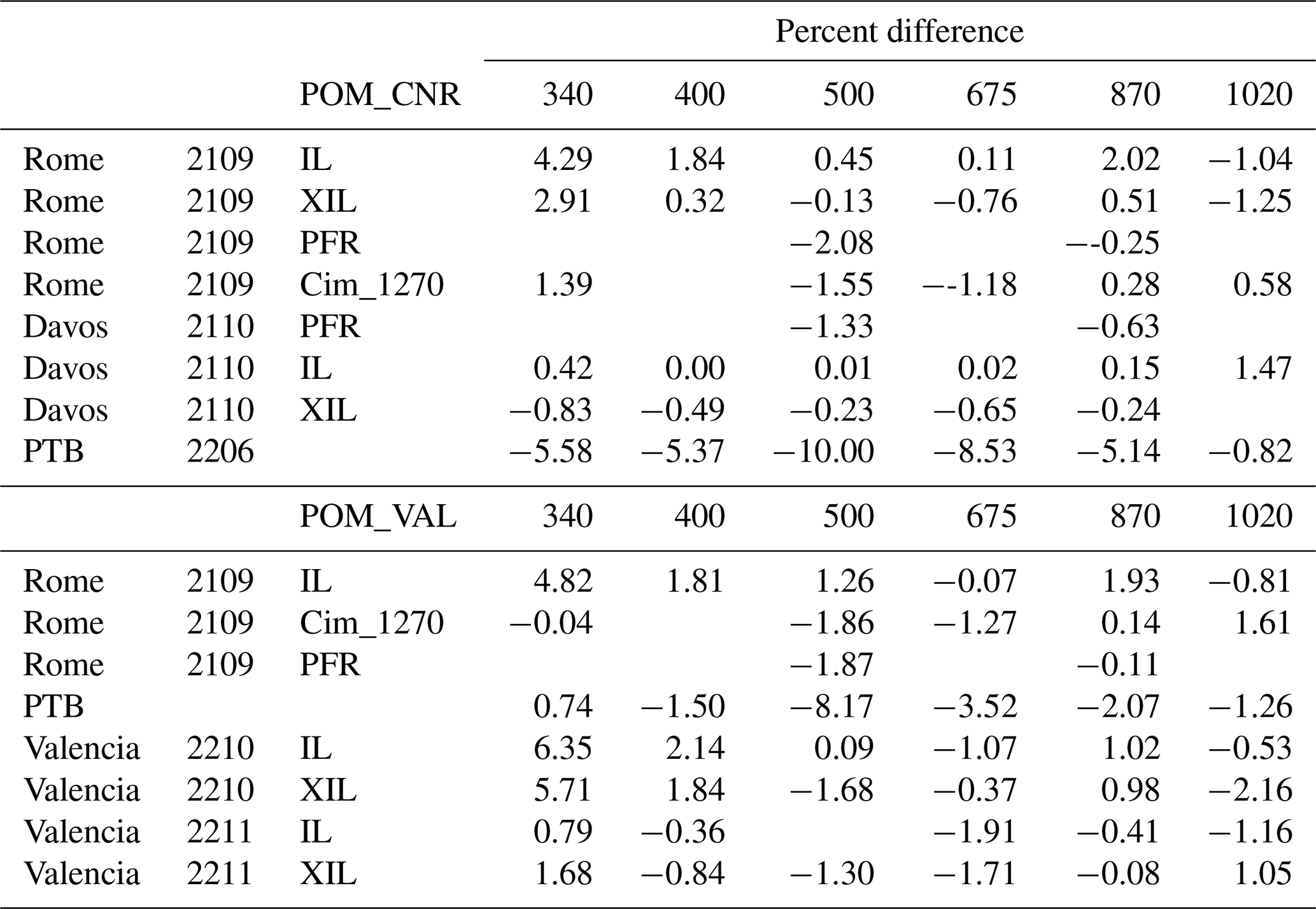
where $V_{\mathrm{0}}^{\mathrm{ref}}$ is the reference value and $V_{\mathrm{0}}^x$ is the calibration obtained with each of the above-described methods. Results are shown in Fig. 4 and Table 3.

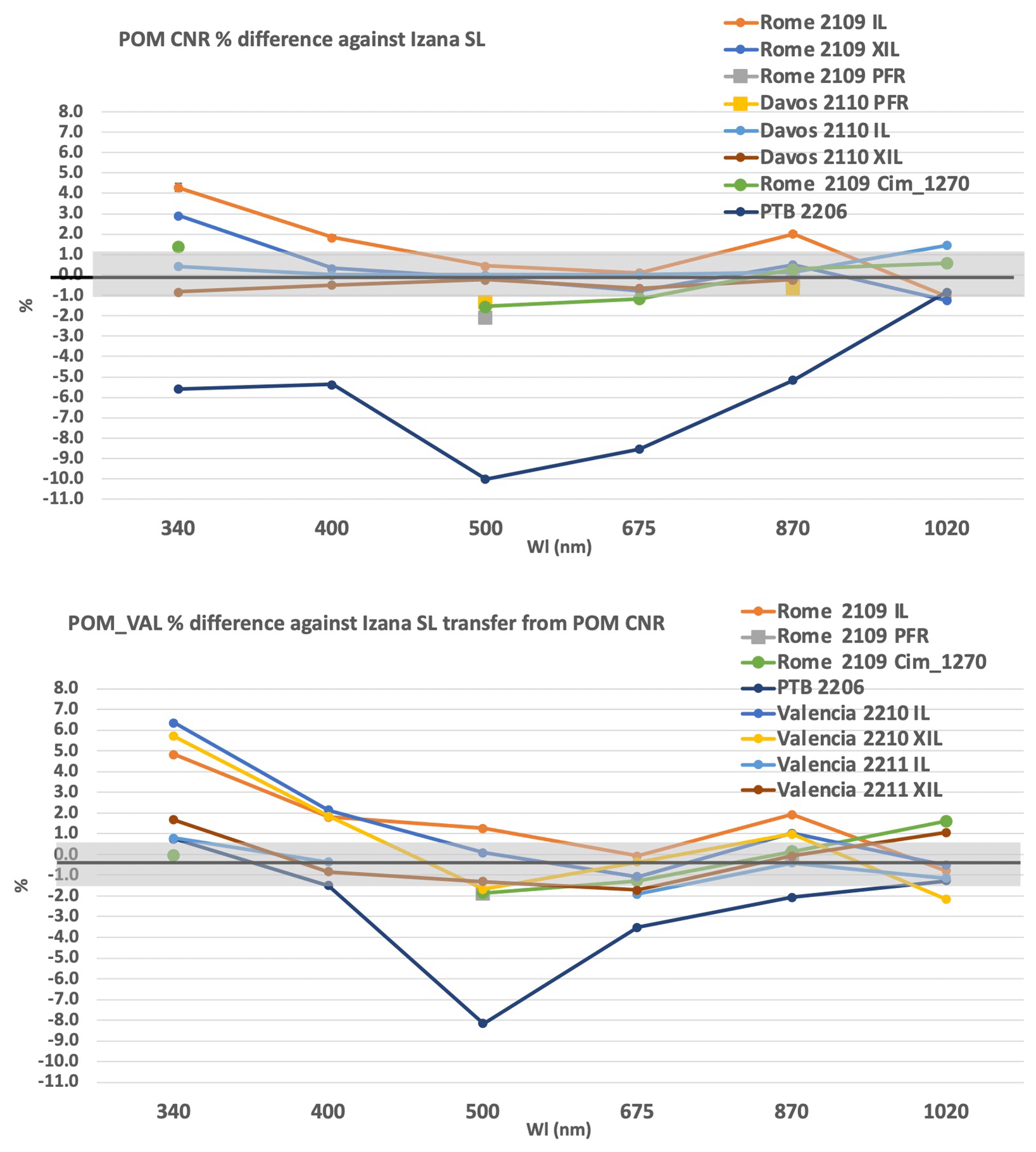
Figure 4 The percent coefficients of variation, calculated as the percent ratio between the standard deviation and the mean values.

Table 3 Percent differences between five calibration methods and the reference one.

For POM_CNR, the agreement is very good with the reference SL, and many of the points are within ±1 %.

The transfer from the Cimel and PFR instruments in Rome and from the PFR instrument in Davos at 500 nm differs by −1.6 %, −2.1 %, and −1.3 %, respectively. The 340 nm wavelength is the one with the most problematic results for the on-site procedures in Rome (with differences of around 4 %). Further studies, not yet published, showed that the 340 nm wavelength is also significantly affected by the assumed surface albedo, and improvements in the agreement are found if, for example, values from the POLarization and Directionality of the Earth's Reflectances (POLDER) radiometer on the ADEOS satellite are considered. More tests are needed to verify this dependence for more sites. Moreover, according to Momoi (2022) the molecular polarization potentially causes calibration errors from IL and XIL at 340 nm, especially in the low-aerosol-loading atmosphere. In fact the SKYRAD pack version 4.2 used for the on-site procedures has an unpolarized (scalar) radiative transfer core forward model that can cause errors of around 8 % on the retrieval of radiance at 340 nm, so it might be one of the reasons for the calibration constant of 340 nm to have errors.

The best agreement is for the IL in Davos with values < 0.5 % at all the wavelengths and 1.5 % at 1020 nm.

For POM_VAL, many points are within ±1 % but less with respect to POM_CNR. The agreement with the reference method for the PTB laboratory calibration shows an improvement, remaining between −1.3 % and −8 % except for the 340 nm wavelength where it is 0.7 %. The transfer from the Cimel and PFR instruments in Rome at 500 nm agrees within −1.9  %, a value comparable with those of POM_CNR. Also, in this case the 340 nm wavelength is the one with the most problematic results for the on-site procedures (with differences of up to 6 %) as explained for POM_CNR.

For the two POM instruments, the comparison with the PTB calibration shows very high underestimations (down to −10 % except for POM_CNR and −8 % for POM_VAL), but at this stage we are not able to provide a specific reason for the discrepancy. It is noteworthy that the agreement between the laboratory calibration and the Langley measurements for the PFR was consistent within the uncertainties. In the case of the Cimel instruments, however, discrepancies increasing towards the short wavelengths and exceeding the uncertainties by a factor of 2–3 were observed. The causes of the discrepancies between the laboratory calibrations and the field measurements of the Cimel and POM instruments are not yet understood.

Focusing on the on-site methodologies, the IL works better in Davos with agreement against SL always below 0.5 % except at 1020 nm, where it increases by up to about 1.5 %. Very good agreement is also found in Valencia in November 2022 – always within 0.8 % except at 500 and 675 nm (within 1.5 %). The similarity between the two cases is probably due to the very low turbidity recorded in this month in Valencia that makes the atmosphere optically more similar to the one in Davos.

The XIL provides a consistent improvement, with values within 1 %, only in Rome for all the wavelengths, but in a very clean atmosphere, as in Davos, it was not possible to retrieve values at 1020 nm, as is done with the IL. This is related to the differences in the data screening criteria between the two methods set up for performing the linear fitting.

3.7.2 Long-term differences between on-site calibrations and PFR transfer

The difference between the on-site calibration methods and the PFR calibration transfer was analyzed in the period of the three QUATRAM campaigns held in Davos and Rome using Eq. (10), with $V_{\mathrm{0}}^{\mathrm{ref}}$ being the transfer from the PFR. V₀ values are shown in Table S1, and the percent differences are shown in Table 4 and Fig. 5.

Table 4 Percent differences between PFR transfer of calibration and the on-site calibration methods at the common wavelengths.

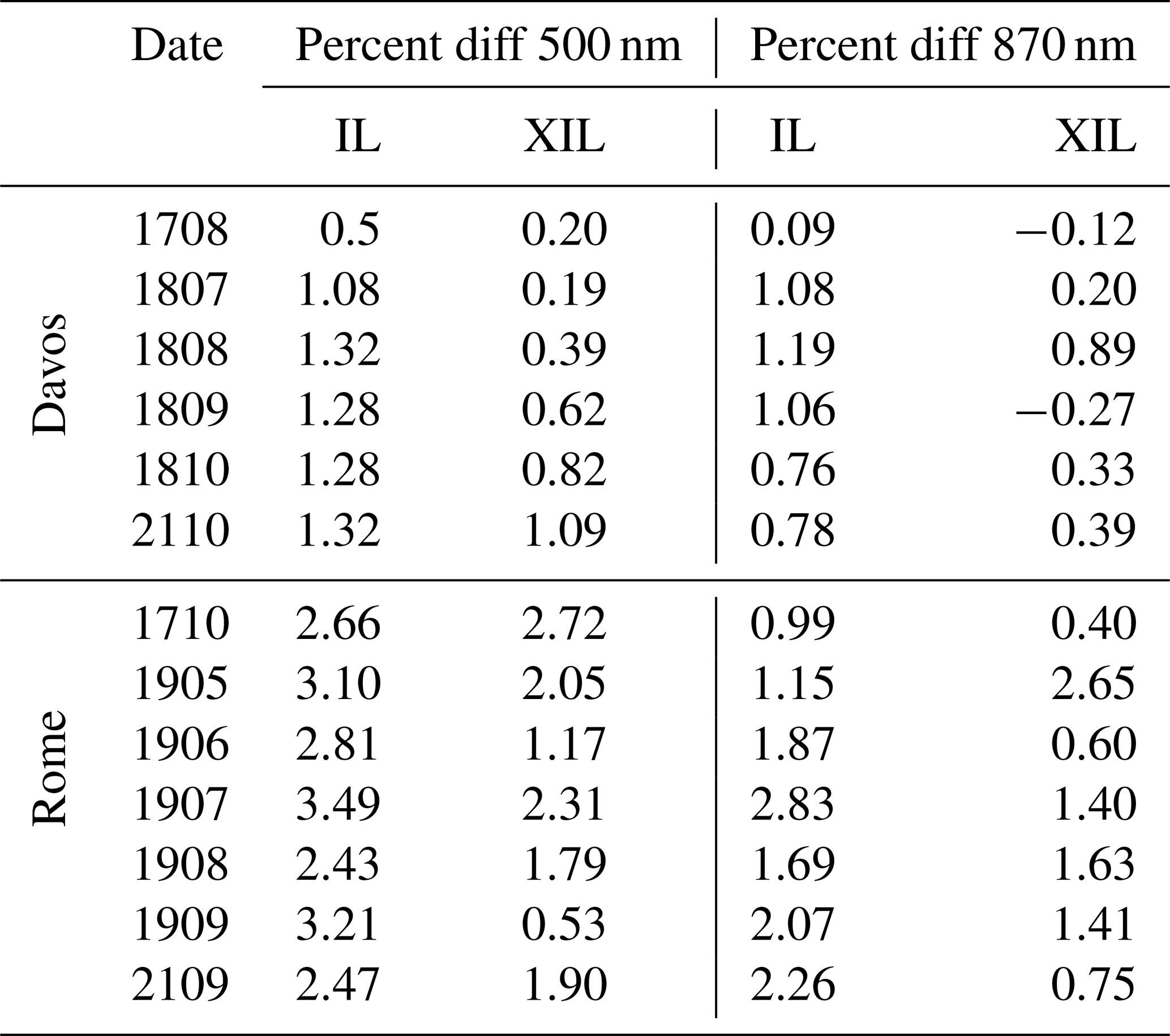
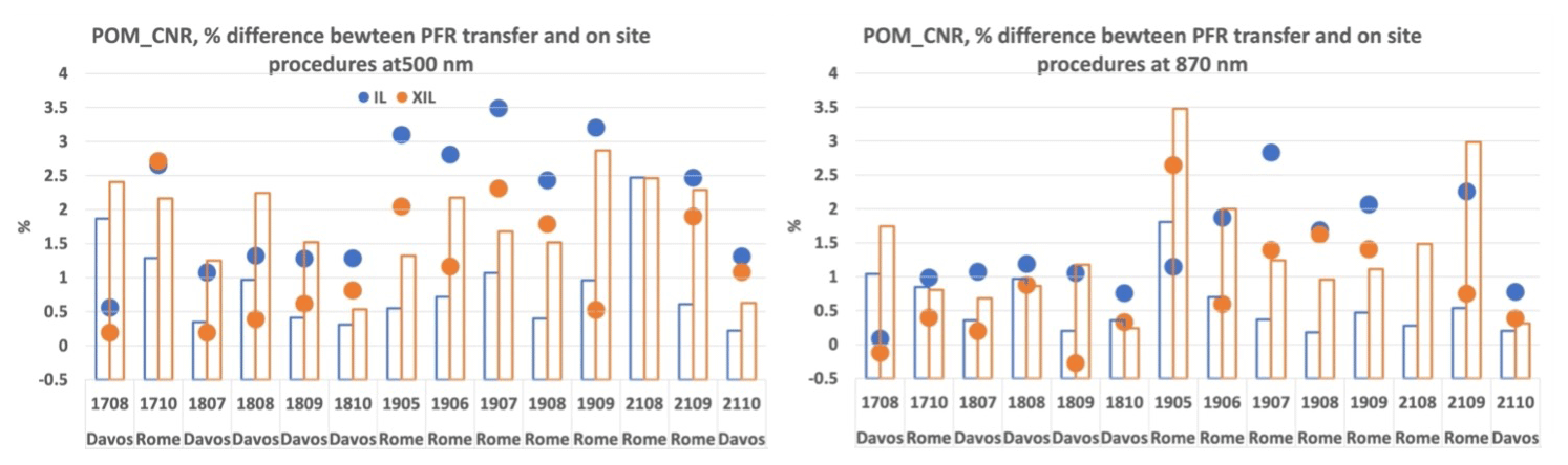
Figure 5 Percent differences between PFR transfer of calibration and the on-site calibration methods at the common wavelengths (circles), as well as the uncertainty %CV of the IL and XIL as in Table 2.

For the IL, the differences are always greater than the uncertainties (%CV) of the method, for both wavelengths, with the exception of Davos in 2017. Values are around 1 % in Davos, and this is an important result for the validation of the IL procedure, confirming the good performance of the improved Langley method on high mountains even if, as shown in Nakajima et al. (2020), the IL accuracy is proportional to the optical thickness of the atmosphere of observation, which is generally low on high mountains. The same result was also obtained by Ningombam et al. (2014). The greater differences are observed in Rome and at 500 nm. At this site the AOD is higher than in Davos, as shown in Fig. 6, and we would have expected a better performance of the on-site methodology. The reason for this result could be related to the fact that in the retrieval of x for performing the fit in Eq. (3), it must be assumed that ωτ_ext=τ_sca and the refractive index do not substantially change during the Langley plot (Campanelli et al., 2004); otherwise, the retrieved optical thickness can include an error caused by the inversion process and also by an improper assumption of the refractive index. In an urban site affected by traffic, such as Rome, we can expect this assumption is not satisfied. Further studies are actually aimed at understanding the possibility of defining some selection criteria for the variability of τ_sca values, particularly in urban sites. Moreover, the use of SKYRAD_MRI (Kudo et al., 2021) instead of SKYRAD 4.2 and the possibility to use only the XIL instead of the IL are under evaluation.

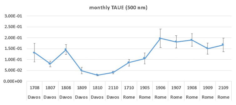
Figure 6 Monthly average and SD of τ_ext at 500 nm from POM instruments listed in Table 1. TAUE is the extinction aerosol optical thickness

For XIL, many differences are within the uncertainties (%CV) of the method, and those higher are closer to the %CV values than in the IL method. XIL improves the agreement particularly in Rome, where the largest difference reduces from 3.5 % to 2.5 % at 500 nm and from 3 % to 1.7 % at 870 nm.

4 Estimation of the solid view angle (SVA)

The SVA is the measure of the field of view of the instrument that can be assumed from the geometry of the telescope. However, several factors contribute to this value: color aberration of the lens and misalignment of the optical axis, which are wavelength dependent; surface nonuniformity of filters that is a randomly function of wavelength; and diffraction at the edges of the lens and nonuniformity of the sensor that are wavelength independent.

This makes it necessary to develop laboratory and on-site methods for correctly estimating SVA values. The methods used in this work are described below.

4.1 Calibration at the laboratory of the Aalto University

The field of view of the Prede POM_CNR was measured at the laboratory of the Aalto University. The measurement setup consists of a two-axis gimbal and a light source. The light source is constructed from an integrating sphere (Gigahertz-Optik type UMBB-300) and a 1 kW Xe lamp. The diameter of the sphere is 300 mm, and the output aperture is limited to 10 mm in diameter. The distance D between the sphere aperture and the axis of rotation was ≈ 1060 mm (Fig. 7). The purpose of the integrating sphere is to obtain a spatially uniform, well-defined light source. The aperture size and the distance D chosen allow the radiometer to see the light source at a solid angle corresponding to the same solid angle where it sees the sun in the field measurements, with an angular diameter of 0.54°.

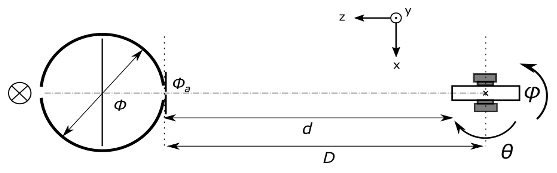
Figure 7 Schematic of the measurement setup. From left to right: a switchable light source, an integrating sphere, and a two-axis gimbal.

The radiometer is mounted on the gimbal and tilted in the desired angle, and the signal amplitude is measured. The setup is built on an optical rail, which enables easy variation of the distance between the gimbal and the light source. The light source and gimbal are fixed in place. The point of rotation of the radiometer was chosen using an x-axis translator and customized elevation blocks installed between the radiometer and the gimbal to set the y direction. The common optical axis of the light source and the radiometer is found by shifting the sphere aperture. The tilt angle range of measurements is [−0.7°, 0.8°] for all channels in both directions, and the step size is 0.1°. The measurement sequence and the data collection are automated using LabVIEW. The integrating sphere and the Xe lamp are shown in Fig. 8.

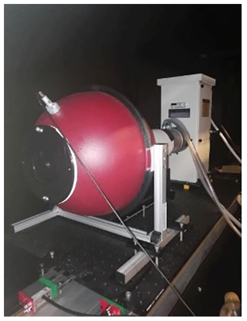
Figure 8 The integrating sphere with an interchangeable aperture and a monitor detector attached. The Xe-lamp housing can be seen behind the sphere. Between the light source and the sphere there is a water-cooled filter to remove the heat at wavelengths above 1000 nm and a lens imaging the arc to the entrance of the sphere. The integrating sphere is of coaxial type with a large screen between the entry and exit ports.

Collected data are used to derive the SVA of the POM instrument following the method of Boi et al. (1999). The solid viewing angle, from the scanning centered at the origin of a local system of rectangular coordinates, is given by Eq. (11):

$$\begin{array}{}\text{(11)}& \mathrm{\Delta }\mathrm{\Omega }=\int \underset{\mathrm{\Delta }A}{\int }{\displaystyle \frac{E(x,y)}{E(\mathrm{0},\mathrm{0})}}\mathrm{d}x\mathrm{d}y,\end{array}$$

where E is the measured intensity (mA) and x and y (in radians) are the polar coordinates that determine the position of the optical axis with respect to the position of the light source. The signals are registered as a function of the (x, y) coordinates, and a circular symmetry for the angular responsivity is assumed. Then a new system of coordinates centered at the center of mass of the angular response is introduced, and the needed parameters are obtained by fitting the measurements.

The results are presented in Table S3, and in Fig. 9 examples of measurements are shown. The left panels display a 2D heat map of the relative signal amplitude as a function of the two tilt angles. The fluctuations of the light source have been taken into account by using correction coefficients obtained from the monitor detector data. The right panels present the signal intensity as a 1D function of distance (r) from the center of mass. Measurements are particularly noisy, and it is probably due to the use of an integrating sphere as a source of light for a photometer, providing low radiation levels to which the instrument has low sensitivity. The measurements should form a plateau at small angles. However, this plateau is disturbed by convolution, as the resolution of the measurement is of the same order of magnitude as the plateau.

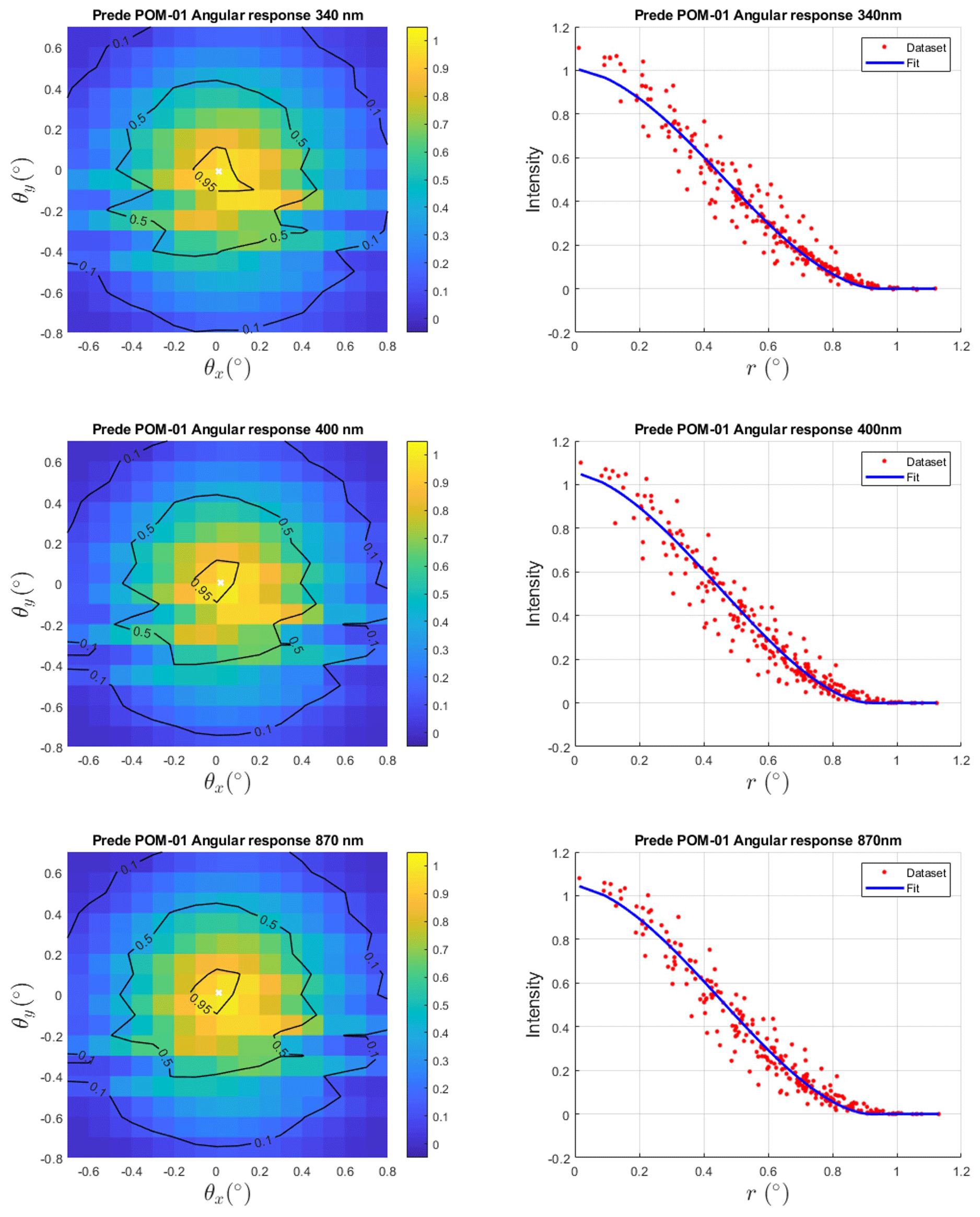
Figure 9 Normalized angular responsivities for POM_CNR. Heat maps on the left have been normalized to the maximum intensity. Graphs on the right have been normalized to the average intensity within r < 0.19°, where the responsivities were assumed to form a plateau.

4.2 Calibration at the laboratory of PMOD

The field-of-view characterization facility at PMOD/WRC consists of a 250 kW Xe-lamp source and a two-axis goniometer system with 0.2 mdeg (millidegree) resolution. The radiation from the Xe lamp shines on a Spectralon reflectance plate which produces a Lambertian radiation distribution. An aperture with a 12 mm diameter is placed in front of the reflectance plate, which is at a distance of 3600 mm from the goniometer system. Thus, the source has an apparent diameter of 0.19°. The field-of-view measurement consists of rotating the radiometer head in both axes from −1.1 to +1.1° in steps of 0.04°. At each position, the average of 10 measurements is stored, and every 100 positions a reference measurement at the nominal center position (0°, 0°) is performed to monitor the stability of the source and of the radiometer. A whole measurement cycle for one channel of the radiometer takes 4.5 h. The FOV of the instrument is obtained by normalizing the measurements at every angle with the reference signal at (0°, 0°), obtained by interpolating the reference measurements to the times of the individual measurements. For the measurements of this radiometer, the variability of the reference measurements varied by 0.38 % during the whole measurement cycle.

Because the source apparent diameter of 0.19° is considerably smaller than the sun (apparent diameter of 0.5°, which is the usual source that this instrument measures), the cross section of the apparent source was not deconvolved from the measurements. Instead, the measurements were convolved with the apparent sun diameter to obtain the corresponding field of view. The slight error made by assuming an initial point source, instead of deconvolving the field of view, was assumed to be less than 0.5 % and added to the uncertainty budget.

The field-of-view measurement of the Prede POM_VAL for the 500 nm channel is shown in Fig. 10. As can be seen in the figure, the region with highest responsivity above 99 % of the maximum is circular, with a diameter of approximately 0.5°.

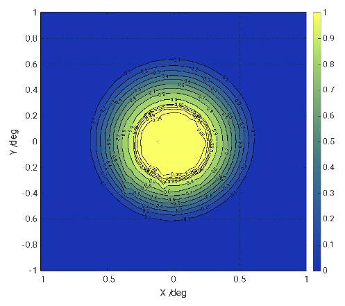
Figure 10 Field-of-view measurement at the 500 nm spectral channel of the Prede POM_VAL. The measurements were normalized to the maximum signal.

From these measurements, the solid view angle Ω of the radiometer at this spectral channel is obtained by Eq. (11).

The standard uncertainty of the solid angle measurements is obtained from the variability of the individual measurements, combined with the variability of the system obtained from the monitoring signals as described above. For the Prede POM_VAL, the standard relative uncertainty of the solid angle determined from these measurements is 0.5 %. Table S3 summarizes the solid angle measurements determined for all spectral channels.

4.3 The solar disk methods

A methodology based on the scanning of the solar disk, described in Boi et al. (1999), is used to determine SVA directly from optical data. It consists of the scanning of the irradiance field around the sun, centered at the origin of a local system of a rectangular domain 2° × 2°; the irradiance is measured for all the channels at 21 × 21 gridded points around the solar disk with an angular resolution 0.1° (Fig. 11a, b). The instrument automatically follows the sun during the scanning, lasting several minutes, and measurements are corrected for the movement of the solar disk. The solid viewing angle, from the scanning centered at the origin of a local system of rectangular coordinates, is given by Eq. (11). An elliptical system of coordinates centered at (0, 0) is introduced to prevent the effect due to the difference between the azimuth and zenith angle steps, and the needed parameters are obtained by fitting the measurements. This method is called solid3m hereafter.

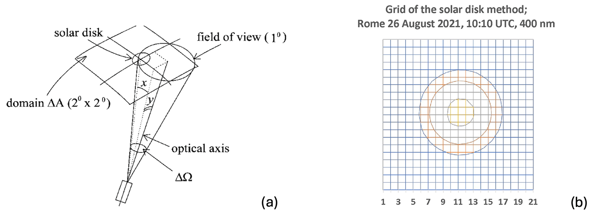
Figure 11 Geometry of the solar disk scanning measurements (a) and 2D image of the scanning (b).

The field of view of a Prede POM is 1°, the size of the sun disk is about 0.5°, and the rectangular domain is 2° × 2°; therefore, the data are taken from the sun for scattering angles up to 1.4° (= (1°) × $\sqrt{\mathrm{2}}$). As shown in Uchiyama et al. (2018) the influence of the direct solar irradiance as a light source extends up to 2.5°. To take this into consideration, the integration of Eq. (11) is performed by linear extrapolation for angles larger than 1.4°. Before starting the data processing, the minimum measured value is subtracted from the measured values, and then the values between 1.4 and 2.5° are extrapolated. However, the subtraction of the minimum measured value largely affects the matrix of measurements in the range of scattering angles [1.0°, 1.4°]. Uchiyama et al. (2018) extended the solid3m method with a new version, hereafter called solid3n, that does not perform this subtraction and extrapolates the values between 1.4 and 2.5° using the data from 1.0 to 1.4°.

SVA was calculated with the solid3m and solid3n methods using measurements taken in Rome and Valencia for POM_VAL and in Rome and Izaña for POM_CNR. The errors (ERR) for the solid3m and solid3n methods are estimated as ($(\text{AM}/\text{ZM})-\mathrm{1}$)², where AM is the measure and ZM is the calculated signals during the fitting phase. Only SVAs having ERR < 0.2 are selected. The mean value over each campaign is assumed to be the final SVA, and its SD is assumed to be the uncertainty associated with the estimation. Results are in Table S3.

The behavior of SVA values over time for the two methods (dashed lines are for solid3m and solid lines are for solid3n) and the two instruments was also analyzed in order to evaluate the stability of the method (Fig. 12). The coefficient of variation for the temporal variation (SD/mean) ranges from 1.1 % to 1.3 % for POM_VAL and from 0.7 % to 0.9 % for POM_CNR, with the exception of 340 nm (2.5 %) and 870 nm (2.0 %) due to the point of 3 September out of the general pattern for 340 and 870 nm.

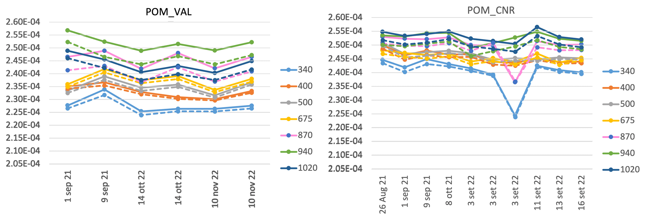
Figure 12 Temporal behavior of SVA values (sr) from solid3m and solid3n methods for POM_VAL and POM_CNR co-located in Rome.

Hashimoto et al. (2012) demonstrated that a SVA underestimation of 1.4 % to 3.7 % can cause an increase in single scattering albedo (SSA) of about 0.03 to 0.04. This estimation was done for SKYRAD pack version 4.2. For SKYRAD_MRI_v2, actually used as the SKYNET standard inversion model, it is expected to be similar because the same forward model, RSTAR, is used in the retrieval, and the relation between SSA and diffuse radiance is the same.

4.4 Comparisons

SVAs calculated with the solid3m and solid3n methods, using measurements taken in Rome, Valencia, Davos, and Izaña, are compared for POM_VAL and POM_CNR instruments against the laboratory calibrations performed in Aalto and PMOD (Table 5 and Fig. 13).

$$\begin{array}{}\text{(12)}& \text{Diff}\left(\mathit{\%}\right)={\displaystyle \frac{\left(\text{SVA}-{\text{SVA}}^{\mathrm{lab}}\right)}{{\text{SVA}}^{\mathrm{lab}}}}\cdot \mathrm{100}\end{array}$$

The solar disk scanning method uses the sun direct irradiance measurements as a light source, whereas the radiance from an integrating sphere is the source at the Aalto laboratory, providing lower radiation levels and noisy measurements as already mentioned in Sect. 4.1. This is probably the reason why for the 340 nm channel of POM_CNR, the wavelength with the lowest intensity level, a large discrepancy is found ranging from 8.62 % to 10.92 % in Rome and Izaña.

Table 5 Differences between SVA values from the on-site calibration methods and the laboratory calibrations for the two POM instruments. Wl is the wavelength.

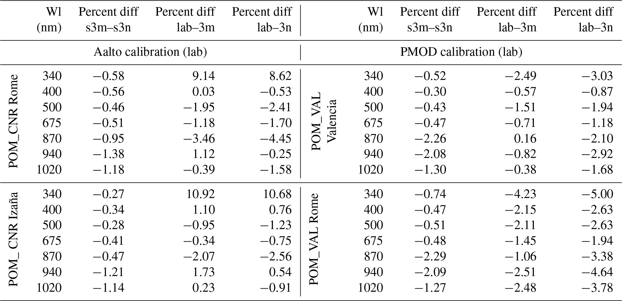
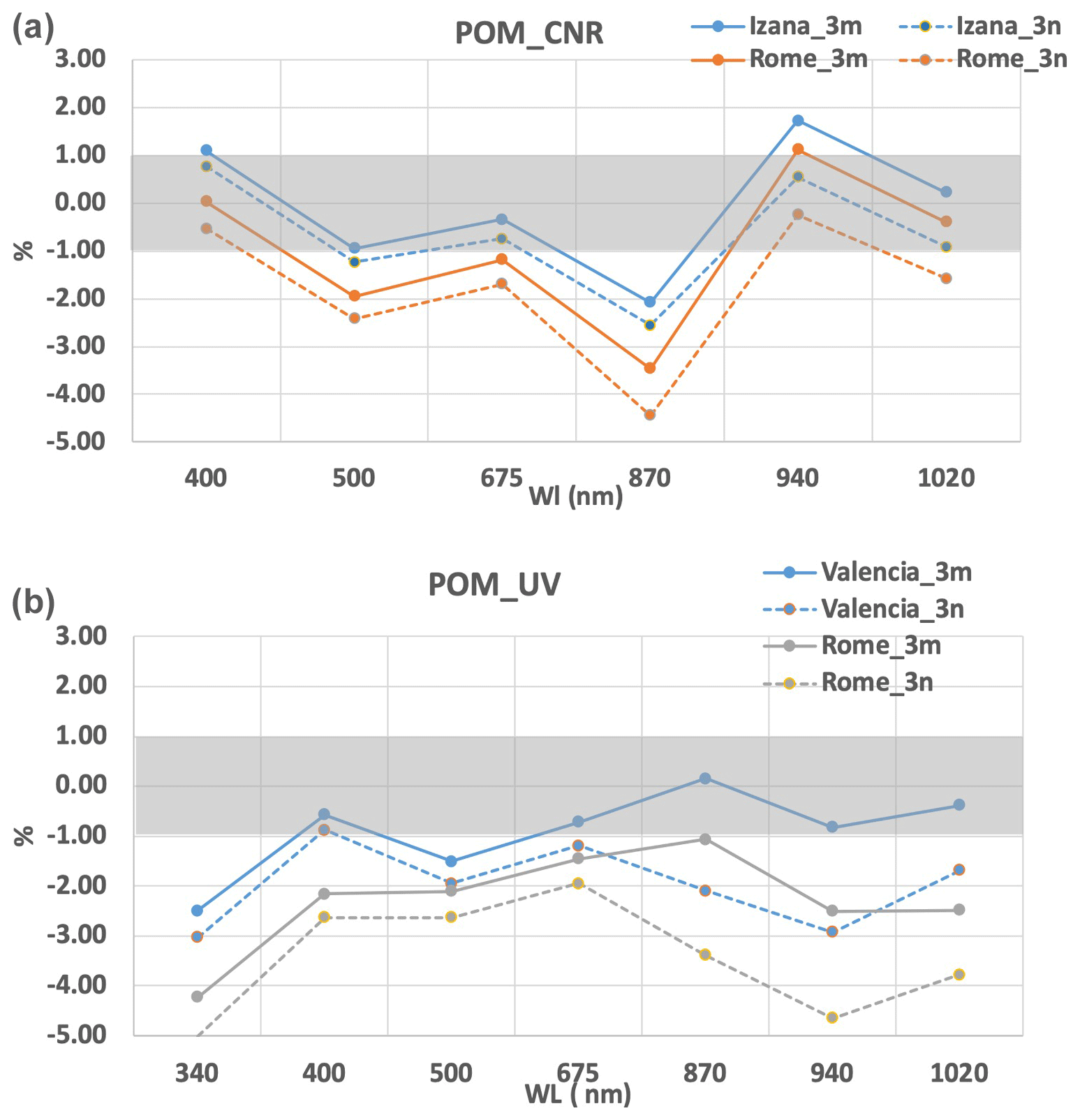
Figure 13 Percent difference of SVA values from sun disk methods and laboratory calibrations for POM_CNR (a) and POM_VAL (b).

The solar disk scanning matrixes, measured in Rome and Izaña and analyzed with the solid3m method, provide SVA values that generally agree better with the laboratory calibration than those obtained by the solid3n method. The difference varies from a minimum of 0.03 % at 400 nm to a maximum of 3.46 % at 870 nm in Rome and from 0.23 % at 1020 nm to 2.07 % at 870 nm in Izaña. Both methods slightly overestimate the SVA values in Rome. The 870 nm wavelength shows the highest discrepancy at both sites and for the solid3m and solid3n methods. At this moment we are not able to provide a reason for it, even if we expect it is due not to a physical cause but to an instrumental one. A general overestimation by the on-site procedures in the range of [500 nm, 870 nm] wavelengths is observed at both sites. The overestimation is explained considering that the field of view of a Prede POM is 1° and the size of the sun disk is about 0.5°; therefore, the scattered light from aerosols and air molecules is included in the measurement of the direct solar irradiance. Moreover, the direct solar light strikes the lens and results in stray light. The scattering contribution and stray light reaching the detector increase the output, and the integrated value has a larger magnitude that can affect the estimation of the SVA. The overestimation is lower in Izaña due to a less important scattering effect.

For POM_VAL, as for the other one, the 340 nm wavelength has a larger disagreement compared to the other wavelengths, reaching values of 4 % and 5 % for both sun disk methods, which is inexplicable at this stage. In both Rome and Valencia generally better agreement with the laboratory calibration is found for the solid3m method when in the range [400 nm, 870 nm] the difference is below 1.5 % and 2.15 % in Valencia and Rome, respectively. For the 1020 nm wavelength the comparison in Rome has a larger difference of up to 2.63 %. Also for this POM a general overestimation of SVA from on-site calibration is visible in Rome, as explained in the previous paragraph.

Finally, we compared the performance of the on-site calibration procedure, method solid3m, in Rome for the two co-located instruments calibrated at the two different laboratories (Fig. 14). The SVA values for POM_CNR better agree with the calibration performed in the Aalto laboratory, with the exception of 340 and 870 nm.

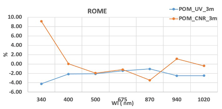
Figure 14 Difference of SVA values from the sun disk method solid3m and laboratory calibrations for POM_CNR (orange) and POM_VAL (blue) co-located in Rome.

5 Conclusions

The performance of the on-site calibration procedures applied to two Prede POM instruments was evaluated using intercomparison campaigns and laboratory calibrations. Two periods were chosen for the validation: (a) from September 2021 to November 2022, where six different calibration methodologies were compared against the SL performed in Izaña in September 2022 (the reference SL calibration was done in September 2022, and there is no availability of a monthly reference calibration in the previous 12 months, to watch the stability of the instruments and check if their shipments or usage affected the calibrations) and (b) from August 2017 to September 2021, where the calibration transfer from a PFR during the QUATRAM campaigns was used to evaluate the on-site methodologies.

The comparison against the SL showed very good agreement with many of the points within ±1 %. The IL works better in Davos with agreement below 0.5 % except at 1020 nm, where it increases by up to about 1.5 %. Very good agreement is also found in Valencia in November 2022 – always within 0.8 % except at 500 and 675 nm (within 1.5 %). The similarity between the two cases is probably due to the very low turbidity recorded in this month in Valencia, which makes the atmosphere optically more similar to the one in Davos. These results are in agreement with Nakajima et al. (2020), where the estimation of the retrieval accuracy of V₀ from IL gives values of about 2.4 % in Rome and around 0.3 %–0.5 % at the mountain sites of Mt. Saraswati and Davos. These values are consistent with the RMSD in the aerosol optical depth comparisons with other networks, which is less than 0.02 for λ ≥ 500 nm and about 0.03 for shorter wavelengths in city areas; smaller values of less than 0.01 are found in mountain comparisons.

The XIL provides a consistent improvement (with values within 1 %) only in Rome for all the wavelengths, but in a very clean atmosphere as in Davos it was not possible to retrieve values at 1020 nm.

The 340 nm wavelength is the one with the most problematic results for the on-site procedures in Rome (with differences of around 4 %), probably because of the molecular polarization that causes calibration errors from IL and XIL at 340 nm. The polarization effects become significant when AOD is low; therefore, they should be more evident in Davos, but they also depend on the surface pressure (in Davos lower than in Rome) and are therefore potentially weaker than in Rome.

In Rome the calibrations transferred from the PFR in September 2021 differ against the SL (performed in September 2022) in the range [−2.1 %, −1.9 %] at 500 nm for the two POM instruments, and the difference with the transfer from Cimel is about −1.6 %. However, simultaneous calculation of V₀ in September 2021 with IL and XIL at 500 nm provides values that differ from the SL by less than 0.5 % for POM_CNR and 1.2 % for POM_VAL. The reason for such a discrepancy must be studied, because is not attributable to a change in the equipment due to shipping or usage, since it would have been visible also from the on-site methodologies.

For both POM instruments the comparison with PTB laboratory calibration shows very high underestimations (down to −10 % for POM_CNR and −8 % for POM_VAL). The discrepancies between the laboratory-based values and the field measurements are probably due to different operating conditions of the instruments (e.g., different alignment and measurement geometries, operating modes, polarization) and unknown POM settings (e.g., POM temperatures, signal readout procedures) under which the instruments were calibrated in the laboratory and used in the field.

The long-term comparison of the on-site methods with the calibration transfer from the PFR was performed in Davos and Rome, and for IL it showed differences that were always greater than the uncertainties (%CV) of the method, for both wavelengths, with the exception of Davos in 2017. Values are around 1 % in Davos, whereas the largest differences are in Rome and at 500 nm, likely due to the unfulfilled assumption that the complex refractive index does not substantially change during the Langley plot.

On the other hand, for XIL many differences are within the uncertainties (%CV) of the method, and those higher are closer to the %CV values than in the IL method. XIL improves the agreement particularly in Rome, where the largest difference reduces from 3.5 % to 2.5 % at 500 nm and from 3 % to 1.7 % at 870 nm.

Future studies are planned to understand the effects of atmospheric scattering variability on the IL method and of the molecular polarization on 340 nm, switching from the use of the SKYRAD 4.2 pack to SKYRAD_MRI (Kudo et al., 2021).

The solar disk scanning methods solid3m and solid3n performed in Rome and Izaña were compared against the laboratory calibrations. The difference varied from a minimum of 0.03 % at 400 nm to a maximum of 3.46 % at 870 nm in Rome and from 0.23 % at 1020 nm to 2.07 % at 870 nm in Izaña. Both methods slightly overestimate the SVA values in Rome. The 870 nm wavelength shows the highest discrepancy at both sites and for the solid3m and solid3n methods for the two POM instruments. Generally better agreement with the laboratory calibration was found for the solim3m method. An overestimation by the on-site procedures in the range of [500 nm, 870 nm] wavelengths is observed at both sites, which is probably due to the effect of the scattered light from aerosols and air molecules included in the measurement and to a contribution of the direct solar light striking the lens. The scattering contribution and stray light reaching the detector increase the output, and the integrated value has a larger magnitude that can affect the estimation of the SVA. The overestimation was lower in Izaña due to a less important scattering effect.

Finally, the effects of the on-site calibration procedure uncertainties on the retrieval of aerosol optical depth, single-scattering albedo, and absorption aerosol optical depth will be investigated in an upcoming paper.

Appendix A: Abbreviations

ACTRIS	Aerosol, Clouds and Trace Gases Research Infrastructure
AM	Measured signal during solar disk scan
AOD	Aerosol optical depth
CIMO	Commission for Instruments and Methods of Observation
CV	Coefficient of variation
DN	Numbers of the digital signals
DUT	Detector under test
DVM	Digital voltage meter
ERR	Errors
FOV	Field of view
FRC	Filter radiometer comparison
FWHM	Full width at half maximum
GAW	Global Atmospheric Watch
$I/U$	Current-to-voltage converter
IL	Improved Langley method
LCD	Liquid crystal display
LSA	Laser spectrum analyzer

MAPP	Metrology for Aerosol optical Properties
MFRSR	Multi-Filter Rotating Shadowband Radiometer
MRI	Meteorological Research Institute
MUX	Multiplexer
NDF	Neutral-density filter
NIST	National Institute of Standards and Technology
OPO	Optical parametric oscillator
PFR	Precision filter radiometer
PMOD	Physikalisch-Meteorologisches Observatorium Davos
POM_CNR	POM01 sun–sky photometer of the Consiglio Nazionale delle Ricerche
POM_VAL	POM01 sun–sky photometer of the University of Valencia
POM_AM	POM01 sun–sky photometer of the Italian Air Force (Aeronautica Militare)
PTB	Physikalisch-Technische Bundesanstalt laboratory
QUATRAM	QUAlity and TRaceability of Atmospheric aerosol Measurements
REF	Reference
RMSD	Root mean square deviation
SHG	Second harmonic module
SL	Standard Langley method
SD	Standard deviation
SI	International System of Units
SSA	Single scattering albedo
SVA	Solid view angle
THG	Third harmonic module
TULIP	TUnable Lasers In Photometry
VIS	Visible
WMO	World Meteorological Organization
WORCC	World Optical Depth Research and Calibration Center
XIL	Cross-improved Langley method
ZM	Calculated signals during the fitting phase in the solar disk scan