Spatial analysis of PM_2.5 using a concentration similarity index applied to air quality sensor networks

Air quality sensor (AQS) networks are useful for mapping PM_2.5 (particles with a diameter of 2.5 µm or smaller) in urban environments, but quantitative assessment of the observed spatial and temporal variation is currently underdeveloped. This study introduces a new metric – the concentration similarity index (CSI) – to facilitate a quantitative and time-averaged comparison of the concentration–time profiles of PM_2.5 measured by each sensor within an air quality sensor network. Following development on a dataset with minimal unexplained variation and robust tests, the CSI function is used to represent an unbiased and fair depiction of the air quality variation within an area covered by a monitoring network. The measurement data is used to derive a CSI value for every combination of sensor pairs in the network, yielding valuable information on spatial variation in PM_2.5. This new method is applied to two separate AQS networks, in Dungarvan and in the city of Cork, Ireland. In Dungarvan there was a lower mean CSI value (${\stackrel{\mathrm{‾}}{x}}_{\text{CSI, Dungarvan}}=\mathrm{0.61}$, ${\stackrel{\mathrm{‾}}{x}}_{\text{CSI, Cork}}=\mathrm{0.71}$), indicating lower overall similarity between locations in the network. In both networks, the average diurnal plots for each sensor exhibit an evening peak in PM_2.5 concentration due to emissions from residential solid-fuel burning; however, there is considerable variation in the size of this peak. Clustering techniques applied to the CSI matrices identify two different location types in each network; locations in central or residential areas that experience more pollution from solid-fuel burning and locations on the edge of the urban areas that experience cleaner air. The difference in mean PM_2.5 between these two location types was 6 µg m⁻³ in Dungarvan and 2 µg m⁻³ in Cork. Furthermore, the examination of winter and summer months (January and May) indicates that higher PM_2.5 levels during periods of increased residential solid-fuel burning act as a major driver for greater differences (lower similarity indices) between locations in both networks, with differences in mean seasonal CSI values exceeding 0.25 and differences in mean seasonal PM_2.5 exceeding 7 µg m⁻³. These findings underscore the importance of including wintertime PM data in analyses, as the differences between locations is enhanced during periods when solid-fuel burning activities are at a peak. Additionally, the CSI method facilitates the assessment of the representativeness of the PM_2.5 measured at regulatory air quality monitoring locations with respect to population exposure, showing here that location type is more important than physical proximity in terms of similarity and spatial representativeness assessments. Applying the CSI in this manner can allow for the placement of monitoring infrastructure to be optimised. The results indicate that the population exposure to PM_2.5 in Dungarvan is moderately represented (${\stackrel{\mathrm{‾}}{x}}_{\text{CSI}}=\mathrm{0.63}$) by the current regulatory monitoring location, and the regulatory monitoring location assessed in Cork represented the city-wide PM_2.5 levels well (${\stackrel{\mathrm{‾}}{x}}_{\text{CSI}}=\mathrm{0.76}$).

1 Introduction

Air pollution affects the environment and quality of life and is a major cause of premature death and disease (Cesaroni et al., 2013; Lelieveld et al., 2015; Pedersen et al., 2013; Raaschou-Nielsen et al., 2013). The category of air pollutant with the largest impact on human mortality and health is fine particulate matter, i.e. atmospheric particles with an aerodynamic diameter of 2.5 µm or less (PM_2.5) (Pope et al., 2020; Pope and Dockery, 2012; Samoli et al., 2013). In many regions around the world, air quality monitoring and management have become critical endeavours to mitigate the detrimental effects of air pollution, and especially PM_2.5, on citizens and the environment.

Over the years, technological advances have provided valuable tools to enhance our understanding of air pollution, and low-cost air quality sensors (AQSs) are emerging as promising instruments for collecting real-time air quality data at an improved spatial and temporal resolutions (Kumar et al., 2015; Munir et al., 2019). When used in networks, air quality sensors offer immense potential for enhancing and supplementing regulatory monitoring and assessment (Malings et al., 2020). However, further work needs to be carried out to assess the effectiveness of sensor networks and how to make best use of the data for gaining further insights into air pollution within a locality because the data quality obtained with such low-cost devices does not meet the standards for regulatory monitoring. Careful consideration must be given to the quality of the data provided by sensors, and the requirement for calibration must be assessed (Diez et al., 2022). Recent studies have shown that the performance and calibration of a PM_2.5 sensor is dependent on the type of sensor and often on the measurement location, suggesting the need for site-specific and individual calibrations to correct for the absolute level of PM_2.5 (Kaur and Kelly, 2023; Sayahi et al., 2019; Wang et al., 2015; Zamora et al., 2020). When these factors are considered and accounted for, AQS networks offer an unprecedented opportunity to gain further insights into the complex dynamics of air pollution in localised areas, such as urban environments, industrial zones, and residential neighbourhoods (Crawford et al., 2021; Frederickson et al., 2022; Heimann et al., 2015; Hodoli et al., 2023; O'Regan et al., 2022).

Information on the spatial variation in air quality is important because air pollution is not homogenous and can exhibit significant variations across different areas even on a local scale (Frederickson et al., 2022, 2023; Kassomenos et al., 2014; Wang et al., 2018). The variability in air pollution can be influenced by a multitude of factors such as traffic patterns, industrial activities, meteorological conditions, and local topography. Consequently, relying on single monitoring locations or limited data resolution can provide an incomplete picture and inadequate understanding of local air quality in a certain area (Li et al., 2019). Understanding these variations is crucial for targeted interventions and policy decisions aimed at improving air quality and safeguarding public health. Spatial analysis facilitated by sensor networks allows for a more accurate and nuanced understanding of how air quality, and therefore exposure to pollution, varies across a population centre.

In a recent study, we used data collected by a PM_2.5 sensor network in the city of Cork, Ireland, to estimate the contribution of local pollution sources as separate and distinct from regional or transported air pollution (Byrne et al., 2023). The results highlighted the very localised nature of PM_2.5 caused by residential solid-fuel burning during winter, which is a significant problem in many towns and cities in Ireland and elsewhere (Dall'Osto et al., 2013; Kourtchev et al., 2011; Lin et al., 2018, 2019; Ovadnevaite et al., 2021; Wenger et al., 2020; Zhang et al., 2021).

In this work, we propose a new approach for assessing the spatial profile of air quality using an AQS network. The method yields a time-averaged concentration similarity index (CSI) for quantitative assessment of the similarity between the complete data series produced by different sensors within the network. The CSI is built on the premise that sensors exposed to similar ambient conditions and pollutant sources will produce comparable PM_2.5 temporal trends. Conversely, sensors subject to different conditions might display divergent PM_2.5 concentration trends. The motivation for the development of an assessment method based on the temporal variation over an extended period is the realisation that the annual average is often an incomplete representation of true population exposure, which is experienced from hour to hour and day to day. If hourly or daily PM_2.5 variability is high, it is not always adequate to merely compare annual averages of PM_2.5 in different locations to compare PM_2.5 exposure experienced by the local populations. While the annual average and hourly/daily values are often well correlated, numerous studies have found positive associations between short-term exposure to particulate matter and increased morbidity and mortality due to respiratory and cardiovascular diseases (Fajersztajn et al., 2017; Orellano et al., 2020; Weinmayr et al., 2010). This method aims to translate this idea into a quantifiable metric by calculating the time-averaged degree of similarity between two sensor datasets. After method development and testing, the CSI analysis is applied to an AQS network in the town of Dungarvan in Ireland to identify areas that may be experiencing persistently elevated or very localised PM_2.5 pollution compared to others. Clustering techniques are used to group sensors based on the similarity of their PM_2.5 measurements. The CSI method is also retrospectively applied to sensor network data collected in the city of Cork to investigate the transferability of the method between sensor networks and to explore any differences between the locations.

2 Methodology

2.1 Data collection, preprocessing, and calibration

The collection, preprocessing, and calibration of the data collected by the PM_2.5 sensor networks in Dungarvan and the city of Cork were carried out using the Julia programming language and the openair package written for the R programming language (Bezanson et al., 2017; Carslaw and Ropkins, 2012). Since low-cost AQSs are not of regulatory standard, great care needs to be taken with quality assessment and quality control of the data. In particular, the degree to which changes or differences in PM_2.5 measurements between devices can be trusted needs to be considered. The methodology proposed here addresses these inherent issues to deliver an approach for assessing the spatial representativeness of any monitoring location and to facilitate comparison of different environment types, regardless of geographical distance to the location.

2.1.1 Dungarvan PM_2.5 sensor network

The Dungarvan sensor network consisted of 18 solar powered Clarity Node-S devices (Clarity Movement Co., USA), which utilise the Plantower PM6003 sensor to measure PM_2.5 within the range of 1–1000 µg m⁻³ and at a resolution of 1 µg m⁻³ (Clarity Movement Co., 2023; Node-S technical sheet, 2023). By default, the Node-S devices take measurements every 15 min, allowing sufficient data upload and battery sleep time in between sampling periods. However, this can be adjusted to higher or lower frequencies. The highest sampling interval achievable during winter without significantly affecting the battery performance was 8 min.

The Clarity Node-S devices were typically attached to street light poles between 2 and 4 m above the ground. The sensors were positioned in a range of different environments including urban background, residential, coastal, and roadside locations (Fig. S1 in the Supplement). Many of these locations were a mix of the different environments. The majority of devices were operational from 1 November 2022 to 31 May 2023; however three devices (AP7, AY9N, AY93) with the Clarity Wind Module were only deployed from 12 January 2023. Measurements were taken over a continuous period covering different meteorological seasons (mainly winter and spring/early summer), thus ensuring that temporal variations in PM_2.5 concentrations were captured comprehensively.

Prior to and after deployment in Dungarvan, the Clarity Node-S devices were co-located on the roof of the Ellen Hutchins Building, University College Cork (51.895136, −8.516146), to compare their performance. Details of the three co-location periods are outlined in Table S1 in the Supplement. Although some devices were not available for all three co-location periods, the three periods combined provide a comparison between the sensors across different seasons. This co-location dataset enabled the CSI method to be developed on measurements that in theory should be equal, and the function could then be modified if necessary to allow for sensor behaviour, uncertainties, errors, and potential limitations.

The raw sensor data from the co-location periods and field deployment underwent a series of preprocessing steps to mitigate potential sources of error in the measurement and to ensure data quality and consistency. Data points outside of the operational range of the sensors (>1000 µg m⁻³) were identified and removed, although instances of these were minimal. The 8 min data were averaged to produce hourly measurements. Missing data points could potentially affect the temporal continuity of the data; however, the data coverage was overall very good for the co-location and measurement campaign periods. On average, the devices had an hourly measurement coverage of 87 % for the field measurement campaign. This corresponds to an average of 4443 hourly measurements per device for the campaign period.

Assessing the consistency of measurements across the sensor network was paramount. Although the PM_2.5 readings were very well correlated when the devices were co-located (Table S2 in the Supplement), a data harmonisation procedure was performed to ensure the uniformity of sensor measurements, which is a prerequisite for the subsequent development of the concentration similarity index. Since there was no reference-grade PM_2.5 data available during the co-location periods, the PM_2.5 concentrations from each sensor were scaled to a common reference point, represented by the mean of all data points across the whole co-location dataset (Fig. S2 in the Supplement). The data series for each sensor was then individually compared with the calculated mean dataset and subsequently harmonised to the common reference point using a simple linear regression approach. The equations resulting from this harmonisation procedure were applied to the measurements collected from all devices during the subsequent field measurement campaign. While this procedure did not convert the measured PM_2.5 to reference-equivalent concentrations, it minimised sensor output variability and facilitated a more equitable comparison between sensor measurements (Table S2).

2.1.2 Cork PM_2.5 sensor network

For brevity when referring to the sensor network, the term “Cork” will herein refer exclusively to the city area of Cork. The Cork sensor network consisted of 16 PurpleAir PA-II-SD units that each contain two Plantower PMS5003 sensors to measure PM_2.5 within the effective range of 0–500 µg m⁻³, with a maximum range of 1000 µg m⁻³, and at a resolution of 1 µg m⁻³ (PMS5003 series data manual, 2022). In this study, data recorded by the devices in the network for the periods from 1 January 2021 to 31 May 2021 and from 1 September 2021 to 31 December 2021 were collated and analysed. However, four devices were found to have limited data capture for the specified periods (<50 %) and were therefore omitted from the analysis. The 12 sensors used in this analysis had an average data capture of 85 % for the specified periods; their locations are shown in Fig. S3 in the Supplement.

Due to logistical constraints, it was not possible to co-locate all of the PurpleAir devices together to assess variability in PM_2.5 concentrations. However, low inter-sensor and inter-unit variability was exhibited by four co-located PurpleAir devices in our previous study on the Cork network, where all inter-sensor and inter-unit comparisons yielded R² values greater than 0.98 (Byrne et al., 2023). Moreover, PurpleAir PM_2.5 measurements were highly correlated (R²=0.92) with hourly values of PM_2.5 concentrations obtained using a Met-One (USA) beta-attenuation monitor (BAM-1020). The comparison yielded a low offset (0.3 µg m⁻³), although reference measurements tended to be lower than the sensor measurements (slope=0.57). A co-location dataset was then used to derive calibration factors incorporating the effects of temperature and relative humidity. The data processing procedures for obtaining the PM_2.5 concentrations reported here are identical to those reported by Byrne et al. (2023).

The Cork dataset spans a similar measurement period to the Dungarvan dataset to allow for comparable results due to the known seasonality of PM_2.5 pollution in Ireland (Ovadnevaite et al., 2021). Although the year 2021 included some periods of COVID-19 pandemic restrictions, such measures mainly affected NO₂ concentrations and were not shown to have a significant impact on PM levels in Ireland (Environmental Protection Agency, EPA, 2020).

2.1.3 Meteorological measurements

Meteorological data was analysed in each location. For the city of Cork, data collected at Cork Airport by Ireland's National Meteorological Service, Met Éireann, was accessed from the website https://www.met.ie (last access: 25 April 2024). The airport weather station is located approximately 5.5 km from the Cork city centre.

There is no weather station located nearby Dungarvan that provides hourly measurements; however three of the Clarity Node-S devices were fitted with Clarity Wind Modules (AP7, AY93, AY9N), which provide high-time-resolution measurements of wind speed and direction (Clarity Movement Co., USA). Due to technical difficulties, device AY9N did not capture wind direction measurements, however its wind speed is included. The Wind Module contains a solid-state two-axis ultrasonic anemometer, which provides wind speed measurements with a range of 0–60.00 m s⁻¹ and a resolution of 0.01 m s⁻¹, along with wind direction at a resolution of 0.1° over a range of 0–359.9° (Wind Module technical sheet, 2024). These measurements have not been validated against reference meteorological data; however, they are included for indicative purposes.

2.2 Development of the concentration similarity index

The concentration similarity index (CSI) derived here quantifies the degree of likeness between PM_2.5 concentration profiles from two sensors for a defined period of time and forms the basis for assessing the spatial disparities in PM_2.5 measurements within sensor networks. The methodology proposed was developed through multiple iterations in order to adjust and improve the procedure. An overview of the development is described, showing the evolution towards the final method.

2.2.1 Original function application

The first phase of development was based directly on the work carried out by Piersanti et al. (2015), who used a concentration similarity function to assess the spatial representativeness of PM_2.5 and O₃ monitoring stations in the Italian air quality monitoring network. Using modelled hourly air pollutant data covering Italy with a 4 km×4 km grid cell resolution, Piersanti et al. (2015) produced maps showing how representative certain sites in the Italian monitoring infrastructure were. The application proposed here compares point measurement to point measurement as opposed to comparing modelled grid cell data; however, the underlying principle of comparing two concentration–time profiles to produce a single indication of similarity between them still applies. The function value f_site(x,y) used by Piersanti et al. (2015) to assess the spatial coverage of point measurements is given in Eq. (1):

$$\begin{array}{}\text{(1)}& f_{\text{site}}(x,y)={\displaystyle \frac{{\sum }_{i=\mathrm{1}}^{N_t}\text{flag}}{N_t}},\end{array}$$

where

$$\text{flag}=\left\{\begin{array}{ll}\mathrm{1},& \frac{\left|C\right(X_{\text{site}},Y_{\text{site}},t_i)-C(x,y,t_i\left)\right|}{C(X_{\text{site}},Y_{\text{site}},t_i)}<\mathrm{0.2}\\ \mathrm{0},& \frac{\left|C\right(X_{\text{site}},Y_{\text{site}},t_i)-C(x,y,t_i\left)\right|}{C(X_{\text{site}},Y_{\text{site}},t_i)}>\mathrm{0.2},\end{array}\right.$$

and where $C(x,y,t_i)$ represents the surface concentration from the modelled data in a grid point at time t_i, $C(X_{\text{site}},Y_{\text{site}},t_i)$ represents the modelled data of a specific site of interest at time t_i, and N_t is the total number of time steps. The study defined a modelled grid cell at the site of interest as representative of a surrounding grid cell area if the condition $f_{\text{site}}(x,y)>\mathrm{0.9}$ is true.

In the first step of our approach, this function was applied to the hourly average PM_2.5 data obtained from the co-located Clarity Node-S units by comparing two sensor data series at a time. The concentration at the point of interest and surrounding grid cell concentration inputs were substituted for sensor PM concentration values from any given sensor A and sensor B pair, C(A,t_i) and C(B,t_i). Over a total of 1565 co-located hours, the mean number of comparable data points per C(A,t_i), C(B,t_i) pair was 654 due to devices being present at different stages during the co-location periods (Table S1).

Table 1 Function values, f_site(x,y), for hourly averaged PM_2.5 measured by a range of co-located Clarity Node-S devices. Device labels in the columns were set as $C(X_{\text{site}},Y_{\text{site}},t)$, and device labels in the rows were set as $C(x,y,t_i)$.

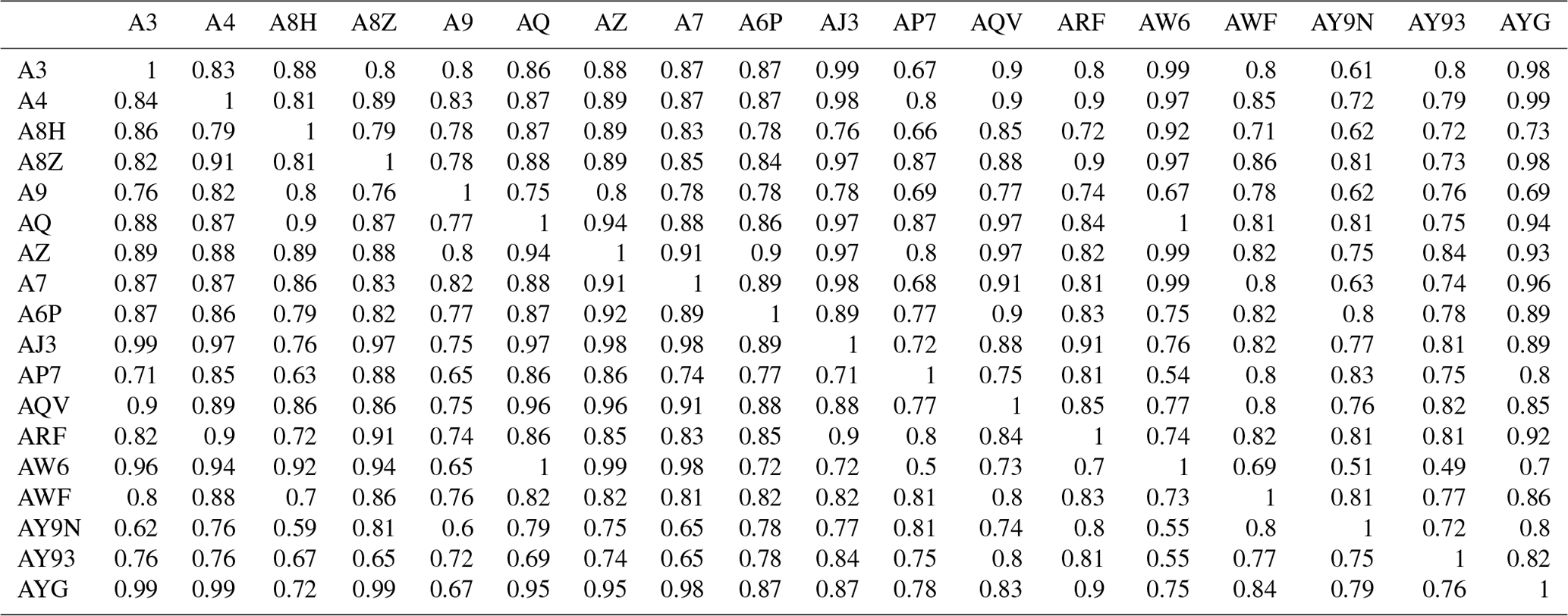
In theory, the function value comparing two sensor data series would be 1, given that the measurements were collected in the same location and were known to all represent the same air parcel at each point in time. However, it was found that the function was not comprehensive enough to allow for an acceptable comparison of the sensor data. The results showed discrepancies between some device pairs because the function value deviated significantly from 1 in many cases (Table 1) and was as low as 0.51 in some cases, with an overall mean of 0.82.

2.2.2 Function parameter optimisation and introduction of PM limit

Analysis of the results obtained from direct application of the original function showed that the conditions set out by it were too strict to apply to the sensor data, given the variations that can occur in AQS measurements. The areas of the entire sensor networks discussed here could be within the original single grid cell size analysed by Piersanti et al. (2015). Therefore, overall pollution dynamics would vary significantly, in part because of hyper-local effects, and pollution averaging effects would be more pronounced when assessing larger areas. Moreover, the high hourly PM_2.5 variation and very localised effects exhibited in a typical Irish winter PM_2.5 profile are not suited to the original function (Byrne et al., 2023). While the original application contains a mathematical function examining the difference between two pollutant concentrations and is independent of specifications regarding area size and pollution dynamics, the threshold values can be adapted to reflect the specific application of the function. A second threshold value, a PM mass concentration limit, PM_lim, was introduced to the function, with different relative concentration limits for the upper and lower PM values, C_{lim, upper} and C_{lim, lower}, respectively. Treating larger and smaller PM_2.5 values differently when assessing the similarity between two data series is useful for capturing the nuanced relationships and patterns in the data. It allows for the real-world significance of the data to be reflected, acknowledging the varying implications of PM_2.5 measurements based on the magnitude. Higher PM_2.5 values can indicate a pollution episode or specific local pollution sources, while lower values can represent background levels. Therefore, treating lower PM_2.5 values with more leniency in the similarity assessment recognises that minor fluctuations in low hourly concentrations might not be as concerning as similar deviations in higher concentrations and the health-related considerations associated with these high concentrations.

Another potential advantage of the PM limit concerns the varying degrees of accuracy of the AQS measurements. Allowing the leeway introduced here in assessing the similarity of lesser measurement values considers potential measurement uncertainties with these devices. However, it is important to note that this approach is not accommodating sensor limitations at the expense of accuracy, but rather it is a strategy to ensure that the assessment remains faithful to the underlying air quality dynamics while accounting for the potential deficiencies in measurement equipment.

When the function is applied to a pair of sensors, the resulting CSI can differ slightly depending on which sensor was classified as $C(x,y,t_i)$ or $C(X_{\text{site}},Y_{\text{site}},t_i)$, or sensor A or sensor B, in Eq. (1) when computing the difference at each time step. Due to the nature of the function, the denominator value of the relative difference calculation, the concentration of sensor A at a given time step, is what makes the difference. To counteract this and to avoid the possibility of large discrepancies between the CSI values for a sensor pair depending on which sensor is taken as A or B, the function was modified to use the geometric mean, or the square root of the product, of C(A,t_i) and C(B,t_i) as the denominator. This ensured symmetry in the function so that the CSI values were identical regardless of which sensor was classified as A or B in a sensor pair.

Equation (2) shows the next form of the concentration similarity function (function notation has been modified to be more suitable for this application).

$$\begin{array}{}\text{(2)}& {\text{CSI}}_{A,B}={\displaystyle \frac{{\sum }_{i=\mathrm{1}}^{N_t}f}{N_t}},\end{array}$$

where

$$f=\left\{\begin{array}{ll}\mathrm{1}& \text{if}\frac{\left|C\right(B,t_i)-C(A,t_i\left)\right|}{\sqrt{C(A,t_i)\times C(B,t_i)}}<C_{\text{lim, upper}}\\ & \text{and}C(A,t_i)\text{or}C(B,t_i)>{\text{PM}}_{\text{lim}}\\ \mathrm{0}& \text{if}\frac{\left|C\right(B,t_i)-C(A,t_i\left)\right|}{\sqrt{C(A,t_i)\times C(B,t_i)}}>C_{\text{lim, upper}}\\ & \text{and}C(A,t_i)\text{or}C(B,t_i)>{\text{PM}}_{\text{lim}}\\ \mathrm{1}& \text{if}\frac{\left|C\right(B,t_i)-C(A,t_i\left)\right|}{\sqrt{C(A,t_i)\times C(B,t_i)}}<C_{\text{lim, lower}}\\ & \text{and}C(A,t_i)\text{or}C(B,t_i)<{\text{PM}}_{\text{lim}}\\ \mathrm{0}& \text{if}\frac{\left|C\right(B,t_i)-C(A,t_i\left)\right|}{\sqrt{C(A,t_i)\times C(B,t_i)}}>C_{\text{lim, lower}}\\ & \text{and}C(A,t_i)\text{or}C(B,t_i)<{\text{PM}}_{\text{lim}},\end{array}\right.$$

and where C(A,t_i) and C(B,t_i) are the PM_2.5 measurements from devices A and B at time, t_i. C_{lim, lower} and C_{lim, upper} are the threshold values defining the acceptable level of difference between two concentrations, and PM_lim is the PM mass concentration threshold value.

2.2.3 Development and testing of the modified equation

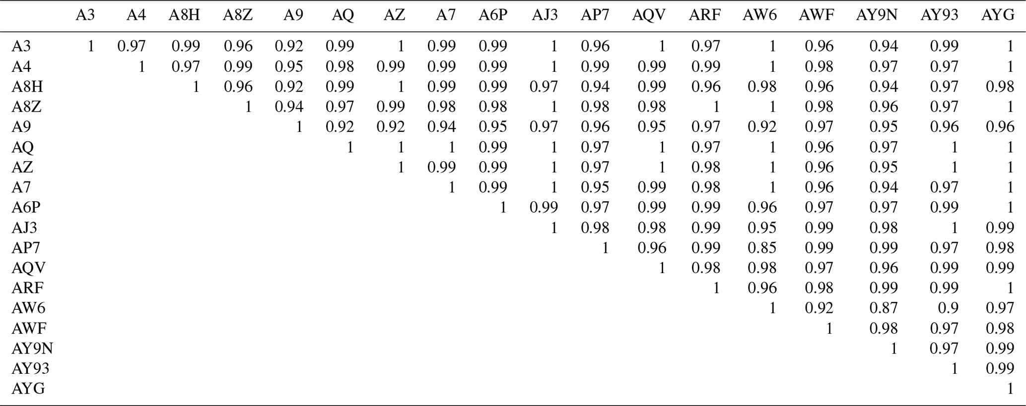
The PM limit and associated concentration similarity limits introduced were chosen by iteratively testing the similarity function on the co-location data using different limits. Each co-located sensor pair was tested with different PM_lim values (5, 10, 15, 20 µg m⁻³) and with C_lim values ranging from 0.1 to 2.0 in steps of 0.1 for both the upper and lower limits. This produced a C_lim vs. CSI comparison for each A–B pair for data above and below the corresponding PM_lim value. The C_lim value for each sensor comparison, which gave a minimum CSI value of 0.95, was recorded with the overall mean of these C_lim values above and below each PM_lim value taken forward. The mean C_lim pair values were then applied to the co-location measurements with the respective PM_lim values to give final CSI values for each sensor pair, highlighting how the PM_2.5 concentration profile of each sensor compares to that of all the other sensors. The highest mean CSI value for all co-located A–B pairs was found for PM_lim=15 µg m⁻³, C_{lim, upper}=0.2, and C_{lim, lower}=0.7. When applying these new limits, all sensor pairs gave CSI>0.85, with 99 % of pairs above 0.90 and with an overall CSI mean of 0.98. These final limits enabled a good comparison for the hourly co-located AQS measurements (Table 2).

Table 2 Concentration similarity indices for hourly averaged PM_2.5 measured by a range of co-located Clarity Node-S devices. PM_lim=15 µg m⁻³, C_{lim, upper}=0.2, and C_{lim, lower}=0.7.

The CSI function was also applied to data obtained from the four co-located PurpleAir devices in order to make sure that the function was applicable across the two AQS types. The data was harmonised by following the same procedure as the Clarity device data, through scaling each data point from each sensor to the mean data series of all four sensors. Although this co-location period was shorter than that of the Clarity dataset used for the function development, it still allowed for the CSI to be calculated from around 250 common data points per sensor pair. All device pairs reported a CSI close to 1.0, with a mean CSI of 0.99 (Table S3 in the Supplement).

The function described in Eq. (2) was further tested by comparing the sensors to numerous sets of synthetic data created from each sensor's measurements to assess the impact of a range of scenarios. Comparing a sensor dataset to itself establishes a baseline for the comparison where the CSI is 1 and any subsequent adjustments to the data to create the synthetic data can be explored, resulting in a new CSI. The first scenario investigated changes in CSI when outliers are present in the data. To explore this, the sensor data was changed so a certain number of data points could be considered outliers (n=1, 10, 500, 1000). An outlier data point was created by increasing a value by 100 µg m⁻³ in order to ensure discrepancy between it and the original value. The function was then tested in a scenario where the data was scaled linearly so the mean remained constant, but the variance of the data was increased, and it was also tested in a scenario where the entire dataset was offset by 5, 10, 15, and 20 µg m⁻³. The final test scenario involved the introduction of noise to the dataset, representing impactful variations in that data. Gaussian noise with various values of standard deviation was added to the data. The CSI results for the synthetic data tests were also compared to the results when the R² was found between any two given datasets. Low variations were found during all synthetic data analyses, with the resulting CSI values having standard deviations ≤0.05 across the individual devices for each test. As an example, the effects of these tests on the CSI results for A6P are shown in Table 3, where 4406 data points were included in the calculations.

Table 3 Influence of data outliers and other factors on CSI determined in test scenarios with device A6P.

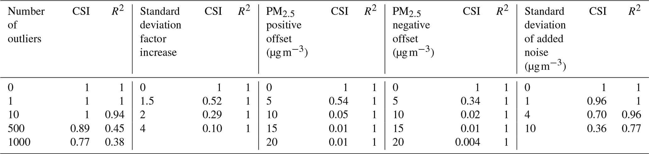
It is clear that in the case of the linearly scaled data with higher variability but the same overall mean, the CSI is impacted (CSI=0.52) when the standard deviation is increased by just a factor of 1.5, indicating that such a dataset is dissimilar to the original. In comparison, the R² is not an accurate reflection of the change, as it does not deviate from 1. Offsetting the data by different degrees also shows a major change in the CSI (CSI<0.55). However, this is not reflected well in the R² values, which do not deviate from 1. The CSI method is quite robust with respect to outliers, whereas the R² is more sensitive (R²=0.94) when 10 outliers are introduced to the dataset, which is approximately 0.2 % of the total data points. The R² is significantly reduced (R²=0.45) with 500 outliers (∼11 % of the total data points), whereas the CSI is only slightly impacted (CSI=0.89). As the method yields a time-averaged result, low numbers of outliers do not hugely affect the index for a given sensor pair. So, two datasets that are generally similar but where one experiences some outliers will be deemed similar by the method. The R² also shows a more limited response when larger amounts of Gaussian noise are added, resulting in a value of 0.96 when the standard deviation of the noise is 4 µg m⁻³, while the CSI is adjusted to 0.7. From a health-impact and exposure point of view, increased variation and higher offset represent very different exposure scenarios, whereas a large difference in the occasional hourly average in an otherwise similar exposure regime does not. The CSI offers a more appropriate comparison between hourly measurements collected at two locations.

2.3 Application to sensor networks and analysis of spatial trends

The CSI methodology developed above was subsequently applied to the Dungarvan and Cork sensor networks to evaluate the similarity and spatial variations in PM_2.5. A systematic pairwise comparison approach was employed, wherein each sensor was individually compared to every other sensor within the network. Hierarchical clustering and fuzzy c-means (FCM) clustering were both performed on the CSI results to identify groupings based on each sensor's relationship to other sensors in the network that can then be reflected spatially.

With both clustering techniques, the quality of cluster assignments can be assessed with various evaluation metrics to choose the optimal number of clusters. As the “true” cluster classifications are not known here, validation must be performed using the clustering algorithm itself. To assess the quality of the hierarchical clustering assignments, the silhouette metric was used along with the Calinski–Harabasz index to assess the FCM assignments (Caliński and Harabasz, 1974; Rousseeuw, 1987). The silhouette score, ranging from −1 to +1, can be calculated for each member of a cluster and then the mean silhouette score from all members indicates an overall assignment quality for members of that cluster, with a high score closer to 1 indicating higher-quality clusters and a low or negative score indicating poorer cluster assignments. The Calinski–Harabasz index also quantifies the quality of cluster assignments, with higher scores indicating better quality. The metrics were used to test for the optimal number of clusters for each algorithm.

3 Results and discussion

3.1 Dungarvan PM_2.5 sensor network

Analysis of the harmonised data obtained from the sensors in the Dungarvan PM_2.5 network was conducted to determine CSI values and assess the spatial variation in air pollution across the town. Although the PM_2.5 concentrations are not as accurate as those collected by reference instrumentation, any relative differences between the sensors and between individual sensor data trends can be regarded as genuine due to the low inter-sensor variation observed after data harmonisation procedures, where the standard deviation of the mean PM_2.5 co-located measurements was 1.7 µg m⁻³.

The temporal and spatial trends of PM_2.5 across the Dungarvan sensor network are reflected in the average diurnal plots obtained for each sensor, Fig. 1. These diurnal profiles all show large evening peaks in PM_2.5, which are typical of towns and cities in Ireland affected by residential solid-fuel burning during winter evenings (Dall'Osto et al., 2014; Healy et al., 2010; Wenger et al., 2020). However, there are clear disparities in some of the average evening peak values between the sensors. One group of sensors has maximum values above 35 µg m⁻³ (A3, A4, A8H, A9, AQ, A7, AW6, AQV), while the sensors with maxima below 35 µg m⁻³ can be further divided into three smaller groups. Sensors labelled AJ3, AWF, and AZ all have a maximum PM_2.5 concentration around 30 µg m⁻³; sensors AY9N, AY93, ARF, A8Z, AYG, and A6P all have maxima in the 20–26 µg m⁻³ range, while AP7 has a significantly lower evening peak than all other devices.

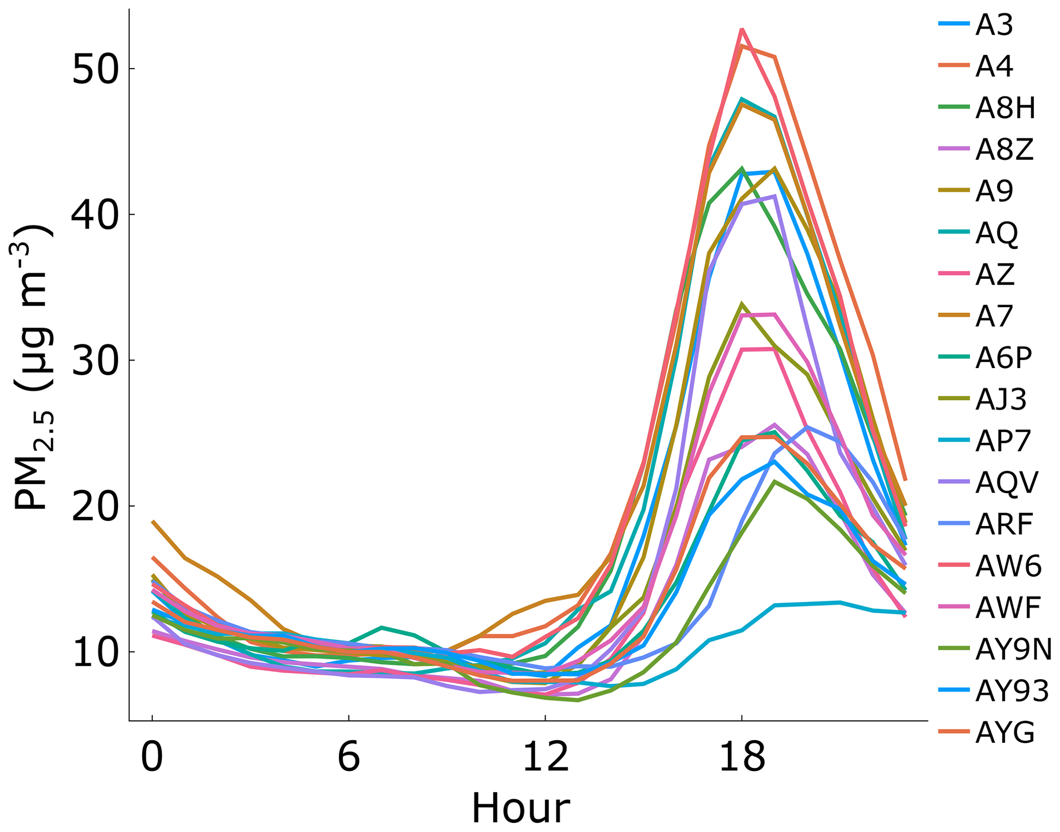
Figure 1 Diurnal profiles for hourly averaged measurements of PM_2.5 in the Dungarvan sensor network (September 2022 to May 2023).

Most sensors exhibited the diurnal maximum around the same time of day, between 18:00 and 20:00 LT; however AP7 and ARF showed a slightly delayed peak from 20:00 to 22:00 LT. AP7 had the lowest peak concentration and did not exhibit the sharp rise and subsequent decrease associated with evening solid-fuel burning that the other sensors showed. AP7 was located on the southwestern edge of the town, and since the predominant wind direction is southwesterly, it did not measure as much local pollution as other locations in the eastern part of the network.

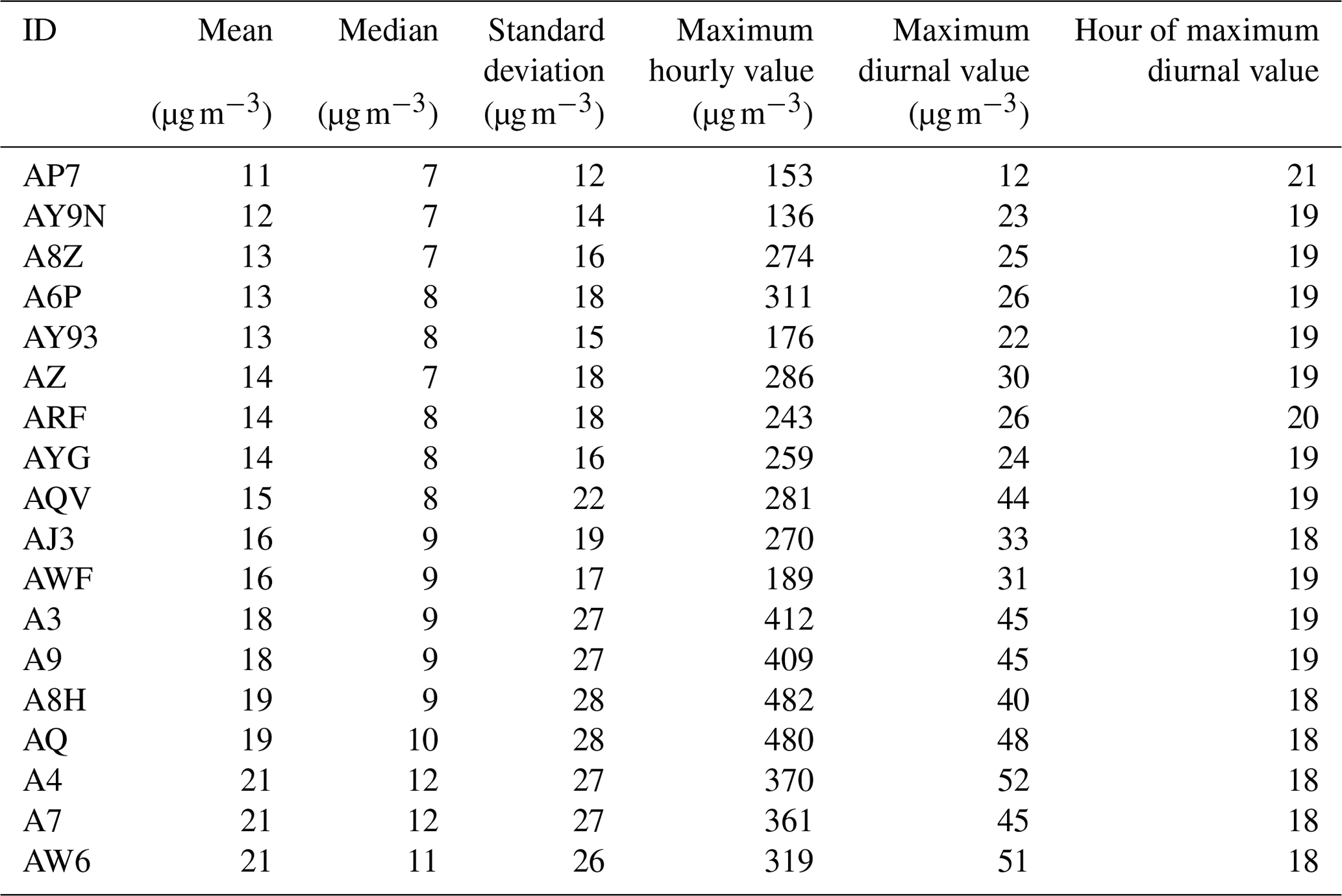
Summary statistics obtained for the 18 sensors in the Dungarvan network are listed in Table 4. Unsurprisingly, most of the devices with diurnal maxima >35 µg m⁻³ have the highest mean, median, and maximum values. Out of this subset of devices, AQV has the lowest overall mean (15 µg m⁻³) but still has a relatively high standard deviation (22 µg m⁻³), indicating that the PM_2.5 values tend to vary widely but are lower on average. This could be indicative of fluctuating particle concentrations, consistent with intermittent pollution sources such as residential solid-fuel burning.

Table 4 Summary statistics of hourly average PM_2.5 concentrations obtained for all sensors in the Dungarvan sensor network (September 2022 to May 2023).

The wind speed and direction recorded at sites AP7 and AY93 showed some variation (Fig. S4a and b in the Supplement); however, wind speeds measured at all three sites showed a moderate correlation with all R² values above 0.65. The measured wind direction at the AP7 and AY93 sites reported a moderate correlation (R²=0.63). Both sites measured winds emanating from a broad range of directions. Both locations reported generally southerly winds 53 % of the time and southwesterly winds 30 % of the time. The temporal variations in wind speed measured at the three sites are detailed in Fig. S5 in the Supplement. Little diurnal variation is seen between devices AY93 and AY9N; however, it is clear that AP7 tended to experience slightly lower wind speeds than AY93 and AY9N during the measurement campaign. Nevertheless, this difference did not exceed 1 m s⁻¹ in any of the temporal variation assessments, and all three sites reported the same overall trends in wind speed. The variations in wind measurements between the sites indicate some slight local meteorological differences; however, the overall meteorological field is not likely to differ greatly between the three sites.

3.1.1 Concentration similarity index

The matrix of CSI values obtained for the Dungarvan sensor network is shown in Table 5. The results can be analysed in a number of ways. Firstly, the indices for one sensor can be used to assess how similar or dissimilar the measurements are to all other sensors in the network, thus providing information on the spatial representativeness of that particular location. Secondly, the indices of all sensors can be looked at together to elucidate any potential relationship between sensor measurement locations.

Table 5 Concentration similarity indices for the hourly averaged PM_2.5 concentrations measured by Clarity Node-S devices in the Dungarvan sensor network.

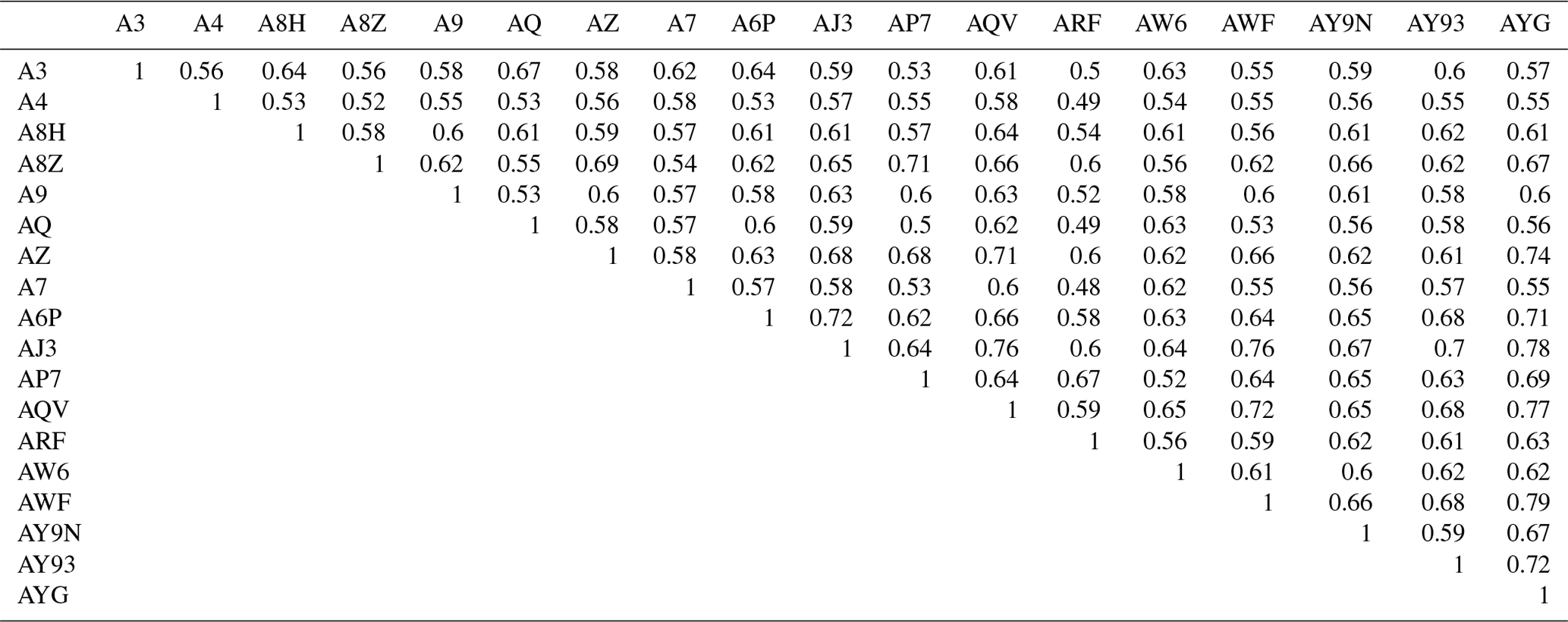
The minimum CSI value (0.85) determined during the co-location deployment can act as the lower limit for when two sensor locations can be considered very similar. The reported CSI values for Dungarvan sensors ranged from 0.48 (ARF vs. A7) to 0.79 (AYG vs. AWF) with a mean of 0.61, indicating a significant difference in air quality representation between locations across the town. The device with the lowest mean of its CSI values with respect to the other locations was A4 (0.55), and although device ARF was only slightly above this (0.57), it reported a larger range of CSI values, including the lowest of the entire dataset. AJ3, AQV, and AYG all shared the highest mean CSI values (0.66).

To further investigate the effect of solid-fuel burning on local air quality, the CSI function was applied to data from two isolated months – January and May 2023. The purpose of this assessment was to evaluate the extent to which residential solid-fuel burning dictates the CSI between two sensors, given that one month (January) will have higher PM_2.5 levels, with measurements heavily influenced by solid-fuel burning, and the other will not (May). For both months, all sensors had data capture above 65 %, and the mean capture was 94 % for January and 92 % for May. The January mean CSI from all comparisons was 0.51, and the May mean CSI was 0.84 (Tables S4 and S5 in the Supplement). The large discrepancy between the mean CSI for January and May is most likely due to the higher variation typically seen in wintertime PM_2.5 (s_January=25 µg m⁻³, s_May=9 µg m⁻³) due to residential solid-fuel burning (Fig. 1). This highlights the importance of seasonality when assessing the spatial representativeness of monitoring network locations.

3.1.2 Clustering

Clustering techniques were employed on the CSI matrix to uncover any inherent spatial relationships between different locations in the network. Hierarchical clustering produced a dendrogram showing the hierarchical relationship between the sensor locations and was used to identify clusters (Fig. 2). The highest mean silhouette score was found with two clusters (Fig. S6 in the Supplement). However, it was not a high silhouette score (0.19), indicating that the quality of the cluster assignments was low. The highest Calinski–Harabasz index corresponded to the assignment of members to two clusters when applying the FCM clustering (Fig. S7 in the Supplement).

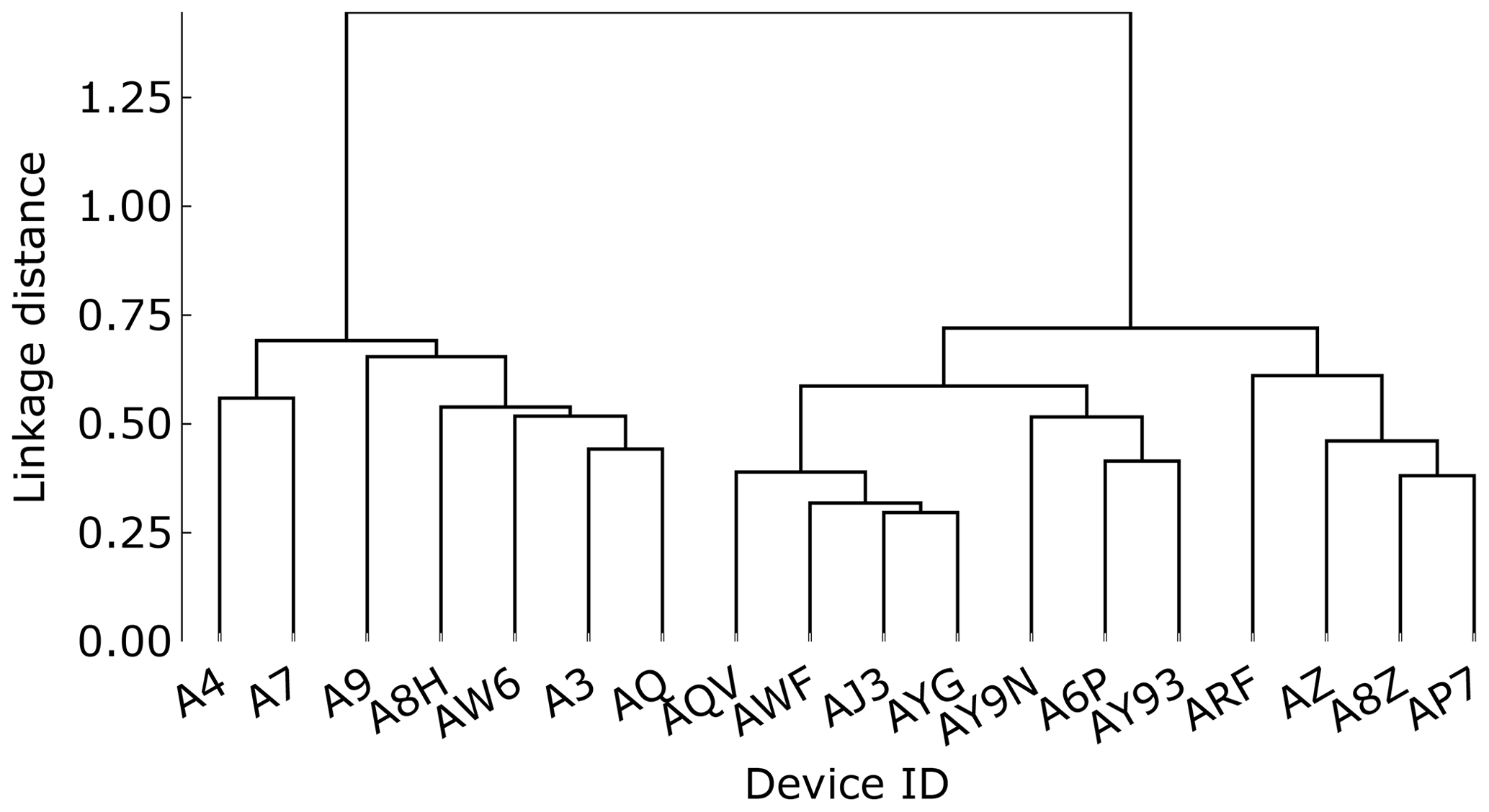
Figure 2 Dendrogram output from hierarchical clustering of the CSI data from the Dungarvan sensor network.

From both the dendrogram (Fig. 2) and the FCM membership weights (Fig. 3), it is clear that devices A4 through AQ are grouped together in one cluster (Cluster 1), and devices AQV to AP7 are grouped in another cluster (Cluster 2). This split is very similar to the easily visualised groupings shown in the diurnal profile maxima (Fig. 1), with the only difference being device AQV. The devices in Cluster 1 are also those with the highest mean PM_2.5 for the measurement period. The mean CSI for each sensor mostly corresponds to the cluster assignments, with Cluster 1 devices having a mean CSI equal to or below 0.6 and all devices in Cluster 2 having a mean CSI above 0.6 except for device ARF. Interestingly, this grouping also appears to have spatial importance too, as shown in Fig. 4. Cluster 2 devices are mainly located around the edge of the town and generally experience cleaner air (${\stackrel{\mathrm{‾}}{x}}_{\text{PM2.5}}=\mathrm{13}$ µg m⁻³, s_PM2.5=27 µg m⁻³), while Cluster 1 devices are located in central and residential areas (${\stackrel{\mathrm{‾}}{x}}_{\text{PM2.5}}=\mathrm{19}$ µg m⁻³, s_PM2.5=17 µg m⁻³), which are more polluted during winter months.

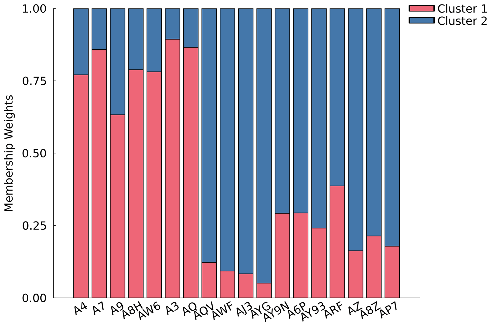
Figure 3 Membership weights from FCM clustering of the CSI data from the Dungarvan sensor network.

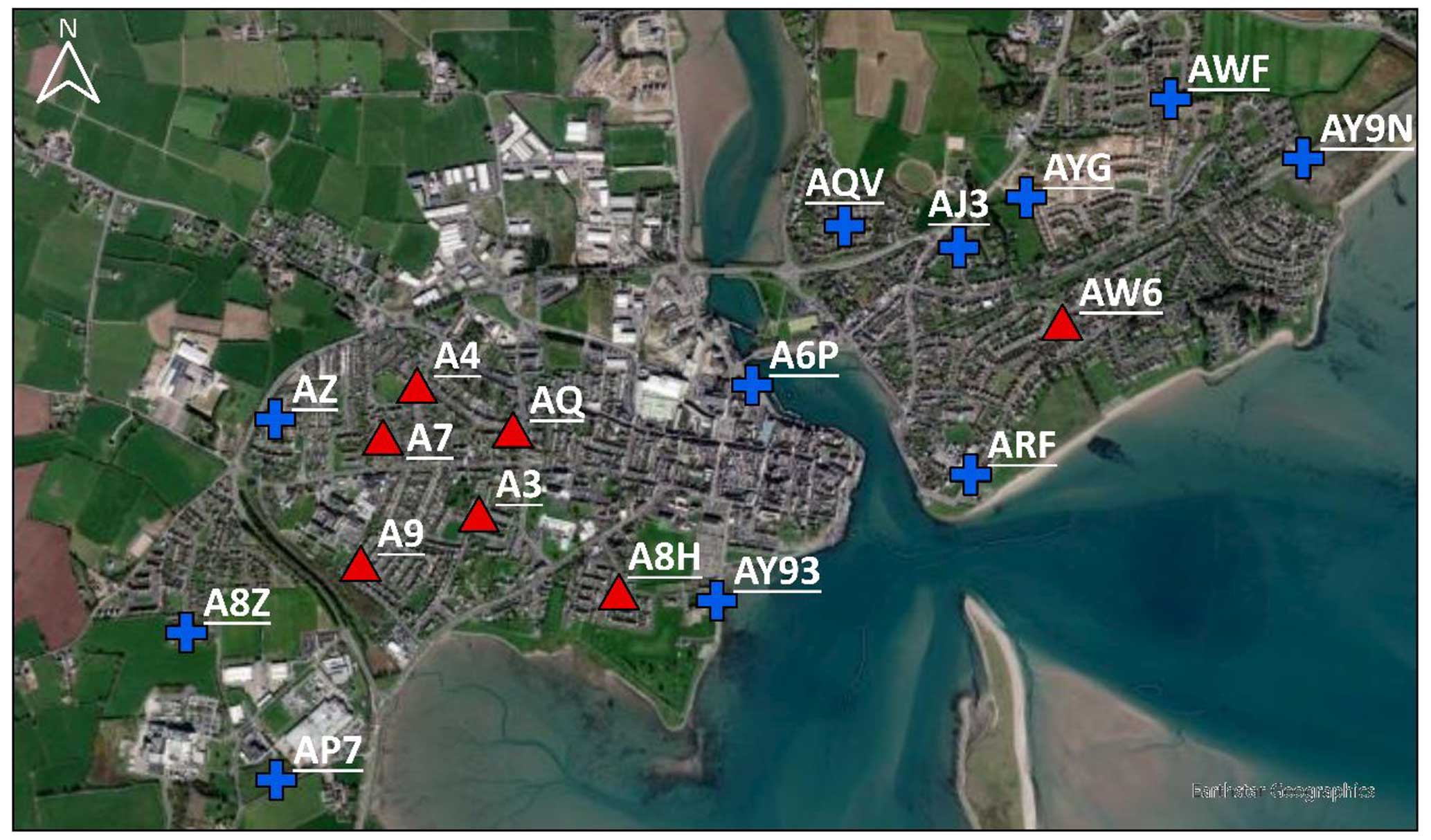
Figure 4 Dungarvan AQS locations with two cluster groups indicated. Cluster 1 devices (red triangle markers) are mainly located in central and residential areas, while Cluster 2 devices (blue cross markers) are mainly located on the edge of the town. (map obtained from Esri, DigitalGlobe, GeoEye, i-cubed, USDA FSA, USGS, AEX, Getmapping, Aerogrid, IGN, IGP, swisstopo, and the GIS User Community).

3.2 Cork PM_2.5 sensor network

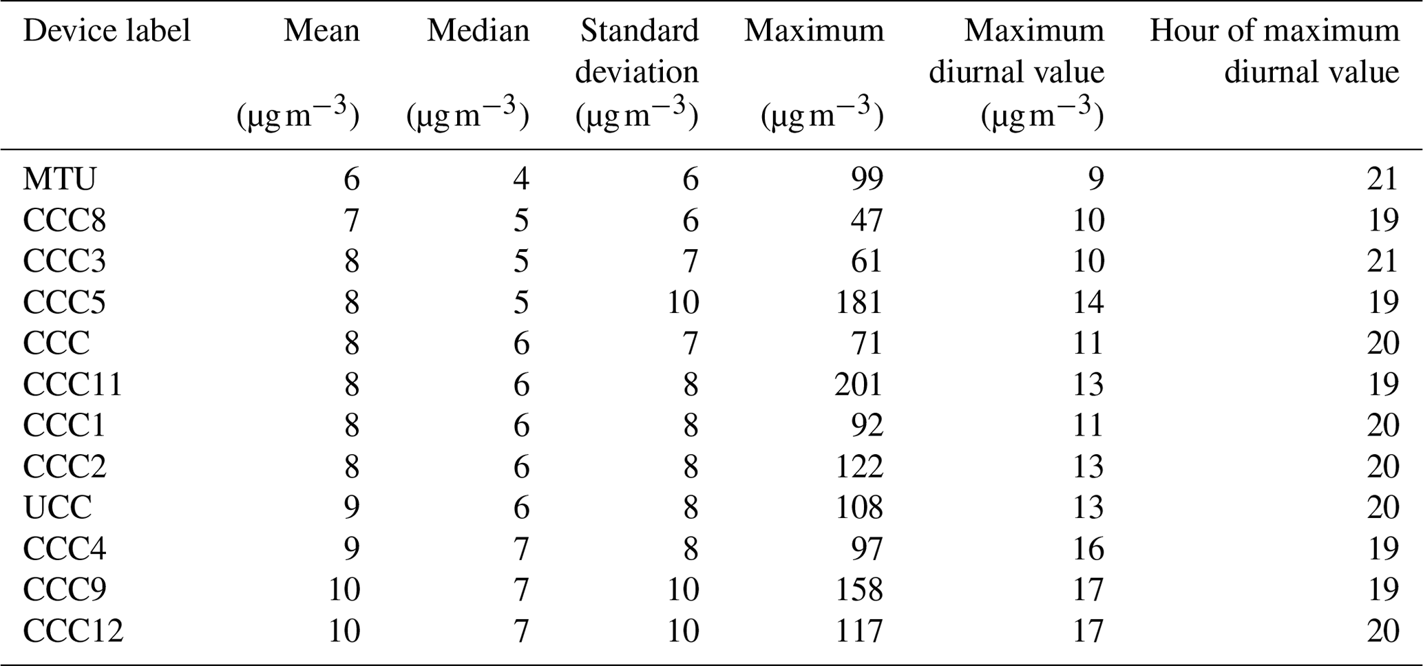
The same approach as above was used to analyse the data collected by the Cork AQS network. In this case, the corrected measurements are indicative of the actual PM_2.5 experienced in each location. The diurnal plots for each sensor in the Cork network are similar to those observed in Dungarvan, with a sizeable evening peak in PM_2.5 concentrations (19:00–21:00 LT) due to emissions from residential solid-fuel burning. Again, there is considerable variation in the peak concentration of PM_2.5 (Fig. 5). Device MTU showed the lowest diurnal average maximum of 9 µg m⁻³. This device is located on the western side of the city and has few upwind pollution sources contributing to air pollution at the location, as the prevailing wind direction is from the southwest. Devices CCC12 and CCC9 both showed the highest diurnal average maximum, 17 µg m⁻³. CCC12 is located northeast of the city and so likely experiences urban PM_2.5 sources upwind from it or has strong localised sources. Similarly, CCC9 is located to the east of the city in a residential area. Table 6 contains summary statistics for each of the sensors in the Cork network. Some devices had very high PM_2.5 maxima, e.g. 201 µg m⁻³ for CCC11, which were more than double the maxima of other devices, e.g. CCC8, which had the lowest overall maximum of 47 µg m⁻³. Device MTU had the lowest diurnal maximum value, indicating that this location was the least affected by local emissions from solid-fuel burning. However, it measured a significant overall PM_2.5 maximum of 99 µg m⁻³ and significant spikes in pollution were occasionally observed, likely due to meteorological conditions or specific localised effects. When looking at all of the parameters listed in Table 6, CCC11 stands out. This sensor has the highest maximum hourly average PM_2.5 concentration in the network, but the standard deviation (8 µg m⁻³) is in the middle of the range, indicating that the location had relatively stable PM_2.5 levels throughout the measurement period with less variation than other devices, but it was still susceptible to occasional spikes in PM_2.5.

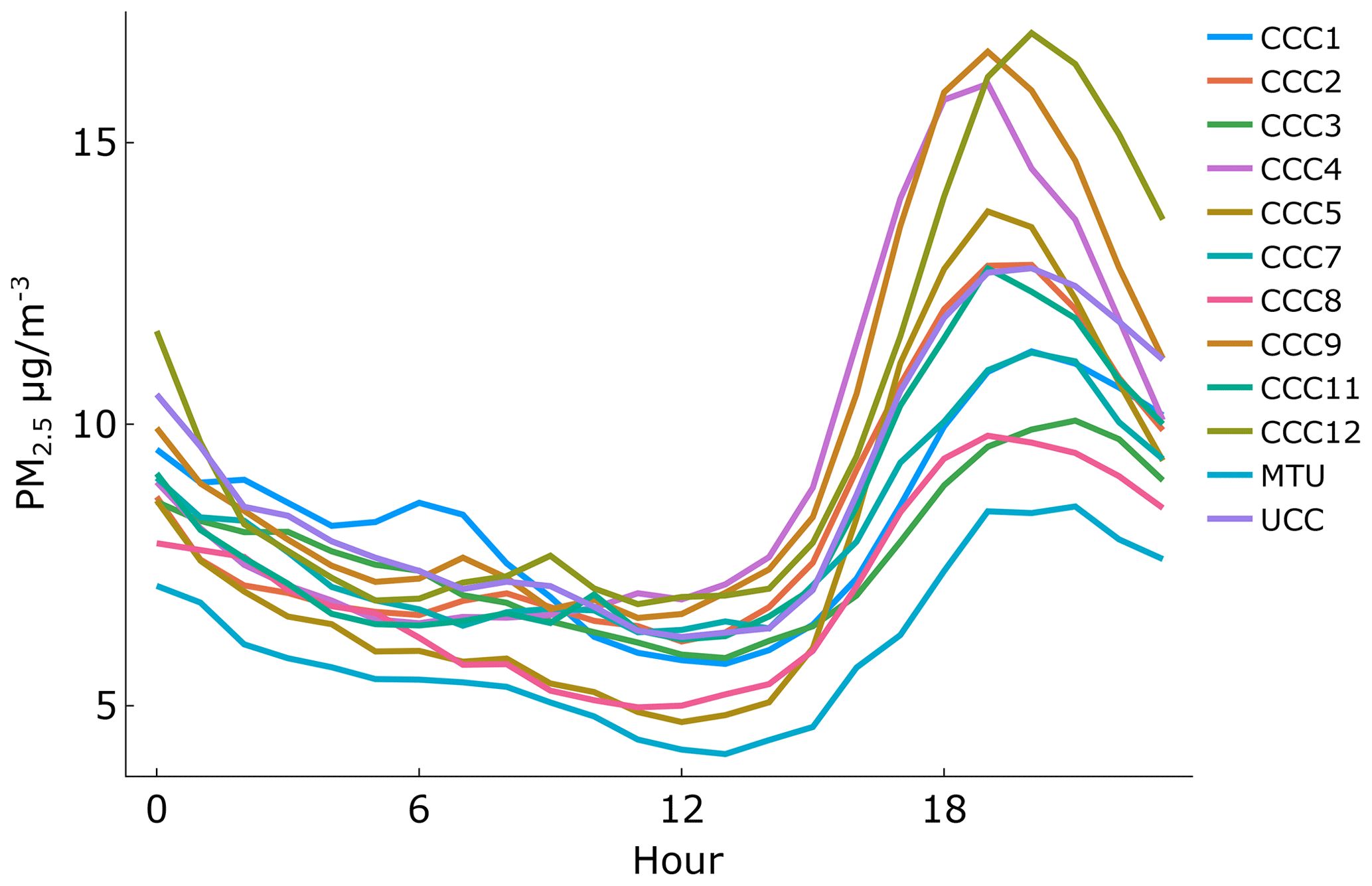
Figure 5 Diurnal PM_2.5 profiles for all AQSs in the Cork network (January to May and September to December 2021).

Table 6 Summary statistics of hourly averaged PM_2.5 obtained for all sensors in the Cork network (January to May and September to December 2021).

The meteorological data retrieved from Cork Airport, which is approximately 4–11 km from each device in the Cork sensor network, was investigated for the measurement period in 2021. While data obtained from the airport site indicates the meteorological conditions on a synoptic scale, the local weather experienced at individual locations within the city are additionally shaped by factors such as street canyon effects and local topography. Consequently, the wind direction measured at the airport site cannot be assumed to mirror that of all devices in the network. Wind speeds measured at the airport generally surpass those within the city as it is situated at a higher elevation than the city. However, the broader regional wind patterns are expected to exert a predominant influence on the overall meteorological conditions across the city, and therefore the relationship with meteorological conditions and local PM_2.5 levels can be investigated. The Cork Airport site recorded southerly winds 59 % of the time and southwesterly winds 39 % of the time (Fig. S8 in the Supplement).

3.2.1 Concentration similarity index

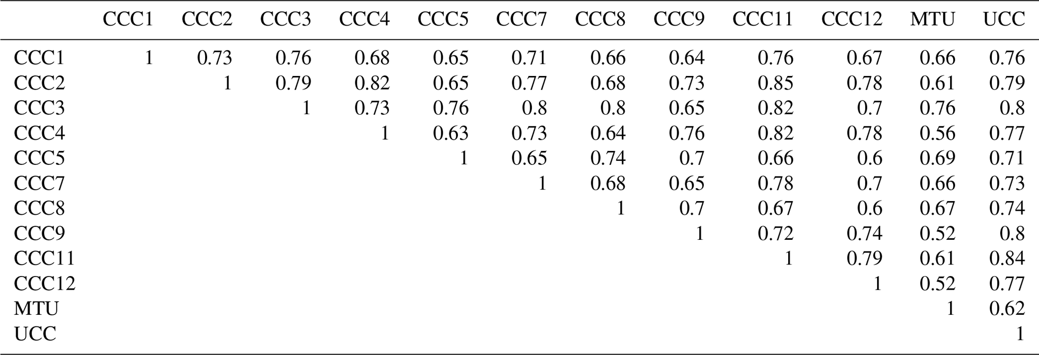
The matrix of CSI values obtained for the Cork sensor network is shown in Table 7. The values range from 0.52 (CCC12 vs. MTU and CCC9 vs. MTU) to 0.85 (CCC2 vs. CCC11) with a mean of 0.71. The high maximum CSI indicates a high degree of similarity between those locations in the network, and overall, Cork locations show a higher degree of similarity compared to those in Dungarvan.

Table 7 Concentration similarity indices for the hourly averaged PM_2.5 concentrations measured by PurpleAir devices in the Cork AQS network.

The isolated CSI results for the months of January and May 2021 were also assessed for the city of Cork. The average data coverage during both periods was 92 %. The mean CSI value in January (0.55) was considerably lower than that observed in May (0.82), Tables S6 and S7 in the Supplement. This result is similar to that found for the Dungarvan network, again indicating that the large difference in mean scores between the two months can be attributed to higher wintertime PM_2.5 variation due to residential solid-fuel burning (s_January=15 µg m⁻³, s_May=3 µg m⁻³).

3.2.2 Clustering

The two clustering algorithms were applied to investigate the CSI results of the Cork network. The silhouette scores for each number of assigned clusters (2 to 5) were low, with two clusters showing the highest mean score (Fig. S9 in the Supplement). Similarly, with the FCM analysis, two clusters showed the highest score with the Calinski–Harabasz indices (Fig. S10 in the Supplement).

The dendrogram produced from the hierarchical clustering and the membership weights for two clusters from FCM clustering are shown in Figs. 6 and 7, respectively. It is clear that devices MTU, CCC5, and CCC8 are all grouped together in one branch, Cluster 2, with the remainder of the devices in the other branch. The one assignment difference between the two clustering methods is CCC3, which has a higher membership weight towards Cluster 2 with the FCM method but does not branch with that cluster in the dendrogram. However, its membership weight is close to 0.5. CCC1 also shows a membership weight close to 0.5, however it is showing a higher weight towards Cluster 1, as per the hierarchical clustering results. Devices in Cluster 2, except for CCC3, all have the lowest mean CSI values.

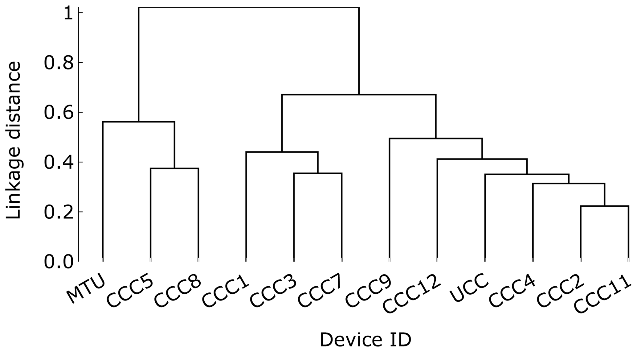
Figure 6 Dendrogram output from hierarchical clustering of the CSI data from the Cork sensor network.

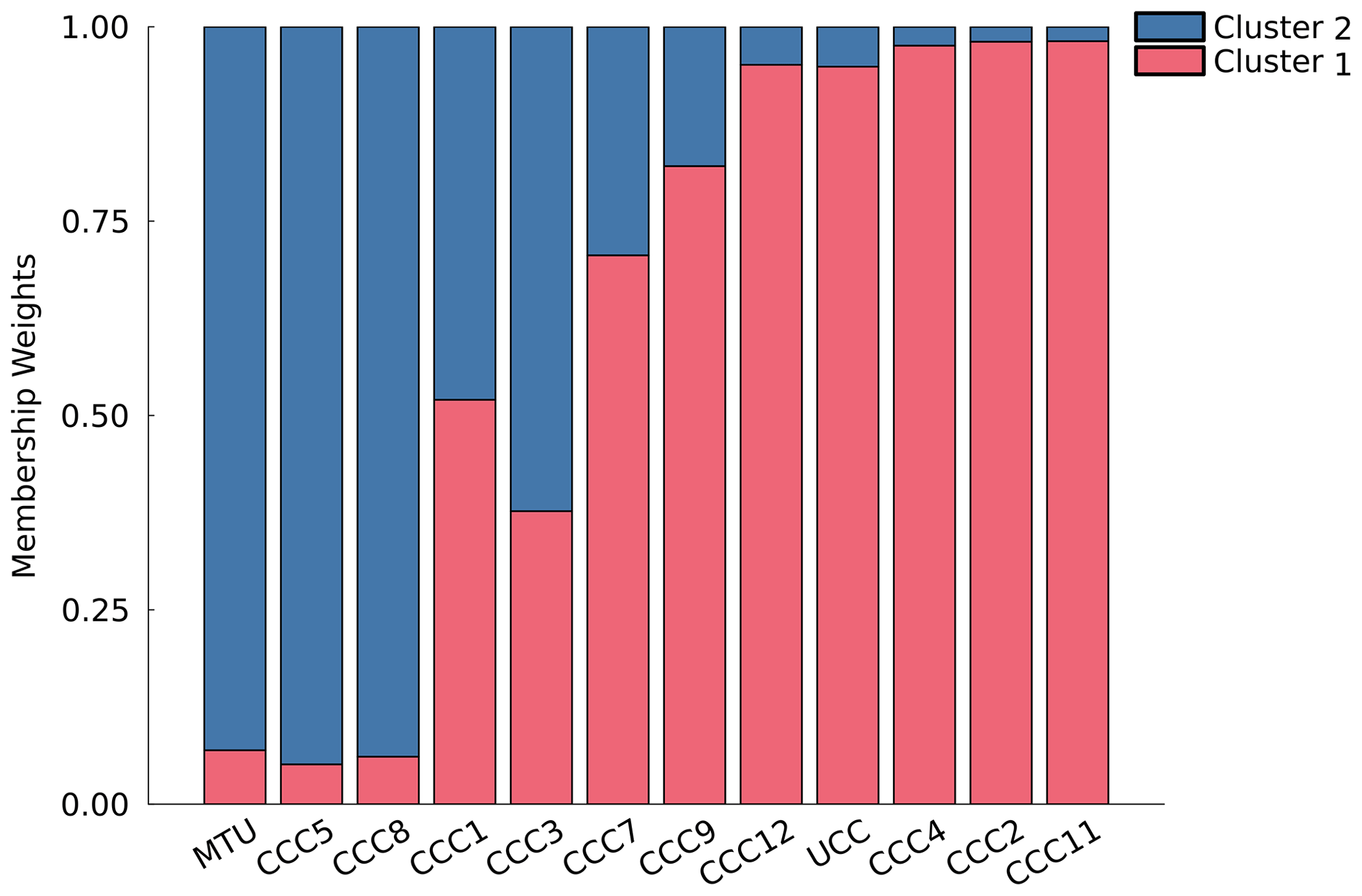
Figure 7 Membership weights from FCM clustering of the CSI data from the Cork sensor network.

Similar to the Dungarvan results, there appears to be a spatial component to the cluster groupings, with devices in Cluster 2 being mainly on the western side of the city, Fig. 8. However, the contrast in cluster PM_2.5 mean values is not as stark in the Cork clusters as in those in Dungarvan. Cluster 1 had a mean PM_2.5 of 9 µg m⁻³, while Cluster 2 had a mean PM_2.5 of 7 µg m⁻³. Interestingly, device CCC7, located in a commuter town on the western side of the city boundary, is grouped in Cluster 1 along with devices mainly in urban residential type sites instead of being grouped with other devices on the western edge of the city. This indicates that it has a more comparable CSI profile to the urban residential sites than the locations closer to it, further emphasising the importance of location type over physical proximity.

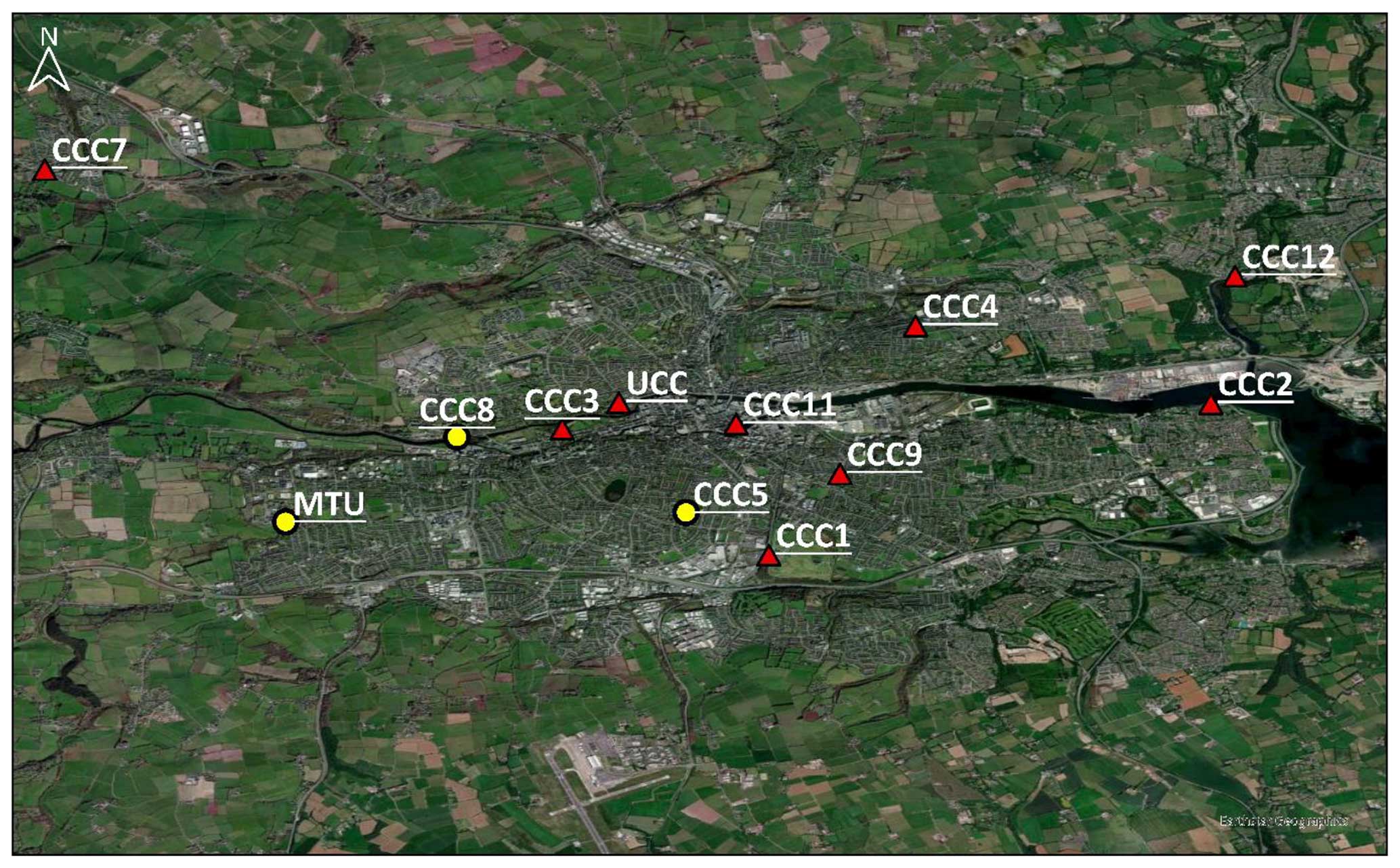
Figure 8 Cork AQS locations with two cluster groups indicated. Cluster 1 devices (red triangle markers) are located in the city centre and east/northeast, while Cluster 2 devices (yellow circle markers) are mainly located on the western side of the city. (map obtained from Esri, DigitalGlobe, GeoEye, i-cubed, USDA FSA, USGS, AEX, Getmapping, Aerogrid, IGN, IGP, swisstopo, and the GIS User Community).

3.3 Application of the CSI to assess representativeness of air quality monitoring locations

One key benefit of the CSI metric for AQS networks is that one sensor can be singled out and its overall degree of similarity to measurements from other locations can be determined. This analysis can be used to assess the spatial representativeness of a given location in the AQS network by quantitatively exploring how similar its PM_2.5 profile is to other locations. If a network sensor is co-located with a reference instrument, then the CSI values for that sensor can be used to provide a measure of the representativeness of the designated monitoring location and how well it informs the assessment of population exposure to air pollution.

In Dungarvan, the device A6P was co-located with a PM_2.5 instrument (Osiris, Turnkey) deployed as part of the national air quality monitoring network. The instrument is not a reference instrument but is certified to provide indicative measurements of PM_2.5 (National Ambient Air Quality Monitoring Network, 2023; Osiris, 2024). A6P had a mean CSI of 0.63, the fifth-highest of the mean CSI values across all devices. The similarity indices for A6P are included in Table 5 and represented spatially in Fig. 9. All CSI values are below the minimum threshold of 0.85 for two Clarity S-node devices in the Dungarvan network to be considered very similar. The most similar devices are found to the northeast of this location, AJ3 and AYG. Interestingly, the similarity of PM profiles does not decrease with increasing distance from A6P. Devices on the furthest western (AZ, A8Z, AP7) and eastern (AWF, AY9N) edges of the town are within 0.6 to 0.7, yet devices A4, A7, AQ, and A9 are all at or below 0.6 despite being physically closer to A6P. This suggests that the location type as opposed to physical proximity is more important when it comes to assessing the similarity of locations within Irish towns, as A4, A7, AQ, and A9 are all fully surrounded by residential areas, whereas the other devices mentioned are in more open areas.

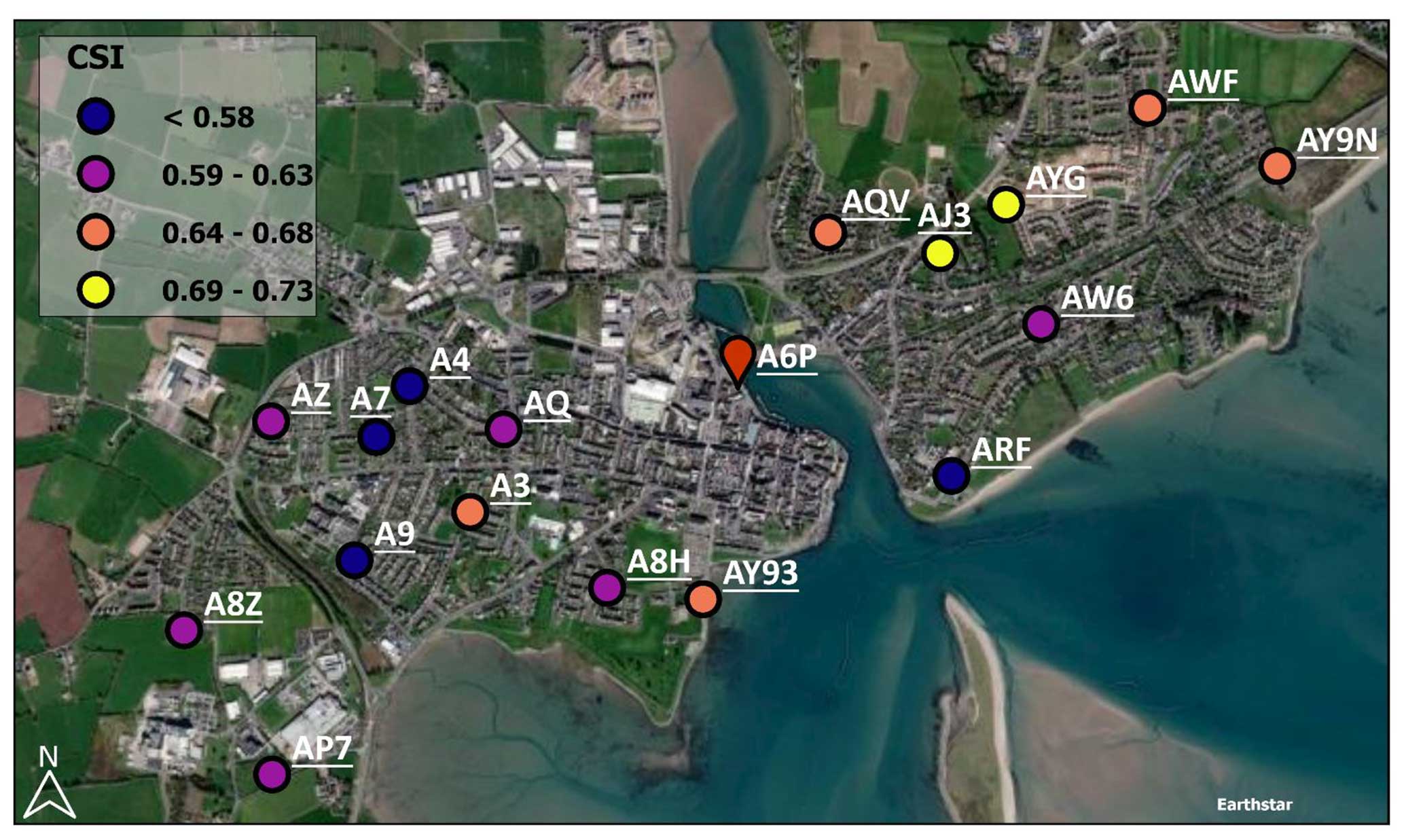
Figure 9 Dungarvan AQS locations with CSI results indicated in coloured circles (blue is the lowest CSI; yellow is the highest CSI) and the A6P location indicated by red pin marker. (map obtained from Esri, DigitalGlobe, GeoEye, i-cubed, USDA FSA, USGS, AEX, Getmapping, Aerogrid, IGN, IGP, swisstopo, and the GIS User Community).

One of the devices in the Cork sensor network, UCC, was co-located alongside a reference instrument (BAM-1020) at the national air quality monitoring location on the UCC campus. The CSI values for the device labelled UCC are shown in Fig. 10, showing how similar the measurements at this site are compared to the rest of the locations in the sensor network. The CSI scale on the map has been adjusted for these values. Similar to the Dungarvan case, there are devices that show high similarity (CCC4, CCC2, CCC12, CCC1) with UCC that are not located nearby.

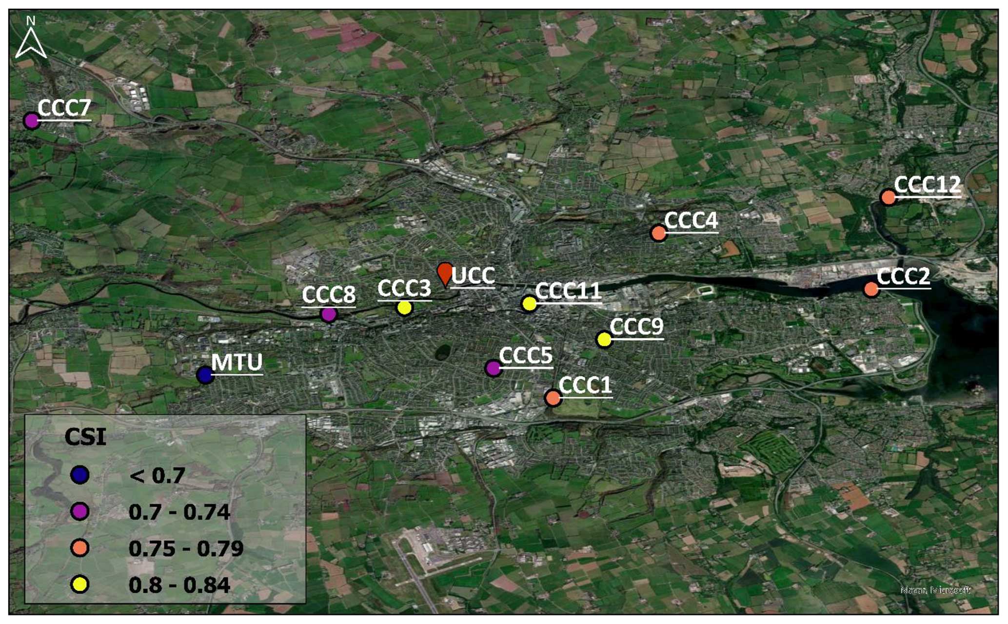
Figure 10 Cork AQS locations with UCC CSI results indicated in coloured circles (blue is the lowest CSI; yellow is the highest CSI) and the UCC location indicated by red pin marker. (map obtained from Esri, DigitalGlobe, GeoEye, i-cubed, USDA FSA, USGS, AEX, Getmapping, Aerogrid, IGN, IGP, swisstopo, and the GIS User Community).

4 Conclusion

A robust framework for comparing data series from individual air quality sensors in a network has been established, and a new metric, the concentration similarity index (CSI), has been developed, optimised, and tested on a co-location dataset. The CSI allows one to consider the monitoring network in terms of the similarity of the concentration–time profile of PM_2.5 at one location to profiles at the other locations in the same network. The harmonised dataset with minimal unexplained inter-sensor variation underpins the development of the CSI method, along with robust tests to ensure that the function represents an unbiased and fair depiction of the inter-sensor relationships after deployment in a monitoring network.

The CSI method has been used to analyse data generated by PM_2.5 sensor networks in two locations in Ireland: the coastal town of Dungarvan and the city of Cork. Clustering techniques are applied to the CSI matrix, and comparable similarity trends between locations drive the distinctions made with the clustering algorithm. The resulting groupings can provide several insights into the PM_2.5 profile at each location, including the likelihood of similarity in pollution sources, spatial patterns, and temporal trends. An interesting contrast in the CSI results from the two monitoring networks was obtained from the clustering analysis. In Dungarvan, the locations generated clusters that were reflected well when comparing the individual diurnal profiles and specifically the diurnal maximum values, indicating that this factor has a major influence when relating the concentration–time profiles at each location to one another in this network. However, for the Cork network results, this was not as apparent. The clusters were not aligned based on diurnal peaks, but rather the differentiating factor was more nuanced. Both clusters contained locations with a mix of higher and lower diurnal maxima and overall maxima. However, both network groupings reflect the fact that devices may report dissimilar CSI results to other devices located nearby and that considering location specifications or types, such as residential areas, is more important than physical proximity when it comes to understanding and quantifying the similarities between locations.

The CSI function was also applied to two separate months in the network datasets, with January chosen to represent a period of higher PM_2.5 levels due to solid-fuel burning emissions and May chosen to represent a period with lower PM_2.5 concentrations due to reduced solid-fuel burning. In both locations, the mean CSI for the network comparisons was higher in May than in January, indicating that higher PM_2.5 levels are a major driver of lower similarity indices between sensor locations. Combining this with the findings of our previous study, we provide further evidence that high levels of localised PM_2.5 cause distinct disparities in exposure to poor air quality in different locations. Furthermore, to properly assess the burden of PM_2.5 experienced by a population and to accurately compare the measurements at two locations, the wintertime PM data must be included in the assessment.

The similarity of PM_2.5 measured at designated sites in the national air quality monitoring network compared to the rest of the locations in the sensor networks was analysed to give an estimation of the representativeness of the air pollution measured at the designated monitoring site. The national monitoring site location in Dungarvan was shown to be moderately representative of the other AQS network locations in the town, with CSI values ranging from 0.53 to 0.72. The CSI values for the Cork comparison ranged from 0.62 to 0.84, also showing a fair representation of the air pollution experienced in the rest of the network. The CSI function was also tested via synthetic datasets, which showed that a positive offset of just 5 µg m⁻³ resulted in almost halving the CSI, which was a lower CSI than most of the sensor comparisons in both network locations. So, while a CSI of 0.85 was used as a limit for two sensor measurement sets being very similar, CSI values between 0.6 and 0.7 are still moderately similar. In general, the CSI values in the city of Cork for the reference site comparison were higher (mean=0.75) than that of Dungarvan (mean=0.63), indicating less similarity between the reference site and devices in the Dungarvan network compared to those in the city of Cork.

While the function was developed and tested on multiple sensor pairs and further validated with additional co-located pairs, validation with co-located PM_2.5 measurements of the PM_lim, C_{lim, upper}, and C_{lim, lower} parameters for specific applications is recommended to ensure that the index represents the dataset accurately. Co-location assessments are also recommended to ensure minimal inter-sensor variation. Nonetheless, the differentiation between higher and lower PM values in the concentration similarity assessment is a strategic choice that acknowledges the complexity of PM_2.5 data, the varying significance of concentration levels, and the limitations of sensors. It allows for a more accurate representation of similarities, while considering real world implications and measurement uncertainties, and minimises the potential biases that could arise from an indiscriminate approach, thus ensuring an impartial and unbiased evaluation.

The analysis and application of the CSI function displays the potential for AQS networks to be used in conjunction with a regulatory monitoring system. This study has shown the potential for sensor networks to assess the need for more regulatory monitoring in an area and to identify locations that are being poorly represented by the current system. Furthermore, the CSI method can be used to optimise a sensor network by carrying out short-term sensor deployments and identifying areas of similarity or dissimilarity and thus assessing where the best locations for sensors are, based on the similarity in exposure to air pollution.