Multi-instrumental analysis of ozone vertical profiles and total columns in South America: comparison between subtropical and equatorial latitudes

The behavior of ozone gas (O₃) in the atmosphere varies according to the region of the globe. Its formation occurs mainly in the tropical stratosphere through the photodissociation of molecular oxygen with the aid of the incidence of ultraviolet solar radiation. Still, the highest concentrations of O₃ content are found in high-latitude regions (poles) due to the Brewer–Dobson circulation, a large-scale circulation that takes place from the tropics to the pole in the winter hemisphere. This work presents a multi-instrumental analysis at two Brazilian sites, a subtropical one (Santa Maria – 29.72° S, 53.41° W) and an equatorial one (Natal – 5.4° S, 35.4° W), to investigate ozone distributions in terms of vertical profiles (2002–2020) and total abundance in terms of total columns of ozone (1979–2020). The study is based on the use of ground-based and satellite observations. Ozone profiles over Natal, from the ground up to the mesosphere, are obtained by radiosonde experiments (0–30 km) in the framework of the SHADOZ program and by satellite measurements from the SABER instrument (15–60 km). This enabled the construction of a continuous time series for ozone, including monthly values and climatological trends. There is a good agreement between the two measurements in the common observation layer, mainly for altitudes above 20 km. Below 20 km, SABER ozone profiles showed high variability and overestimated ozone mixing ratios by over 50 %. Dynamic and photochemical effects can interfere with O₃ formation and distribution along higher latitudes through the Brewer–Dobson circulation. The measurements of the total ozone columns used are in good agreement with each other (TOMS/OMI × Dobson for Natal and TOMS/OMI × Brewer for Santa Maria) in time and space, in line with previous studies for these latitudes. Wavelet analysis was used over 42 years. The investigation revealed a significant annual cycle in both data series for both sites. The study highlighted that the quasi-biennial oscillation (QBO) plays a significant role in the variability of stratospheric ozone at the two study sites – Natal and Santa Maria. The QBO's contribution was found to be stronger at the Equator (Natal) than at the subtropics (Santa Maria). Additionally, the study showed that the 11-year solar cycle also has a significant impact on ozone variability at both locations. Given the study latitudes, the ozone variations observed at the two sites showed different patterns and amounts. Only a limited number of studies have been conducted on stratospheric ozone in South America, particularly in the region between the Equator and the subtropics. The primary aim of this work is to investigate the behavior of stratospheric ozone at various altitudes and latitudes using ground-based and satellite measurements in terms of vertical profiles and total columns of ozone.

1 Introduction

About 90 % of the atmospheric ozone content is found in the stratosphere between 15 and 35 km altitude (London, 1985; WMO, 1998). In this altitude range, the formation of a protective barrier against UV radiation harmful to human health and to the biosphere is observed in the well-known ozone layer (Kirchhoff et al., 1991). A combination of dynamic and photochemical processes determines the abundance of ozone concentration in the stratospheric layer. Thus, in the upper stratosphere (35–50 km), the ozone abundance is determined by the photochemical production and destruction processes of this gas (Chapman, 1930), while in the lower stratosphere (15–30 km), the abundance of O₃ is mainly controlled by dynamical processes (Dobson et al., 1930; Brewer, 1949; Bencherif et al., 2007, 2011).

Several instruments have been used to improve the analysis and understanding of atmospheric ozone. Vertical analysis of ozone content is important because it contributes to better understanding of O₃ distributions in the troposphere and in the stratosphere. Ozone in the atmosphere is measured by various experiments from the ground or onboard satellites. The Sounding of the Atmosphere using Broadband Emission Radiometry (SABER) instrument aboard the TIMED (Thermosphere Ionosphere Mesosphere Energetics Dynamics) satellite (TIMED/SABER; Russell et al., 1999) has been providing continuous ozone profiles since 2002. They were used in this study to investigate ozone distributions and variations with height and time over tropical and subtropical latitudes. SABER data were used in several studies on ozone and temperature variability (Dutta et al., 2022). Remsberg et al. (2003) reported on the behavior of the SABER temperature profiles for February 2002 between 52° S and 83° N. They showed that these data are useful for analyzing the dynamics and transport of chemical tracers in the middle atmosphere. Nath and Sridharan (2014) identified the main variabilities and trends in O₃ content and temperature behavior using SABER data between 20 and 100 km altitude in the 10–15° N region between 2002–2012. Their results showed an intense biannual oscillation during March to May and August to September (between 25 and 30 km altitude). Joshi et al. (2020) analyzed the seasonal and annual cycle variability of O₃ over 14 years of SABER data (2002–2015) in mid-latitude regions of both hemispheres. The results by Joshi et al. (2020) showed an accumulation of O₃ starting in late winter and peaking in early spring in both hemispheres, underlining the dynamical effects induced by the polar vortex and pre-formation of the Antarctic ozone hole (AOH). In addition, they showed that the annual cycle occurred in the middle atmosphere of both hemispheres (between the stratosphere and the lower mesosphere), while the semi-annual cycle peaked between 40–60 and 80–100 km altitude.

Ozonesonde measurements proved to be effective in tropospheric and stratospheric ozone analysis (Thompson et al., 2003a, b; Diab et al., 2004, Bencherif et al., 2020, 2024), and the SHADOZ network presents a wide area of ozonesonde measurements mainly deployed at tropical latitudes. In this way, using satellite instruments helps to investigate the vertical distribution of O₃ in different latitudes of the globe, other than tropical regions, and to characterize its vertical distribution. Sivakumar et al. (2007) reported on O₃ variability and climatology in the stratospheric layer over Reunion Island (21.06° S, 55.31° E), using satellite (HALOE, SAGE-II, TOMS) observations in combination with ground-based measurements, i.e., radiosondes, and a UV–visible spectrometer (SAOZ, Système d'Analyse par Observations Zénithales). Due to the limited number of radiosondes carried out at SM, a comparison between radiosondes and SABER was only made for the equatorial site Natal. Natal is one of the oldest ozone stations in South America, with a record of ozone profiles dating back to 1979, although there are large gaps in the data. The most continuous ozone profile experiment in Natal is a weekly based one, which started in 1998 in the SHADOZ framework. Thus, in this work, only comparisons between measurements of the vertical profiles of the atmosphere recorded at Natal were used. Latitudinal differences can modulate the content and variability of O₃ in different layers of the atmosphere, mainly due to the characteristics of each region in terms of seasonal and dynamic forcings (Reboita et al., 2010). To investigate these latitudinal differences in ozone distributions, ozone measurements at two Brazilian stations were used, i.e., Santa Maria in the subtropical region and Natal in the equatorial region. Two kinds of ozone data are combined as derived from ground and satellite observations: vertical profile and total column ozone (TCO) data. Analysis of the TCO times series for both sites (both latitudinal regions) is based on over 42 years of quasi-continuous measurements (1979–2020). The Santa Maria (SM; 29.72° S, 53.41° W) station is in the suburb of the city of Santa Maria in the central region of the state of Rio Grande do Sul. This region in the south of Brazil is subject to dynamical and indirect effects of the polar vortex disturbances and of the Antarctic ozone hole during its active periods. The Natal (NT; 5.42° S, 35.40° W) station is an equatorial one. The Natal site is one of the oldest ozone stations in Brazil and Latin America. Globally, the two locations (SM and NT) are the most important stations in Brazil, with ground-based total ozone measurements which began monitoring in 1992 for SM and in 1994 for NT.

Additional measurements and continuous monitoring of ozone, especially through radiosonde observations, are necessary in mid-latitudes and subtropical latitudes of the Southern Hemisphere, such as Santa Maria. In fact, some balloon sondes were launched in SM but not enough for a long-term comparison of O₃ content. Therefore, radiosonde data recorded at Natal were used to validate satellite ozone observations as obtained over Natal by the TIMED/SABER overpasses from 2002 to 2020. In this work, after inter-comparing ozone profiles and validating TIMED/SABER satellite data for the Natal site, the obtained ozone time series were analyzed and compared for the two study regions (equatorial – NT and subtropical – SM) to identify the main characteristics in terms of ozone behavior during the study period. The combination of TCO time series obtained from satellite measurements (TOMS and OMI) and from ground-based Brewers and Dobson spectrometers allowed us to extend TCO time series over a large period of 42 years for both stations (Santa Maria and Natal). The TCO series obtained are used for the analysis of interannual and intra-annual variability, allowing for a comparison between the two study regions.

2 Database and methodology

2.1 Regions of study and data

This work consists of a multi-instrumental analysis of the vertical profile of stratospheric ozone and the TCO to investigate ozone variability at different latitudes in Brazil. The selected Brazilian sites are Santa Maria (SM), in the subtropics, and Natal (NT), near to the Equator. SM is a region under strong dynamics, leading to the variability of O₃ throughout the year. It is characterized by a baroclinic atmosphere, under influences of the passage of frontal systems and cold fronts, as well as the proximity of the jet stream (Shapiro and Keyser, 2015). The associated winds are crucial in the vertical distribution of O₃, being considered the main tropospheric pattern directly linked to the transport of O₃ from the stratosphere to the troposphere. The position and speed of the jet streams (subtropical or polar), because of change or discontinuity in the meridional temperature gradient, can determine the ozone variation in the atmosphere (Reboita et al., 2010; Bukin et al., 2011). These dynamical contexts in subtropical latitudes have significant relevance in studies with O₃ because they have an indirect relationship with the Antarctic ozone hole (AOH), which modifies the O₃ content in the region, mainly during the austral spring through the ejection of air masses with low O₃ content from the polar region, where the Antarctic ozone hole is located, to the subtropics, as was observed and reported for the SM location (Kirchhoff et al., 1996; Vaz Peres et al., 2017; Bittencourt et al., 2018, 2019).

The equatorial region of Brazil (NT) presents a barotropic atmosphere with less variation in the temperature gradient. According to Reboita et al. (2010), the Brazilian northeast region near to the Equator experiences different meteorological systems throughout the year, thus impacting the accumulated precipitation. In this region, the primary driver of weather systems is thermodynamics, unlike in higher latitudes, where dynamic forcing is more common. During the wet season (which runs from November to March), the area experiences daily bouts of rainfall caused by the Intertropical Convergence Zone (ITCZ) shifting towards the summer hemisphere. The circulation of the breeze helps to transport humidity throughout the region, while the South Atlantic high pressure also contributes by causing radiative heating and increasing humidity, which in turn leads to convection. Some studies showed that in the future, there is a possible trend of acceleration of the Brewer–Dobson circulation (BDC) in the lower stratosphere region, mainly caused by the increase in greenhouse gases in the atmosphere (Weber et al., 2011; WMO, 2022). In addition, NT has one of the oldest SHADOZ stations, with data available since 1998 (Thompson et al., 2003a, 2017; Witte et al., 2017). Ozone profiles recorded by radiosondes at this station are used to validate SABER satellite observations. Figure 1 depicts the map of South America, highlighting the two Brazilian study sites, SM and NT.

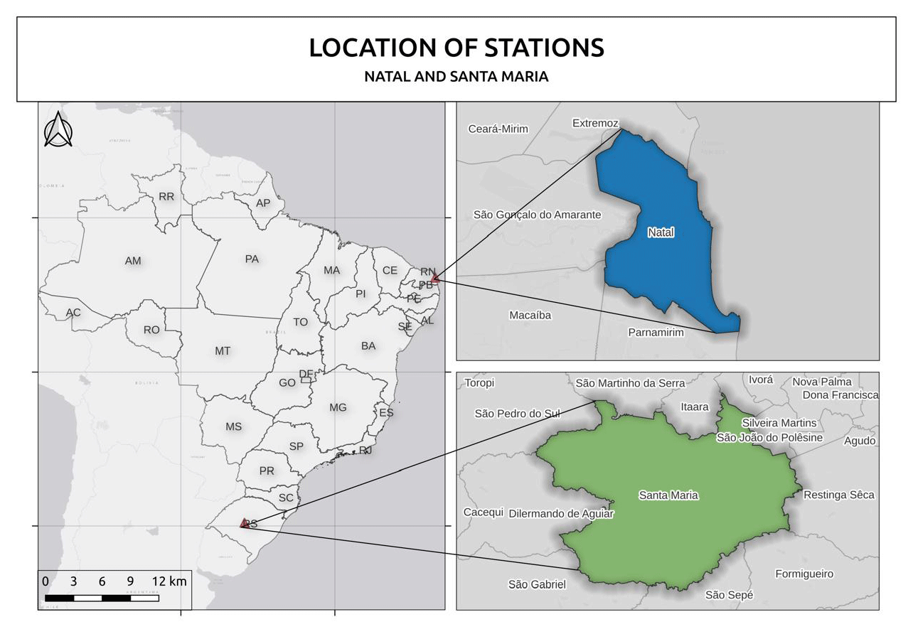
Figure 1 Map of South America showing the two stations used in this work, Natal (RN) at equatorial latitude and Santa Maria, a subtropical region of Brazil.

2.1.1 Database: SHADOZ observations

The SHADOZ program has been operating since 1998. It brings together 14 stations equipped to measure ozone profiles from the ground up to the stratosphere (∼ 30 km) by a balloon-sonde experiment in the tropics and sub-tropics (Thompson et al., 2003a). The ozone concentration is measured in situ by an electrochemical cell (ECC), simultaneously with pressure, temperature, and humidity measurements during the balloon's ascent. In South America, the SHADOZ network has a station in NT, which has been in operation since 1998. A period of 19 years of data was analyzed using the new version available at https://tropo.gsfc.nasa.gov/shadoz/Natal.html, (last access: 12 October 2023), which offers many variables: ozone, temperature, pressure, relative humidity, wind direction, and speed (Thompson et al., 2021). From this, ∼ 580 daily profiles were obtained at Natal from 2002 to 2020. Indeed, ozone and temperature profiles obtained from balloon sondes were vertically interpolated from the surface up to ∼ 30 km altitude, with a resolution of 50 m, which corresponds to 604 altitude bins.

2.1.2 Database: vertical ozone data

TIMED/SABER observations

In this work, vertical ozone profiles were used to investigate ozone variability over the study sites, SM and NT. This was based on satellite-based measurements from the SABER instrument on board the TIMED (Thermosphere-Ionosphere-Mesosphere Energetics and Dynamics) satellite (Russell et al., 1999; Dawkins et al., 2018), which has been operating since 2002. The SABER instrument observes the Earth in narrow spectral ranges, with high accuracy of carbon dioxide (15 µm), ozone (9.6 µm), and nitric oxide (5.3 µm) emissions (Mlynczak et al., 1993, 2007). The main objective of the SABER experiment is to better understand fundamental atmospheric processes in the middle atmosphere and the thermosphere (Russell et al., 1999; Joshi et al., 2020). SABER is one of four experiments on NASA's TIMED mission, launched in May 2000 by a Delta II rocket into a circular orbit 74.1° ± 0.1° inclined, with an area of 625 ± 25 km. It provides vertical profiles of ozone and temperature in the 15–110 km altitude range. Ozone profiles measured by SABER are known to have good accuracy at altitudes above 20 km, and this accuracy tends to drop off at lower altitudes in the upper troposphere–lower stratosphere (UTLS; Wing et al., 2020). In fact, Wing et al. (2020) compared SABER ozone profiles during the Lidar Validation NDACC Experiment at the Observatoire de Haute-Provence and found good agreement between SABER and other ozone measurements from lidar and SHADOZ data between 20 and 40 km, with less than ∼ 5 % differences. They also showed that below 20 km, SABER measurements significantly overestimate ozone compared to the lidar or SHADOZ. Given the availability of ozone profiles measured by radiosondes at the Natal site, this study aims at the first stage to compare the SABER and SHADOZ ozone profiles obtained in the 15–30 km altitude range over NT during the common period, between 2002 and 2020. One of the aims of this study is to provide a detailed comparison of the vertical behavior of ozone in the subtropical latitudes of Brazil, particularly at SM. To do this, we used data from the SABER satellite, since unlike Natal this region does not currently have a station for continuous measurement of vertical ozone profiles. For this work, the SABER OMR (ozone mixing ratio) profiles were selected at ±2° in latitude and longitude from the coordinates of the NT and SM study sites. During the 19 years of data, approximately 6715 daily OMR vertical profiles were identified where the satellite mapped the SM and 3681 daily vertical profiles for NT from 2002–2020. This means that the SABER OMR profiles over SM are expected to have greater statistical power for variability and trend analysis than those for NT. The profiles were interpolated with a vertical resolution of 0.1 km, providing 954 altitude levels in the 15 to 110 km height range. The SABER satellite provides data on altitude (in km), latitude and longitude, temperature (in kelvin), and OMR (in ppmv). Complementary analysis includes monthly mean and climatology of the OMR profile over the two study regions.

2.1.3 Database: total column ozone data

The TCO measurements were also used in this work, as available ozone data spanning 42 years at the two latitudes were studied, along with data from satellites and ground-based instruments. The period for TCO analysis was between 1979 and 2020, using mainly ground-based instruments (Brewer spectrophotometer and Dobson spectrophotometer) and satellite instruments (TOMS, OMI). For SM, the ground-based instrument used is the Brewer spectrophotometer, which performs daily measurements of ultraviolet radiation, the TCO, and sulfur dioxide column (SO₂). The beginning of TCO monitoring in SM started with the Brewer spectrophotometer model MkIV no. 081 from 1992 to 1999, while the model MkII no. 056 operated from 2000 to 2002, and the model MkIII no. 167 operated from 2002 to 2017. For NT, the ground-based instrument used was the Dobson spectrophotometer no. 093. The Dobson instrument is a dual-beam monochromator that measures the TCO through absorbed radiation at two wavelengths (305.5 and 325.4 nm) by direct sun (DS) observations, measured since 1978 in NT.

Satellite TCO time series were obtained from two main instruments: from the Total Ozone Mapping Spectrometer (TOMS) and the Ozone Monitoring Instrument (OMI) experiments. The TOMS instrument began its activities in 1978, with the launch of the Nimbus-7 satellite, and it remained operational until 1994. In 1991, the Meteor-3 satellite was launched and provided TOMS measurements until December 1994, when it was replaced by the Earth Probe satellite in August 1996, and it remained in operation until December 2006. The TOMS instrument ended its activities on December 2005, while OMI has been operating since July 2004 aboard the AURA satellite. OMI is derived from the TOMS and from the Global Ozone Monitoring Experiment (GOME) on board the ERS-2 satellite.

In comparison with TOMS and GOME, OMI can measure more atmospheric constituents at better horizontal resolution (13 km × 25 km for OMI vs. 40 km × 320 km for GOME). This study analyzed the monthly time series of the TCO from both NT and SM stations. The measurements were mainly based on ground-based instruments, i.e., Dobson and Brewer spectrometers, respectively. However, some data were missing, and to fill those gaps, satellite measurements were used like the method followed by Vaz Peres et al. (2017) and Sousa et al. (2020). The TCO time series for NT and SM were created by filling in the gaps with TOMS and OMI data, successively. This covered the study period from 1979 to 2020. The resulting TCO time series were then analyzed on a statistical and analytical basis using the wavelet transform to study ozone variability.

2.2 Statistics, comparisons, and variabilities

The investigation of the ozone content at the two selected stations over these 42 years of data, consisting of onboard satellite instruments (TOMS, OMI) and ground-based instruments (Brewer, Dobson, SHADOZ), has distinct particularities that are of paramount importance in monitoring ozone content in tropical and subtropical latitudes. Statistical analyses were performed on the obtained TCO time series. Comparisons were made between different types of instruments (TOMS/OMI × Brewer/Dobson). Through the monthly TCO time series over 42 years, the following calculations were performed.

$$\begin{array}{}\text{(1)}& \begin{array}{rl}& {\mathrm{Pearson}}^{\prime }\mathrm{s}\mathrm{correlation}\mathrm{coefficient}\left(R\right):\\ & R=\\ & {\displaystyle \frac{{\sum }_m{\sum }_n(\mathrm{satellite}-\stackrel{\mathrm{‾}}{\mathrm{satellite}})\left(\mathrm{Brewer}-\stackrel{\mathrm{‾}}{\mathrm{Brewer}}\right)}{\sqrt{\left({\sum }_m{\sum }_n\right(\mathrm{satellite}-\stackrel{\mathrm{‾}}{\mathrm{satellite}}{)}^{\mathrm{2}}\left({\sum }_m{\sum }_n\right(\mathrm{Brewer}-{\stackrel{\mathrm{‾}}{\mathrm{Brewer}}}^{\mathrm{2}}\left)\right)}}}.\end{array}\end{array}$$

The R² shown in the results is the value of the squared correlation coefficient. The root mean square error (RMSE), often used to estimate the difference between the values predicted by a model (which, in this case, is a satellite) and the observed values (Brewer spectrophotometer), aggregates the predictive strength of the variable in a single measurement.

$$\begin{array}{}\text{(2)}& \begin{array}{rl}& \mathrm{Root}\mathrm{mean}\mathrm{square}\mathrm{error}\left(\mathrm{RMSE}\right):\\ & \mathrm{RMSE}=\sqrt{{\sum }_{i=\mathrm{1}}^n{{\displaystyle \frac{\left(\mathrm{satellite}i-\mathrm{Brewer}i\right)}{n}}}^{\mathrm{2}}}.\end{array}\end{array}$$

The mean bias error (MBE) represents a systematic error in which positive values of MBE represent an overestimation of the data and negative values an underestimation of the observed data relative to the satellite data.

$$\begin{array}{}\text{(3)}& \begin{array}{rl}& \mathrm{Mean}\mathrm{bias}\mathrm{error}\left(\mathrm{MBE}\right):\\ & \mathrm{MBE}={\displaystyle \frac{\mathrm{100}}{n}}{\sum }_{i=\mathrm{1}}^n{\displaystyle \frac{\left(\mathrm{satellite}i-\mathrm{Brewer}i\right)}{\mathrm{Brewer}i}}.\end{array}\end{array}$$

Statistical calculations enable a quantitative analysis of each instrument and each region studied. Regarding the vertical distribution of ozone, simultaneous OMR profiles were analyzed. On this basis, the coincident OMR monthly profiles from SABER and SHADOZ were used and compared for NT and SM. The percentage relative differences (RDs) were calculated as given by Eq. (4):

$$\begin{array}{}\text{(4)}& \mathrm{RD}\left(\mathit{\%}\right)=\mathrm{100}\cdot {\displaystyle \frac{(\mathrm{SABER}-\mathrm{SHADOZ})}{\left(\mathrm{SHADOZ}\right)}}.\end{array}$$

2.2.1 Ozone variabilities

This section presents the results on ozone variability based on time series constructed over a 42-year period. The wavelet transform method was used by many authors to identify the dominant forcings governing this variability (Torrence and Compo, 1998; Rigozo et al., 2012). Monthly TCO anomalies were used in the wavelet transform method to reveal the main modes of ozone variability (Hadjinicolaou et al., 2005). In this work, we used the Morlet transformed wavelet. It comprises a Gaussian function modulating a plane wave, represented by

$$\begin{array}{}\text{(5)}& {\mathrm{\Psi }}_{\mathrm{0}}\left(\mathit{\eta }\right)=\mathit{\pi }{\displaystyle \frac{\mathrm{1}}{\mathrm{4}}}{e}^{i{\mathit{\omega }}_{\mathrm{0}}\mathit{\eta }}{e}^{\frac{-{\mathit{\eta }}^{\mathrm{2}}}{\mathrm{2}}},\end{array}$$

where ω₀ is the non-dimensional frequency, and η is the non-dimensional time parameter. Considering the discrete time series (X_n), with a fixed time spacing (Δt) and n=0, $\mathrm{\dots },N-\mathrm{1}$, the continuous wavelet transform is in Eq. (6):

$$\begin{array}{}\text{(6)}& W_n\left(s\right)={\sum }_{n^{\prime }=\mathrm{0}}^{N-\mathrm{1}}{X}_n{\mathrm{\Psi }}^{*}\left[{\displaystyle \frac{(n{}^{\prime }-n)\mathrm{\Delta }\mathrm{t}}{s}}\right],\end{array}$$

where (^*) is the complex conjugate in the period (wavelet scale). The global wavelet spectrum in Eq. (7) allows for calculating the unbiased estimate of the real power spectrum of the time series by calculating the average wavelet spectrum over a period.

$$\begin{array}{}\text{(7)}& W^{\mathrm{2}}\left(s\right)={\displaystyle \frac{\mathrm{1}}{N}}{\sum }_{n=\mathrm{0}}^{N-\mathrm{1}}\left|W_n\left(s\right)\right|\end{array}$$

The wavelet transform analysis is a highly effective mathematical and numerical tool that provides the power spectrum of a series analyzed as a function of time. The edge effects are displayed as a U-shaped curve called the cone of influence. Within this cone, the confidence level is set at 95 %, marking the boundary for the most significant results from the analyzed data series.

To investigate the percentage contributions of the main modes of ozone variability, the multilinear regression model Trend Run was used. This model was adapted by LACy at the University of Reunion and has been successfully applied to various time series of atmospheric parameters, particularly temperature and ozone series (Bencherif et al., 2006; Bègue et al., 2010; Sivakumar et al., 2011; Toihir et al., 2018). It is based on the principle of simulating the study signal as a sum of geophysical forcing that contributes to its variability. In the present work, five modes of variability are considered: the semi-annual and annual oscillations, the quasi-biennial oscillation (QBO), the El Niño–Southern Oscillation (ENSO), and the solar cycle.

3 Results and discussion

3.1 Ozone vertical profile

Here, we analyzed SABER data for Natal and Santa Maria. First, we compared OMR (ozone mixing ration) profiles from SABER and SHADOZ for NT. We used 19 years (2002–2020) of data for these analyses for both instruments. Figure 2 presents the OMR height × time cross-sections from both instruments, focusing on the stratospheric layer. Figure 2a shows the monthly average of SHADOZ OMR profiles between the surface up to 30 km altitude. In contrast, in Fig. 2b, the SABER OMR profile ranges from 15 to 50 km altitude. Figure 2 shows the maximum of OMR from SHADOZ is mainly between 23 and 30 km altitude, with values ranging from 6 to 10 ppmv. Thompson et al. (2017) published a study comparing ozone data recorded at the SHADOZ network stations at different latitudes with satellite and ground-based measurements. The results showed that ozone at the Natal site agreed with the satellite and SHADOZ data. In Fig. 2b with SABER data, the highest OMR is observed in the stratospheric region, between 23–40 km altitude, with values between 6 and 10 ppmv, being more intense in early spring, from late August to March. Nath et al. (2014) analyzed SABER OMR profiles in the tropics (in the 10–15° S band). They showed that stratospheric ozone variability is mainly modulated by the semi-annual oscillation and quasi-biennial oscillation (QBO).

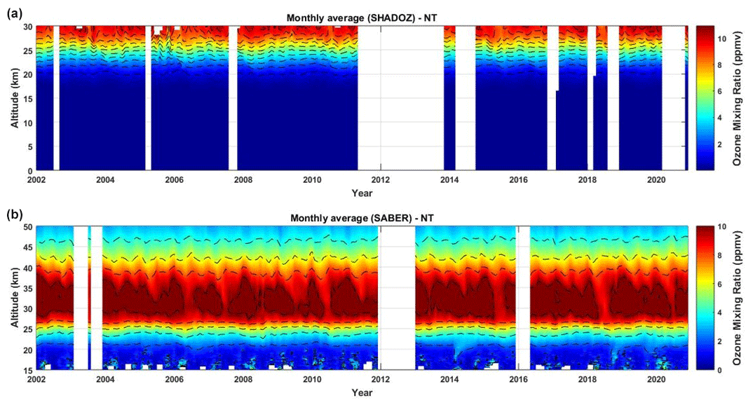
Figure 2 Time–height cross-section of monthly averages of ozone mixing ratio (in ppmv) over Natal (a) from radiosondes and (b) from the SABER instrument, respectively, in the 0–30 and 15–50 km altitude ranges, from January 2002 to December 2020.

3.1.1 SABER × SHADOZ comparisons in NT

Regarding the comparison between the two instruments, the relative differences were calculated, allowing the analysis of how the two databases (satellite and ozone soundings) behave in the tropical region over Brazil. In this way, due to the difference in the measures of the instruments, the analysis of coincident profiles was conducted, that is, profiles identified for the same days of analysis and the same region, in the 15–30 km altitude range, through the climatology of each time series. The first difference is in the vertical range of the two measurements. While SABER provides data between 15 and 110 km height, SHADOZ measurements are ranging from the surface up to 30 km height, approximately where the balloon bursts. Figure 3 displays the monthly climatological OMR profiles as derived from the two measurements over the NT station during the common observation period (2002–2020).

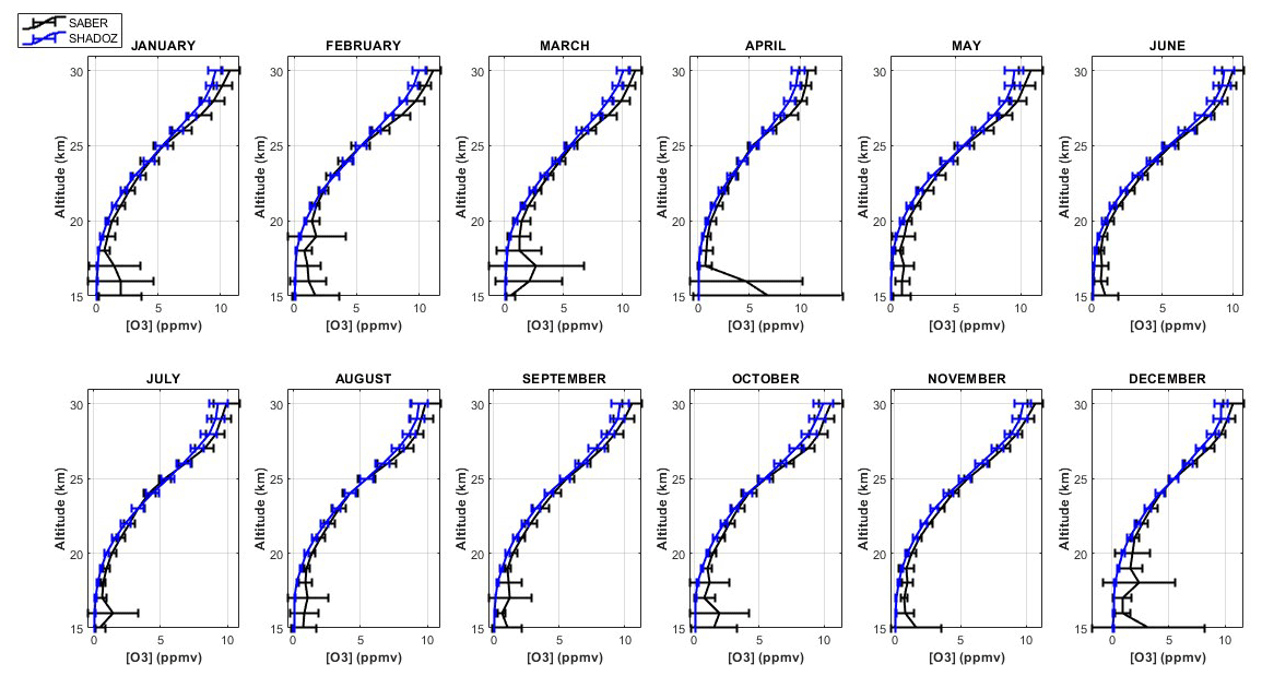
Figure 3 Monthly climatological OMR vertical profiles (in ppmv) as derived from SABER (black line) and SHADOZ (blue line) observations over Natal, between 15 and 30 km of altitude. The horizontal bars represent ±1σ (standard deviation).

The most evident differences are in the initial heights in relation to the SABER satellite (black lines). These could be explained mainly by divergences and errors in the boundary region of the satellite measurements (Fig. 3). These large differences below 20 km were also identified by Bahramvash et al. (2022). They reported large percentage differences between reanalysis data (MERRA-2), satellite profiles (AURA/MLS) and SHADOZ data, which show a good concordance mainly in the stratosphere between 22 and 34 km. Figure 3 shows that the most significant differences in OMR between the SABER and SHADOZ measurements appear in the UTLS region, between 15 and 20 km. These differences appear to be greatest during the summer and autumn, from December to April. In the middle stratosphere, between 20 and 26 km, the two OMR profiles (SABER in black and SHADOZ in blue) show similar behavior and begin to diverge in the upper stratosphere (beyond 26 km). This is probably due to the increasing uncertainty in the ozone measurement by SHADOZ as altitude increases. As a result, ozone at the top of SHADOZ profiles tends to be underestimated.

Some previous studies have examined ozone anomalies and variability using SHADOZ and SABER data for different regions of the world. For example, in southern Brazil (SM), Bresciani et al. (2018) performed a multi-instrument analysis to study an intense ozone depletion event in which the air mass came from the Antarctic ozone hole and influenced the region in 2016. The study compared satellite data, ground-based instruments, Brewer, and SHADOZ launched during the event. Toihir et al. (2018) identified long-term O₃ variability in the tropics and subtropics from January 1998 to December 2012, using TCO data from ground-based instruments, satellites, and vertical profiles through ozone soundings. The analyses were conducted at eight stations in the SH, including equatorial, tropical, and subtropical latitudes, and the results showed that the main variability that dominates the behavior of O₃ in the studied regions is the annual oscillation, with greater influence in the subtropics than in the tropics. Sivakumar et al. (2017) conducted a comparative study at the Irene site (25.9° S, 28.2° E), where they analyzed the climatological behavior of O₃ between the troposphere–stratosphere and its variability through data from SHADOZ and vertical profiles of O₃ from the AURA/MLS satellite. Based on the comparison of two instruments, they found that there were minor differences between SHADOZ and MLS ozone profiles. These differences were typically within ±10 % above 20 km. However, below 20 km, they found slightly larger differences, ranging from 15 % to 20 %. As seen from Fig. 3 there are significant differences in the UTLS region (below 20 km) between SHADOZ and SABER measurements at the NT site. To better quantify these differences, the OMR relative differences (RDs), as given in the previous section, were analyzed. Figure 4 illustrates these RDs in percentage for each month in the 20–30 km altitude range. The largest RDs occur in the lower stratosphere. On average, for altitudes above 22 km, RDs range from 5 % to 10 %, while the most significant differences are, as expected, obtained between December and April.

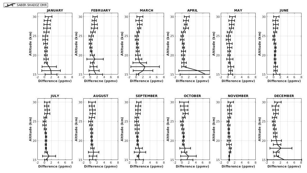
Figure 4 Profiles of percentage differences between monthly climatological OMR values from SHADOZ and SABER measurements over Natal station, from 2002 to 2020. The horizontal bars represent ±1σ (standard deviation).

3.2 O₃ vertical profile at subtropical and tropical latitudes

The comparison of the SABER satellite and SHADOZ data from Natal reveals good agreement between the two data series from altitudes higher than 20 km. We have therefore used SABER measurements to compare the vertical distributions of ozone over the two study sites, NT and SM, in the stratosphere, for altitudes ranging from 20 to 50 km. Figure 5 depicts the monthly climatological OMR derived over 19 years of SABER measurements over the subtropics at SM (blue line) and over the Equator at NT (black line). Comparison of the profiles indicates that the OMR climatological values are higher over Natal than over Santa Maria, particularly at altitudes ranging between 25 and 35 km. This is likely due to a greater ozone production resulting from photochemical reactions at the Equator than in the subtropics.

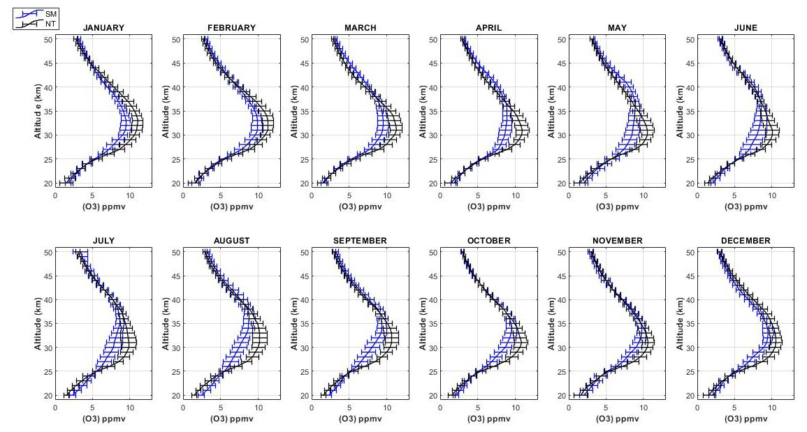
Figure 5 Comparison of monthly climatological OMR profiles between Santa Maria (blue) and Natal (black) using SABER data, during 2002–2020, between 20 and 50 km of altitude. The horizontal bars represent ±1σ (standard deviation). The monthly climatological OMR vertical profiles are given in parts per million by volume (ppmv).

This shows that the OMR varies according to latitude, altitude, and season of the year. As expected, this underlines its dependence on the intensity of incident solar radiation and the zenith angle (WMO, 2006; Seinfeld and Pandis, 2016). However, despite these factors for O₃ formation to occur at high altitudes at equatorial latitudes, the highest concentrations of O₃ are found at mid-latitudes and high latitudes, which is due to the large-scale air movement known as the Brewer–Dobson circulation (BDC) (Brewer, 1949; Dobson, 1930). The BDC transports O₃ from low latitudes, where it forms, to mid- and high-latitude regions. The balance between the O₃ production and destruction processes, in addition to being directly influenced by the amount of sunlight available in each region, also causes variations in the O₃ content as the air moves to different locations. Few studies have shown this difference between subtropical and tropical latitudes in South America in relation to the vertical variation of O₃. Sousa et al. (2020) compared total ozone columns over a tropical station (Cachoeira Paulista) and an equatorial station (Natal) using terrestrial and satellite data, presenting a trend analysis for Cachoeira Paulista and Natal. In fact, it has been established that O₃ production depends on factors such as latitude, altitude, and the season of the year. These factors explain why there are differences observed in O₃ distributions between regions where O₃ is generated and regions where it is transported. During the spring season, the ozone column is highest at mid-latitudes around 45° N in the Northern Hemisphere and from 45 to 60° S in the Southern Hemisphere. However, during winter, ozone abundance in equatorial regions is lower than in polar regions (Holton, 1995; Gettelman et al., 2011). The O₃ maxima in spring are due to the increased transport of ozone from the tropics to the mid-latitudes and high latitudes in late autumn and winter. This is due to the BDC, which tends to accelerate in the context of climate change (Neu et al., 2014), with impacts on ozone distributions at different latitudes.

From the ozone time series obtained from SABER measurements over the study period, it is possible to extract monthly series of ozone mixing ratio (OMR) by altitude and the associated climatological variations. Figures 6 and 7 depict the monthly and climatological variations of OMR in the stratosphere at altitudes of 24, 32, 40, and 48 km, over the two study sites, SM (blue lines) and NT (black lines). At 24 km, the two latitudes are influenced by dynamic processes in the lower stratosphere. However, for most of the heights, the two stations appear to be almost in opposition phase, which can be explained by the different dynamic forcings at each region, such as the quasi-biennial oscillation (QBO) showing a direct influence at tropical latitudes impacting stratospheric ozone chemical and dynamic processes (Anstey and Shepherd, 2014; Naoe et al., 2017). At this altitude, one can also observe, from Fig. 7a, that the two sites exhibit different climatological behaviors. A well-marked annual cycle is observed at SM, with maxima in winter and minima in summer months. At the same time, in NT, the behavior of O₃ is more constant, without much variation in OMR, which could be related to the effect of transport induced by the BDC (Butchart, 2014). At the height of 32 km, ozone is expected to be more controlled by photochemical processes than dynamics. Figure 6b aligns with this. It shows that at 32 km height, the OMR above Natal (equatorial region) consistently remains higher than that above Santa Maria (subtropics). The monthly climatology shows the influence of the seasons, where the maximum values of OMR (9.5–12 ppmv for NT and 8–10 ppmv for SM) occur during austral summer and minimum values of OMR (9–11 ppmv for NT and 7–9 ppmv for SM) during austral winter. The high altitudes are shown in Fig. 7c for 40 km and Fig. 7d for 48 km. At 40 km, the semi-annual cycle seems to prevail at NT, while the annual cycle tends to dominate at SM. In comparison, at 48 km, OMR over SM also shows a semi-annual trend. The observed variability of ozone is mainly due to the combined effect of its production in tropical regions and its transport to mid-latitude and polar regions. Sousa et al. (2020) showed that Cachoeira Paulista and NT present maximum values in spring regarding the seasonality of O₃ content in both seasons, with a well-established annual cycle, in agreement with the results found in the present work.

Figure 6 Time series of monthly mean OMR at 24 km (a), 32 km (b), 40 km (c), and 48 km altitude (d), as derived from SABER measurements over Santa Maria (blue) and Natal (black) (in ppmv).

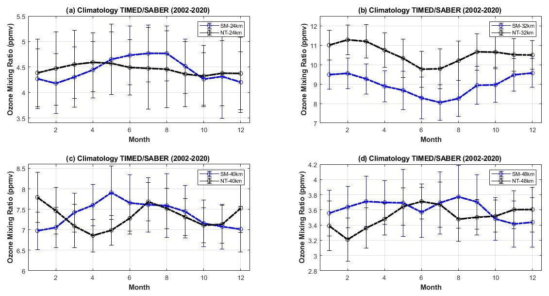
Figure 7 Monthly climatological OMR values (in ppmv) for SM (in blue) and NT (in black) from SABER records from 2002 to 2020 at four selected heights: (a) 24 km, (b) 32 km, (c) 40 km, and (d) 48 km. The vertical bars represent ±1σ (standard deviation).

3.3 Total column ozone in subtropical and equatorial latitudes

This subsection examines the TCO time series obtained for the two study sites, NT and SM. The TCO time series construction is described in Sect. 2.1.3.

Figure 8 shows the daily (SM) and monthly (NT) TCO values from ground-based and satellite instruments. There is a well-defined annual cycle in all TCO data sets. In addition, the comparison between the instruments shows a good agreement. Toihir et al. (2018) analyzed satellite data and ground instrument trends and changes in O₃ at tropical and subtropical latitudes in the Southern Hemisphere. One of their results showed a good correlation between the instruments, which showed that they were used correctly, mainly satellite data for O₃ content analysis. Vaz Peres et al. (2017), for subtropical latitudes, and Sousa et al. (2020), for equatorial latitudes, showed a good correlation in TCO data for a shorter period of data, indicating good agreement between satellite and ground-based data in southern Brazil.

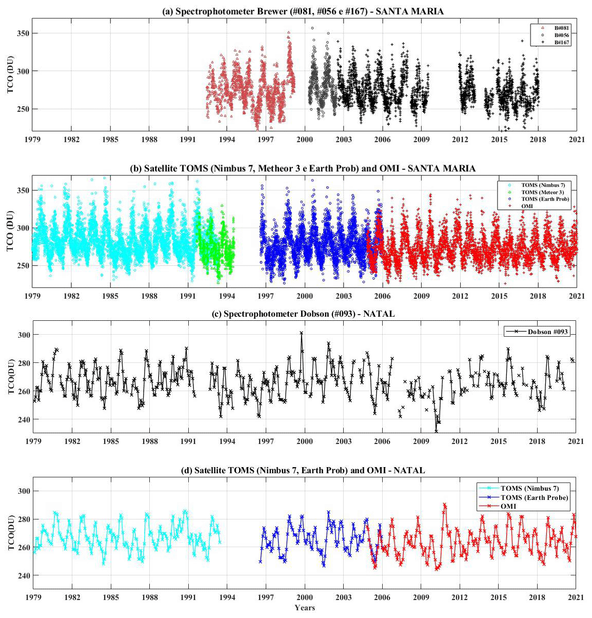
Figure 8 Time series for 1979–2020 of the daily-average TCO for Santa Maria with Brewer data (a) and satellite data (TOMS and OMI) (b). Natal showing Dobson data (c) and satellite data (TOMS and OMI) (d).

A comparative statistical analysis was performed based on the difference between ground-based and satellite instruments. The SM data series are presented (Brewer vs. TOMS) from June 1992 to December 2005, containing 2164 pairs of data (daily), and between October 2004 and December 2017 (Brewer vs. OMI), with 4621 pairs of data. In SM, each data set represents the monthly series of each instrument. It is observed that the correlation coefficient (R²) concerning the instruments presented considerably good values, where the values of the correlation coefficient were 0.88 (Brewer vs. TOMS) and 0.92 (Brewer vs. OMI). Improvements in satellite equipment over the years may explain this good correlation between TOMS and OMI. Regarding data from TOMS and OMI satellites, previous studies have shown similar results concerning comparisons between these TCO measurement instruments over different regions. Antón et al. (2009) compared data from the OMI satellite with different ground-based instruments in the Iberian Peninsula and identified a good correlation between the instruments and the behavior of the TCO. Toihir et al. (2015) analyzed the average monthly behavior of the TCO at 13 locations in tropical and subtropical latitudes, comparing satellite data from the EUMETSAT program and OMI and ground-based data from the SAOZ and DOBSON spectrometers available at these stations; the results found showed good correlations between these instruments, with values around 0.87.

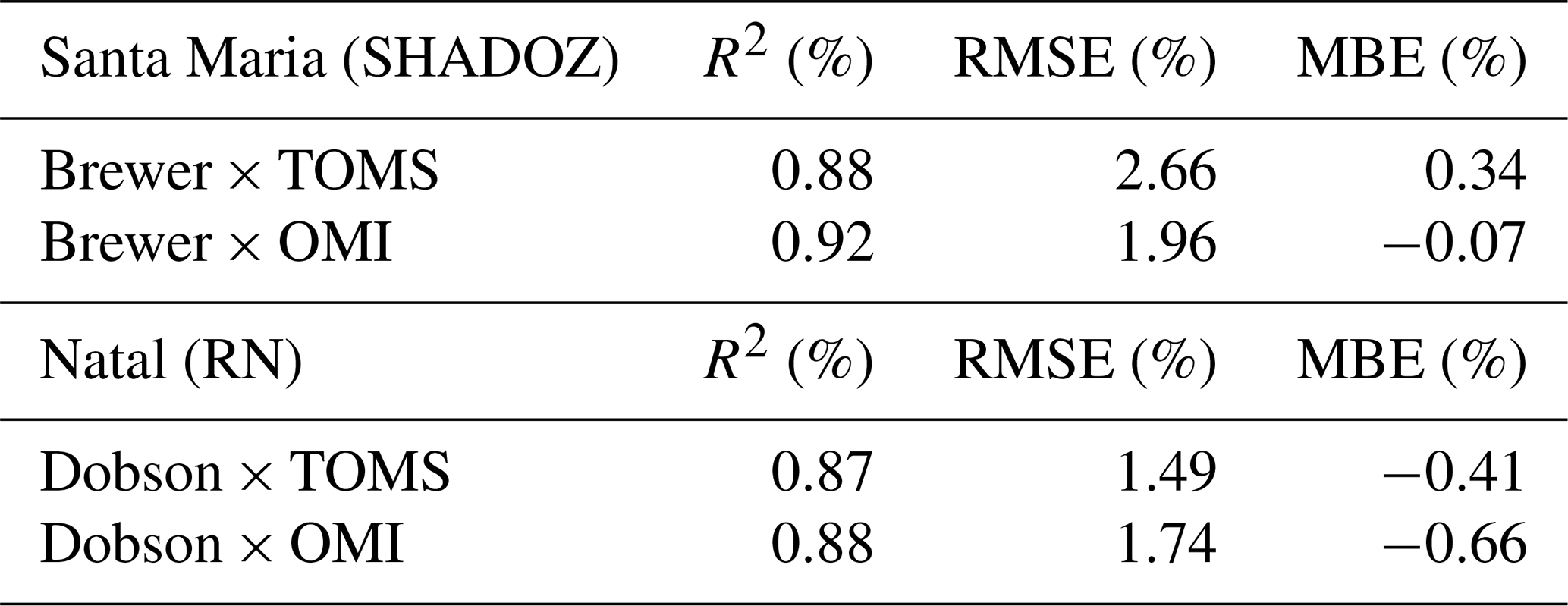
The root mean square error (RMSE) showed less than 3 % difference in all data sets, which is coherent with the high correlation values between the instruments presented above. The mean bias error (MBE) in the analysis of the daily TCO data showed an overall overestimation of the TOMS measurements (0.34) and an underestimation of the OMI satellite data (−0.07) in comparison with the Brewer measurements, as reported in Table 1. These results confirm the effectiveness of TCO measurements at the subtropical station of Santa Maria during the 42 years of data studied in this work, agreeing with previously presented works that perform similar analyses. Vaz Peres et al. (2017) showed a good correlation in TCO data for a shorter period of data, indicating a good agreement between satellite and ground-based data in the southern region of Brazil. In this work, during the period 1979–2020 in NT, the coefficient of determination (R²) between Dobson vs. TOMS was 0.87, and in the comparison between Dobson and OMI, the R² found was 0.88. For Natal, the RMSE values were 1.49 % for the DOBSON vs. TOMS comparison and 1.74 % for DOBSON vs. OMI; these agree with results reported by Sousa et al. (2020), who identified values around 2.81 % considering TOMS data and 1.94 % with OMI. For the MBE values, it was observed that both TOMS and OMI underestimate the values of the Dobson spectrophotometer, presenting negative values of −0.41 % (TOMS) and −0.66 % (OMI).

Table 1 summarizes the R², RMSE, and MBE values for comparing the TCO series in SM and NT. Sousa et al. (2020) presented similar comparison values for the period 1974/1978–2013 for equatorial and tropical latitudes, with R² values around 0.83 % (DOBSON vs. TOMS) and 0.91 % (DOBSON vs. OMI). These high coefficients of determination indicate improvements in the new generation of satellites (the replacement of TOMS by OMI in 2005).

Table 1 Statistical analysis between ground-based instruments (Brewer and Dobson) and satellites (TOMS, OMI) for Santa Maria and Natal between 1979–2020.

3.3.1 TCO climatology

The monthly climatological TCO values and the associated standard deviation are presented in Fig. 9 for the subtropical station in SM (blue) and the equatorial station in NT (black) based on data collected from 1979 to 2020. Previous work has highlighted the annual variability in the TCO to SM series, with minimum values in autumn (April and May) of between ∼ 255 and 260 DU and maximum values during the austral spring (September and October) of between ∼ 295 and 300 DU (Vaz Peres et al., 2017; Bittencourt et al., 2019). For the NT station, one can identify a well-established annual cycle with minima during autumn, ranging from 255 DU in May to 280 DU in September–October when it reaches its maximum peak. These results agree with Bencherif et al. (2024) and Sousa et al. (2020), who identified an annual cycle over the NT equatorial latitude. This variability with minima in autumn and maxima during spring could be explained by the large-scale transport due to the BDC. This transport implies that the O₃ produced in low latitudes is transported to mid- and high-latitude regions, causing this maximum to occur during the end of winter and beginning of spring (London et al., 1985). Furthermore, in this region, tropospheric O₃ is also influenced by biomass burning, which considerably increases its O₃ content during spring, peaking in October (du Preez et al., 2021).

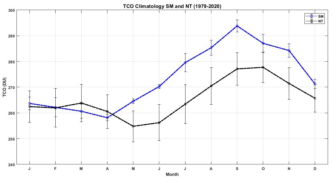
Figure 9 Monthly climatology for SM (blue) and NT (black) of the TCO in DU during the period 1979 to 2020. The vertical bars represent ±1σ (standard deviation).

Sivakumar et al. (2007) conducted a study on the climatology and stratospheric ozone variability over Reunion Island (a tropical site), from 15 years of data available from satellite instruments (HALOE, SAGE-II, TOMS) and ozonesondes; they also identified maximum O₃ values during spring and minimum values during autumn. Vaz Peres (2017) identified a similar behavior in analyzing O₃ content at Santa Maria, south of Brazil, at the Southern Space Observatory. Santos (2016) showed the stratosphere–troposphere exchanges (STEs) for southern Brazil, where a greater number of exchanges was identified during the winter and spring months, with a lower frequency during the summer, also explained by the BDC.

At NT, comparisons between instruments (DOBSON vs. TOMS, DOBSON vs. OMI) were satisfactory for the tropical region, showing that satellite and ground-based measurements agree with previous works. Toihir et al. (2018) analyzed the trend and variability of O₃ content in eight locations in equatorial, tropical, and subtropical latitudes, comparing data from satellite, ground-based instruments, and ozonesondes through the SHADOZ network. The comparison between the instruments for the period from 1998 to 2012 showed good agreement, and SHADOZ vertical profile data were considered of good quality to study and identify the main variables in addition to the trend behavior of the O₃ content with this database and well-established data for the equatorial, tropical, and subtropical regions.

3.3.2 Variabilities in subtropical and equatorial latitudes

The wavelet transform makes it possible to indicate the main forcing cycles and components contained in a signal (ozone series in our case) and their evolution over time. For SM and NT, the wavelet analysis was applied to the monthly anomaly series of the TCO for both stations. Figure 10 presents the set of wavelet analysis for Santa Maria (Fig. 10a) and Natal (Fig. 10b) for the 42 years (1979–2020). In all analyses, the seasonal variability was removed. The white contours include regions with a confidence level greater than 95 %, and the U-shaped curve indicates the cone of influence. The cone of influence is a numerical parameter used in wavelet analysis to define the region of the spectrum which should be considered in the analyses with confidence. It indicates areas where edge effects occur in the analyzed time series. (Torrence and Compo, 1998; Loua et al., 2019).

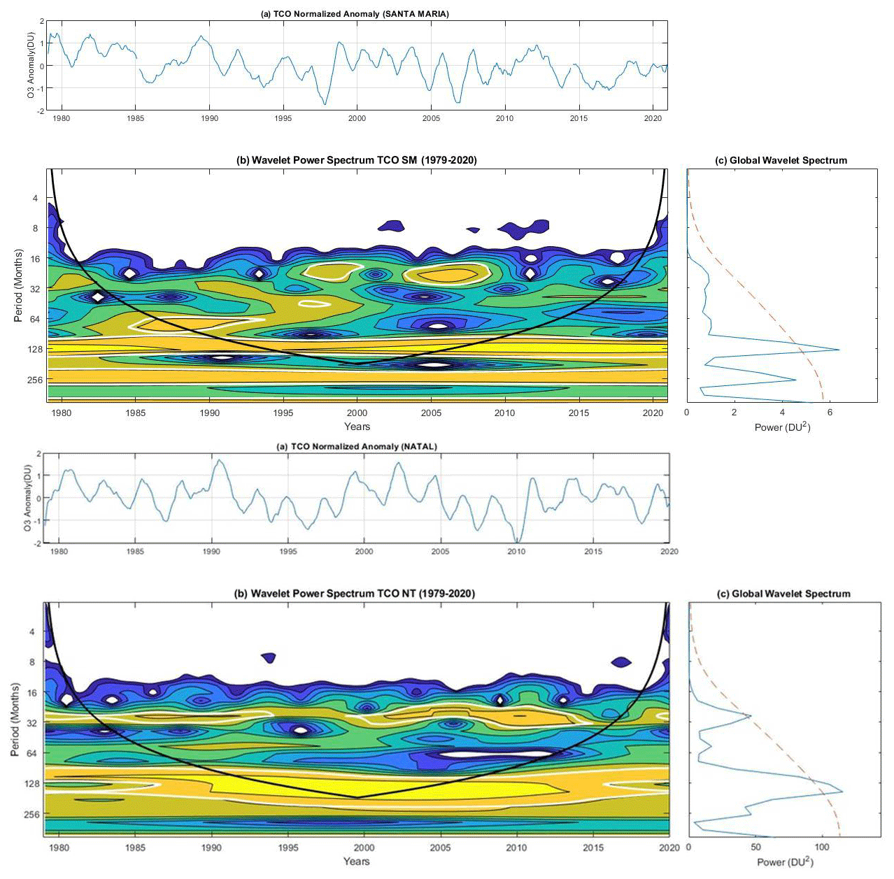
Figure 10 Morlet wavelet power spectrum, normalized by (1/σ²) of the TCO anomaly time series at Santa Maria (a) and Natal (b). The TCO anomaly time series is shown in the panel above the power spectrum, while the global wavelet spectrum is given on its right.

In the power spectrum for the two latitudes analyzed, in the range of 132 months and the 11-year solar cycle, there is an important variability for ozone in the subtropical and equatorial regions of South America. More intense variability is also observed between 16–32 months, mainly for NT, which had a strong influence on the TCO data series in equatorial latitudes, with greater intensity within the cone of influence from 1983 to 1995 and between 2000 and 2015. This strong variability makes it possible to indicate the strong presence of the quasi-biennial oscillation (QBO) in this region. Naoe et al. (2017) analyzed the future of the QBO in ozone in the tropical stratospheric region, through simulations related to the increase in the greenhouse gases and the decrease in O₃-destroying substances, identifying a maximum in the amplitude of the QBO between 5–10 hPa and suggesting that, at this time, the photochemistry of the region will depend on temperature to modulate ozone in the tropical stratosphere. Newman et al. (2016) showed an anomalous QBO phase shift over the past 60 years. The anomaly showed a rapid upward shift from the westerly phase of the equatorial winds to an easterly phase between 2015–2016. This sudden QBO phase change resulted in the shortest east phase ever seen in records from 1953 to 2016. In this way, ozone's response to changes in solar irradiation also plays a potentially important role in climate change, regulating stratospheric temperatures and winds. These changes in the stratosphere can affect tropospheric climate through direct radiative effects and dynamic coupling, affecting patterns of extratropical variability (WMO, 2018). Changes in the BDC also modulate the behavior of ozone in the stratosphere, both by its transport, which is influenced by the strongest and/or weakest impulse in the tropics, and by the chemistry in the formation of O₃ at tropical latitudes (WMO, 2022).

Despite having a low frequency for the subtropics (SM), this QBO signal was observed at a lower frequency than NT and in other studies at subtropical latitudes (Rigozo et al., 2012; Toihir et al., 2018). Figure 10b shows the behavior of the TCO time series at Natal from 1979 to 2020. With a periodicity ranging from 24 to 32, the QBO appears to appear to be one of the main forcings of ozone at Natal. In fact, many previous studies showed that the QBO and the solar cycle are among the most dominating variability of O₃ in tropics (Baldwin, 2001; Salby and Callaghan, 2002). Moreover, studies have shown that the QBO and solar cycle forcings are mainly important and dominant in the stratosphere than in the troposphere (Bencherif et al., 2024). To highlight this, we applied the same wavelet analysis to a stratospheric OMR time series (24 km) at both sites, NT and SM. Figure 11 depicts the set of wavelet analysis at 24 km for SM (Fig. 11a) and NT (Fig. 11b) using SABER OMR data. The influence of the QBO appears to be evident at NT (Equator) but less evident for SM (subtropics). Vaz Peres et al. (2017) reported that there is a phase opposition between the QBO modulation and the TCO anomalies obtained for the SM site over the period 1992–2014. In addition, from Fig. 11, it should also be noted that the ENSO cycle (El Niño–Southern Oscillation) appears to have little impact on O₃ variability at both sites. This is in agreement with the finding from Toihir et al. (2018).

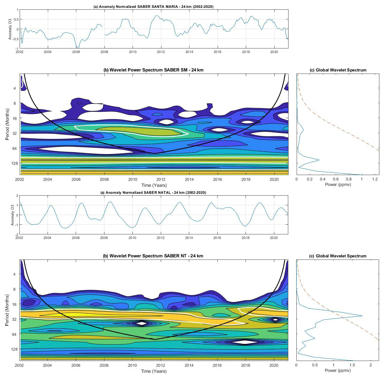
Figure 11 Same as Fig. 10, but the wavelet analysis is for the SABER OMR time series at 24 km height for Santa Maria (a) and Natal (b) over the 2002–2020 period.

When the multilinear regression model, Trend Run, is applied to the 24 km OMR time series for both sites, we obtain a higher contribution from the QBO at the Equator (Natal), of the order of 37.6 % ± 0.2 %, whereas this contribution is much lower at Santa Maria (of the order of 2.8 % ± 0.04 %). As for the percentage contribution of the ENSO cycle to stratospheric ozone variability, it shows a lower contribution than the QBO but with an opposite situation, a greater contribution in Santa Maria (∼ 2.8 % ± 0.04 %) than in Natal (∼ 1.59 % ± 0.04 %). This agrees with the results obtained using wavelet analysis (Fig. 11). This is also consistent with the findings of Toihir et al. (2018), who reported that the influence of ENSO on ozone is weak and accounts for around 1 % to 2 % in the equatorial stratosphere. Given the relatively small size of the analyzed OMR times series (19 years), the solar cycle contributions estimated by the Trend Run model are small (less than 0.5 %) and insignificant. They cannot therefore be discussed.

4 Conclusions

This work describes the behavior of ozone content through a multi-instrumental analysis for two different latitudes in Brazil, Santa Maria (29.4° S, 53.8° W) comprising subtropical latitudes and Natal (5.4° S, 35.4° W) representing the equatorial region of Brazil, through the analysis of the vertical profile data in the period of 19 years of data (from 2002 to 2020) and analysis of the total column ozone (TCO) for the two stations between 1979 to 2020, in order to identify the main climatic variables that influence O₃ at both latitudes. Vertical profile data were obtained by the TIMED/SABER satellite, and to compare these data, ozonesondes were also analyzed through the SHADOZ measurement network at the Natal station. For the TCO data series, satellite data (TOMS and OMI) and ground-based data (Brewer and Dobson spectrophotometers) from instruments installed and operating in Santa Maria and Natal, respectively, were used.

Comparative studies between satellite data (SABER) and ozonesondes from the SHADOZ network in Natal showed that the most significant relative differences between the two databases are below 20 km altitude, for the most part. These differences, between 15 and 20 km, can be explained by inconsistencies of the satellites, not representing the UTLS region measurements very well since the SABER satellite starts its analysis around 15 km altitude. On the other hand, above 22 km, the differences are relatively smaller, varying by less than 20 % in most months in the comparison between the two instruments (SABER and SHADOZ), and therefore, vertical profiles of the SABER satellite can carefully represent the behavior of O₃ for the latitudes that are being studied in this work. These results showed that studies using data from the SABER satellite to analyze the lower stratosphere, below 20 km altitude, are not a good option for Natal station. Furthermore, few studies compare stations at different latitudes in South America regarding the analysis of vertical O₃ content using data provided by satellites. On the other hand, studies that monitor the TCO also present good comparative results between different measuring instruments for different latitudes.

TCO and stratospheric ozone levels tend to remain steadier and vary with latitude. This highlights the significance of establishing stratospheric ozone measurement stations in regions beyond equatorial and tropical latitudes, especially in the Southern Hemisphere. The SM site is an excellent location to participate in this mission of monitoring and observing stratospheric ozone since the site often experiences AOH events. Additionally, there are no long-term ozone profiling stations at this latitude or nearby in the SH.

The latitudinal differences of the study regions show different behavior of the ozone content. For example, the altitude of 24 km for both Santa Maria and Natal is influenced by dynamic processes in the lower stratosphere region, where each region has an important characteristic dynamic forcing in this variation. At altitudes between 32 and 40 km, the photochemical factor controls the O₃ content at both latitudes in the middle and upper stratosphere. An annual variation stands out at both latitudes, mainly at 32 km altitude, with maxima during spring–summer and minima in autumn–winter due to the low incidence of radiation. The small amount of ozone at altitudes such as 48 km could explain the little variation during the year for subtropical latitudes (Santa Maria).

Using TCO data from satellites and terrestrial instruments, it is possible to indicate the climate variability that stands out for both latitudes, where the data showed a strong influence of the solar cycle in subtropical and equatorial latitudes. The annual cycle is also a dominant variability in the TCO series in Santa Maria, as observed in the climatological analyses. In the equatorial latitudes of Natal, in addition to the solar cycle, the other influence that can be observed is the QBO, which modulates the behavior of O₃ in the tropical region where the main photochemical processes occur in the formation of ozone gas. Changes in this oscillation (QBO) can interfere with the dynamics of the large-scale movement of the Brewer–Dobson circulation, modulating the distribution of O₃ to other regions.