the Creative Commons Attribution 4.0 License.
the Creative Commons Attribution 4.0 License.
 | 06 Sep 2024
Assessing the potential of free-tropospheric water vapour isotopologue satellite observations for improving the analyses of convective events
Matthias Schneider
Kinya Toride
Farahnaz Khosrawi
Frank Hase
Benjamin Ertl
Christopher J. Diekmann
Kei Yoshimura
Satellite-based observations of free-tropospheric water vapour isotopologue ratios (HDO H2O, expressed in form of the δ value δD) with good global and temporal coverage have become available recently. We investigate the potential of these observations for constraining the uncertainties of the atmospheric analyses fields of specific humidity (q), temperature (T), and δD and of variables that capture important properties of the atmospheric water cycle, namely the vertical velocity (ω), the latent heating rate (Q2), and the precipitation rate (Prcp). Our focus is on the impact of the δD observations relative to the impact achieved by the observation of q and T, which are much more easily observed by satellites and are routinely in use for atmospheric analyses. For our investigations we use an Observing System Simulation Experiment; i.e. we simulate the satellite observations of q, T, and δD with known uncertainties and coverage (e.g. observations are not available for cloudy conditions, i.e. at locations where the atmosphere is vertically unstable). Then we use the simulated observations within a Kalman-filter-based assimilation framework in order to evaluate their potential for improving the quality of atmospheric analyses. The study is made for low latitudes (30° S to 30° N) and for 40 d between mid-July and the end of August 2016. We find that q observations generally have the largest impacts on the analyses' quality and that T observations have stronger impacts overall than δD observations. We show that there is no significant impact of δD observations for stable atmospheric conditions; however, for very unstable conditions, the impact of δD observations is significant and even slightly stronger than the respective impact of T observations. Very unstable conditions are rare but are related to extreme events (e.g. storms, flooding); i.e. the δD observations significantly impact the analyses' quality of the events that have the largest societal consequences. The fact that no satellite observations are available at the location and time of the unstable conditions indicates a remote impact of δD observations that are available elsewhere. Concerning real-world applications, we conclude that the situation of δD satellite observations is very promising but that further improving the model's linkage between convective processes and the larger-scale δD fields might be needed for optimizing the assimilation impact of real-world δD observations.
- Article
(4504 KB) - Full-text XML
- BibTeX
- EndNote


Clouds and water vapour control atmospheric radiative heating and cooling, and the condensation or evaporation of water determines where latent heat is released or consumed. The heating patterns then drive the atmospheric circulation, whereby in particular vertical transport causes additional evaporation/condensation and impacts the distribution of water vapour and clouds, which in turn again modifies the latent and radiative heating patterns of the atmosphere. This strong coupling between moisture pathways, diabatic heating, and atmospheric circulation is responsible for important climate feedback mechanisms (e.g. Sherwood et al., 2014; Bony et al., 2015) and is often connected to the evolution of severe weather events (e.g. Fink et al., 2012; Evans et al., 2017). In this context, it is rather worrisome that the diabatic heating rates and the related vertical transport obtained from different current global reanalyses show significant inconsistencies (e.g. Chan and Nigam, 2009; Ling and Zhang, 2013).
For the generation of daily- and global-scale analyses, the operational assimilation systems assimilate the outgoing microwave or infrared radiation (e.g. Eyre et al., 2022). This radiation contains information on the atmospheric state (mostly atmospheric specific humidity, q, and temperature, T). There are many different satellites that measure this radiation in a spectrally resolved manner, including operational weather satellites, like the European Meteosat and Metop series (https://www.eumetsat.int/our-satellites/meteosat-series, last access: 2 September 2024, and https://www.eumetsat.int/our-satellites/metop-series, last access: 2 September 2024, respectively).
In this study, we investigate the information that free-tropospheric δD observations can offer in addition to the information provided by the observations of q and T for improving the analyses.
The δD value is calculated as the ratio between the D and H isotopes in water vapour relative to a standard ratio:
where H2O and HDO are the concentrations of all the isotopologues containing two H isotopes and one H and one D isotope, respectively. The Vienna Standard Mean Ocean Water ratio of the two isotopologues (RVSMOW = 3.1152 × 10⁻⁴) is a standard ratio typically encountered in ocean water. The reason that δD is of particular interest is that, firstly, it can be observed with a reasonable precision by satellites on a daily and almost global scale (e.g. Diekmann et al., 2021b), and, secondly, HDO enrichment or depletion contains information on vertical transport and convective processes. For vertical or horizontal mixing between dry/depleted and humid/enriched water masses, HDO tends to be enriched (Noone et al., 2011; González et al., 2016). Conversely, recurring evaporation and condensation in the context of convective activity cause a strong HDO depletion (e.g. Bony et al., 2008; Risi et al., 2008; Noone, 2012; Field et al., 2014; Galewsky et al., 2016; Diekmann et al., 2021c).
During the last 15 years, tropospheric δD products have been developed for different satellite sensors (e.g. Worden et al., 2007; Frankenberg et al., 2009; Schneider and Hase, 2011; Lacour et al., 2012; Boesch et al., 2013; Worden et al., 2019; Schneider et al., 2020). Meanwhile, different weather and climate models have the water isotopologues and the relevant physical processes implemented and can provide modelled isotopologue fields on a global and regional scale at different horizontal resolutions (e.g. Yoshimura et al., 2008; Risi et al., 2010; Werner et al., 2011; Pfahl et al., 2012; Eckstein et al., 2018; Tanoue et al., 2023). This offers advanced opportunities for studying atmospheric moisture processes with water isotopologues.
The tropospheric water vapour isotopologue composition has been used for investigating water-cycle-related biases in atmospheric models (e.g. Risi et al., 2012; Field et al., 2014; Schneider et al., 2017), processes involving clouds or precipitation (e.g. Webster and Heymsfield, 2003; Worden et al., 2007; Blossey et al., 2010; Field et al., 2010; Bailey et al., 2015; Diekmann et al., 2021c), local diurnal-scale moisture transport (Noone et al., 2011; González et al., 2016), and large-scale moisture transport (e.g. Noone, 2012; González et al., 2016; Lacour et al., 2017; Dahinden et al., 2021).
We use a data assimilation framework together with an OSSE (Observation System Simulation Experiment) to document the added value of the free-tropospheric δD satellite observations; i.e. we simulate satellite observations and then evaluate the theoretical impact of assimilating the observations. This assimilation framework was presented in Yoshimura et al. (2014) and has already been applied by Toride et al. (2021) and Tada et al. (2021). Here we simulate the observations in line with the temporal and horizontal coverage achieved by the IASI (Infrared Atmospheric Sounding Interferometer; Clerbaux et al., 2009) satellite sensor. We simulate the IASI data of q, T, and δD as generated for the free troposphere using the retrieval processor MUSICA (MUlti-platform remote Sensing of Isotopologues for investigating the Cycle of Atmospheric water; Schneider et al., 2016, 2022). We evaluate the analyses of the atmospheric fields of q, T, δD, the vertical velocity (ω), the latent heating rate (Q2), and the precipitation rate (Prcp). The latter three are strongly coupled and linked to climate feedbacks and weather events. The atmospheric dynamics (expressed among others by ω) is coupled to Q2, which in turn affects the vertical thermal structure and thus dynamics. Prcp describes the removal of moisture from the atmosphere, which in turn affects the Q2 and radiative heating potential.
This study is complementary to Toride et al. (2021), where observations from different platforms and different temporal and spatial coverages were used (satellite, radiosonde, and surface observations). The different observational techniques provide diverse information; however, using observations that have a spatial and temporal coverage that differs from the coverage of the IASI δD data makes it difficult to understand whether an improvement in the analysis is due to the complementarity of the information provided by δD or the complementary coverage (the coverage of IASI δD is much better than the coverage of radiosonde data and more homogeneous than the coverage of the surface data and data from geostationary satellites; see Figs. S4 and S5 in the Supplement of Toride et al., 2021). In our OSSE, all observations have the same spatial and temporal coverage (the coverage of the MUSICA IASI water isotopologue satellite data; Diekmann et al., 2021b), which ensures that any improvement in the analysis by an additional assimilation of δD is due to the complementarity of the information provided by δD and not due to different coverages. Furthermore, we investigate the assimilation of δD in addition to the assimilation of satellite observations of q and T. The latter (i.e. IASI observations of T) were not considered in Toride et al. (2021), despite the fact that they are available with good quality. Moreover, in addition to the general impact study given by Toride et al. (2021), this work investigates the situations when the isotopologue observations can make a unique contribution (versus the situations when they have no significant impact).
In Tada et al. (2021) real IASI δD observations (only δD observations) were assimilated, and it was shown that such assimilation leads to a better agreement with the ERA5 reanalyses (Hersbach et al., 2020) than not assimilating any data. However, they did not investigate the much larger impact that can already be achieved by assimilating more easily observable data like q and T. In this context, our study has a very different focus: we use the assimilation of the easily observable data (q and T) as the reference and evaluate the impact of additionally assimilating δD observations.
The paper is structured as follows: Sect. 2 describes the simulated data and the OSSE, the performed assimilation experiments, and the analysed atmospheric variables, as well as the methods used for evaluating their quality. In Sect. 3, we give an overview on the analyses' quality improvements achieved by the different assimilation experiments. Section 4 examines for what atmospheric conditions the δD observations have the strongest impact on the analyses, and it briefly discusses some challenges that have to be overcome for achieving an optimal δD assimilation impact for real-world analyses. A summary of the study is given in Sect. 5.
2.1 Data simulations
We use the isotopologue-enabled atmospheric general circulation model IsoGSM (Yoshimura et al., 2008) and simulate the atmospheric state for the 2 months of July and August 2016, in 6 h time steps, with a spectral model grid resolution T62 (about 200 km horizontal resolution and 28 vertical sigma levels). We use this simulation as the truth and refer to it in the following as the nature data (, where the index i indicates the time step and the index j the location).
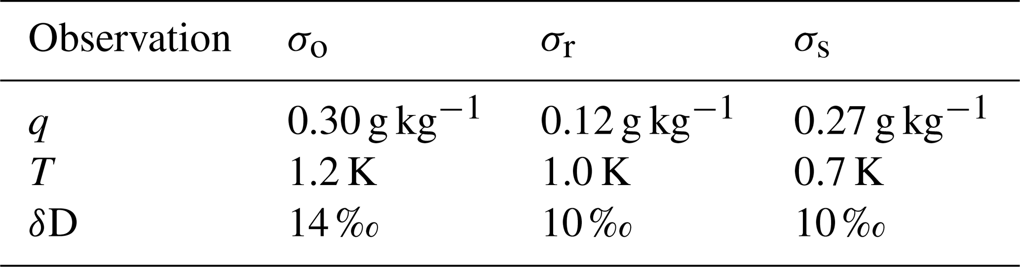
For our OSSE we consider that a thermal infrared sensor like IASI offers no free-tropospheric trace gas products in the presence of mid- and high-level clouds, so we limit the observational data availability to time steps and locations where the model is free of mid- and high-level clouds. Furthermore, we take into account IASI's high horizontal resolution (ground pixel diameter of about 12 km at nadir), which is much finer than the 200 km horizontal resolution of IsoGSM. Typically there are about 10–20 high-quality MUSICA IASI observations each 12 h in the 200 × 200 km area, which is represented by IsoGSM (Diekmann et al., 2021b). We simulate MUSICA IASI observations of q, T, and δD in the middle troposphere (at about 550 hPa) and consider the different horizontal representations of the model and observations when setting up the observational error variance (). For this purpose, we estimate as the sum of a spatial representativeness error variance () and a retrieval error variance (). The σr value is the mean error estimated for the MUSICA IASI data within a IsoGSM grid box (it is typically 0.12 g kg−1, 1.0 K, and 10 ‰ for q, T, and δD, respectively; Diekmann et al., 2021b). For the σs values we use the standard deviations of the MUSICA IASI data within the IsoGSM grid box, which is generally of a similar order as σr. Table 1 gives a summary of the typically assumed observational errors.
Table 1Summary of the typical free-tropospheric observational error (σo) used for the assimilation experiments. The σo values are calculated as the root square sum of MUSICA IASI retrieval noise error (σr) and the spatial representativeness error (σs), due to resampling the small MUSICA IASI ground pixels onto the relatively coarse 200 × 200 km IsoGSM grid.
In addition to the nature data, the data belonging to the different ensemble members have to be simulated. This is done with IsoGSM but with initializations from different time steps within the same season of the nature run. These initial conditions are considered independent from the nature run (for more details, see Toride et al., 2021). We calculate an ensemble with 96 members (i.e. Nens = 96).
2.2 Data assimilation with a Kalman filter
For the data assimilation we use the local ensemble transform Kalman filter (LETKF; e.g. Hunt et al., 2007) method as developed for its use with water isotopologue data by Yoshimura et al. (2014). The Kalman-filter-based data assimilation technique optimally combines a model forecast with an observation by considering the respective model and observational uncertainties (Kalman, 1960). The result is a best estimate of the atmospheric state (the analysed state vector, xa):
where xb is the so-called background state (the model forecast), y the observation vector, and H the observational operator (a matrix operator which maps the model state into the observation space). The matrix operator K is the Kalman gain:
where the first and second line are the so-called m and n forms, respectively (whose equivalence is shown, for instance, in Chap. 4 of Rodgers, 2000). The matrix B is the uncertainty covariance of the background state (it is calculated as the covariance of the different ensemble runs and thus captures the uncertainty of the model forecasts). In the following, its inverse (B−1) is also referred to as the background knowledge information matrix (it is a measure for the knowledge about the atmospheric state, including the statistical dependency of different atmospheric state variables). The matrix R is the uncertainty covariance of the observational state (it captures the uncertainties of the observations). In Eq. (2), if we substitute K by the second line of Eq. (3) and y by Hx (the observation y is the actual atmospheric state x mapped to the observational domain), we get
which reveals that the Kalman filter weights the impact of the background and the observation on the analyses reciprocally according to their respective uncertainties. More details on the LETKF settings used, like the localization, the covariance inflation, or the ensemble size choice, are given in Sect. S2 of the Supplement of Toride et al. (2021).
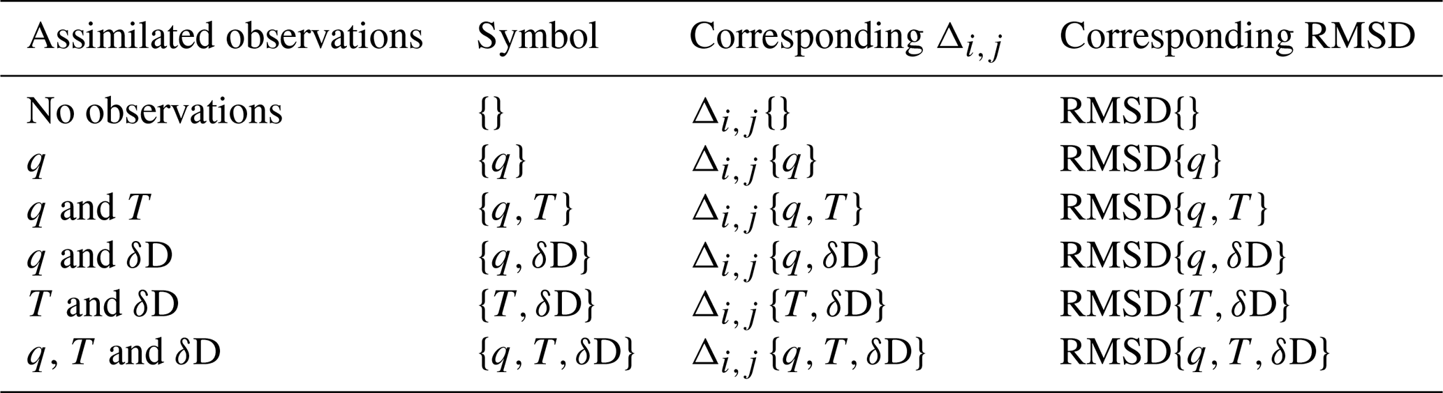
Our assimilation experiments use observations of specific humidity (q), atmospheric temperature (T), and the isotopologue ratio of water vapour (δD) at about 550 hPa, which is the pressure level where the MUSICA IASI products generally have a very good quality (high sensitivity and low uncertainty). An overview of the different assimilation experiments performed is given by Table 2.
Table 2Summary of the different assimilation experiments used in this study. The column “Assimilated observations” lists the observations used for the experiment; the column “Symbol” shows the symbol used in the following when referring the respective experiment; the column “Corresponding Δi,j” shows the symbol used for the corresponding Δi,j value, calculated according to Eq. (6); and the column “Corresponding RMSD” shows the symbol used for the corresponding RMSD value, calculated according to Eq. (7).
2.3 Evaluation of the analyses' quality
In the assimilation step, the ensemble members are corrected according to the information provided by the observations. This results in an ensemble of analysed data. For convenience, we interpolate the analyses' fields to a regular 2.5° × 2.5° horizontal grid and to 17 vertical pressure levels between 1000 and 10 hPa. We use the mean value of these analysed data (i.e. the ensemble mean values) as representative of the analysis. For a time step i and a location j, this ensemble mean is
where is the ensemble member m at time step i and location j. For each location and time step (each event), we calculate the difference of the ensemble mean and the nature data.
This Δi,j captures the error for the single event corresponding to time step i and location j. This is what we want to evaluate.
We then calculate the root mean squares of the Δi,j errors (root mean square difference, RMSD) for all events belonging to a group of events, A:
The group of events, A, can include all events (sum over all time steps and locations) or only selected events that fulfil certain criteria. The RMSD values are a statistically robust metric representing the uncertainty of the analyses' data for the events that belong to the group of events A.
From the RMSD values, we then determine the skill of an assimilation experiment as
where RMSD{exp} corresponds to the experiment we want to evaluate and RMSD{ref} to the reference experiment with respect to which we want to do the evaluation. So the skill informs about the relative reduction of the RMSD value obtained from an assimilation experiment with respect to a reference assimilation experiment. We use the skill value throughout the paper for evaluating the quality of the different assimilation experiments.
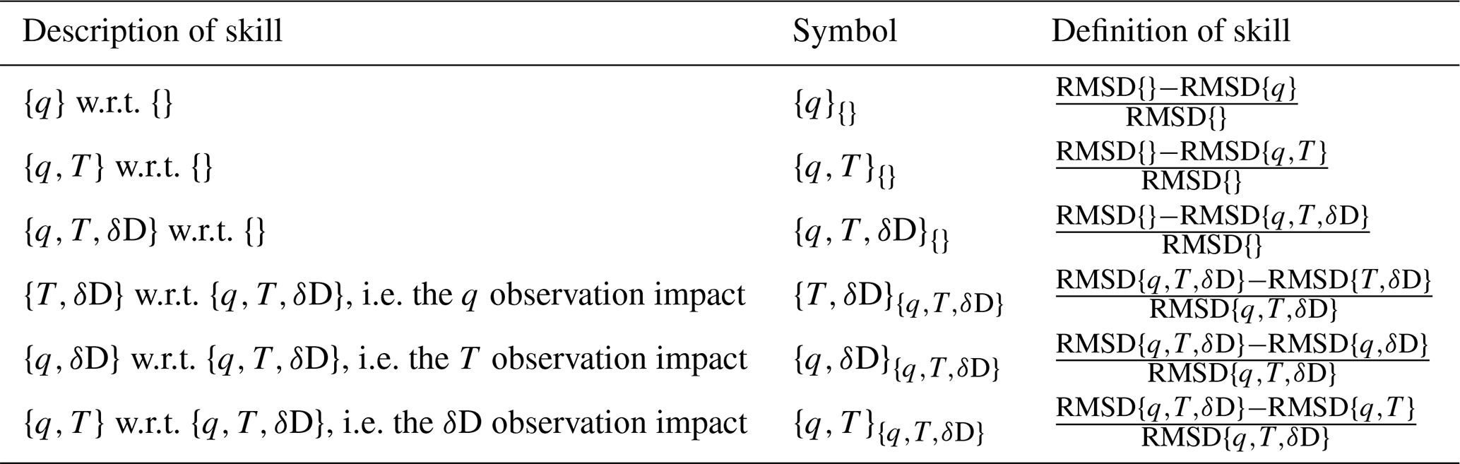
We calculate two different types of skill values. For the first type, we use the no-data assimilation as the reference assimilation experiment. Here positive values document the relative improvement of the analyses when assimilating observations with respect to using no observations (a reduction of the RMSD value by the assimilation of the observations). The first three items in Table 3 correspond to the respective skill values used in this study. For the second type, we use the assimilation of all observations (q, T, and δD together) as the reference and estimate the degradation of the analyses' quality (an increase of the RMSD value or a “loss of skill”) by removing one type of observation. By doing so, we can quantitatively compare the impact of the different observation types on the analyses' quality. In the following we refer to this skill value as the observation impact, where a more negative value corresponds to a stronger observation impact. The respective skill values that are discussed in this study are listed as the three last items in Table 3.
Table 3Skill values discussed in this study. The column “Description of skill” outlines which assimilation experiments are used for calculating the skills (the evaluated experiment and the reference experiment, with respect to which the evaluation is performed), the column “Symbol” shows the symbol used in the text when referring to the respective skill, and the column “Definition of skill” describes how the skill is calculated according to Eq. (8).
The Q2 values are calculated according to the budget analysis (Yanai et al., 1973):
where L is the latent heat of net condensation, q is the specific humidity, v is the horizontal wind vector, ω is the vertical velocity, and p is the pressure. Please note that the so-calculated Q2 might be slightly different from the real latent heating rates because it misinterprets changes in specific humidity caused by sub-scale transport (like small-scale turbulent mixing or diffusion) as latent heat release/consumption.
We work with 6-hourly analyses' data (for the 30° S–30° N region) of July and August 2016. The ensemble simulations are made using 96 different initial conditions. The ensemble mean at the beginning of the simulation period represents climatology. The first 3 weeks of the simulation (beginning of July) is a spin-up period, when the analyses gradually approximate the nature data by assimilating enough observations. In order to avoid impacts of this spin-up period, respective data are excluded from the evaluation study, which is then done for the period of mid-July to the end of August (covering 40.75 d).
Figure 1 shows the cumulative distribution functions (CDFs) of the variables q, T, δD, ω, Q2, and Prcp, calculated for the evaluated period from the nature data for all time steps and locations (black, full data set) and from the nature data belonging to a location and time step for which we can assimilate observations (green, data subset representing cloud-free conditions only). Only for T and δD do the full data set and the cloud-free data subset show similar CDFs. Concerning q, ω, Q2, and Prcp, the respective CDFs are significantly different. For q, all percentiles in the cloud-free data subset are shifted towards drier values when compared to the full data set. For ω, Q2, and Prcp, all distributions up to 50th percentiles are comparable for the full data set and the data subset; however, for large percentiles, the two CDFs differ significantly. The most extreme values (very low ω, very high Q2 and Prcp) are not present in the cloud-free data subset. This shows that we do not assimilate observations that directly represent the atmosphere of the locations and time steps where these extreme events take place.
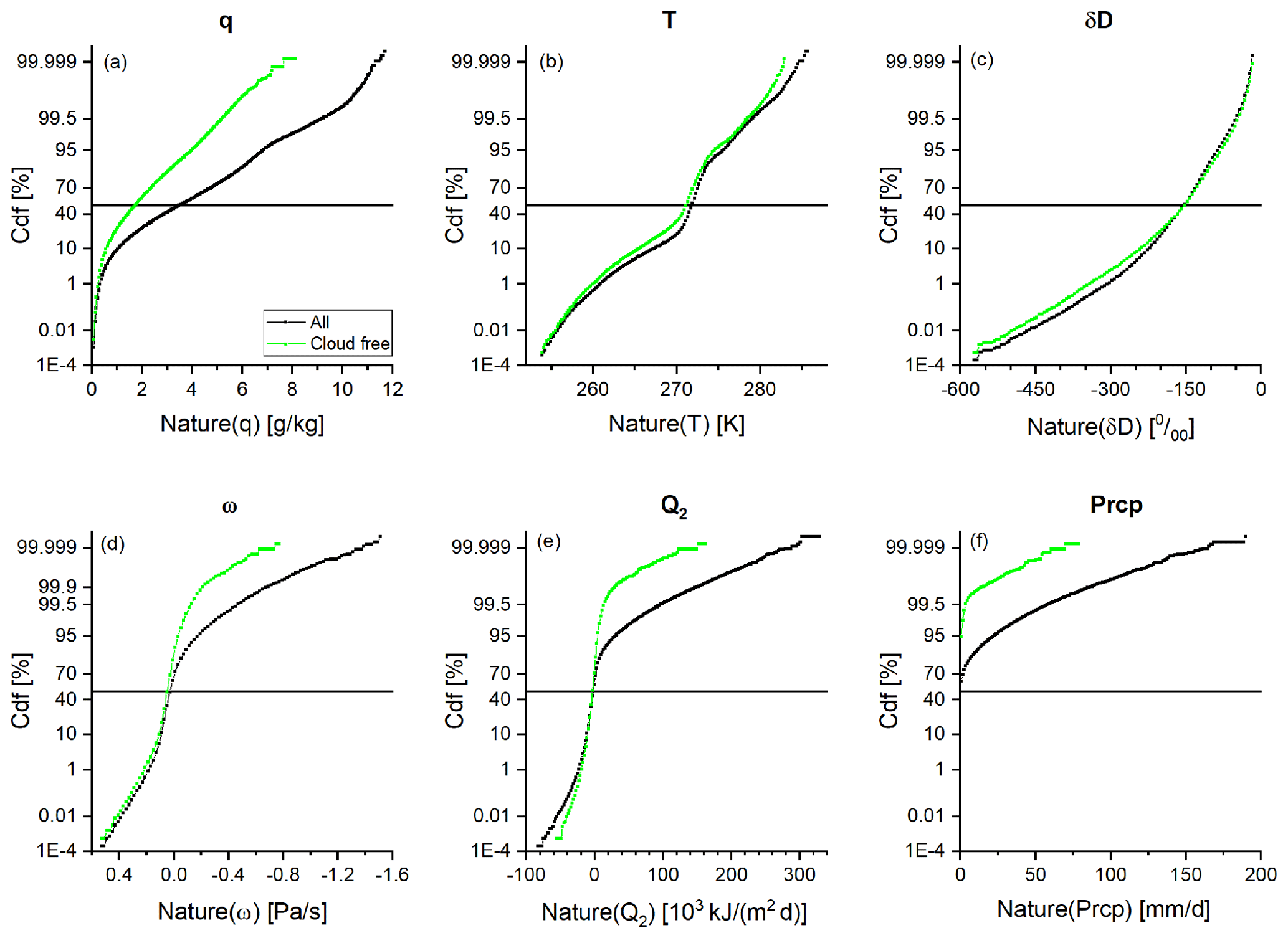
Figure 1Cumulative distribution functions (CDFs) of the analysed parameters as obtained from all nature data (black) and from the nature data belonging to cloud-free events (green). (a) For specific humidity (q), (b) for temperature (T), (c) for the isotopologue ratio (δD), (d) for vertical velocity (ω), (e) for latent heating (Q2), and (f) for precipitation (Prcp). The 50th percentile is indicated by the black line.
This section gives an overview on the assimilation impacts. For this purpose we calculate the RMSD values using all events (averaging is performed over all time steps and locations). Equation (7) can then be written as
where Nloc is the number of all locations (here we investigate the 30° S–30° N region with a 2.5° × 2.5° resolution, i.e. Nloc = 3600), and Ntim is the number of all time steps (here we work with 6 h time steps covering 40.75 d, i.e. Ntim = 163).
Because continuous time series are used for this calculation, we cannot assume independence of the different data when estimating the uncertainty of the RMSD values. For this reason, we use the circular block bootstrap method (e.g. Wilks, 2019) for the RMSD uncertainty estimation (the method is also explained in the Supplement of Toride et al., 2021). We resample these data 10 000 times, which provides a representative distribution of possible RMSD values. Here we use half of the difference between the respective 15.9th and 84.1th percentile estimates as the 1σ uncertainty of the RMSD value, which we then propagate to the skill values.
3.1 Skills with respect to the no-data assimilation
Observations of free-tropospheric q and T contain important information on the atmospheric state (among others on the water cycle variables ω, Q2, and Prcp) and are available as standard products from different satellite data processors at global scale, with daily coverage, and with good precision. Recently, respective observations of free-tropospheric δD have become available. We use the experiments that assimilate these observations in order to understand to what extent these observations help to constrain the model uncertainty.
First we calculate the skills achieved when assimilating q observations only using the no-data assimilation as the reference; i.e. here RMSDref of Eq. (8) is for ensemble means () obtained without assimilating any observation (no data are assimilated). This skill is referred to in the following as the {q}{} skill (see Table 3). The black lines in Fig. 2a–e show the vertical dependency of the {q}{} skills (for Prcp there is naturally no vertical dependency; Fig. 2f). The grey area around the lines indicates the 1σ uncertainty of the skills. Because we assimilate the observations of q at about 550 hPa, highest skill values are generally achieved in the free troposphere around 550 hPa. The dotted lines correspond to the pressure levels at 775 and 350 hPa, which delimits the vertical range we use as representative of the free troposphere and for which we perform dedicated evaluations in Sect. 4.
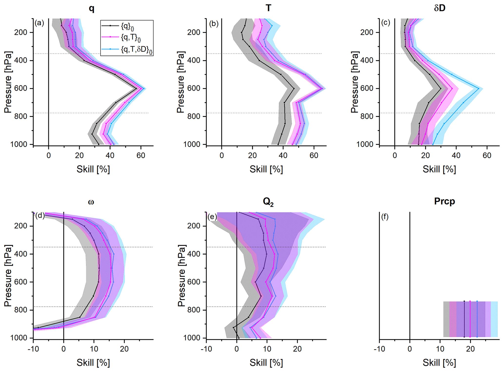
Figure 2Vertical profiles of the skills achieved by assimilating the observations (only q, q and T, and q, T, and δD) versus assimilating no observations. Black/grey: {q}{} skill. Magenta: {q,T}{} skill. Light blue: skill. The area around the lines represents the 1σ uncertainty. (a) For specific humidity (q), (b) for temperature (T), (c) for the isotopologue ratio (δD), (d) for vertical velocity (ω), (e) for latent heating (Q2), and (f) for precipitation (Prcp).
In a second experiment we assimilate observations of q together with T, which comes very close to an assimilation of relative humidity data. For the evaluation we again calculate the skills with respect to the no-data assimilation (in the following referred to as the {q,T}{} skill; see Table 3). The magenta lines in Fig. 2a–f give an overview on the achieved {q,T}{} skills. Compared to the {q}{} skills, these skills are larger in particular for T around 550 hPa (Fig. 2b) because T at 550 hPa is the additional observation we assimilate. The additional assimilation of T also has positive impacts on q and Q2 above 700 hPa and on δD between 500 and 300 hPa. By assimilating the standard observations q and T, we achieve skills of up to 60 % for q and T around 600 hPa. For the other variables (δD, ω, Q2, and Prcp) – for which no respective observations are assimilated – we also get skills that are often between 10 % and 30 %.
In a third experiment we test the impact when assimilating q, T, and δD observations together. For the evaluation we again calculate the skills with respect to the no-data assimilation (in the following referred to as the skill, respectively; see Table 3). The bright-blue lines in Fig. 2a–f give an overview on the achieved skills. The values are further improved when compared to the {q,T}{} skills: significantly for the δD (Fig. 2c; the respective δD skill is above 50 % at 600 hPa) but only slightly for the other variables. By significant, we mean that the skill values are larger than the estimated 1σ uncertainty of the skills, which is represented by the shaded area around the lines.
3.2 Observation impacts of q, T, and δD
Figure 2 reveals that assimilating q, T and δD observations at about 550 hPa constrains the uncertainty of free-tropospheric q, T, and δD simulations well between about 775 and 350 hPa (skill values up to 60 %). There is also a significant improvement for the simulated water cycle variables ω, Q2, and Prcp (skill values above 20 %). In this subsection, we examine the importance of the different types of observation (q, T, and δD, respectively) for achieving this quality for the analyses.
For this purpose we use the experiment that assimilates q, T, and δD observations together as the reference; i.e. RMSDref of Eq. (8) is for ensemble means () obtained when assimilating observations of q, T, and δD together. Then we compare this reference to an experiment for which one observation type has been removed and calculate the respective loss-of-skill values (see last three items of Table 3). A large negative loss-of-skill value means that the respective observation is very important for achieving the analyses' quality of the reference experiment; i.e. the respective observation has a strong impact on the analyses' quality. Our particular interest is in comparing the impact of δD observations that have only recently become available on a global scale and with daily coverage to the respective impacts of the traditionally used observations of q and T.
Figure 3a–f show these observation impacts. We first evaluate the impact of the q observations, which we determine by calculating the loss of skill when only assimilating observations of T and δD instead of assimilating all three observation types (i.e. the q observation impact is quantified by the skill value; see Table 3). The q observation impacts are represented by the dark-yellow line (and the shaded area is the respective 1σ uncertainty). We observe that, when removing q observations, we lose a lot of skill for all atmospheric variables; i.e. the q observations are important and have a strong impact on all the analysed variables. For the analyses of q the impact is strongest at 500–600 hPa (loss of skill of up to −50 %); for other vertical pressure levels the impact is smaller with loss-of-skill values above or close to −20 % (Fig. 3a). There is also a significant impact of q observations on the analyses of T, δD, Q2, ω, and Prcp (although less than for q): the skills are close to −20 % above 700 hPa for T (Fig. 3b), close to −15 % around 600 hPa for δD (Fig. 3c), and close to −10 % for free-tropospheric ω and Q2 (Fig. 3d and e) as well as for Prcp (Fig. 3f). By significant, we mean that the calculated loss-of-skill value is smaller than the estimated 1σ uncertainty of the skill, which is represented by the shaded area around the red line.
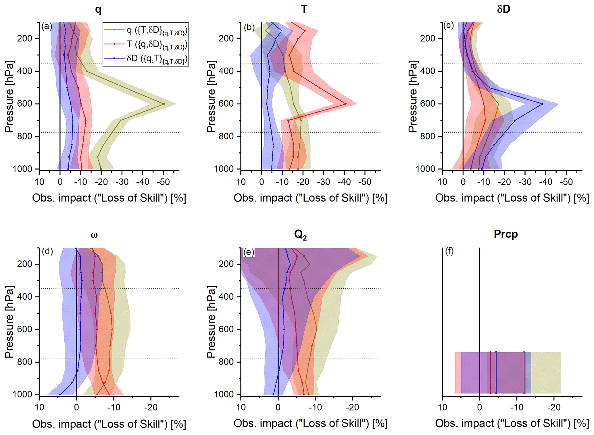
Figure 3Vertical profiles of observation impacts (loss of skill by removing one observation type from the reference experiment that considers all three observation types). Dark yellow: impact of q, represented by the skill. Red: impact of T, represented by the skill. Blue: impact of δD, represented by the skill. Panels (a)–(f) represent the different atmospheric variables as in Fig. 2.
The red line in Fig. 3 represents the T observation impact, which we quantify by the loss of skill when only assimilating observations of q and δD instead of assimilating all three observation types (the skill value; see Table 3). The T observation impact is highest for T. At 500–600 hPa, the respective loss-of-skill values are about −40 % and for other vertical pressure levels they are close to −15 % (Fig. 3b). The T observations also have a significant impact on the analyses of q, δD, Q2, ω, and Prcp (although less than for T): the skill values are close to −10 % above 600 hPa for q (Fig. 3a) and close to −10 % at 500–700 hPa for δD (Fig. 3c). For free-tropospheric ω and Q2, as well as for Prcp, the values are still about −5 % (Fig. 3d–f). However, for Prcp, this impact is not significant.
In a final setup, we investigate the loss of skills when only assimilating observations of q and T instead of all three observation types; i.e. we calculate the skill as a measure of the δD observation impact (see Table 3). The overview for the δD observation impact is shown as blue lines in Fig. 3. The strongest impact is observed for the δD analyses, with respective loss-of-skill values of close to −40 % around 600 hPa and about −10 % to −30 % for other pressure levels above 400 hPa (Fig. 3c), which is reasonable because observations of δD are important for achieving a high quality of the δD analyses. Concerning the q and T analyses, the δD observations have a significant impact above 500 hPa (for 900–500 hPa, the loss-of-skill values are about −5 %). For lower pressure levels, the δD observation impact on the q and T analyses is not significant (the loss-of-skill value is smaller than the estimated uncertainty; Fig. 3a and b). For ω and Q2, the δD observation impact is small and not significant ( skills of about −2.5 % only; Figs. 3d and e). For Prcp, we observe a loss-of-skill value of −5 %, which suggests that the δD observation impact on the Prcp analyses is slightly stronger than the respective T observation impact; however, it is not significant (compare red and blue lines in Fig. 3f).
The overview study of the previous section reveals that the δD observation impact is overall weak and generally much smaller than the respective impacts of the q and T observations. Theoretically the δD data contain unique information on phase transitions; i.e. it might be expected that δD observations can, in particular, improve the quality of the analyses for atmospheric conditions that involve strong and/or repeated cycles of condensation (or evaporation) processes. In this section, we examine the adequacy of this hypothesis in more detail and focus on the analyses of data averaged over a free-tropospheric pressure range (775–350 hPa, indicated by the dotted lines in Figs. 2 and 3).
4.1 Analyses' quality and vertical velocity
For vertically unstable atmospheric conditions, repeated cycles of condensation and evaporation take place. For this reason we can examine the aforementioned hypothesis by investigating the dependency of the δD observation impact on atmospheric vertical stability, and we use the mass-weighted average between 775 and 350 hPa of vertical velocity (free-tropospheric ω) as a proxy for atmospheric vertical stability.
Figure 4 depicts the dependency of the free-tropospheric analyses errors (the Δi,j values; see Eq. 6) on the free-tropospheric ω as simulated by the nature run (ωnat). As in Figs. 2 and 3, we investigate the analyses of the atmospheric variables q, T, δD, ω, Q2, and Prcp. We examine the low latitudes (30° S–30° N, with a 2.5° × 2.5° horizontal resolution) for 40 d with a 6-hourly time resolution; i.e. in total we have 586 800 events. In order to visualize the distribution of this large number of data points, we calculate the data densities as follows: we generate 60 equidistant ω bins covering all occurring ω values. Then we calculate the density distribution of the Δi,j values in each ω bin and sum the number of data points belonging to the highest Δi,j densities until we consider 98 % of all the Δi,j values occurring for a particular ω bin. These 98 % areas are depicted in Fig. 4. The grey shading represents the Δ{} distribution (i.e. for the Δi,j values when no observations are assimilated) and the magenta and blue lines the 98 % contour lines for the Δ{q,T} and distributions (i.e. for the Δi,j values achieved when we assimilate q and T observations and q, T, and δD observations, respectively).
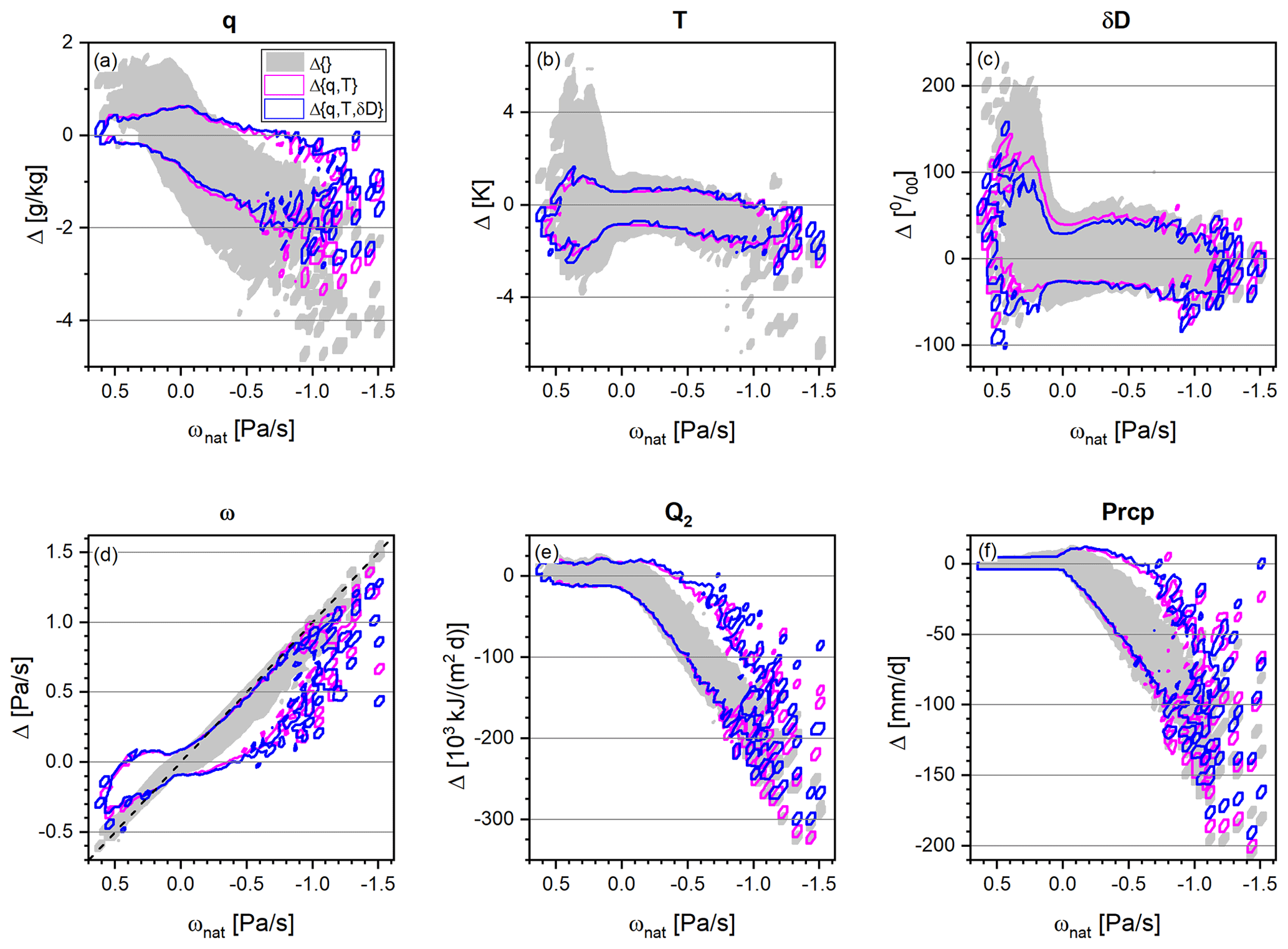
Figure 4Dependency of the free-tropospheric analyses errors (mass-weighted averages between 775 and 350 hPa) on the free-tropospheric vertical velocity (ωnat). Shown are the areas that contain 98 % of all the Δi,j values for a given ωnat value. Grey: 98 % area for the no-data assimilation (the Δ{}i,j data distribution). Magenta line: 98 % contour line for the data distribution. Blue line: 98 % contour line for the data distribution. (a) For specific humidity (q), (b) for temperature (T), (c) for the isotopologue ratio (δD), (d) for vertical velocity (ω), (e) for latent heating (Q2), and (f) for precipitation (Prcp).
Figure 4a–c show the distributions of the Δi,j values for the variables q, T, and δD. There is a weak correlation between the analyses errors and the ωnat data; i.e. the Δi,j values for q tend to be positive for stable atmospheric conditions (positive ω) and negative for unstable atmospheric conditions (strongly negative ω). A weak dependency is also observed in the Δi,j for T and to an even smaller extent in the Δi,j values for δD: in both cases the largest positive values occur for stable conditions (positive ω), and negative values are more frequent for unstable conditions (negative ω). The assimilation of q and T observations approximates the Δi,j values to the respective Δ-zero lines. Concerning the q analyses, the additional assimilation of δD observations further reduces the error in particular for strongly unstable conditions (for highly negative ωnat, the blue contour line better approximates the Δ-zero line than the magenta contour line; Fig. 4a). For T, the additional impact when assimilating δD observation is also slightly larger for unstable conditions (Fig. 4b). For δD , the additional impact of assimilating δD observations is most pronounced for stable conditions (blue contour lines better approximate the Δ-zero line than the magenta contour for positive ω values; Fig. 4c).
When no observations are assimilated, the strength of atmospheric stability can hardly be identified, and the ω error has the same magnitude as the actual ω value (the Δ{} distribution in Fig. 4d aligns very closely with the dashed black diagonal). The Δ{q,T} and distributions dissipate from the diagonal and approximate the Δ-zero line more well. This reduction of the ω error is slightly more pronounced for the than for the Δ{q,T} distributions and largest for the most negative actual ω values. However, despite the significant correction, the error is still largest for the most negative ω values. This means that, although the events of vertically unstable atmospheric conditions can be much better identified by assimilating the observations, the absolute strength of the instability is still underestimated.
For the analyses of latent heating (Q2; Fig. 4e) and precipitation rate (Prcp; Fig. 4f), the results are very similar to those of ω: without assimilating any data (Δ{} densities), the analyses are very uncertain for high heating rates (distribution of Δi,j values is far away from the respective Δ-zero lines). Actually, vertical velocity, precipitation rate, and heating rate are strongly correlated, which means that the events with strong latent heating and/or with high precipitation rates are almost not identified. By assimilating q and T observations, these errors can be strongly reduced. A further significant reduction (in particular for events when the error is very high) can be achieved by assimilating δD observations in addition to the observations of q and T.
4.2 The unique δD assimilation impact
Figure 4 suggests that when assimilating q and T together with δD, we get smaller analyses' errors for unstable atmospheric conditions than when only assimilating q and T. In this subsection, we quantify how the observation impacts depend on the atmospheric vertical stability.
Figure 5 shows the abundances of events corresponding to 13 different free-tropospheric vertical velocity (ω) bins. We have the highest abundances for ω values that are close to zero. The three bins corresponding to ωnat values between −0.09 and +0.06 Pa s−1 comprise together 441 253 out of 586 800 events, which is 75.20 %. Extreme vertical instabilities are rare; e.g. the bins corresponding to ωnat values smaller than −0.38 Pa s−1 only comprise 5363 events, i.e. 0.91 %. However, these extreme events are responsible for almost all the intense precipitation events, and it is very important to improve the analyses in a way that allows a better identification of these extreme events.
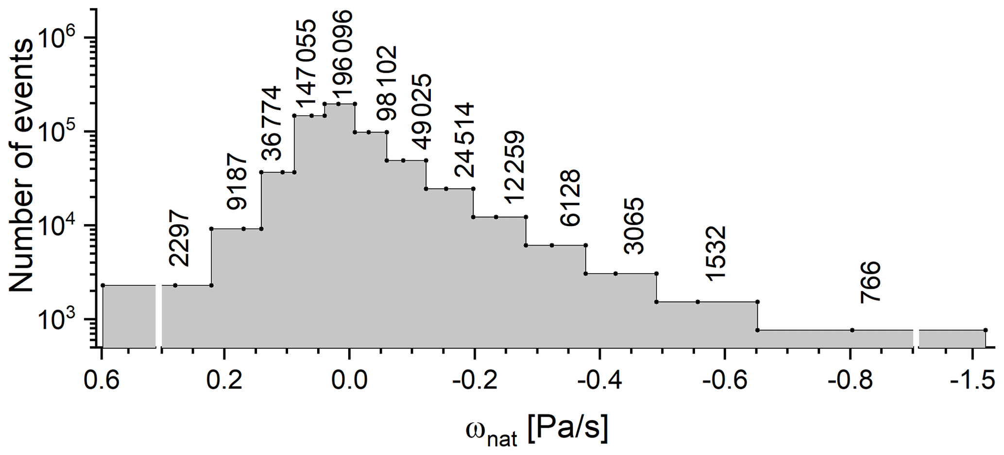
Figure 5Abundance chart showing the number of events for each of the 13 ω bins used for classifying atmospheric vertical stability conditions.
We use the binning from Fig. 5 for evaluating the dependence of the observation impacts on ω. As in Sect. 3, we quantify the observation impacts by the loss-of-skill values according to the last three items in Table 3. We calculate the respective RMSD values according to Eq. (7) for 13 different groups of events, A. Each group comprises the events showing free-tropospheric ω values as defined by the 13 different bins of Fig. 5. Because the events with strongly negative ω values (convective events) are generally individual events occurring on a single day, the respective groups of events do not consist of continuous time series. For the error estimation, we thus assume that the events of a certain ω group are independent (in the circular block bootstrap method, the block size is reduced to only one event).
Figure 6 depicts the observation impacts obtained for the 13 ωnat bins. The colours are as in Fig. 3. The q observation impact (quantified by the skill value, represented by the dark-yellow lines) is strong for all analysed variables (as already shown in Fig. 3). The highest q observation impact is found for q analyses at stable atmospheric conditions (loss-of-skill value of about −60 % for ωnat > +0.1 Pa s−1, Fig. 6a). For the T and δD analyses, the q observation impact is strongest, and for the analyses of ω, Q2, and Prcp, it is weakest for ωnat close to zero (Fig. 6b, c, and d–f, respectively). In summary, there is no clear systematic dependency of the q observation impact on atmospheric vertical stability.
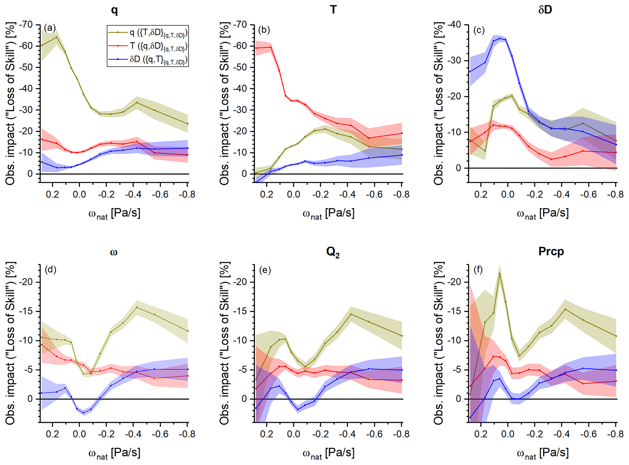
Figure 6Dependency of the free-tropospheric observation impacts (mass-weighted averages between 775 and 350 hPa) on the free-tropospheric vertical velocity (ωnat). The colours (dark yellow, red, and blue) and panels (a)–(f) are as in Fig. 3: they represent the different observation impacts and different analysed atmospheric variables, respectively.
The red lines represent the T observation impact (quantified by the skill value). It is strongest for the T analyses at stable atmospheric conditions (loss-of-skill value of about −60 % for ωnat > +0.1 Pa s−1; Fig. 6b). Concerning the analyses of the other atmospheric variables, the T observation impact shows generally a weak decrease with decreasing ωnat; i.e. the impact tends to be slightly stronger for stable than unstable atmospheric conditions (Fig. 6a, c–f).
The skill values quantify the δD observation impact, and they are depicted as blue lines in Fig. 6. The strongest δD observation impact is found for the δD analyses for stable atmospheric conditions (for ωnat > −0.05 Pa s−1, the respective loss-of-skill value is beyond −25 %; Fig. 6c). For the analyses of all other variables, the δD observation impact tends to be stronger for unstable conditions when compared to stable atmospheric conditions (Fig. 6a, b, d–f), thus showing the opposite behaviour to the T observation impact. While for moderately stable atmospheric conditions (ωnat > −0.2 Pa s−1), the T observation impact is significantly stronger than the δD observation impact, for unstable conditions (ωnat < −0.4 Pa s−1), the δD observation impact becomes as strong as the T observation impact or even slightly exceeds it. Because the large majority of events correspond to relatively stable atmospheric conditions (ωnat > −0.2 Pa s−1), the overview study as shown in Fig. 3 reveals an overall weak δD observation impact. However, for the infrequently occurring events corresponding to unstable atmospheric conditions, δD observations become at least as important as T observations for all variables except for T itself. This is particularly important for the analyses of ω, Q2, and Prcp because the most extreme ω, Q2, and Prcp values are relatively poorly identified by only assimilating q and T observations; a better identification of these events is achieved by the additional assimilation of δD (compare the magenta and blue contour lines in Fig. 4d–f).
Moreover, the relatively strong δD observation impact occurs for conditions when there are no observations assimilated: a thermal infrared sensor like IASI offers no free-tropospheric products for mid- or high-level clouds, which are typically present for ωnat < −0.4 Pa s−1 (see Fig. 1d). This suggests that the distinct free-tropospheric δD signals caused by atmospheric convection (e.g. Risi et al., 2008; Diekmann et al., 2021c) are well conserved in the δD fields modelled for cloud-free locations outside of the convective area. At cloud-free locations, the observations can then be exploited by the assimilation system, allowing for improvement of the analyses of the convective area. The δD observations seem to have a unique remote impact on the analyses of convective regions.
4.3 Simulations versus real-world data
In order to link our OSSE study to the real world, we examine similarities and differences of the {q,δD}-pair distributions between the simulated data used in this study and actual MUSICA IASI observational data. The {q,δD}-pair distributions can give valuable insight into the dominating atmospheric processes (mixing, shallow cloud formation, rainout, and convection and extreme precipitation events, Noone, 2012). Figure 7 shows these distributions for different data (sub)sets. Shown are the areas where the {q,δD} pairs have the highest densities and sum to 90 % (thick contour lines) and 50 % (thin contour lines) of all the data.
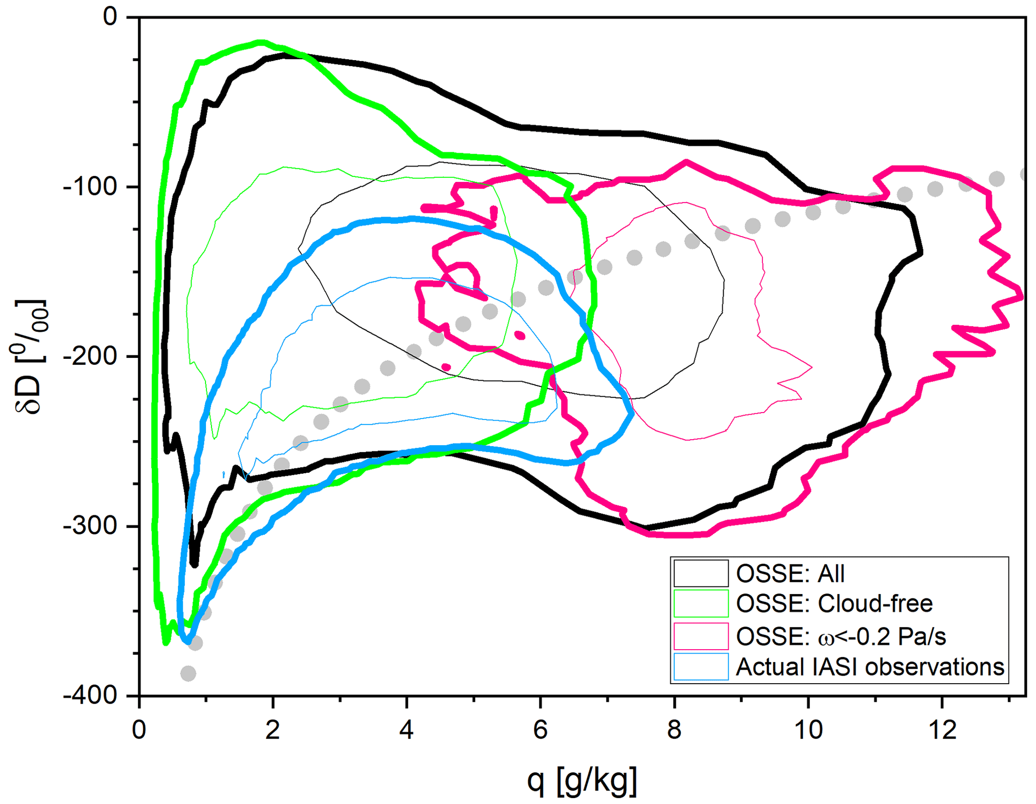
Figure 7Distributions of {q,δD} pairs at about 600 hPa as derived from the different data sets. Shown are the contour lines for the highest {q,δD}-pair data density (thick and thin lines show the areas containing 90 % and 50 % of all the data, respectively). Black line: all data from the nature run. Green line: cloud-free data from the nature run, i.e. data used as observations during the assimilation step. Pink line: nature run data corresponding to unstable atmospheric conditions (ωnat < −0.2 Pa s−1). Bright-blue line: actual IASI observation data. The dotted grey line is a typical tropical Rayleigh line, assuming the following atmospheric conditions over the ocean source location: T = 25 °C, RH = 80 %, and δD = −80‰.
Concerning the OSSE data, the black lines show the distribution for the full nature run data set (586 800 events for the studied 40 d and the 30° S–30° N area). The thick grey dotted line represents a typical tropical Rayleigh line (starting conditions: T = 25 °C, RH = 80 %, and δD = −80‰). A Rayleigh line describes the {q,δD} relation assuming that all the condensed water is immediately removed (immediate rainout). We observe that the {q,δD} pairs are well distributed around the Rayleigh line. For dry conditions, the data points tend to lie above the Rayleigh line, which indicates that the respective humidity levels are largely controlled by mixing between humid/enriched and dry/depleted water masses (Noone et al., 2011; González et al., 2016). For humid conditions, the data points tend to be situated below the Rayleigh line, i.e. in the super-Rayleigh domain (Noone, 2012). This strong depletion together with high humidity is caused by recurring evaporation and condensation; i.e. the same water mass experiences several condensation/evaporation processes in the atmosphere. This is a typical free-tropospheric {q,δD}-pair signal for convective activity (e.g. Risi et al., 2008; Blossey et al., 2010; Noone, 2012; Diekmann et al., 2021c, 2024).
The green contour lines represent the distribution for the atmospheric conditions, for which observations are assimilated in our assimilation studies. These are the cloud-free and stable atmospheric conditions. For this data subset, the {q,δD} pairs are mostly located below q = 6 g kg−1 and above the Rayleigh line, caused by the aforementioned dry air mass mixing.
The pink contour line comprises the events corresponding to unstable atmospheric conditions (ωnat < −0.2 Pa s−1). The respective {q,δD} pairs are generally located in the aforementioned super-Rayleigh domain, which suggests convective activity. From Figs. 4 and 6 we can conclude that the δD observations have the strongest impact on the analyses of the events with ωnat < −0.2 Pa s−1, i.e. for events where the {q,δD} pairs show this super-Rayleigh distribution. However, this is very different from the distribution of the assimilated data (green contour lines), revealing again that we do not assimilate observation of convective atmospheres (recall the discussion in the context of Fig. 1).
The {q,δD}-pair distribution obtained from actual MUSICA IASI observations is represented by the bright-blue contour lines in Fig. 7 for the same period and locations as the OSSE data. These real-world data are only available for a cloud-free atmosphere. Obviously, there is a significant difference between the {q,δD}-pair distribution simulated for cloud-free conditions and the actually observed distributions (compare green and bright-blue contour lines in Fig. 7). Whereas the q values in the simulations and the real-world observations are very similar, the respective δD values are systematically lower in the observations by about 50 ‰–100‰ when compared to the simulations (which is significantly larger than the systematic uncertainty estimated for the MUSICA IASI data after their calibration to in situ aircraft profiles; (Schneider et al., 2016). While in the simulations the large majority of the {q,δD} pairs is located above the Rayleigh line, in the observations about half is above, and the other half is below the Rayleigh line; i.e. a super-Rayleigh distribution is regularly observed in the real world but very rarely in the simulations. MUSICA IASI {q,δD}-pair data observed in the context of the West African monsoon are generally located below the Rayleigh line if a convective event was happening shortly before the observation (Sect. 6.3 of Diekmann, 2021; Diekmann et al., 2024), which highlights the strong link between the regularly observed super-Rayleigh distributions and convective processes. This link seems to be weaker in the simulations; i.e. there, the convective processes leave a significantly weaker {q,δD}-pair signature on the nearby cloud-free atmosphere.
4.4 Outlook on assimilating real-world δD observations
Current state-of-the-art satellite sensors allow the observation of δD with high quality and resolution (e.g. Worden et al., 2007; Frankenberg et al., 2009; Schneider and Hase, 2011; Lacour et al., 2012; Boesch et al., 2013; Worden et al., 2019; Schneider et al., 2020; Diekmann et al., 2021b). Furthermore, {q,δD}-pair super-Rayleigh distributions have been observed in data sets generated from measurements of the TES (Tropospheric Emission Spectrometer) satellite instrument (e.g. Noone, 2012) and in the MUSICA IASI data (Schneider et al., 2017; Diekmann et al., 2021b; Diekmann, 2021). As discussed in the previous subsection, these super-Rayleigh distributions contain valuable information on convective processes. In this context, the IASI instrument and thus the MUSICA IASI data set are promising in particular: measurements of IASI (or IASI-NG, the successor instrument of IASI) offer a very high horizontal and spatial coverage and are guaranteed at least for the next 2 decades in the framework of the Metop and Metop-SG missions of EUMETSAT (European Organisation for the Exploitation of Meteorological Satellites; https://www.eumetsat.int/our-satellites/metop-series, last access: 2 September 2024); i.e. respective {q,δD}-pair observations are guaranteed for the next decades.
However, in order to optimally use these δD observations in data assimilation approaches, we need isotopologue-enabled atmospheric models that capture as many details of a convective atmosphere as possible. The IsoGSM model used here with 200 × 200 km horizontal resolution generally does a good job, which has been demonstrated in different model validation studies (e.g. Yoshimura et al., 2008; Schneider et al., 2010). However, Fig. 7 reveals that IsoGSM systematically underestimates the impact of convective events on the {q,δD}-pair distribution of a cloud-free troposphere, which in turn suggests that in our OSSE study we might underestimate the real remote impact of δD observations on convective events. For achieving the optimal benefit from the real-world δD observations via a data assimilation approach, improving the modelled linkage between convective processes and the free-tropospheric {q,δD}-pair distribution might be an important next step. In this context, the ongoing development of including water isotopologue simulations into different high-resolution models also used for operational weather forecasting (e.g. Pfahl et al., 2012; Eckstein et al., 2018; Tanoue et al., 2023) is very encouraging. A higher horizontal resolution and a convection-permitting model setup (instead of parametrizing convection as in IsoGSM) might further improve the capability of a model for correctly capturing the real-world multi-scale impact of convective events (e.g. Pante and Knippertz, 2019) and thus better capture many details of convective processes (including the simulation of super-Rayleigh distributions).
In detail, we evaluate the quality of the analyses of low-latitudinal free-tropospheric specific humidity (q), temperature (T), and water vapour isotopologue ratio (δD), as well as of the three water cycle variables free-tropospheric vertical velocity (ω), free-tropospheric latent heating rate (Q2), and precipitation rate (Prcp). We investigate the impact of assimilating free-tropospheric specific humidity and temperature (which can be easily observed by many different techniques) and the possibility of further improving the analyses by additionally assimilating free-tropospheric water isotopologue data (δD), for which reliable observations with good horizontal and temporal coverage also exist nowadays. We assume that the observations are only available for cloud-free conditions.
First, we make a statistical overall evaluation considering all locations and time steps. The assimilation of q and T observations strongly improves the analyses' data quality of q and T with skill values of up to 60 % when compared to the no-data assimilation. Concerning the analyses of the other variables (δD, ω, Q2, and Prcp) we also achieve a strong improvement with skill values of 10 %–30 %. Assimilating δD on top of q and T strongly improves the analyses of δD even further (leading to a skill value of up to 50 %). However, the further improvement of the other variables (q, T, ω, Q2, and Prcp) is weak, and we found that the overall impact of δD observations on the analyses' quality is much smaller than the large impact caused by the observations of q and T.
In a second evaluation, we investigate how the δD observation impact depends on the atmospheric conditions. We use the atmospheric vertical velocity (ω) as a proxy for atmospheric stability. The large majority of events represent stable conditions, for which the δD observation impact is generally negligible; however, for the rare convective conditions with strongly negative ω, the δD observation impact is significant and for the analyses of the water cycle variables (ω, Q2, and Prcp) even slightly stronger than the T observation impact. Although being rare, the very unstable conditions dominate the total yearly averaged precipitation amounts in many regions, and they are also related to extreme events (e.g. storms, flooding) that are not well captured in the analyses (for these extreme events, the analyses errors of ω, Q2, and Prcp are also very large). This means that the δD observations offer potential for better capturing the events with the largest societal impact. Since unstable atmospheric conditions are almost always associated with clouds, we assimilate no observations at the location and time of these conditions. This hints at a unique remote impact of δD observations that are available elsewhere on the analyses of convective events.
A super-Rayleigh {q,δD}-pair distribution means high humidity and at the same time strong HDO depletion, and this distribution is linked to convective processes. We think that the conservation of these signals of isotopic depletion outside of the convecting area (where it can be measured) is essential for the unique remote impact of δD observations on the analyses of convective processes. In this context, we interpret the regular observation of super-Rayleigh distributions in the MUSICA IASI data as a promising indication that δD can have the same remote impact in the real world that it has in our OSSE study for the simulated world. A real-world δD assimilation works best if the model used correctly captures the HDO depletion of convection. The availability of a growing number of high-resolution isotopologue-enabled atmospheric models importantly supports further progress in this field.
The nature data and the ensemble mean data of the different assimilation experiments used for this study are available at https://doi.org/10.35097/PJeqXmWlLYSGBkJJ (Schneider et al., 2024). The MUSICA IASI water vapour isotopologue data set is available at https://doi.org/10.35097/415 (Diekmann et al., 2021a).
KY developed the isotopologue assimilation framework. KT conducted all the data assimilation experiments. MS developed the ideas for evaluating the analyses' improvements, achievable by adding δD observations, and did the respective calculations, whereby he was supported by KT and FK. FH, BE, and CJD provided important contributions for the design of this study. All authors supported the generation of the final version of this paper.
At least one of the (co-)authors is a member of the editorial board of Atmospheric Measurement Techniques. The peer-review process was guided by an independent editor, and the authors also have no other competing interests to declare.
Publisher's note: Copernicus Publications remains neutral with regard to jurisdictional claims made in the text, published maps, institutional affiliations, or any other geographical representation in this paper. While Copernicus Publications makes every effort to include appropriate place names, the final responsibility lies with the authors.
This research has benefit from funds of the Deutsche Forschungsgemeinschaft (provided for the project TEDDY, ID 416767181).
Important part of this work was performed on the supercomputer HoreKa, funded by the Ministry of Science, Research and Arts Baden-Württemberg and by the German Federal Ministry of Education and Research.
We acknowledge the support by the Deutsche Forschungsgemeinschaft and the Open Access Publishing Fund of the Karlsruhe Institute of Technology.
This research has been supported by the Deutsche Forschungsgemeinschaft provided for the project TEDDY, ID 416767181.
The supercomputing facilities used have been funded by the Ministry of Science, Research and Arts Baden-Württemberg and by the German Federal Ministry of Education and Research.
The article processing charges for this open-access publication were covered by the Karlsruhe Institute of Technology (KIT).
This paper was edited by Christof Janssen and reviewed by two anonymous referees.
Bailey, A., Nusbaumer, J., and Noone, D.: Precipitation efficiency derived from isotope ratios in water vapor distinguishes dynamical and microphysical influences on subtropical atmospheric constituents, J. Geophys. Res.-Atmos., 120, 9119–9137, https://doi.org/10.1002/2015JD023403, 2015. a
Blossey, P. N., Kuang, Z., and Romps, D. M.: Isotopic composition of water in the tropical tropopause layer in cloud-resolving simulations of an idealized tropical circulation, J. Geophys. Res.-Atmos., 115, D24309, https://doi.org/10.1029/2010JD014554, 2010. a, b
Boesch, H., Deutscher, N. M., Warneke, T., Byckling, K., Cogan, A. J., Griffith, D. W. T., Notholt, J., Parker, R. J., and Wang, Z.: HDOH2O ratio retrievals from GOSAT, Atmos. Meas. Tech., 6, 599–612, https://doi.org/10.5194/amt-6-599-2013, 2013. a, b
Bony, S., Risi, C., and Vimeux, F.: Influence of convective processes on the isotopic composition (δ18O and δD) of precipitation and water vapor in the tropics: 1. Radiative-convective equilibrium and Tropical Ocean–Global Atmosphere–Coupled Ocean-Atmosphere Response Experiment (TOGA-COARE) simulations, J. Geophys. Res.-Atmos., 113, D19305, https://doi.org/10.1029/2008JD009942, 2008. a
Bony, S., Stevens, B., Frierson, D., Jakob, C., Kageyama, M., Pincus, R., Shepherd, T. G., Sherwood, S. C., Siebesma, A. P., Sobel, A. H., Watanabe, M., and Webb, M. J.: Clouds, circulation and climate sensitivity, Nat. Geosci., 8, 261–268, https://doi.org/10.1038/ngeo2398, 2015. a
Chan, S. C. and Nigam, S.: Residual Diagnosis of Diabatic Heating from ERA-40 and NCEP Reanalyses: Intercomparisons with TRMM, J. Climate, 22, 414–428, https://doi.org/10.1175/2008JCLI2417.1, 2009. a
Clerbaux, C., Boynard, A., Clarisse, L., George, M., Hadji-Lazaro, J., Herbin, H., Hurtmans, D., Pommier, M., Razavi, A., Turquety, S., Wespes, C., and Coheur, P.-F.: Monitoring of atmospheric composition using the thermal infrared IASI/MetOp sounder, Atmos. Chem. Phys., 9, 6041–6054, https://doi.org/10.5194/acp-9-6041-2009, 2009. a
Dahinden, F., Aemisegger, F., Wernli, H., Schneider, M., Diekmann, C. J., Ertl, B., Knippertz, P., Werner, M., and Pfahl, S.: Disentangling different moisture transport pathways over the eastern subtropical North Atlantic using multi-platform isotope observations and high-resolution numerical modelling, Atmos. Chem. Phys., 21, 16319–16347, https://doi.org/10.5194/acp-21-16319-2021, 2021. a
Diekmann, C. J.: Analysis of stable water isotopes in tropospheric moisture during the West African Monsoon, PhD thesis, Karlsruher Institut für Technologie (KIT), https://doi.org/10.5445/IR/1000134744, 2021. a, b
Diekmann, C. J., Schneider, M., and Ertl, B.: MUSICA IASI water isotopologue pair product (a posteriori processing version 2), Institute of Meteorology and Climate Research, Atmospheric Trace Gases and Remote Sensing (IMK-ASF), Karlsruhe Institute of Technology (KIT) [data set], https://doi.org/10.35097/415, 2021a. a
Diekmann, C. J., Schneider, M., Ertl, B., Hase, F., García, O., Khosrawi, F., Sepúlveda, E., Knippertz, P., and Braesicke, P.: The global and multi-annual MUSICA IASI {H2O,δD} pair dataset, Earth Syst. Sci. Data, 13, 5273–5292, https://doi.org/10.5194/essd-13-5273-2021, 2021b. a, b, c, d, e, f
Diekmann, C. J., Schneider, M., Knippertz, P., de Vries, A. J., Pfahl, S., Aemisegger, F., Dahinden, F., Ertl, B., Khosrawi, F., Wernli, H., and Braesicke, P.: A Lagrangian Perspective on Stable Water Isotopes During the West African Monsoon, J. Geophys. Res.-Atmos., 126, e2021JD034895, https://doi.org/10.1029/2021JD034895, 2021c. a, b, c, d
Diekmann, C. J., Schneider, M., Knippertz, P., Trent, T., Boesch, H., Roehling, A. N., Worden, J., Ertl, B., Khosrawi, F., and Hase, F.: Water vapour isotopes over West Africa as observed from space: which processes control tropospheric H2O/HDO pair distributions?, EGUsphere [preprint], https://doi.org/10.5194/egusphere-2024-1613, 2024. a, b
Eckstein, J., Ruhnke, R., Pfahl, S., Christner, E., Diekmann, C., Dyroff, C., Reinert, D., Rieger, D., Schneider, M., Schröter, J., Zahn, A., and Braesicke, P.: From climatological to small-scale applications: simulating water isotopologues with ICON-ART-Iso (version 2.3), Geosci. Model Dev., 11, 5113–5133, https://doi.org/10.5194/gmd-11-5113-2018, 2018. a, b
Evans, C., Wood, K. M., Aberson, S. D., Archambault, H. M., Milrad, S. M., Bosart, L. F., Corbosiero, K. L., Davis, C. A., Pinto, J. R. D., Doyle, J., Fogarty, C., Galarneau, T. J., Grams, C. M., Griffin, K. S., Gyakum, J., Hart, R. E., Kitabatake, N., Lentink, H. S., McTaggart-Cowan, R., Perrie, W., Quinting, J. F. D., Reynolds, C. A., Riemer, M., Ritchie, E. A., Sun, Y., and Zhang, F.: The Extratropical Transition of Tropical Cyclones. Part I: Cyclone Evolution and Direct Impacts, Mon. Weather Rev., 145, 4317–4344, https://doi.org/10.1175/MWR-D-17-0027.1, 2017. a
Eyre, J. R., Bell, W., Cotton, J., English, S. J., Forsythe, M., Healy, S. B., and Pavelin, E. G.: Assimilation of satellite data in numerical weather prediction. Part II: Recent years, Q. J. Roy. Meteor. Soc., 148, 521–556, https://doi.org/10.1002/qj.4228, 2022. a
Field, R. D., Jones, D. B. A., and Brown, D. P.: Effects of postcondensation exchange on the isotopic composition of water in the atmosphere, J. Geophys. Res., 115, D24305, https://doi.org/10.1029/2010JD014334, 2010. a
Field, R. D., Kim, D., LeGrande, A. N., Worden, J., Kelley, M., and Schmidt, G. A.: Evaluating climate model performance in the tropics with retrievals of water isotopic composition from Aura TES, Geophys. Res. Lett., 41, 6030–6036, https://doi.org/10.1002/2014GL060572, 2014GL060572, 2014. a, b
Fink, A. H., Pohle, S., Pinto, J. G., and Knippertz, P.: Diagnosing the influence of diabatic processes on the explosive deepening of extratropical cyclones, Geophys. Res. Lett., 39, L07803, https://doi.org/10.1029/2012GL051025, l07803, 2012. a
Frankenberg, C., Yoshimura, K., Warneke, T., Aben, I., Butz, A., Deutscher, N., Griffith, D., Hase, F., Notholt, J., Schneider, M., Schrejver, H., and Röckmann, T.: Dynamic processes governing lower-tropospheric HDOH2O ratios as observed from space and ground, Science, 325, 1374–1377, https://doi.org/10.1126/science.1173791, 2009. a, b
Galewsky, J., Steen-Larsen, H. C., Field, R. D., Worden, J., Risi, C., and Schneider, M.: Stable isotopes in atmospheric water vapor and applications to the hydrologic cycle, Rev. Geophys., 54, 809–865, https://doi.org/10.1002/2015RG000512, 2016. a
González, Y., Schneider, M., Dyroff, C., Rodríguez, S., Christner, E., García, O. E., Cuevas, E., Bustos, J. J., Ramos, R., Guirado-Fuentes, C., Barthlott, S., Wiegele, A., and Sepúlveda, E.: Detecting moisture transport pathways to the subtropical North Atlantic free troposphere using paired H2O-δD in situ measurements, Atmos. Chem. Phys., 16, 4251–4269, https://doi.org/10.5194/acp-16-4251-2016, 2016. a, b, c, d
Hersbach, H., Bell, B., Berrisford, P., Hirahara, S., Horányi, A., Muñoz Sabater, J., Nicolas, J., Peubey, C., Radu, R., Schepers, D., Simmons, A., Soci, C., Abdalla, S., Abellan, X., Balsamo, G., Bechtold, P., Biavati, G., Bidlot, J., Bonavita, M., De Chiara, G., Dahlgren, P., Dee, D., Diamantakis, M., Dragani, R., Flemming, J., Forbes, R., Fuentes, M., Geer, A., Haimberger, L., Healy, S., Hogan, R. J., Hólm, E., Janisková, M., Keeley, S., Laloyaux, P., Lopez, P., Lupu, C., Radnoti, G., de Rosnay, P., Rozum, I., Vamborg, F., Villaume, S., and Thépaut, J.-N.: The ERA5 global reanalysis, Q. J. Roy. Meteorol. Soc., 146, 1999–2049, https://doi.org/10.1002/qj.3803, 2020. a
Hunt, B. R., Kostelich, E. J., and Szunyogh, I.: Efficient data assimilation for spatiotemporal chaos: A local ensemble transform Kalman filter, Physica D, 230, 112–126, https://doi.org/10.1016/j.physd.2006.11.008, 2007. a
Kalman, R. E.: A New Approach to Linear Filtering and Prediction Problems, J. Basic Eng.-T. ASME, 82, 35–45, https://doi.org/10.1115/1.3662552, 1960. a
Lacour, J.-L., Risi, C., Clarisse, L., Bony, S., Hurtmans, D., Clerbaux, C., and Coheur, P.-F.: Mid-tropospheric δD observations from IASI/MetOp at high spatial and temporal resolution, Atmos. Chem. Phys., 12, 10817–10832, https://doi.org/10.5194/acp-12-10817-2012, 2012. a, b
Lacour, J.-L., Flamant, C., Risi, C., Clerbaux, C., and Coheur, P.-F.: Importance of the Saharan heat low in controlling the North Atlantic free tropospheric humidity budget deduced from IASI δD observations, Atmos. Chem. Phys., 17, 9645–9663, https://doi.org/10.5194/acp-17-9645-2017, 2017. a
Ling, J. and Zhang, C.: Diabatic Heating Profiles in Recent Global Reanalyses, J. Climate, 26, 3307–3325, https://doi.org/10.1175/JCLI-D-12-00384.1, 2013. a
Noone, D.: Pairing Measurements of the Water Vapor Isotope Ratio with Humidity to Deduce Atmospheric Moistening and Dehydration in the Tropical Midtroposphere, J. Climate, 25, 4476–4494, https://doi.org/10.1175/JCLI-D-11-00582.1, 2012. a, b, c, d, e, f
Noone, D., Galewsky, J., Sharp, Z. D., Worden, J., Barnes, J., Baer, D., Bailey, A., Brown, D. P., Christensen, L., Crosson, E., Dong, F., Hurley, J. V., Johnson, L. R., Strong, M., Toohey, D., Van Pelt, A., and Wright, J. S.: Properties of air mass mixing and humidity in the subtropics from measurements of the D/H isotope ratio of water vapor at the Mauna Loa Observatory, J. Geophys. Res.-Atmos., 116, D22113, https://doi.org/10.1029/2011JD015773, 2011. a, b, c
Pante, G. and Knippertz, P.: Resolving Sahelian thunderstorms improves mid-latitude weather forecasts, Nat. Commun., 10, 3487, https://doi.org/10.1038/s41467-019-11081-4, 2019. a
Pfahl, S., Wernli, H., and Yoshimura, K.: The isotopic composition of precipitation from a winter storm – a case study with the limited-area model COSMOiso, Atmos. Chem. Phys., 12, 1629–1648, https://doi.org/10.5194/acp-12-1629-2012, 2012. a, b
Risi, C., Bony, S., and Vimeux, F.: Influence of convective processes on the isotopic composition (δ18O and δD) of precipitation and water vapor in the tropics: 2. Physical interpretation of the amount effect, J. Geophys. Res.-Atmos., 113, D19306, https://doi.org/10.1029/2008JD009943, 2008. a, b, c
Risi, C., Bony, S., Vimeux, F., and Jouzel, J.: Water-stable isotopes in the LMDZ4 general circulation model: Model evaluation for present-day and past climates and applications to climatic interpretations of tropical isotopic records, J. Geophys. Res.-Atmos., 115, D12118, https://doi.org/10.1029/2009JD013255, 2010. a
Risi, C., Noone, D., Worden, J., Frankenberg, C., Stiller, G., Kiefer, M., Funke, B., Walker, K., Bernath, P., Schneider, M., Bony, S., Lee, J., Brown, D., and Sturm, C.: Process-evaluation of tropospheric humidity simulated by general circulation models using water vapor isotopic observations. Part 2: Using isotopic diagnostic to understand the mid and upper tropospheric moist bias in the tropics and subtropics, J. Geophys. Res., 117, D05304, https://doi.org/10.1029/2011JD016623, 2012. a
Rodgers, C.: Inverse Methods for Atmospheric Sounding: Theory and Praxis, World Scientific Publishing Co., Singapore, ISBN 981-02-2740-X, 2000. a
Schneider, A., Borsdorff, T., aan de Brugh, J., Aemisegger, F., Feist, D. G., Kivi, R., Hase, F., Schneider, M., and Landgraf, J.: First data set of columns from the Tropospheric Monitoring Instrument (TROPOMI), Atmos. Meas. Tech., 13, 85–100, https://doi.org/10.5194/amt-13-85-2020, 2020. a, b
Schneider, M. and Hase, F.: Optimal estimation of tropospheric H2O and δD with IASI/METOP, Atmos. Chem. Phys., 11, 11207–11220, https://doi.org/10.5194/acp-11-11207-2011, 2011. a, b
Schneider, M., Yoshimura, K., Hase, F., and Blumenstock, T.: The ground-based FTIR network's potential for investigating the atmospheric water cycle, Atmos. Chem. Phys., 10, 3427–3442, https://doi.org/10.5194/acp-10-3427-2010, 2010. a
Schneider, M., Wiegele, A., Barthlott, S., González, Y., Christner, E., Dyroff, C., García, O. E., Hase, F., Blumenstock, T., Sepúlveda, E., Mengistu Tsidu, G., Takele Kenea, S., Rodríguez, S., and Andrey, J.: Accomplishments of the MUSICA project to provide accurate, long-term, global and high-resolution observations of tropospheric {H2O,δD} pairs – a review, Atmos. Meas. Tech., 9, 2845–2875, https://doi.org/10.5194/amt-9-2845-2016, 2016. a, b
Schneider, M., Borger, C., Wiegele, A., Hase, F., García, O. E., Sepúlveda, E., and Werner, M.: MUSICA MetOp/IASI {H2O,δD} pair retrieval simulations for validating tropospheric moisture pathways in atmospheric models, Atmos. Meas. Tech., 10, 507–525, https://doi.org/10.5194/amt-10-507-2017, 2017. a, b
Schneider, M., Ertl, B., Diekmann, C. J., Khosrawi, F., Weber, A., Hase, F., Höpfner, M., García, O. E., Sepúlveda, E., and Kinnison, D.: Design and description of the MUSICA IASI full retrieval product, Earth Syst. Sci. Data, 14, 709–742, https://doi.org/10.5194/essd-14-709-2022, 2022. a
Schneider, M., Toride, K., and Yoshimura, K.: MUSICA IASI water isotopologue OSSE assimilation experiments (used in AMT study), Institute of Meteorology and Climate Research, Atmospheric Trace Gases and Remote Sensing (IMKASF), Karlsruhe Institute of Technology (KIT) [data set], https://doi.org/10.35097/PJeqXmWlLYSGBkJJ, 2024. a
Sherwood, S. C., Bony, S., and Dufresne, J.-L.: Spread in model climate sensitivity traced to atmospheric convective mixing, Nature, 505, 37–42, https://doi.org/10.1038/nature12829, 2014. a
Tada, M., Yoshimura, K., and Toride, K.: Improving weather forecasting by assimilation of water vapor isotopes, Scientific Reports, 11, 18067, https://doi.org/10.1038/s41598-021-97476-0, 2021. a, b
Tanoue, M., Yashiro, H., Takano, Y., Yoshimura, K., Kodama, C., and Satoh, M.: Modeling Water Isotopes Using a Global Non-Hydrostatic Model With an Explicit Convection: Comparison With Gridded Data Sets and Site Observations, J. Geophys. Res.-Atmos., 128, e2021JD036419, https://doi.org/10.1029/2021JD036419, 2023. a, b
Toride, K., Yoshimura, K., Tada, M., Diekmann, C., Ertl, B., Khosrawi, F., and Schneider, M.: Potential of Mid-tropospheric Water Vapor Isotopes to Improve Large-Scale Circulation and Weather Predictability, Geophys. Res. Lett., 48, e2020GL091698, https://doi.org/10.1029/2020GL091698, 2021. a, b, c, d, e, f, g, h
Webster, C. R. and Heymsfield, A. J.: Water Isotope Ratios H/D, 18O16O, 17O16O in and out of Clouds Map Dehydration Pathways, Science, 302, 1742–1745, https://doi.org/10.1126/science.1089496, 2003. a
Werner, M., Langebroek, P. M., Carlsen, T., Herold, M., and Lohmann, G.: Stable water isotopes in the ECHAM5 general circulation model: Toward high-resolution isotope modeling on a global scale, J. Geophys. Res.-Atmos., 116, D15109, https://doi.org/10.1029/2011JD015681, 2011. a
Wilks, D. S.: Statistical methods in the atmospheric sciences, Elsevier, https://doi.org/10.1016/C2017-0-03921-6, 2019. a
Worden, J., Noone, D., Bowman, K., Beer, R., Eldering, A., Fisher, B., Gunson, M., Goldman, A., Herman, R., Kulawik, S. S., Lampel, M., Osterman, G., Rinsland, C., Rodgers, C., Sander, S., Shephard, M., Webster, R., and Worden, H.: Importance of rain evaporation and continental convection in the tropical water cycle, Nature, 445, 528–532, https://doi.org/10.1038/nature05508, 2007. a, b, c
Worden, J. R., Kulawik, S. S., Fu, D., Payne, V. H., Lipton, A. E., Polonsky, I., He, Y., Cady-Pereira, K., Moncet, J.-L., Herman, R. L., Irion, F. W., and Bowman, K. W.: Characterization and evaluation of AIRS-based estimates of the deuterium content of water vapor, Atmos. Meas. Tech., 12, 2331–2339, https://doi.org/10.5194/amt-12-2331-2019, 2019. a, b
Yanai, M., Esbensen, S., and Chu, J.-H.: Determination of Bulk Properties of Tropical Cloud Clusters from Large-Scale Heat and Moisture Budgets, J. Atmos. Sci., 30, 611–627, https://doi.org/10.1175/1520-0469(1973)030<0611:DOBPOT>2.0.CO;2, 1973. a
Yoshimura, K., Kanamitsu, M., Noone, D., and Oki, T.: Historical isotope simulation using Reanalysis atmospheric data, J. Geophys. Res., 113, D19108, https://doi.org/10.1029/2008JD010074, 2008. a, b, c
Yoshimura, K., Miyoshi, T., and Kanamitsu, M.: Observation system simulation experiments using water vapor isotope information, J. Geophys. Res.-Atmos., 119, 7842–7862, https://doi.org/10.1002/2014JD021662, 2014. a, b