the Creative Commons Attribution 4.0 License.
the Creative Commons Attribution 4.0 License.
 | 12 Sep 2024
The EarthCARE lidar cloud and aerosol profile processor (A-PRO): the A-AER, A-EBD, A-TC, and A-ICE products
David Patrick Donovan
Gerd-Jan van Zadelhoff
Ping Wang
ATLID (ATmospheric LIDar) is the lidar flown on the multi-instrument Earth Cloud Aerosol and Radiation Explorer (EarthCARE). EarthCARE is a joint ESA–JAXA mission that was launched in May 2024. ATLID is a three-channel, linearly polarized, high-spectral-resolution lidar (HSRL) system operating at 355 nm. Cloud and aerosol optical properties are key EarthCARE products. This paper provides an overview of the ATLID Level 2a (L2a; i.e., single instrument) retrieval algorithms being developed and implemented in order to derive cloud and aerosol optical properties. The L2a lidar algorithms that retrieve the aerosol and cloud optical property profiles and classify the detected targets are grouped together in the so-called A-PRO (ATLID-profile) processor. The A-PRO processor produces the ATLID L2a aerosol product (A-AER); the extinction, backscatter, and depolarization product (A-EBD); the ATLID L2a target classification product (A-TC); and the ATLID L2a ice microphysical estimation product (A-ICE). This paper provides an overview of the processor and its component algorithms.
- Article
(24215 KB) - Full-text XML
- BibTeX
- EndNote


The Earth Cloud Aerosol and Radiation Explorer mission (EarthCARE) (Illingworth et al., 2015) is a multi-instrument cloud–aerosol–radiation-process-study-oriented mission embarking a high-spectral-resolution atmospheric lidar (ATLID), a Doppler cloud profiling radar (CPR), a multi-spectral imager (MSI), and a three-view broadband radiometer (BBR). EarthCARE will measure the global-height-resolved distribution of clouds, aerosols, and precipitation and estimate their macrophysical, microphysical, and radiative properties (Wehr et al., 2023).
This document describes the algorithms within the EarthCARE L2a ATLID profile processor (A-PRO). Within the EarthCARE project, single-instrument geophysical property retrievals are referred to as L2a retrievals (Eisinger et al., 2024). A-PRO has been developed with support from the European Space Agency (ESA) for specific application to ATLID (do Carmo et al., 2021) and comprises a number of new developments. Within this processor, four main sub-algorithms exist: a procedure aimed at deriving the large-scale aerosol (and thin cloud) extinction and backscatter (A-AER), an optimal-estimation-based extinction and backscatter retrieval algorithm (A-EBD), a lidar target classification procedure (A-TC), and an ice microphysical property estimation procedure (A-ICE). Output products corresponding to each of these component procedures are generated. Collectively, these algorithms produce multiple-horizontal-resolution profiles of lidar extinction, backscatter, optical depth, particle type, ice effective radius, ice water content, and target type (e.g., cloud phase, aerosol type). This paper presents the theoretical background of the algorithms that comprise the A-PRO processor and presents and discusses various examples. The examples shown are based on the simulations described in Donovan et al. (2023).
ATLID
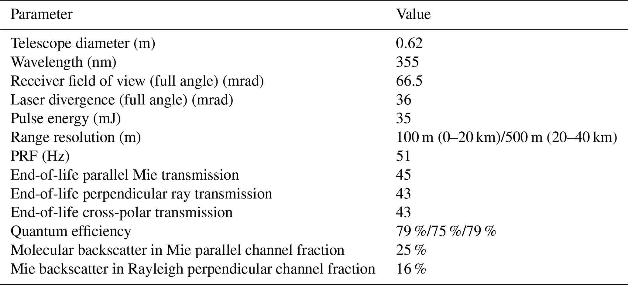
ATLID is a linearly polarized three-channel lidar operating at 355 nm. The vertical resolution of the return signal is about 100 m throughout most of the atmosphere. The pulse repetition frequency (PRF) is 51 Hz, and nominally it is planned that two shots will be averaged on board, giving a horizontal resolution on the order of 305 m. The lidar delivers profiles of the parallel particulate attenuated backscatter (ATB), the Rayleigh (molecular) attenuated backscatter, and the perpendicular particulate attenuated backscatter.
ATLID is a so-called high-spectral-resolution lidar (HSRL) (Eloranta, 2005). The first successfully operating HSRL system emphasizing aerosol and cloud sensing was flown in 2022 (Liu et al., 2024; Dai et al., 2024). The Aerosol and Carbon Detection Lidar (ACDL), on board the Atmospheric Environment Monitoring Satellite known as Daqi-1 (DQ-1), uses an atomic iodine filter technique at 532 nm (Dong et al., 2018) to separate molecular and particulate backscattering. A HSRL lidar that previously operated (2018–2023) at the same wavelength as ATLID was Aeolus (Straume et al., 2020). Aeolus, unlike ATLID, was primarily oriented to the retrieval of line-of-sight winds; however, aerosol and cloud algorithms were also developed and applied to Aeolus data (Flament et al., 2021; Ehlers et al., 2022). Aeolus cloud and aerosol products are limited by the characteristic of Aeolus (e.g., limited vertical resolution and the lack of a depolarization channel). Nevertheless, useful aerosol and cloud products can be retrieved. Indeed, some of the techniques originally developed for ATLID and described in this paper have been successfully “back-ported” to Aeolus (Wang et al., 2024). Unlike Aeolus, ATLID has been optimized exclusively for aerosol and cloud sensing. Thus, even more useful aerosol and cloud products are expected from ATLID.
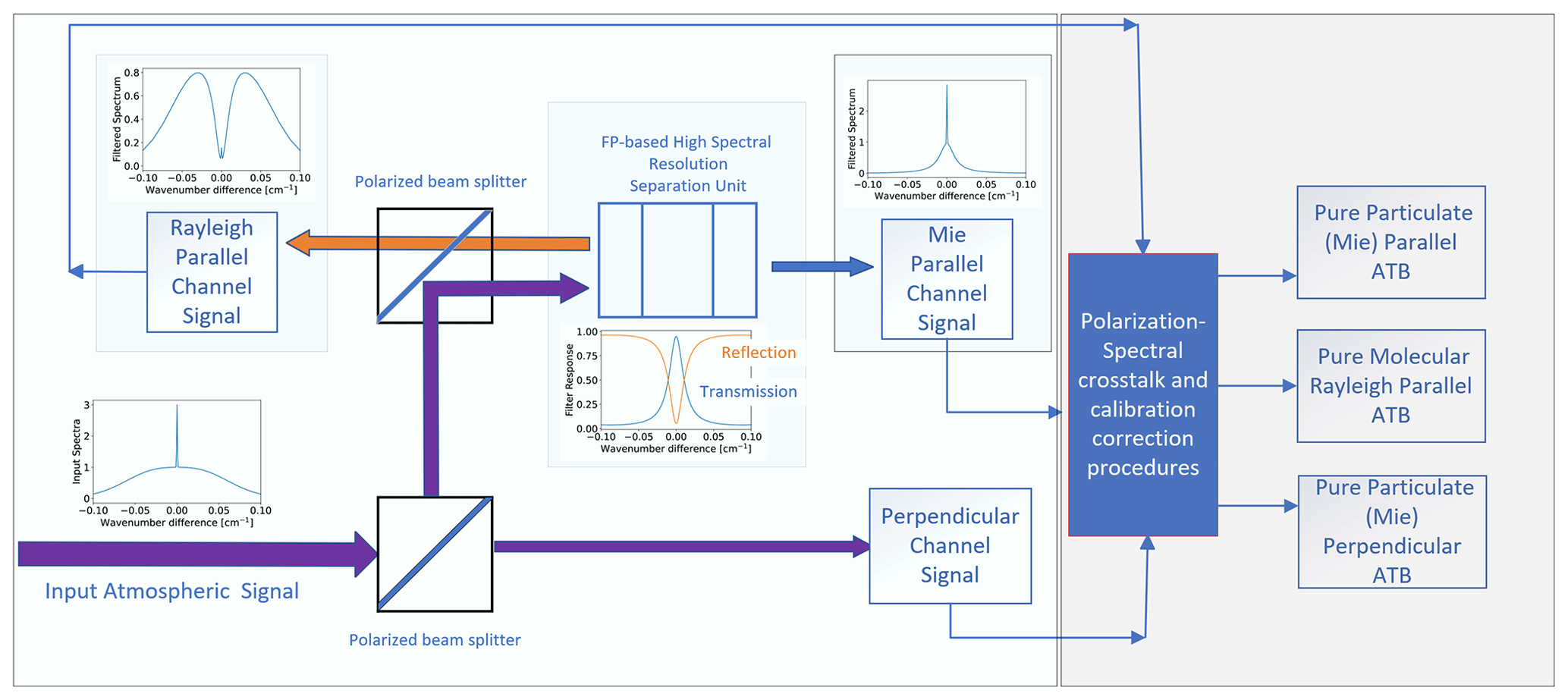
ATLID, uses a Fabry–Pérot etalon to (imperfectly) separate the spectrally narrow return from aerosols and clouds (“Mie”) from the thermally broadened return from atmospheric molecules (“Rayleigh”). Note that Mie scattering properly refers only to scattering by perfect spheres. In this paper (and indeed through much of EarthCARE-related documentation) the term is used rather loosely to broadly cover what should be termed “particulate” scattering. Further, the term Rayleigh scattering is also used loosely. A more accurate term would be “molecular” or “Rayleigh–Brillouin” scattering. Since the Rayleigh and Mie signal separation is imperfect, a degree of crosstalk between the channels exists. In order to separately quantify the pure Mie and Rayleigh scattering contributions, a crosstalk correction procedure is applied as part of the level-1 (L1) processing. ATLID emits linearly polarized light and separates the returned backscatter into components polarized parallel and perpendicular to the plane defined by the emitted beam. The polarization separation comes before the HSRL spectral filter. Accordingly, the three ATLID physical channels are as follows:
-
a parallel (or co-polar) Mie channel,
-
a parallel (or co-polar) Rayleigh channel,
-
a perpendicular (or cross-polar) channel.
For details of ATLID's design, see do Carmo et al. (2016) and do Carmo et al. (2021). Some of the important ATLID technical specifications are repeated in Table 1.
A simple depiction of the ATLID receiver operation and level-1 (L1) processing is presented in Fig. 1. Here the left section of the figure depicts the hardware components, while the right section depicts the application of the crosstalk correction and calibration procedures carried out by the L1 processing software. The perpendicular detection channel measures the depolarized signals from a combination of molecular Rayleigh and particulate scattering; however, the level-1 (L1) ATLID processor spectral-polarization crosstalk correction procedure applied to the detected signals delivers the perpendicular signals due to particulate scattering only. The crosstalk monitoring and correction procedures use a combination of averaged high-altitude (e.g., 30–40 km) pure molecular Rayleigh scattering returns, (non-water) surface returns, and suitable cloud returns to determine the relative amount of crosstalk present in each channel. Once the crosstalk coefficients are specified, absolute calibration is linked mainly to the use of high-altitude (e.g., 30–40 km) pure molecular Rayleigh scattering returns. Calibration and crosstalk correction issues are not described further here. It is anticipated that these specific topics, however, will be the subject of a detailed post-launch publication.
After spectral and polarization crosstalk correction and calibration, the ATLID attenuated backscatter coefficient profiles can be related to the atmospheric extinction and backscatter coefficients (neglecting multiple-scattering effects for the time being) as follows:
where bR is the Rayleigh attenuated backscatter, is the parallel Mie attenuated backscatter, is the perpendicular Mie attenuated backscatter, z is the atmospheric altitude, and r(z) is the range from the lidar. The corresponding p terms represent the detected power. αM is the aerosol and cloud extinction, and αR is the atmospheric Rayleigh extinction. is the parallel Mie backscatter, βR is the Rayleigh backscatter, and is the perpendicular Mie backscatter. Referring to Eqs. (2) and (3), the total Mie attenuated backscatter is given by
In general, for space-based lidars, multiple scattering can be an important contributor to the detected signals and must be accounted for (Winker, 2003). In this work, a novel approach has been used that lies in terms of speed and accuracy between the simple effective extinction approach due to Platt (1981) and the approach of Hogan (2008). The multiple-scattering formalism used in this work is detailed in Appendix B.
The primary function of the ATLID level-2 (L2) A-PRO processor is to invert the lidar signals to obtain estimates of backscatter and extinction and using these values together with the particle linear depolarization ratio () in order to classify the detected targets.
In principle, HSRL retrievals can yield direct estimates of extinction and backscatter profiles (Eloranta, 2005); however, the direct method for estimating the backscatter involves calculating the ratio of the Mie (Eq. 4) and Rayleigh (Eq. 1) signals, while the extinction estimation involves taking the range derivative of the logarithm of the Rayleigh signal (Eq. 1). Both of these mathematical operations are sensitive to noise, particularly when small (or even possibly negative) values may be present in the Rayleigh channel. Thus, direct inversions are only practical when the data are of a suitably high signal-to-noise ratio (SNR).
The SNR of the attenuated HSRL backscatter signals can be increased by along-track averaging of the signals. However, this can produce, at best, biased results and, at worst, ambiguous or non-physical results if, for example, “strong” (e.g., cloud) and “weak” signals are averaged indiscriminately together. Thus, any averaging of the signals must respect the structure of the atmospheric scene being probed. Aerosol fields may be homogeneous enough and the signals weak enough that averaging along track for several tens of kilometers may be justified. On the other hand, cloud returns may be strong and inhomogeneous to the point that it is desirable to apply inversions on the finest available resolution.
What is required is a means to guide the averaging of the signals when appropriate and a multi-scale approach for retrieving optical properties and target classification for both aerosols and clouds. The A-PRO processor structure is designed with such goals in mind.
2.1 General structure
A-PRO is divided into three main algorithms, as depicted in Fig. 2.
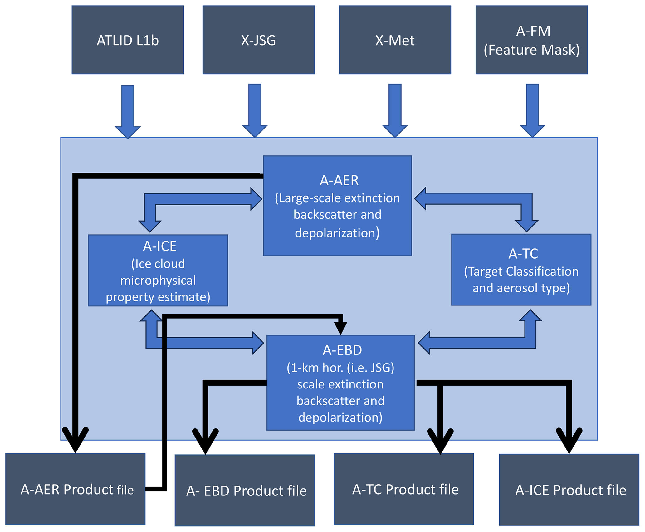
Figure 2Schematic depiction of the high-level structure of the A-PRO processor. The top dark grey boxes represent the input products, while the bottom dark grey boxes represent the output products. The double-headed arrows are used to indicate that the data flow is bidirectional between the main procedures (A-AER and A-EBD) and the A-ICE- and A-TC-related procedures.
The following list details the main inputs to A-PRO.
- L1 ATLID product
-
This provides calibrated crosstalk-corrected attenuated backscatter (ATB) profiles.
- X-JSG auxiliary data product
-
This is the Joint Standard Grid product, which facilitates the co-location of the EarthCARE L2 products with one another (Eisinger et al., 2022). The X-JSG essentially provides a common coordinate system for the EarthCARE instruments. In addition, the JSG contains explicit information used to map the indices of the ATLID L1 data to the common grid. This strategy was adopted in order to help insure consistent geolocation and to avoid the need for downstream processors (which may combine ATLID and/or CPR and/or MSI L1 or L2 products) to perform their own regridding. The X-JSG horizontal resolution is about 1 km, and the vertical resolution follows the ATLID vertical grid.
- X-MET auxiliary data product
-
X-MET contains the atmospheric pressure, temperature, etc., built using ECMWF forecast data (Eisinger et al., 2022).
- A-FM L2 product
-
The ATLID feature mask provides a high-resolution mask of detected targets. The use of A-FM helps facilitate the appropriate averaging of the data. A-FM uses a combination of image-processing techniques in order to identify regions of clouds and aerosols, surface returns, clear air, or attenuated regions. The detected aerosol and cloud regions are separated into cloud phase and aerosol type later in subsequent processing steps.
The A-FM product variable most relevant for A-PRO is the feature mask index with ranges between 0− and 10 (for non attenuated and non-surface pixels), which is based on the probability of a cloud or aerosol target being present in the particulate backscatter. Thus, the index is a reflection of the SNR of the Mie attenuated backscatter. Thus, higher indices are usually associated with, e.g., thick clouds, and lower indices are usually associated with, e.g., optically thinner aerosols. Attenuated regions are identified using the Rayleigh channel.
The feature mask index is produced using a combination of the iterative-application edge-preserving median-hybrid filters (Russ, 2007) of different dimensions (e.g., 11 horizontal pixels × 11 vertical pixels and 11 × 3 pixels), the removal of detected features, and the iterative application (with up to 200 iterations) of a Gaussian smoothing kernel (with a Gaussian width of, e.g., 13 × 1.5 pixels) together with a noise level estimation procedure. Features are detected and recorded for a fixed sequence of iterations (e.g., after 15, 70, 140, and 200 iterations). Thus, A-FM output are inherently “multi-scale”, but the approach is, in a sense, more continuous due to the iteration convolution approach, compared to, e.g., the fixed averaging interval strategy used by the CALIPSO vertical feature mask algorithm (Vaughan et al., 2009). Details of A-FM can be found in van Zadelhoff et al. (2023b).
Within A-PRO the following main procedures are present.
-
Aerosol-oriented extinction and backscatter retrieval (A-AER) This procedure uses direct HSRL retrieval methods for determining extinction and backscatter on large horizontal (e.g. 50 km+) scales (e.g., deriving the extinction based on the log derivative of the Rayleigh signal Eloranta, 2005). In order to do this the lidar signals must be appropriately masked and averaged to achieve a target SNR while avoiding mixing different data together (e.g., clouds and aerosol). The averaging mask originates, in part, from the A-FM output, which is used to avoid averaging strong and weak features together. The methods used by A-AER to estimate extinction and backscatter are described in Sect. 2.2 and Appendix A. A-AER outputs are directly used by the high-horizontal-resolution A-EBD component of A-PRO.
-
Cloud and aerosol extinction, backscatter, and depolarization procedure (A-EBD) This routine retrieves the aerosol and cloud extinction and backscatter profiles at the 1 km horizontal scale. At this scale, the SNR of the molecular scattering channel return is too low to enable the techniques employed by the A-AER approach. Instead, the method relies on a forward-modeling optimal estimation (OE) approach. As a priori information, the lidar ratio (S) estimates produced by A-AER are used as inputs in A-EBD. In order to deal with the generally low SNR of the lidar data at high horizontal resolutions and to improve the run time of the algorithm, A-EBD operates on a layer-by-layer basis. That is, for each aerosol or cloud layer (which may span a number of range gates), the lidar ratio is assumed to be constant. A-EBD is described in detail in Sect. 2.3.
-
Target classification procedure (A-TC) A-TC uses the extinction, backscatter, and depolarization ratio and auxiliary inputs such as ECMWF forecast temperature in order to classify targets into classes such as water or ice cloud or aerosol type. The aerosol typing scheme is based primarily on using the lidar ratio and particle depolarization ratio to assign the aerosol to a type (Wandinger et al., 2023). The cloud-phase determination scheme uses layer-integrated backscatter and depolarization in a manner similar to that employed for the CALIOP retrievals (Hu et al., 2009).
-
Ice microphysical property estimation (A-ICE) A-ICE employs a simple parameterization approach for estimating ice cloud effective radius and ice water content (IWC) using retrieved extinction values. In particular, an empirical parameterization based on in situ observations that uses temperature and extinction is employed (Heymsfield et al., 2014).
The above components work in a cooperative fashion. A-AER provides a first pass focusing on the optically thin targets, and A-EBD performs another pass to retrieve both the optically thick and thin targets using A-AER output as input. A-TC and A-ICE component procedures are used by both A-AER and A-EBD.
2.2 A-AER
The A-AER procedure retrieves the large-scale optical properties of the optically thin regions (weak features) and sets the stage for the high-resolution A-EBD stage of the A-PRO procedure. Thus, in addition to providing estimates of extinction and lidar ratio, A-AER also provides the column-by-column layer structure and a priori classification used as input by E-EBD. The inputs are the L1b ATLID data (attenuated crosstalk-corrected backscatters for the three ATLID channels), the ATLID feature mask (A-FM) product (van Zadelhoff et al., 2023b), the auxiliary X-JSG (joint standard grid multi-instrument grid definition), and the X-MET (ECMWF-supplied meteorological fields) product (Eisinger et al., 2022).
2.2.1 Pre-processing
Due to the generally low SNR of lidar signals at a horizontal scale of a few kilometers, before the A-AER procedure can derive quantitative extinction and lidar ratios and determine the layering structure and layer classification, averaging of the input L1 attenuated backscatters is necessary. This averaging, however, must respect the structure of the observations to avoid, e.g., averaging both cloud and aerosol regions together. Thus, a large part of what A-AER does involves pre-processing the attenuated backscatters based on the observed structure of the observations themselves before final quantitative values of extinction and lidar ratio are derived. This “pre-processing” is schematically described in Fig. 3, which corresponds to steps (1) to (7) in the more detailed overall A-AER algorithm flowchart shown in Fig. 4 described in Sect. 2.2.2.
Referring to Fig. 3, first the ATBs are binned according to the JSG definition in Fig. 3a. Then the A-FM data are also binned to the X-JSG as in Fig. 3b. The X-JSG-binned A-FM index is then used to separate strong and weak features by applying a threshold in order to create a mask as in Fig. 3c. The mask is then used to separately smooth the strong- and weak-featured ATBs using a box car window (typically 40 horizontal × 1 or 3 vertical pixels) (see also step 3 in Fig. 4). After smoothing, the strong and weak fields are merged to produce the “hybrid smoothed ATBs” (Fig. 3e), which have improved SNRs compared to the input signals but have not had their main features blurred out.
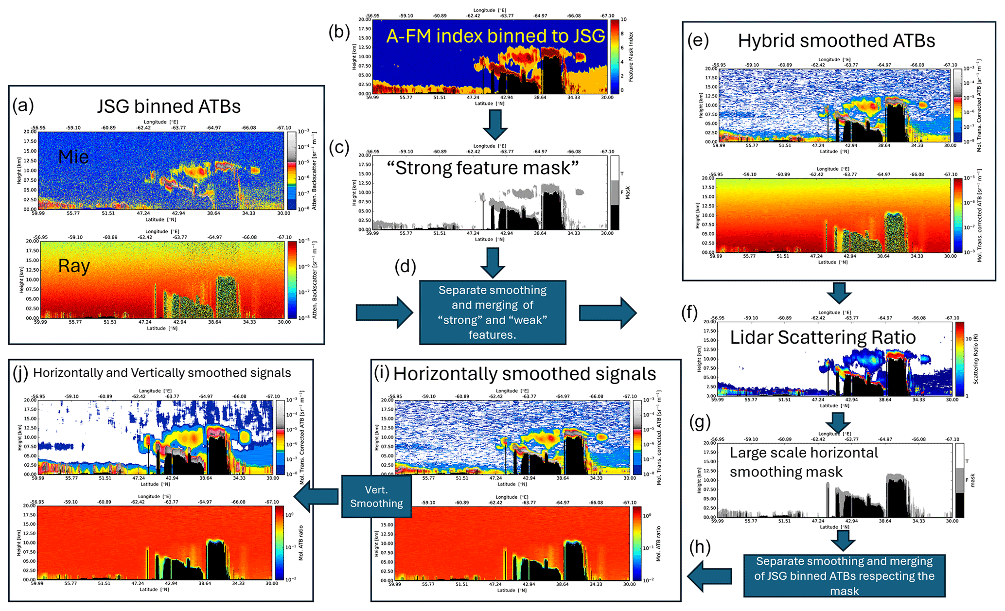
Figure 3Conceptual depiction of the A-AER pre-processing illustrated using simulated data corresponding to the Halifax scene (Donovan et al., 2023). The processing steps depicted here correspond to steps 1 to 7 in Fig. 4.
The Rayleigh and Mie hybrid smoothed ATBs generally have associated SNRs suitable for the useful calculation of backscatter and scattering ratios but not for the direct determination of extinction or lidar ratios. Thus, further guided smoothing is needed. The A-FM indices could be used directly as a guide; however, this was found to be problematic since low index values can be produced by attenuation rather than the absence of a significant target. Accordingly, the ray and Mie hybrid smoothed ATBs are then used to estimate the lidar scattering ratio (f):
By using R for further masking we will have, in a sense, accounted for attenuation in the smoothing mask definition procedure. To create the mask used in the next averaging steps, an atmospheric-density-dependent threshold is applied to the scattering ratio (Fig. 3g). The masked and unmasked data fields are then separately horizontally averaged (e.g., up to 50 km) and merged (Fig. 3h) and finally vertically averaged (e.g., by 1 to 4 km) (Fig. 3i). More detail on this process is given in the description associated with steps (5) and (6) of Fig. 4.
2.2.2 Full algorithm description
A flowchart depiction of the main elements of the A-AER procedure is presented in Fig. 4. The inputs are represented by the upper-right parallelograms.
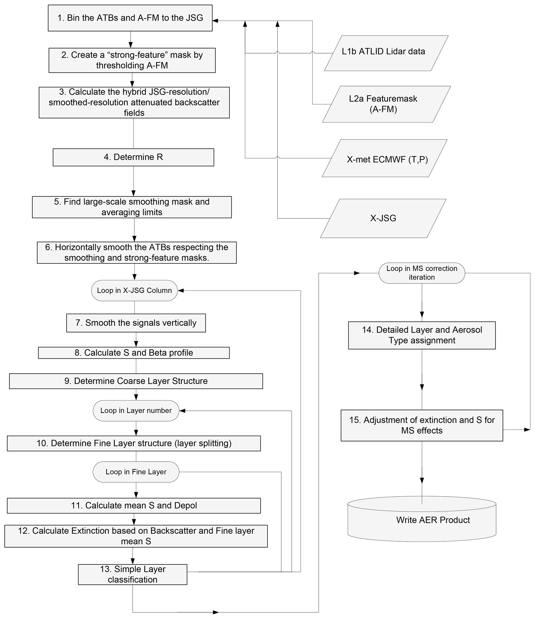
Figure 4Schematic depiction of the structure of the A-AER components of the A-PRO processor.
In step 1 the level-1 ATBs are rebinned according to the JSG grid. At the same time, the associated errors in the ATB profiles are generated either by calculating the standard deviation of the ATBs or by quadratically summing the error estimates coming from the ATLID L1 product. A-FM data that are at native ATLID resolution are also put onto the JSG. In the case of the A-FM data, the A-FM feature probability indices are not averaged. The highest index within the appropriate JSG pixel is used instead, except in the case where the input indices contain a surface detection indication; in those cases the JSG pixel is flagged as a surface pixel. In this step, the temperature, pressure, and atmospheric number density for each JSG pixel are also determined using the X-MET auxiliary product.
Step 2 is to create a mask to guide the horizontal averaging of the input ATBs. A strong feature mask is created by thresholding the JSG-gridded A-FM product. This mask is then used in step 3 to smooth the data in respect to the mask.
In step 3, the JSG-gridded ATBs are averaged using a moving-average box car, but pixels identified as either strong features or weak features are not segregated and are averaged separately. The smoothed strong-feature and weak-feature pixels are then merged together. The strong-feature A-FM threshold and the averaging window are both configurable. The prelaunch defaults are set to ≥ 8 (corresponding to likely cloud) for the A-FM index threshold and 1 vertical by 40 horizontal JSG pixels for the averaging window. The setting of these configuration parameters, along with any others, will be re-evaluated during commissioning phase (and indeed throughout the mission lifetime) using in-orbit observations.
In step 4 the lidar scattering ratio is calculated along with corresponding error estimates using the ATBs resulting from the previous step. These scattering ratio estimates are then used in the next step to create a mask to help guide the horizontal averaging that will be ultimately applied to the ATBs.
In step 5, the altitude-dependent limits that will be applied on a column-by-column basis in order to average the ATBs in preparation for the quantitative determination of extinction and backscatter are found. The first sub-step is to define a mask representing pixels where it is considered valid to average over horizontally. This mask is first built by masking out the following kinds of pixels:
-
fully attenuated pixels;
-
surface pixels;
-
pixels with an associated scattering ratio at 355 nm (as calculated in Step 4) above a specified threshold, e.g., corresponding to the scattering ratio at the surface (this threshold is reduced with height according to the atmospheric density profile, i.e., , where zs is the surface altitude and Rth is the threshold value, and setting Rth = 2 corresponds to a particulate backscatter threshold of about 1.6 × 10⁻⁵ [m−1 sr−1]).
Averaging attenuated regions (e.g., below optical thick clouds) together with unattenuated regions would ultimately lead to inaccurate extinction and backscatter profiles. In order to avoid this, the averaging mask is set to false for all altitudes in each respective column that are below the highest altitude of the mask in the given column. In addition, single-pixel isolated true mask values (i.e., a true value completely surrounded by false values) are set to false.
The height- and time-dependent horizontal averaging limits are then found. This is accomplished by first considering a box centered around the JSG column in question. Following this the height-averaged SNR of the resulting horizontally averaged Rayleigh ATB is calculated using all the data identified by the averaging mask. If this average SNR is below a set threshold (e.g., 50), the horizontal extent of the box is expanded until the threshold is met or a specific maximum box extent is reached. The average weak-feature ATBs for all three channels and their respective error estimates are then calculated (step 6) for each height bin.
In step 7, the weak-feature Mie ATBs are corrected for the effects of Rayleigh transmission and are smoothed vertically using a sliding linear least-square fitting procedure. The same is done for the ratio of the Rayleigh ATB to molecular backscatter. The fitting window is configurable (e.g., five vertical range bins). The use of a linear fit provides a natural way to handle the edge effects at the top altitudes and the near-ground pixels; i.e., linear extrapolation is used to find appropriate values of the pixels closer within a distance less than half the width of the fitting window from the top of the profile or the ground. The use of a sliding linear fit enables the range derivative of the signals to be calculated in the same step in a consistent manner. This procedure produces the following horizontally and vertically smoothed quantities:
where and
where the Rat superscript in Eq. (9) is used to indicate that the ratio between the observed molecular-extinction-corrected attenuated Rayleigh backscatter and the unattenuated Rayleigh backscatter is being used. In Eqs. (6)–(9), Fhv is used to denote the masked vertical and horizontal smoothing operation, and τRay is the Rayleigh optical depth from the top of the atmosphere to the height in question. For simplicity the range dependence is not written explicitly here.
Step 8 involves the estimation of the particulate lidar ratio S, the extinction, and the backscatter. The outputs of the previous step (i.e., Eqs. 6–8) are used. Depending on the configuration, this can be accomplished in two ways. Which method is applied can be selected as a configuration option. One of the methods is built using a conventional log-derivation approach for estimating the extinction profile, the other uses a new “local forward-modeling approach”. The two different approaches are described and discussed in Appendix A. The new approach generally produces better-behaved extinction-to-backscatter ratio profiles. This is important since in subsequent steps the A-EBD algorithm will separate and classify layers in part using the extinction-to-backscatter ratio. S is also a primary input to the A-EBD algorithm. No multiple-scattering correction is performed at this stage, since that can only be done once a target classification has been performed.
In step 9 the coarse-layer structure is calculated. The JSG gridded A-FM indices are used along with the scattering ratio calculations performed in the previous step. This process is described in detail in Irbah et al. (2023). In brief, layer boundaries are assigned whenever significant changes in the JSG A-FM indices or significant differences in temperature and/or scattering ratio are encountered. In addition, layers whose vertical extent is above a specified threshold (e.g. 2 km) are split into two.
In step 10 each coarse layer is examined to see if the layer should be further subdivided. The basic idea is to test if it is valid to represent the layer as a homogeneous entity or if it is better to split the layer into a number of homogeneous sub-layers. The procedure relies on examining the behavior of a reduced Chi-squared goodness-of-fit variable applied to the scattering ratio, lidar ratio, and depolarization ratio, which is calculated for all possible sub-layering for up to four distinct sub-layers. This process can be somewhat computationally demanding for extended regions, meaning that it is notably more efficient to employ a coarse layer and splitting process to find the fine-layer structure rather than trying to directly determine the fine-layer structure. The layer-splitting algorithm is described in more detail in Sect. 2.1.2 of Irbah et al. (2023).
An example of the determined layer boundaries using a subsection of the Halifax scene is shown in Fig. 5. The coarse-layer boundaries (shown in black) were determined using the FM index and scattering ratios. Within the cloud-free aerosol columns there is little contrast in the scattering ratio and the FM indices, respectively. The aerosol layer is divided into two coarse layers in any case, since its extent would otherwise exceed the maximum allowed extent (here set to 4 km). It can also be seen that the fine-layer determination procedure results in the coarse layers being further divided here, usually into three or four sub-layers.
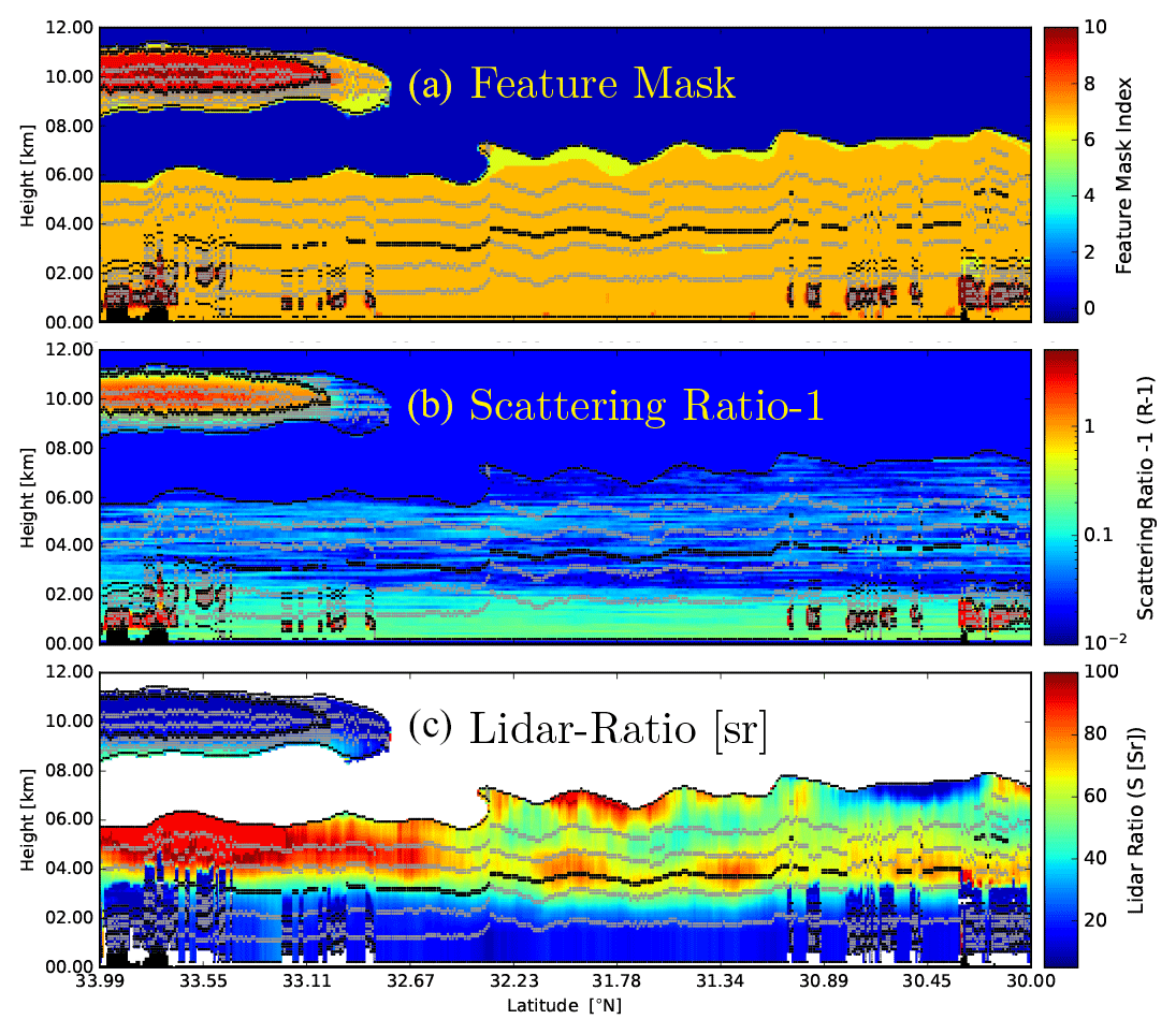
Figure 5Layer tops and bottoms over-plotted on the A-FM index, the scattering ratio −1 (as calculated in step 4), and the lidar ratio (as calculated in step 8). The black lines represent the coarse-layer boundaries, while the grey lines represent the fine-layer boundaries.
Based on the fine-layer structure calculated in step 10, the mean backscatter, extinction, lidar ratio, and depolarization ratio are calculated. This information is then passed to the classification procedures (steps 13 and 14), which are described in Sect. 2.2 and 2.3 of Irbah et al. (2023). The simple classification procedure (step 13) can be viewed as a backup that can be used when the detailed classification procedure (step 14) cannot be applied reliably and is used in the A-EBD component of A-PRO. It should be noted that extinction and backscatter information used at this stage have not been corrected for multiple-scattering effects; thus, the classification procedures are performed using a version of the classification priors adjusted to approximately account for MS effects (e.g., reduced effective lidar ratio in ice clouds).
In step 15 the extinction and lidar ratio values calculated in step 9 are corrected for multiple-scattering effects. The treatment of multiple scattering is treated in general within Appendix B, and the specific adjustment of the values for extinction and backscatter within A-AER are treated within Sect. B4. After the MS correction, to maintain consistency the layers are then re-classified using a call to the A-TC procedures, but this time the classification priors appropriate for single scattering are used.
After steps 1–15 are completed for the whole frame, the data product file is written out including the layering and classification information.
2.3 A-EBD
After A-AER has been executed, the ATLID extinction backscatter and depolarization procedure is applied. The core of this procedure is built upon a column-by-column optimal estimation (OE) forward-model inversion performed at a higher resolution than A-AER with the aim of supplying extinction and backscatter values for both weak and strong targets. A-EBD uses the classification and (where possible) the lidar ratio estimates generated by A-AER as a starting point. Like all optimal-estimation approaches a cost function (J) is formulated that expresses the sum of the weighted difference between the observations and the observations predicted by a forward model (F) given a certain state (x) and the weighted difference between the state and an a priori state (xa).
The A-EBD approach can be compared to the cloud, aerosol, and precipitation from multiple instruments using a variational technique (CAPTIVATE) approach (Mason et al., 2023b) in the particular case when only ATLID observations are used. They are both forward-modeling optimal-estimation approaches that take multiple scattering into account; however, they differ in several ways, including those listed below.
-
The multiple-scattering treatment is different.
-
A-EBD uses a layer-based approach to represent the cloud and aerosol properties, while CAPTIVATE uses splines to represent a continuous vertical structure of the cloud and aerosol properties.
-
The cost functions used are different. In particular, CAPTIVATE uses a fully logarithmic approach to express difference between the observations and the forward model, while A-EBD uses a linear approach.
The particular cost function used by A-EBD can be written as
The elements of this function are described in the following list.
-
First, y is the observation vector including the observed Rayleigh and Mie attenuated backscatters
where nz is the number of range gates, is the observed Rayleigh attenuated backscatter corrected for the effects of molecular Rayleigh attenuation
and is the observed total Mie attenuated backscatter corrected for the effects of molecular Rayleigh attenuation, i.e.,
-
Second, x is the state vector, defined as
where S is the lidar ratio, Ra is the effective area radius, and Clid is a factor used to account for calibration errors. Here N is the number of range gates identified within A-AER as being non-clear-sky examples, while nl is the number of layers for the along-track column being treated. This formulation (where the particulate extinction is set to zero for clear-sky range gates and the lidar ratio and particle sizes are constant within layers) is used to reduce the dimensionality of the problem, which can have a significant positive impact on the computational requirements.
The log form constrains the retrieved state vector to be positive and is consistent with the state variable statistics being more accurately thought of as being lognormal rather than normal (Kliewer et al., 2016). For example, the lidar ratio is well described by a lognormal form (e.g., Fig. 6 of Wang et al., 2016). In our experience, the use of the log form for the state vector does not present any particular challenges for the minimization. In fact, it has been shown to benefit the quality of the retrievals (e.g., Maahn et al., 2020).
-
Third, xa is the logarithmic a priori state vector. Here this is defined as a vector consisting of the log base 10 values of the a priori lidar ratios, effective area particle sizes, and the value of Clid appropriate for calibrated attenuated backscatter signals (i.e., 1). Using a log form here is consistent with the a priori errors being proportional in nature rather than absolute.
Note that here no a priori constraints are placed upon the log extinction values so that they are not present in the a priori state vector. The a priori values of the lidar ratio and their associated error estimates are taken from the A-AER results when quantitative retrievals are flagged as valid. Otherwise, the a priori values of the lidar ratio and errors depend on per-type tabulated values associated with the A-AER target classification. For the ice particle effective radii, the a priori values (and errors) are provided by the A-ICE procedure, which is described in Sect. 2.3.2, or fixed values can be used (as specified in a configuration file). For water clouds and aerosols the effective radii are specified a priori by type.
-
Fourth, xr is the reduced state vector, which is a subset of x consisting of the non-extinction-associated elements, consistent with the definition of xa.
-
Fifth, Sa is the a priori error covariance matrix. It is assumed that the a priori errors are uncorrelated so that the matrix takes a diagonal form. Here the form of the entries is the one appropriate for a logarithmic state vector (Kliewer et al., 2016), i.e.,
where is the a priori (linear) uncertainty assigned to the ith component of xa.
The assumption that the a priori errors are uncorrelated is only an expedient. In reality, correlations between the different elements of xa exist (e.g., the lidar ratio of different vertical levels in cirrus clouds). However, populating the off-diagonal elements of Sa in a general sense would a non-trivial exercise. However, when enough real observations have been acquired, it may be possible to iteratively assess the main correlations and fill in the correlations via a “bootstrap” process.
-
Sixth, Sy is the observational error covariance matrix. For practical reasons, in the present version of the algorithm it is assumed that the observational errors are uncorrelated so that the matrix takes a diagonal form:
where is the (linear) uncertainty assigned to the ith component of y. In fact, the errors for the Mie and Rayleigh signals at the same altitudes will be correlated due to spectral crosstalk; this issue is planned to be addressed in future investigations.
-
Seventh, F is the forward model that predicts the Rayleigh and Mie attenuated backscatter profiles given the state vector as an input. The forward model accounts for multiple scattering. The multiple-scattering lidar equation used in this work is described in detail in Appendix B, and the exact discrete form used in this work along with its Jacobian is described in Appendix C.
2.3.1 A-EBD procedure
The optimal-estimation retrieval is embedded within a broader framework. A high-level flow diagram of the A-EBD component of the A-PRO processor is shown in Fig. 6.
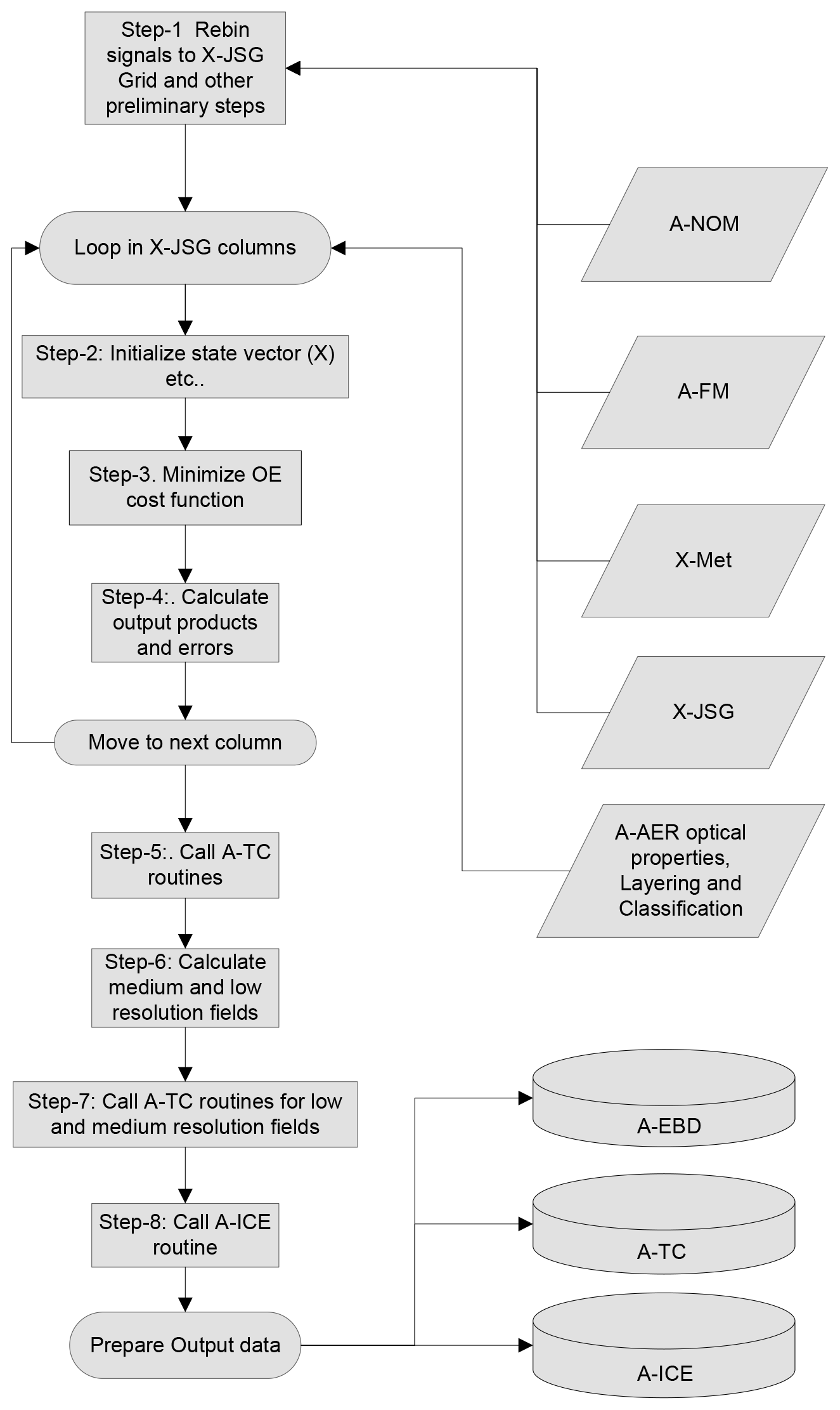
Step 1 is similar to the first step of the A-AER procedure. That is, the L1 ATLID signal is re-binned to the JSG resolution, and the auxiliary meteorological data are read and processed, etc. In addition, however, the A-AER results (layering structure, classification, retrieved extinction and lidar ratios, error estimates, etc.) are also read in this step.
Step 2 involves the setup of the OE inversion using the following steps.
-
For the lidar ratio elements of xa and their associated error estimates, A-AER-supplied values are used for layers when available.
-
For layers where A-AER could not derive a valid quantitative lidar ratio, a priori values based on the A-AER classification (e.g., ice cloud, water cloud, aerosol) are used.
-
The per-layer effective area sizes and associated a priori uncertainties are based on the A-AER classification. For ice clouds a temperature-dependent parameterization can be used (see Sect. 2.3.2).
-
The starting values for the extinction elements of the state vector are taken from A-AER when valid. Otherwise, they are based on either the layer-averaged scattering ratio and the a priori lidar ratio when valid or fixed values depending on the classification.
Once the OE problem has been set up, within step 3 the cost function is minimized using a version of the well-known Broyden–Fletcher–Goldfarb–Shanno (BFGS) quasi-Newton numerical minimization procedure (Press et al., 2007). The errors in the retrieved state vector (step 4) are computed following the procedure outlined in Sect. 15.5 of Press et al. (2007).
Once all the columns have been processed, the A-TC procedure is called to assign a classification to each layer (step 5). The A-TC classification procedure is described in Sect. 2.2 and 2.3 of Irbah et al. (2023). In step 6, the medium- and low-resolution fields are formed. Here the extinction, backscatter, and depolarization values are horizontally smoothed to medium and low resolutions. The smoothing is guided by the weak-feature mask (the complement of the strong-feature mask; see steps 2 and 7 of the A-AER procedure described in Sect. 2.2) modified to exclude E-EBD extinction values above an adjustable threshold and excluding any water cloud pixels. Medium resolution is set to default to 40 km and low resolution is set to a default of 150 km. These settings are adjustable and will be re-visited when in-flight ATLID data are available. For pixels not covered by the weak-feature mask, the high-resolution single JSG column values are used (i.e., the high-resolution results are merged with the low and medium fields). Using the merged low and medium fields, the A-TC classification routines are then called to generate the low- and medium-resolution classification fields (step 7). Lastly, the A-ICE product variables are calculated (see Sect. 2.3.2).
2.3.2 A-ICE
A-ICE is used to supply estimates of the ice water content (IWC) and effective particle radius using parameterizations supplied with retrieved extinction values and the atmospheric temperature. One of two options can be specified. The two approaches used are based on Heymsfield et al. (2005) and Heymsfield et al. (2014), respectively. The exact coefficients used in each approach are configurable and may be adjusted based on the experience with actual EarthCARE data. IWC and effective radii estimates are produced for all pixels identified as being ice in the A-TC product (Irbah et al., 2023).
In this section, the application of A-PRO to the three main EarthCARE test scenes (Qu et al., 2023; Donovan et al., 2023) will be presented and discussed. Here the focus is on the retrieved optical properties (extinction and lidar ratio); however, target classification results (A-TC) are also presented. For each of the three scenes (Halifax, Baja, and Hawaii) overall results are presented, and a few extracts are presented in detail. More information is presented in Mason et al. (2023a), where the results of various EarthCARE L2 retrieval algorithms are compared with each other and the model truth. It should be noted, however, that the data shown in this paper (version 11) are not the same as the version used in (Mason et al., 2023a) (version 10). In general, the results shown here (being based on a more developed version of A-PRO) are superior but not dramatically so.
One of the aims of this section is to give the reader a feeling for the nature of the product that will be supplied to the community including the limitations and possible caveats. To this end, the sample retrievals have not been over-tuned to produce optimal results. For example, it would be possible to tune the priors to the model scenes (e.g., lidar ratios, FMSp, Ra, η) to closely match the three scenes. This is not done here since it is instructive to gain insight into the relative robustness of the various retrieved variables in different circumstances given reasonable limited knowledge of the priors with respect to actual observations. For example, most of the ice clouds present in the test scenes have an associated lidar ratio of 30 sr; however, in these retrievals, an a priori value of 25 sr with a relative uncertainty of 20 % is used. The values of FMSp are also fixed and were not tuned; these were set based on idealized offline simulations (e.g., Appendix B) that were conducted independently of the main test scene construction process. As a result, bias differences from the model truth are to be expected. These differences will help guide investigations that will be conducted post-launch.
3.1 Halifax
The attenuated co-polar Mie, Rayleigh, and cross-polar backscatter signals and the corresponding A-FM feature mask (van Zadelhoff et al., 2023b) for the Halifax scene are shown in Fig. 7. These fields, along with the X-JSG and X-MET products (Eisinger et al., 2024), form the inputs for A-PRO. The particle extinction products produced by A-PRO corresponding to the inputs shown in Fig. 7 are shown in Fig. 8. The black regions are regions flagged as being not valid (e.g., attenuated or otherwise invalid); the vertical black strip is the result of a gap in the simulated lidar signals after re-binning to the JSG. In Fig. 8, the differences between the different products can be seen. Compared to the A-EBD fields, the A-AER estimate is the smoothest; however, no extinction estimates flagged as being valid are generated for the strong signals, e.g., clouds. For the A-EBD estimates it can be seen that the aerosol and thin ice cloud areas become smoother as the horizontal resolution decreases; however, the cloud extinction regions are not smoothed (see the last step described in Sect. 2.3.1).
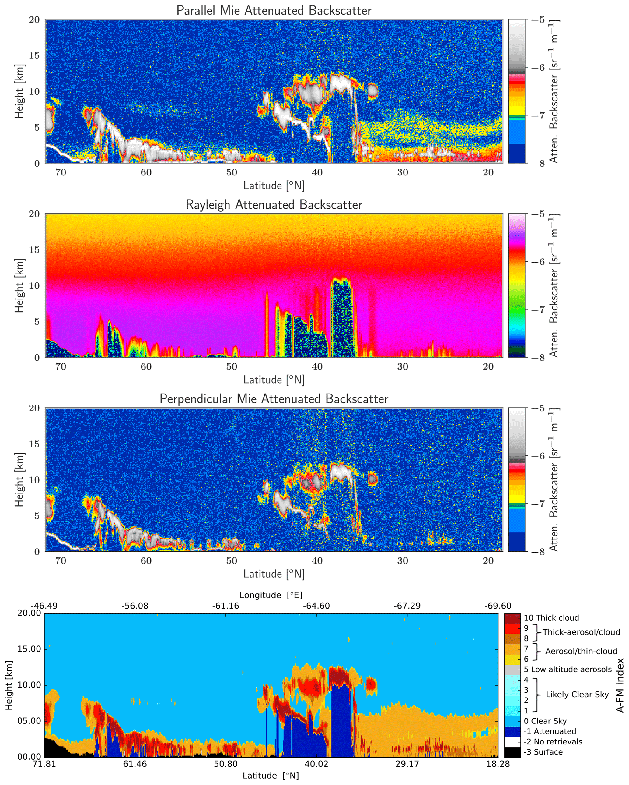
Figure 7Simulated Mie, Rayleigh, and cross-polar attenuated backscatter for the Halifax scene and the A-FM L2 feature mask.
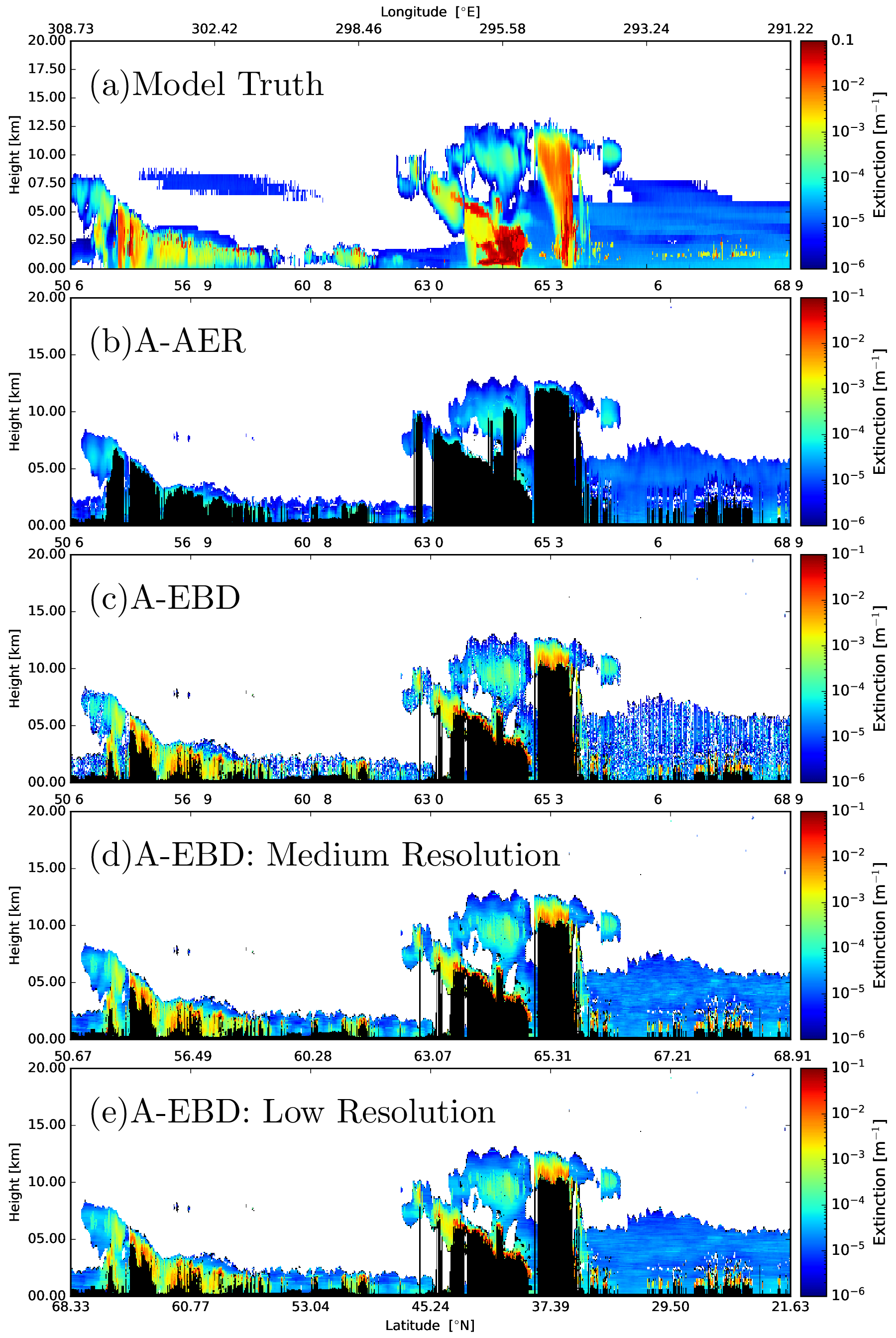
Figure 8Model truth extinction for the Halifax scene and the corresponding A-AER and A-EBD products. Here “medium” resolution is 50 km, while “low” resolution corresponds to 100 km.
Two example regions of the Halifax scene extinctions results are presented in more detail within Fig. 9. Here the retrieved extinction is compared to the model truth for a representative high-altitude ice cloud region and an aerosol region. In the profile plots of the retrieved extinction (αr) shown in the left part of Fig. 9b and c, the light blue regions correspond to the average estimated uncertainty in a relative sense, i.e.,
which is consistent with the logarithmic nature of the state vector used in the retrievals. The black lines represent the estimated error of the average profiles, i.e.,
where N is the number of samples contributing to the average.
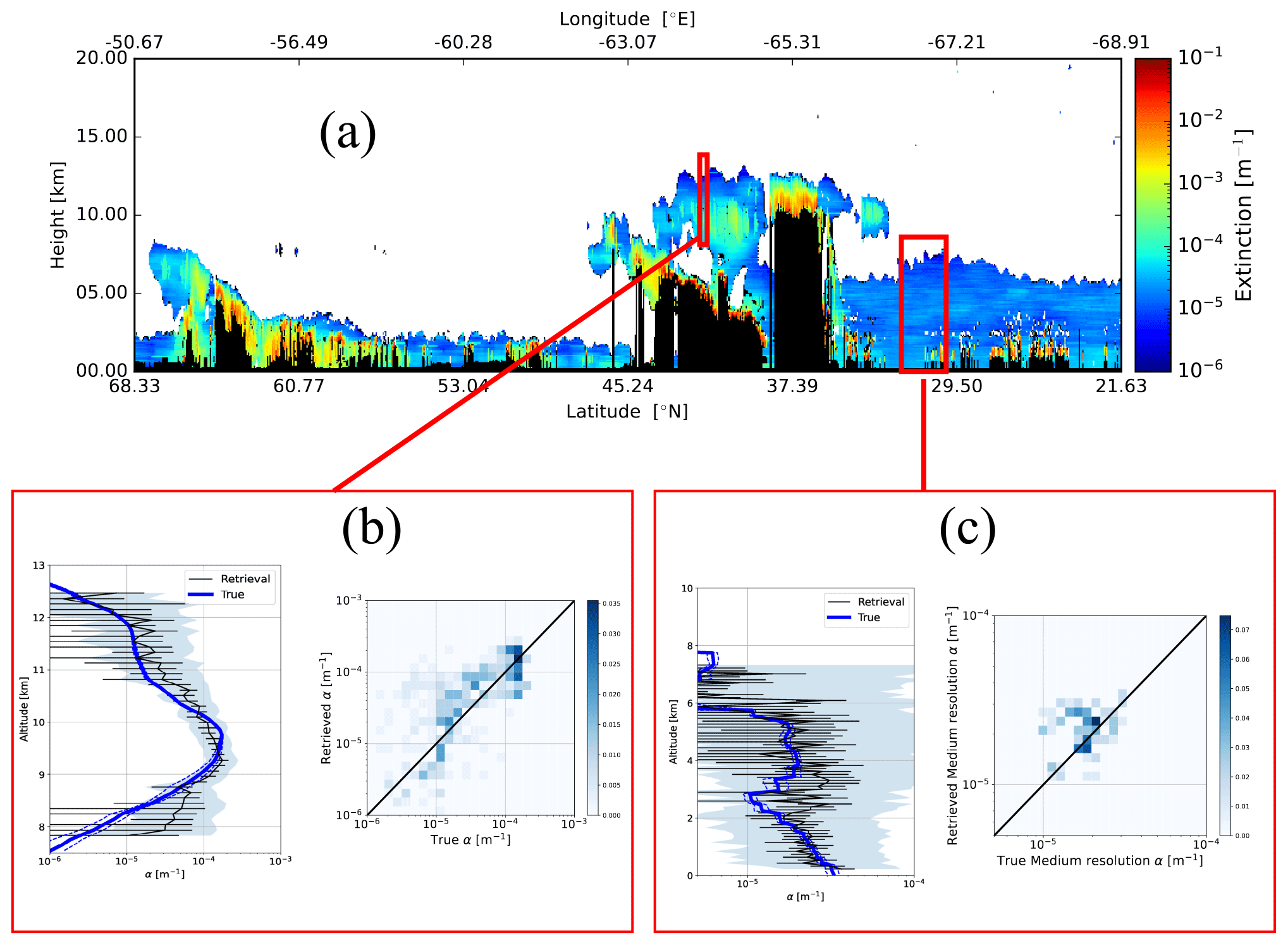
Figure 9Low-resolution retrieved extinction for the Halifax scene (a) and two representative average profiles. Panel (b) corresponds to a 10 km horizontal average of the A-EBD high-resolution extinction profiles and the corresponding model truth extinction profiles. Panel (c) corresponds to a 50 km horizontal average. The solid blue lines represent the average model truth, and the dashed blue lines delineate the ± the model truth standard deviation region. The solid black line represents the average retrieved extinction, the shaded light blue region shows the average relative uncertainty, and the error bars represent the uncertainty of the mean retrieved profile. The color scale assigned to the true vs. retrieved histogram plots corresponds to the normalized number of counts in each 2D histogram. The histograms were constructed using the medium-resolution outputs in the respective windows and not the horizontally averaged data (which are displayed in the associated profile plots.)
The sample ice cloud region (Fig. 9b) shows that on the 10 km scale the extinction values above 10−2 km−1 are accurately retrieved in this case (e.g., within a factor of 1.5), albeit with a low estimated precision. In the more attenuated areas of the cloud at lower altitudes (e.g., below 8.75 km), the accuracy and precision degrade due to worse SNR and the imperfect correction of MS effects. The second region (Fig. 9c) corresponds to a cloud-free aerosol case. Here it can be seen that on the 50 km−1 scale that extinction values above 10−2 km−1 are retrieved with an accuracy of about 50 %.
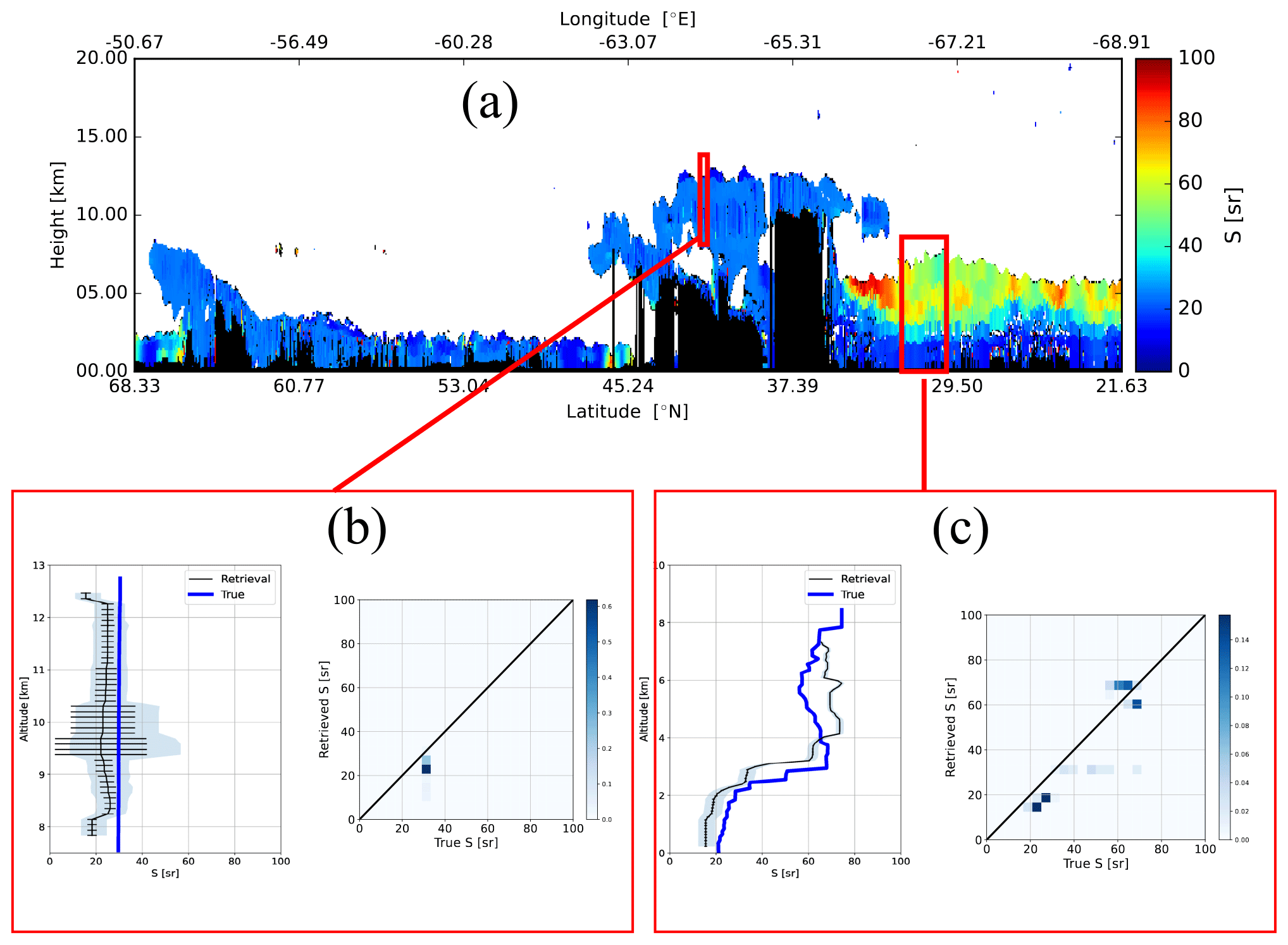
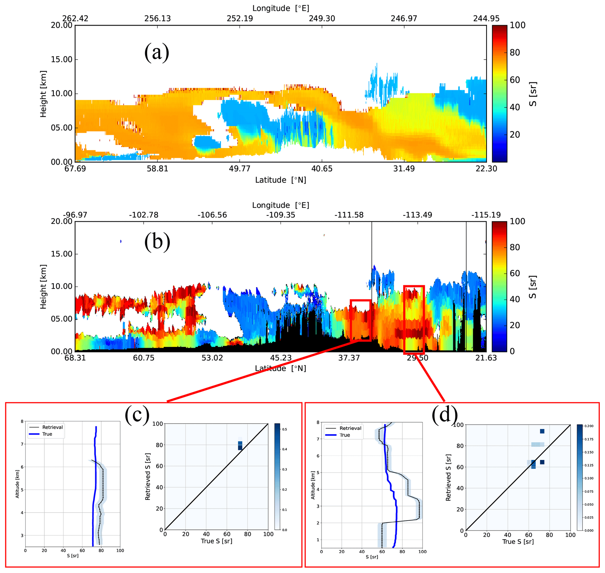
The lidar ratio retrievals corresponding to Figs. 8 and 9 are shown in Figs. 10 and 11, respectively. Here the fact that S is only retrieved per layer is evident (see the lower-right panel of Fig. 11). In Fig. 10 it can be seen that the A-AER estimates for the cloud aerosol are generally too low (15–20 sr vs. 25 sr for the model truth). This is roughly consistent which may be expected due to the limitations of correcting for multiple-scattering effects (see the discussion in Sect. B4). In the EBD optimal-estimation retrieval, the particle size is an element of the state vector, and a fuller treatment of multiple scattering is possible; thus, EBD generally retrieves lidar ratios that are closer to the model truth. Referring to Fig. 11, it can be seen that the retrieved lidar ratios are within about 10 %–15 % for the cirrus case. For the aerosol section presented in Fig. 11 (where multiple scattering is less important), the retrieved lidar ratios are generally within 10 %, and as a result there is not such a large difference between the AER and EBD retrievals.
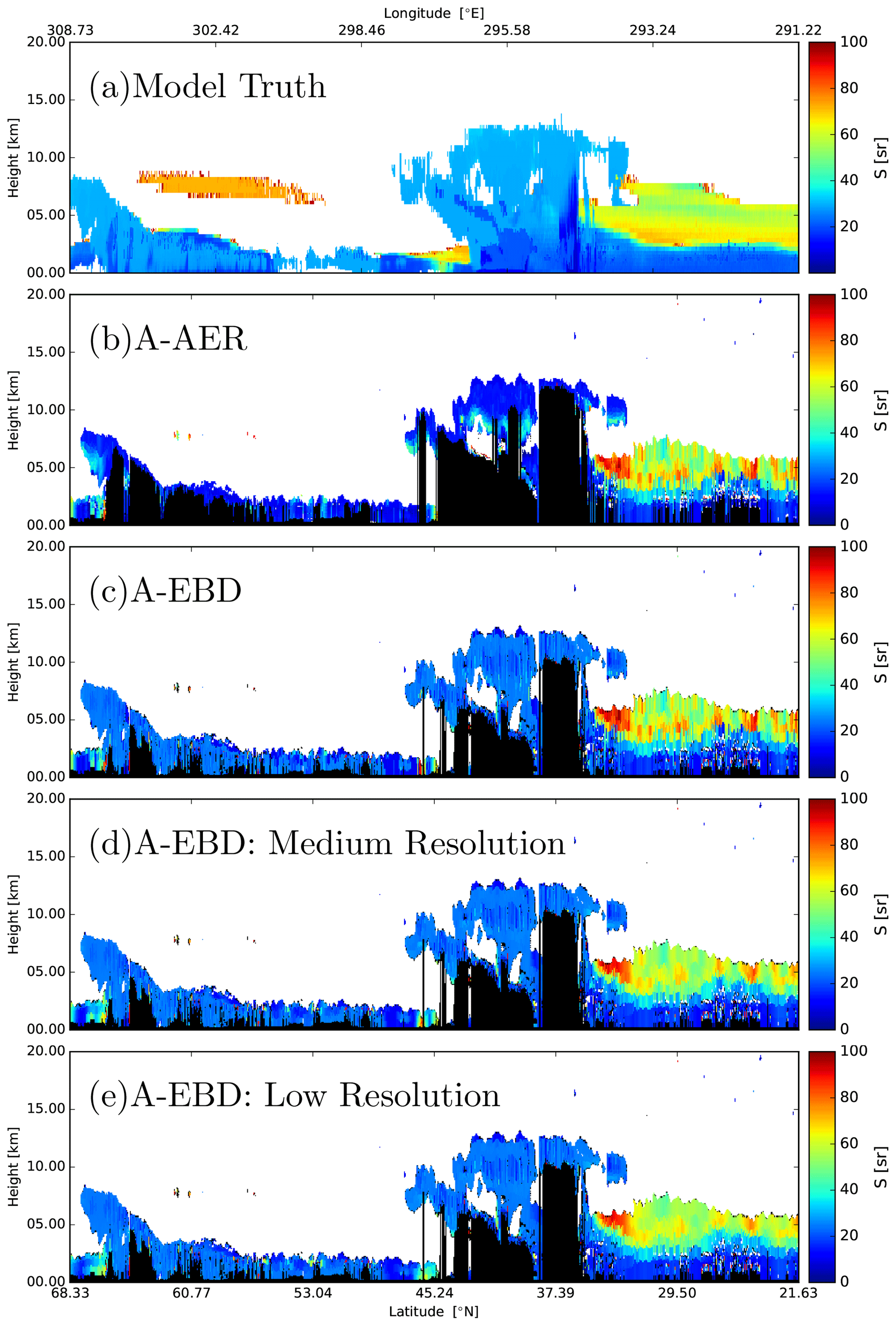
Figure 10Model truth lidar ratio for the Halifax scene and the corresponding A-AER and A-EBD products. Here “medium” resolution is 50 km, while “low” resolution corresponds to 100 km.
Within Figs. 10 and 11 it may be observed that the highest estimated values of the lidar ratio occur in the aerosol layer at around 32.5° N. This is even clearer in Fig. 12, where it can be seen that the anomalously high estimated lidar ratio leads to a misclassification of the aerosol type. This anomalous region coincides with the presence of a semi-transparent ice cloud present between about 8 and 10 km, and this is examined in more detail in Fig. 13. Referring to Appendix B, this is an example of the decaying multiple-scattering tail beneath clouds influencing the signals below. Figure 13g–k show that the Mie and Rayleigh attenuated backscatters are indeed well fitted and that the extinction is generally accurately retrieved (albeit with large relative estimated uncertainty); however, the retrieved lidar ratios exhibit large differences from the model truth. These errors are largely the result of the difficulty in fitting the decaying tail and the use of fixed values for the fMSp factors. This observation points to an avenue of inquiry once ATLID observations are available. In particular, if similar features in actual ATLID retrievals are found below semi-transparent cloud layers, then it may be necessary to refine the setting to fMSp, e.g., by including it in the state vector or parameterizing it as a function of multiple-scattering ratio and particle size and type. The graphs in Fig. 13a–f (the “Platt's approach” panels) are used to illustrate a related point. Namely, not allowing for the occurrence of tails in the forward model leads not only to somewhat higher retrieved lidar ratios but also to much higher retrieved extinction values below the ice cloud.
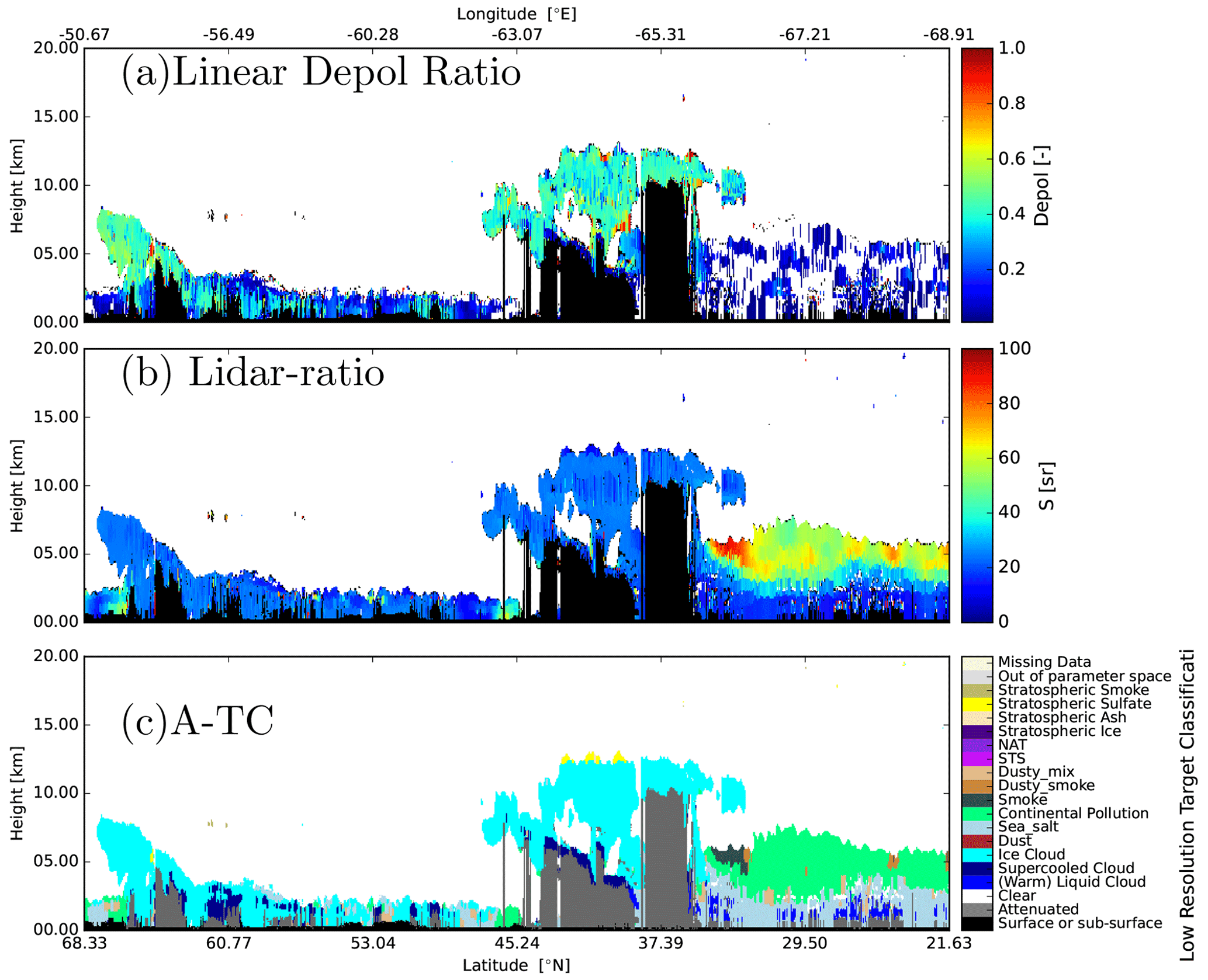
Figure 12(a) Low-resolution particulate depolarization ratio, (b) retrieved low-resolution lidar ratio, and (c) the corresponding A-TC classification field.
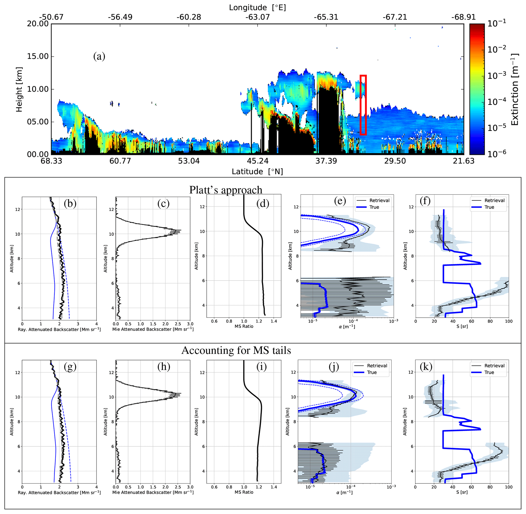
Figure 13(a) Retrieved low-resolution extinction. (b) Average Rayleigh attenuated backscatter for the indicated (10 km horizontal) interval (black line), the forward-model fit (dashed grey line), the corresponding single-scatter Rayleigh attenuated backscatter (solid blue line), and the Rayleigh clear attenuated backscatter profile. (c) Average Mie attenuated backscatter for the indicated interval (black line) and corresponding forward-model fit (dashed grey line). (d) Ratio of total (multiple scattering plus single scattering) to single-scattering return for the Rayleigh backscatter. (e) Average retrieved extinction profile and associated standard deviation profile (black lines) and average model truth extinction profiles (solid blue line). (f) Retrieved lidar ratio corresponding to (e). The dashed blue lines correspond to plus and minus the model truth standard deviation profile. Panels (b)–(f) correspond to retrievals conducting using Platt's approach, while panels (g)–(k) correspond to retrievals conducted using the default multiple-scattering (Platt + tails) model.
3.2 Baja
The attenuated co-polar Mie, Rayleigh, and cross-polar backscatter signals and the corresponding A-FM feature mask (van Zadelhoff et al., 2023b) for the Baja scene are shown in Fig. 14. The corresponding model truth extinction, the retrieved low-resolution extinction field, and details of two selected areas are shown in Fig. 15. The two sections selected here are both free of cloud with no overlying semi-transparent cloud layers. The extinction values are generally retrieved to within 10 %–15 %. The corresponding lidar ratio results are shown in Fig. 16. Here it can be seen that the lidar ratios are retrieved usually within about 10 %–20 %.
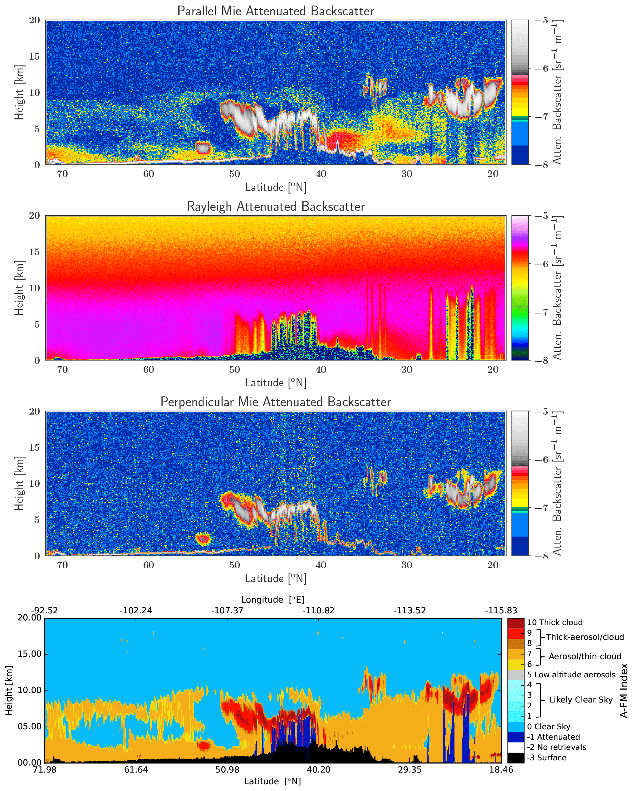
Figure 14Simulated Mie, Rayleigh, and cross-polar attenuated backscatters for the Baja scene and the corresponding A-FM L2 feature mask.
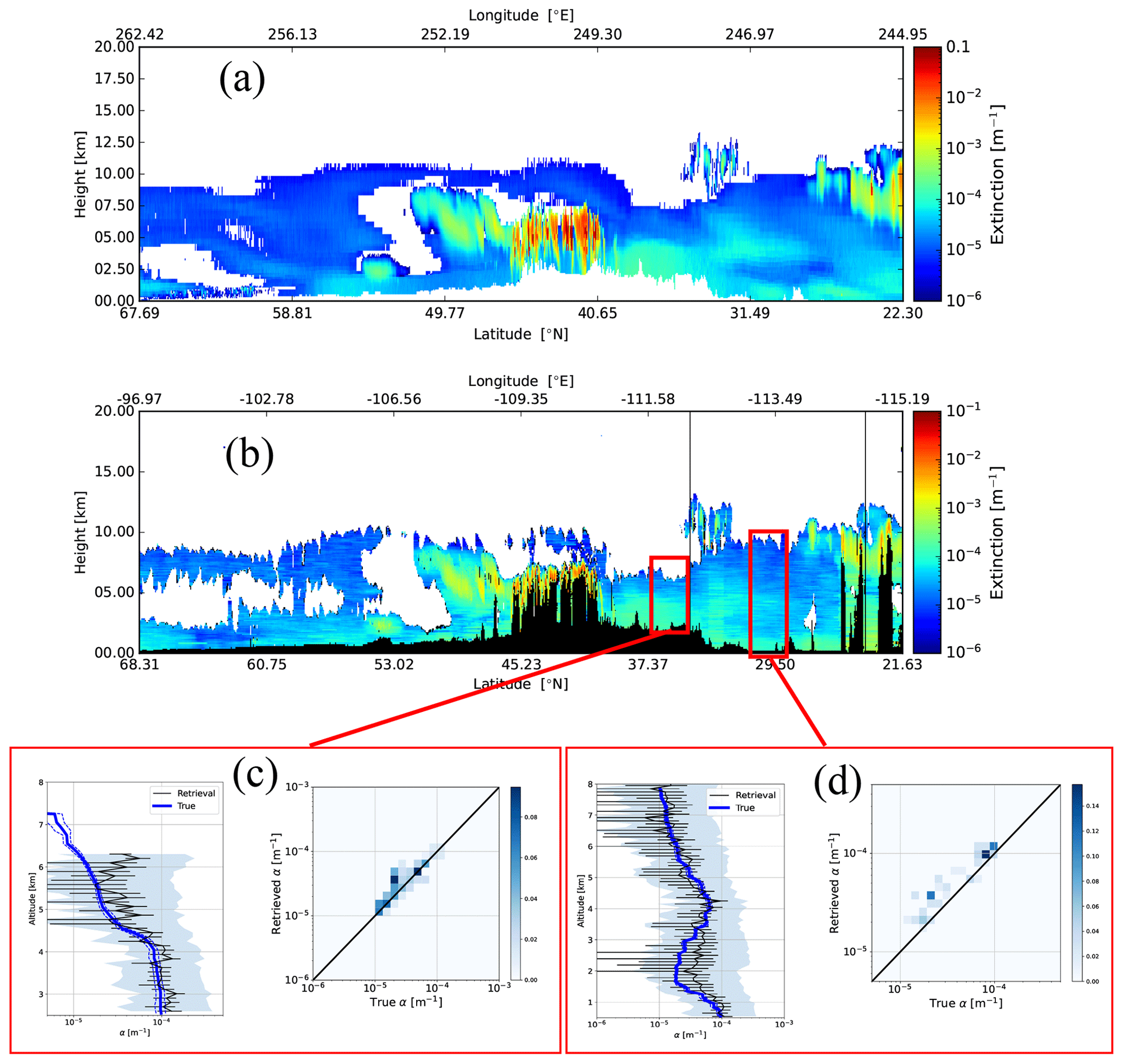
Figure 15Model truth extinction (a) and low-resolution retrieved extinction for the Baja scene (b) and two representative average retrieved profiles (c, d) for the indicated intervals. Panels (c) and (d) correspond to the low-resolution (100 km resolution) and corresponding model truth extinction profiles.
A detailed view of an ice cloud region in shown in Fig. 17. Here it can be seen, consistent with what was observed in general for the Halifax scene, that the extinction profile is well retrieved (within 5 %–10 %); however, the lidar ratio is underestimated (especially below 4 km). This is likely in part due to fMSp not being set optimally. Even though below 4 km the ice cloud is giving way to optically thinner and smaller particle aerosol, the multiple-scattering ratio is still high (see Fig. 18); thus, it is important to treat fMSp accurately even if the target in question possesses a small effective radius and is not optically thick if it underlies a layer that generates a significant amount of multiple-forward-scattered light.
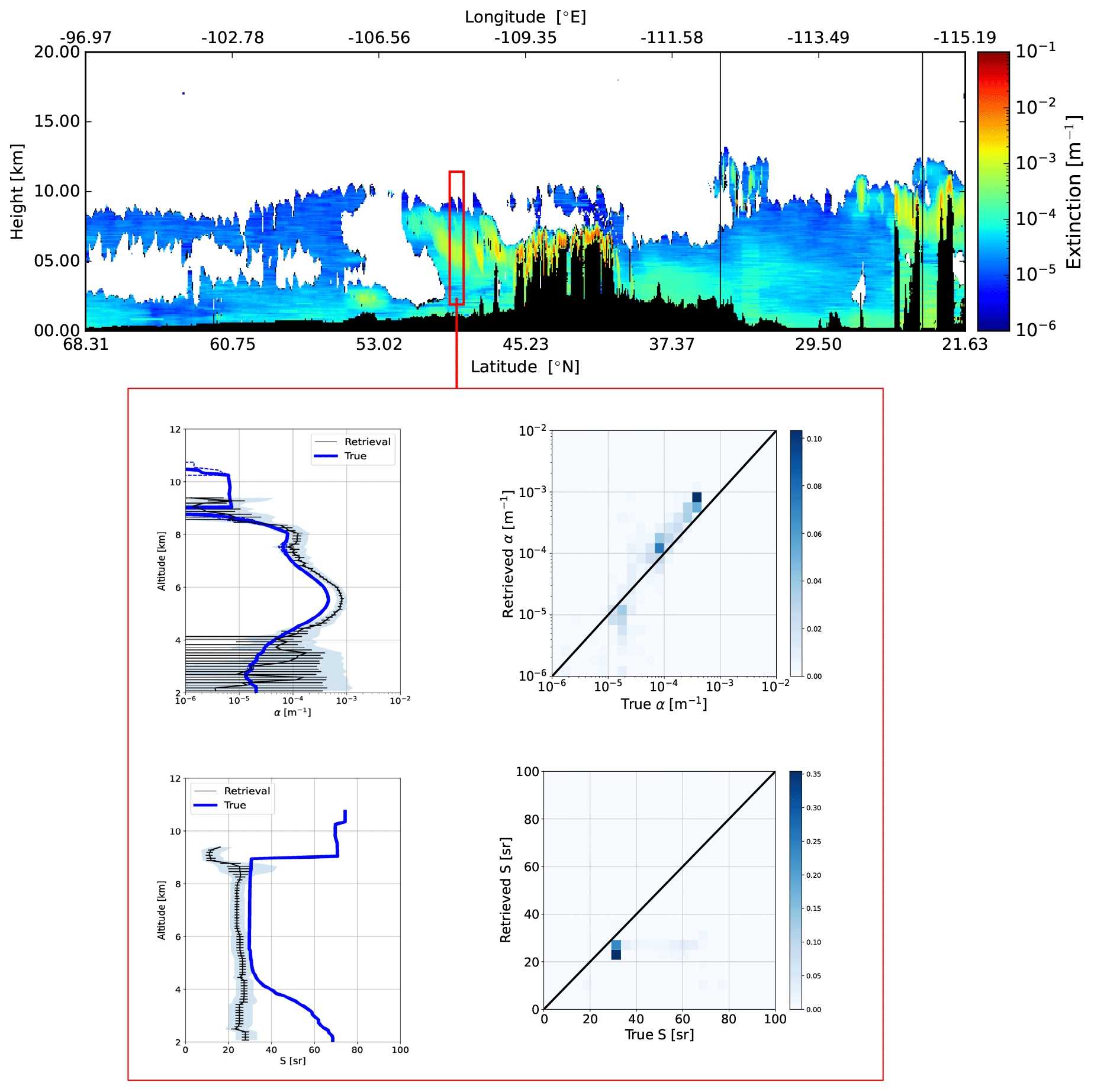
Figure 17Low-resolution retrieved extinction for the Baja scene (top panel). The bottom panels correspond to the indicated 10 km horizontal region.
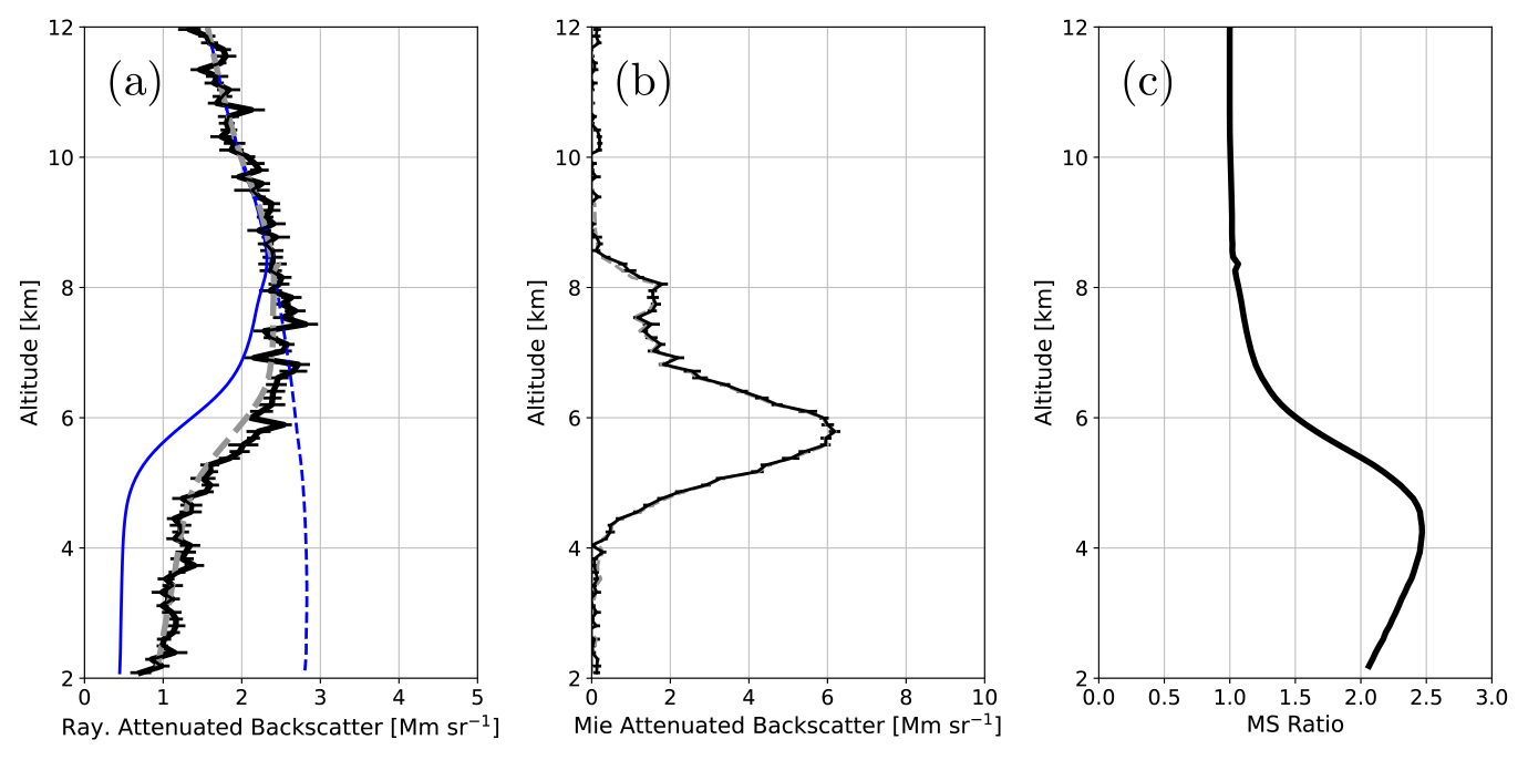
Figure 18(a) Average Rayleigh attenuated backscatter for the interval indicated in Fig. 17 (black line), the forward-model fit (dashed grey line), the corresponding single-scattered Rayleigh attenuated backscatter (solid blue line), and the Rayleigh clear attenuated backscatter profile. (b) Average Mie attenuated backscatter for the indicated interval (black line) and corresponding forward-model fit (dashed grey line). (c) Ratio of total (multiple scattering plus single scattering) to single scattering return for the Rayleigh backscatter.
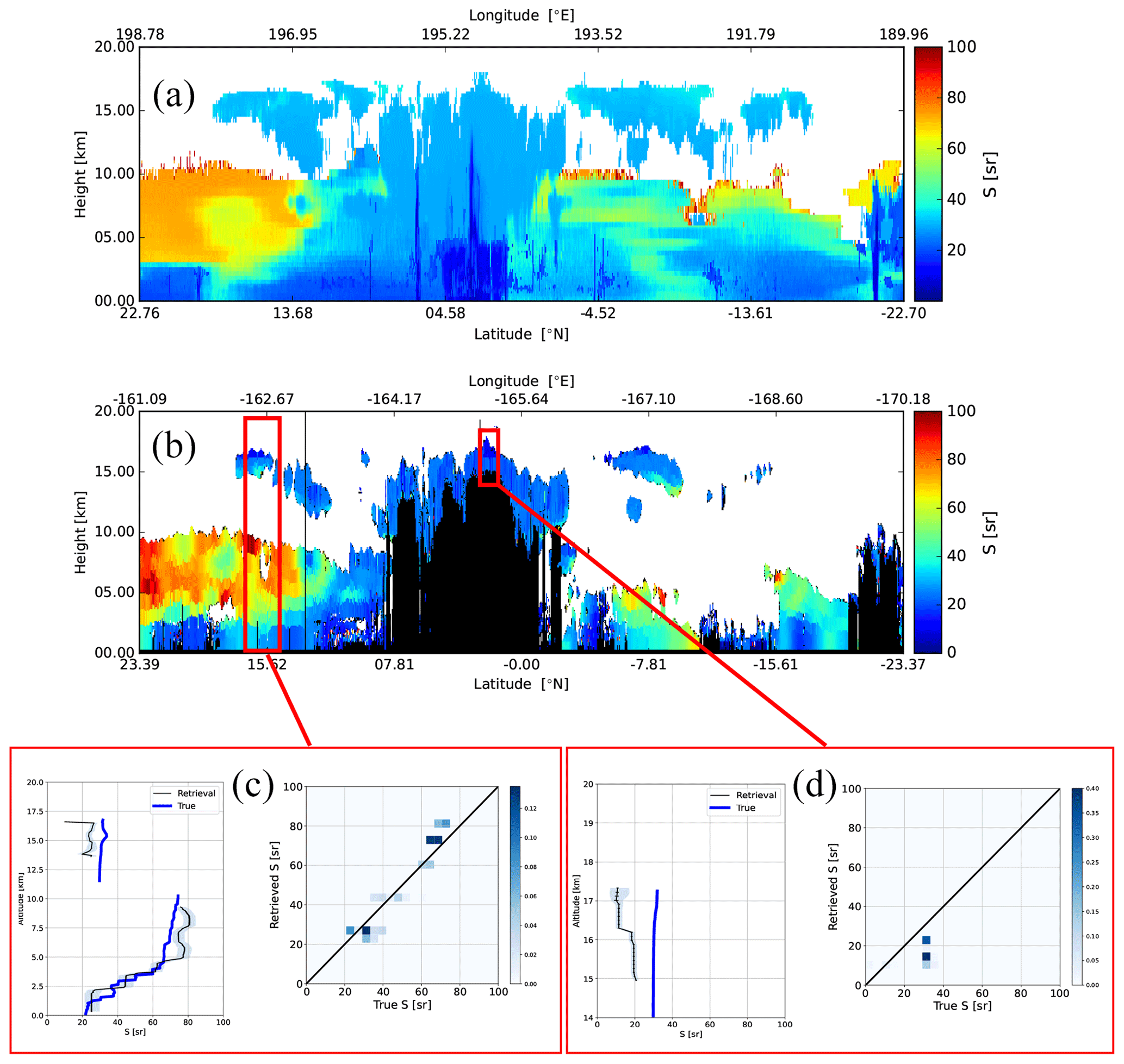
3.3 Hawaii
The attenuated co-polar Mie, Rayleigh, and cross-polar backscatter signals and the corresponding A-FM feature mask for the Hawaii scene are shown in Fig. 19. The corresponding model truth extinction, the retrieved low-resolution extinction field, and details of two selected areas are shown in Fig. 20. The extinction accuracy is seen to be consistent with the other two previously discussed scenes. Referring to the corresponding lidar ratio details shown in Fig. 21, it can be seen for the area highlighted in Fig. 21c, in this case an area where the upper layer ice cloud is optically quite thin, that this does not seem to greatly affect the retrieval of underlying lidar ratio. For the selected optically thick ice cloud area shown in Fig. 21d, the extinction profile is well retrieved nearly up to the point of complete attenuation; however, as was seen before, the retrieved lidar ratio is biased low.
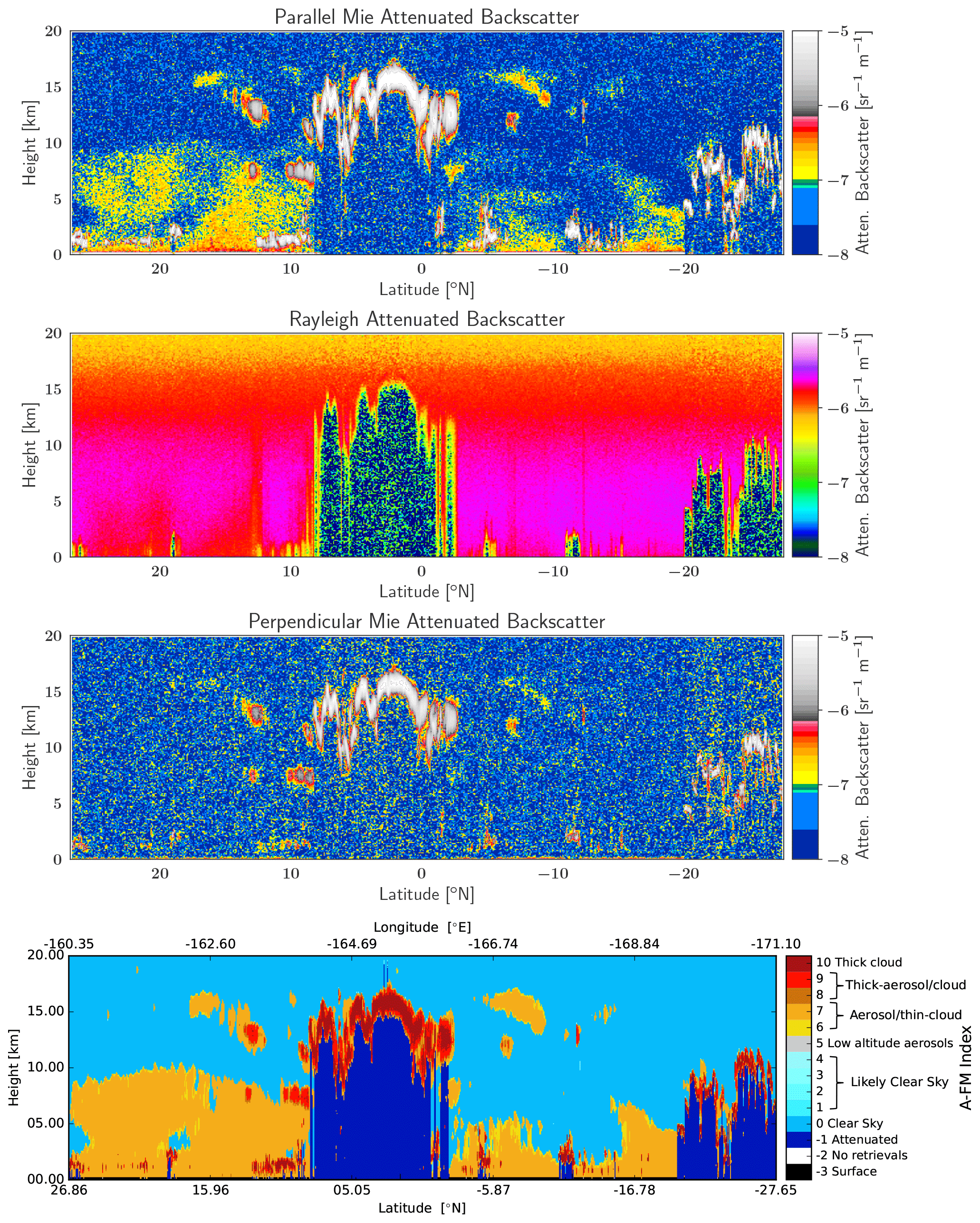
Figure 19Simulated Mie, Rayleigh, and cross-polar attenuated backscatters for the Hawaii scene and the A-FM L2 feature mask.
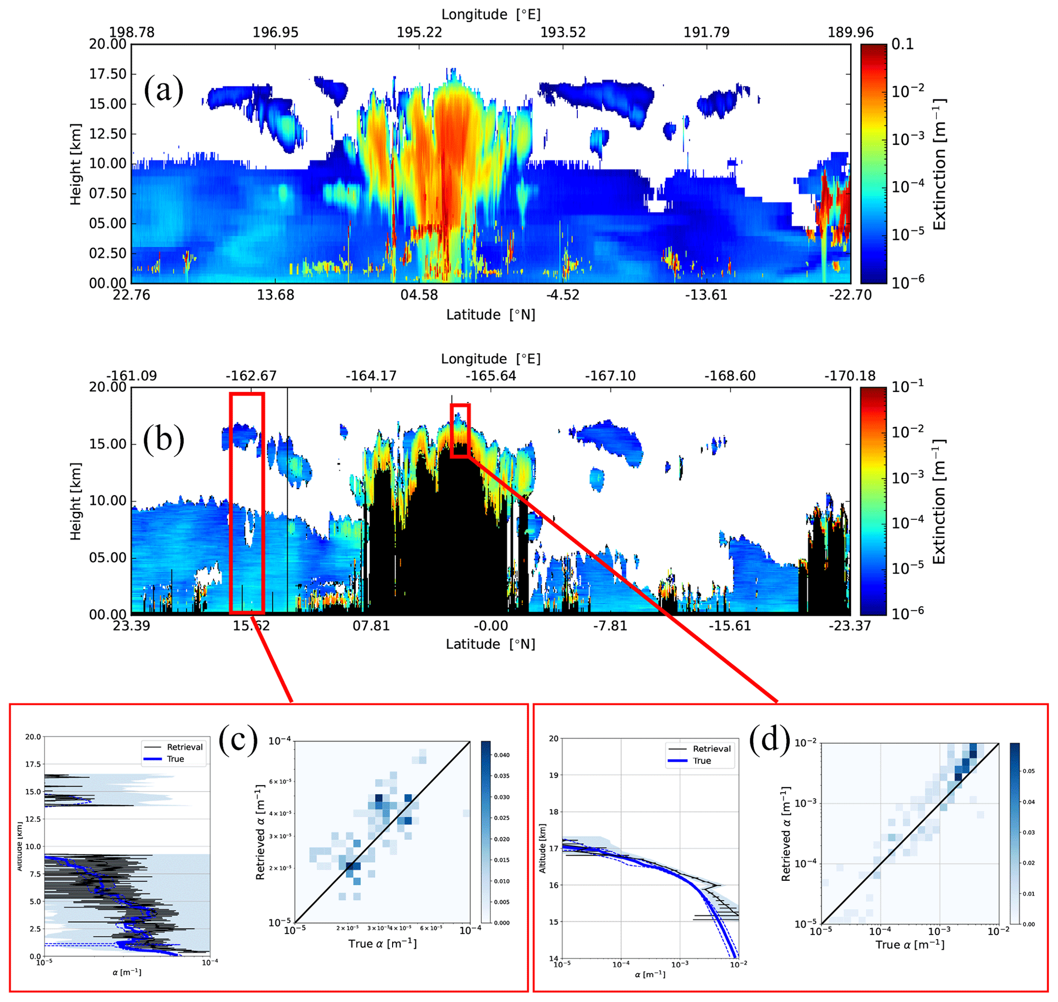
Figure 20Model truth extinction (a) and low-resolution retrieved extinction for the Hawaii scene (b) and two representative average retrieved profiles (bottom panels) for the indicated intervals. Panel (c) corresponds to the low-resolution (100 km resolution) and the corresponding model truth extinction profiles, while panel (d) corresponds to a 10 km horizontal interval.
The accurate retrieval of aerosol and cloud properties from space-based lidar is a challenging endeavor, even when the extra information provided by an HSRL system is exploited. Accounting for the generally low SNR ratios involved coupled with the need to respect the structure of the aerosol and cloud fields being sensed presents particular challenges. A-PRO addresses these challenges by implementing a multi-scale approach, resulting in a viable practical approach for both clouds and aerosols.
In this paper, a detailed overview of the A-PRO processor has been presented. The focus has been purposely limited to the extinction and lidar ratio retrievals. For a more complete picture, the interested reader should also consult Irbah et al. (2023), as this is where the layer determination and classification procedures are described in detail.
The development of the A-PRO processor has mainly been based on synthetic data (though a “cousin” algorithm, called AEL-PRO, has been applied to Aeolus data as in Straume et al., 2020, which is the subject of another paper, i.e., Wang et al., 2024), and further refinements and extensions will no doubt be made when actual ATLID observations are available. One of the issues that has been noted and indeed highlighted within this paper is the potential difficulty in properly accounting for multiple-scattering effects. Retrievals below higher scattering layers can be affected by the presence of “tails”, which can be difficult to accurately model. Further, it is likely that a more comprehensive investigation and treatment of the role of anisotropic backscattering of multiple-scattered light (i.e., issues surrounding the fMsp factor) is required. It seems that in situations where multiple scattering is important the extinction is often more robustly retrieved than the lidar ratio. This is not surprising given that the extinction information is closely related to the Rayleigh signal profile, which can be modeled independently of fMsp. The modeling of the Mie backscatter signal involves both S and fMsp, and this extra degree of freedom can create additional uncertainty when retrieving the backscatter (or equivalently the lidar ratio). Based upon further simulation-based studies, as well as actual ATLID observations, this issue will be revisited and may result in extensions to the A-PRO procedures (i.e., parameterization of fMsp or including fMsp in the state vector of the A-EBD optimal-estimation algorithm).
A1 Standard estimation of lidar ratio, extinction, and backscatter
Neglecting multiple-scattering effects for the time being using Eq. (8) and using the fact that we have
Further, using Eq. (9) and using the fact that
where the Rat superscript is used to denote the fact that the ratio between the observed Rayleigh extinction-corrected attenuated Rayleigh backscatter and the unattenuated Rayleigh backscatter is being calculated. Fhv is used to denote the masked vertical and horizontal smoothing operation, and τRay is the Rayleigh optical depth from the top of the atmosphere to the height in question. For simplicity reason the range dependence is not written explicitly here.
If we assume that the action of the smoothing operation can be ignored then by taking the range derivative of Eq. (A2) and re-arranging it yields an expression for the particulate extinction, i.e.,
and dividing Eq. (A2) by Eq. (A1) yields an expression for the particulate backscatter coefficient, i.e.,
Dividing the two previous equations then yields an expression for S, i.e.,
Deriving the extinction, backscatter, and the associated lidar extinction-to-backscatter ratio using any approach related to that just outlined in which the signals are smoothed either explicitly or implicitly can lead to inaccurate results for the determination of S, e.g., near the edges of clouds or aerosol regions. This is due to the fact that the extinction information (which is related to the signal derivative) and the backscatter information are linked to different vertical scales (i.e., the action of Fh,v cannot be ignored in the above derivation). In particular, the vertical derivative of the ATBs cannot be unambiguously linked to a single range bin but can only be assessed using two or more bins; however, the backscatter can be assessed, in principle, at the scale of a single range bin. This fundamental difference in the scale at which the extinction and backscatter information can be retrieved gives rise to undesirable edge effects. This problem can be made worse when vertical smoothing of the ATBs over a number of range gates must be applied in order to increase the effective SNR as is done here. In effect, applying the same smoothing strategy to both the Rayleigh and Mie ATBs, due to their dissimilar structure, does not result in the S ratio being preserved even in cases where no noise was present.
One of the uses of the S profiles within the A-AER is to help determine the layer structure (see steps 10–11 in Sect. 2.2), and spurious features in the S profile can give rise to spurious layers. In part for this reason, an alternation procedure was developed and implemented which tends to produce fewer edge effects in the S determination process. This procedure is described subsequently.
A2 Local forward-modeling-based estimation of S, extinction, and backscatter
An approach that attempts to limit the issues involved with spurious edge effects with S profile determinations is to perform a local forward-model fit, which in a sense puts the retrieved extinction and backscatter on the same scale. The basic idea is to find the best value of S over a vertical fitting window that, together with the conventionally derived backscatter profile, best predicts the observed Mie and Rayleigh ATB profiles.
As a starting point, the backscatter profile and extinction profiles and the subsequent values of S are determined using Eq. (A4). The algorithm them proceeds as follows.
- 1.
For the fitting window, the average backscatter is determined:
where itop and ibot are the range indices of the fitting window boundaries and N is the number of range gates in the fitting window.
- 2.
Using a specified value of S, the average particulate extinction within the fitting window is estimated, i.e.,
- 3.
The un-normalized predicted local profiles corresponding to and BM,hv are calculated as follows:
and
where , ro is the value of the range gate closest to the lidar within the fitting window, and ri is the range of the ith range gate within the fitting window.
- 4.
The local calibration factor (Cloc), which normalizes the profiles calculated in the previous step with respect to the observations, is then calculated, i.e.,
where the summation is carried out over the fitting window.
- 5.
The Chi-squared difference between the local forward-model fit and the corresponding observations, as well as its derivative with respect to S, is calculated, i.e.,
and
where
and
Here the error estimates (the σ term) are calculated using standard error propagation techniques based on the estimated random error in the observed Rayleigh and Mie attenuated backscatters.
- 6.
The value of S that minimizes χ2 is found numerically using the Secant method applied to . For the initial iteration, the values of S generated by the application of Eq. (A4) are used. The Secant iteration continues (looping back to step 5) until a maximum number of iterations is reached (usually set to 10) or successive values of S are within a set tolerance (e.g., 1 %).
- 7.
The uncertainty in the retrieved value of S is estimated using a scaled χ-squared approach, i.e.,
where is the minimum value of the cost function obtained in the previous step.
- 8.
Using the backscatter profile and S the extinction profile and its associated uncertainty are determined.
The procedure described above is numerically based, but it is fast and does have an advantage compared to more conventional methods; in particular the S retrievals are better behaved near the edges of scattering layers. This is illustrated in Fig. A1, where the results of a simple idealized simulation are presented. Here a simple two-layer aerosol field was used to simulate Rayleigh and Mie attenuated backscatter profiles. Figure A1b shows the noiseless ATB signals both at the native ATLID resolution of 100 m and at a retrieval resolution of 300 m; it is clear that the smoothing affects the Mie ATB signals more than the corresponding Rayleigh profile. This is further reflected by the large oscillation in the extinction-to-backscatter ratio retrieved using the conventional approach. The local forward-modeling approach yields generally superior results near the layer boundaries.
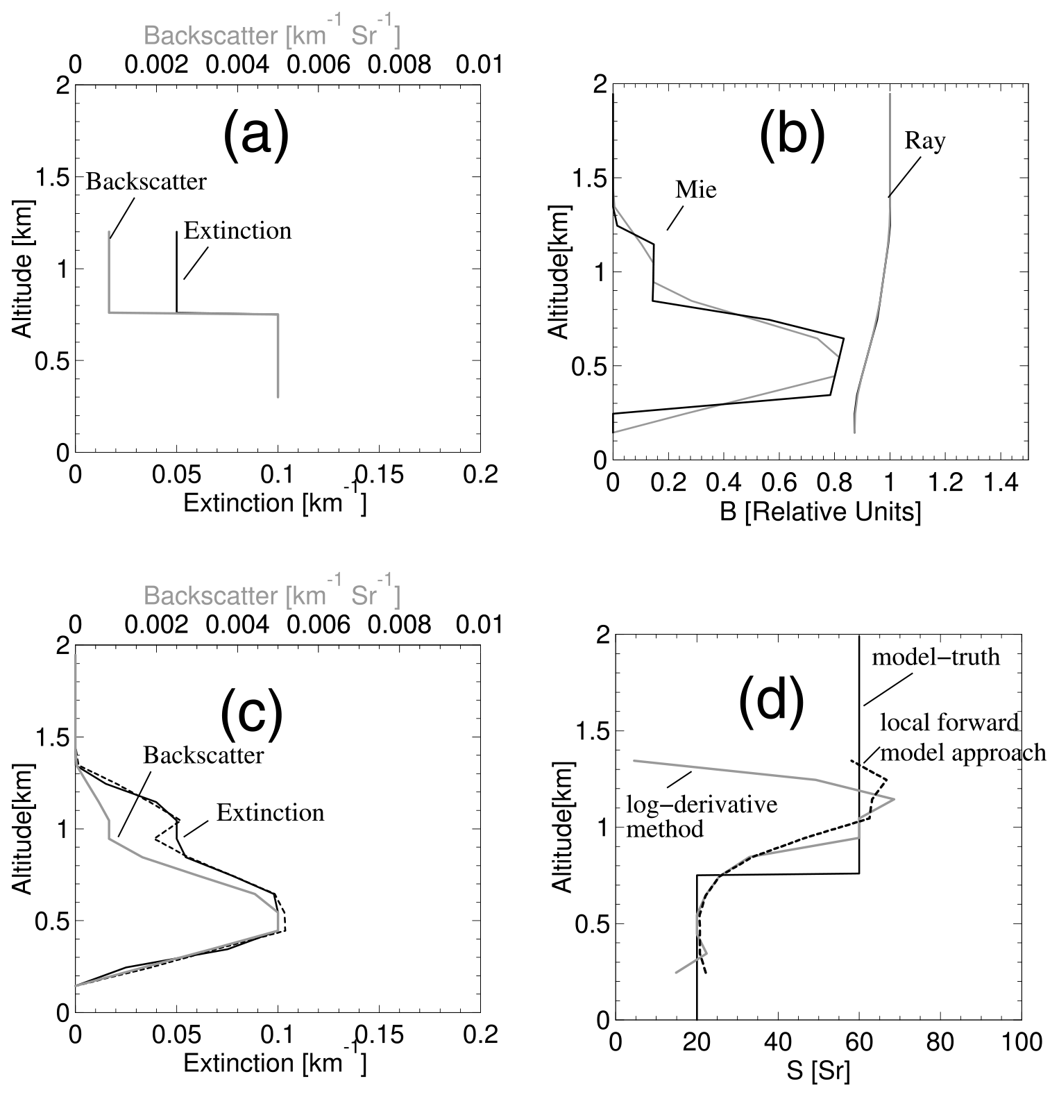
Figure A1(a) Profiles of model truth extinction and backscatter. (b) Attenuated Rayleigh and Mie backscatter profiles at 0.1 km resolution (black) and 0.3 km (grey). (c) Retrieved backscatter (grey line) and retrieved extinction using the conventional log-derivative approach (solid black line) and the local forward-modeling approach (dashed black line). (d) The solid black line corresponds to the model truth extinction-to-backscatter ratio, the solid grey line represents the conventional log-derivative approach estimate, and the dashed black line corresponds to the result from the local forward-modeling approach.
The inversion of ATLID lidar signals requires a fast yet accurate treatment of lidar multiple scattering. Example simulated signal profiles for an idealized cirrus cloud are shown in Fig. B1. Here three different models of different complexity have been applied, namely Monte Carlo (MC), the reduced extinction approach due to Platt (Platt, 1981), and the quasi-small-angle (QSA) (Hogan, 2006) and photon variance–covariance (PVC) methods (Hogan, 2008). The Monte Carlo results were calculated using the EarthCARE Simulator (ECSIM) lidar radiative transfer model (Donovan et al., 2015) and are considered the most accurate here. Here it can be seen that the QSA results are close to the MC results both within and below the cloud. Platt's approach performs well within the confines of the cloud but cannot follow the shape of the tails arising from the decay of the signal towards single-scattering levels below the cloud base.
Hogan's approach is accurate and orders of magnitude faster than MC calculations. However, it is still much slower than the corresponding single-scattering case. Platt's approach, on the other hand, is as fast as calculating the single-scattering return. In this work, a novel approach is developed that is between the approaches of Platt and Hogan in terms of complexity.
We first discuss Platt's effective extinction approach and discuss how this can be extended to handle the phenomenon of decaying tails.
B1 Platt's approach
Within Fig. B1 it can be noted that within the cloud the observed signal closely resembles a less attenuated version of the single-scattering signal. This is to be expected when the particles are large compared to the wavelength of the laser light, meaning that half the scattered energy is scattered forward in a narrow diffraction lobe and largely stays within the lidar receiver field of view. This result was noted by Platt (1976) and forms the basis of a simple method for accounting for multiple-scattering effects.
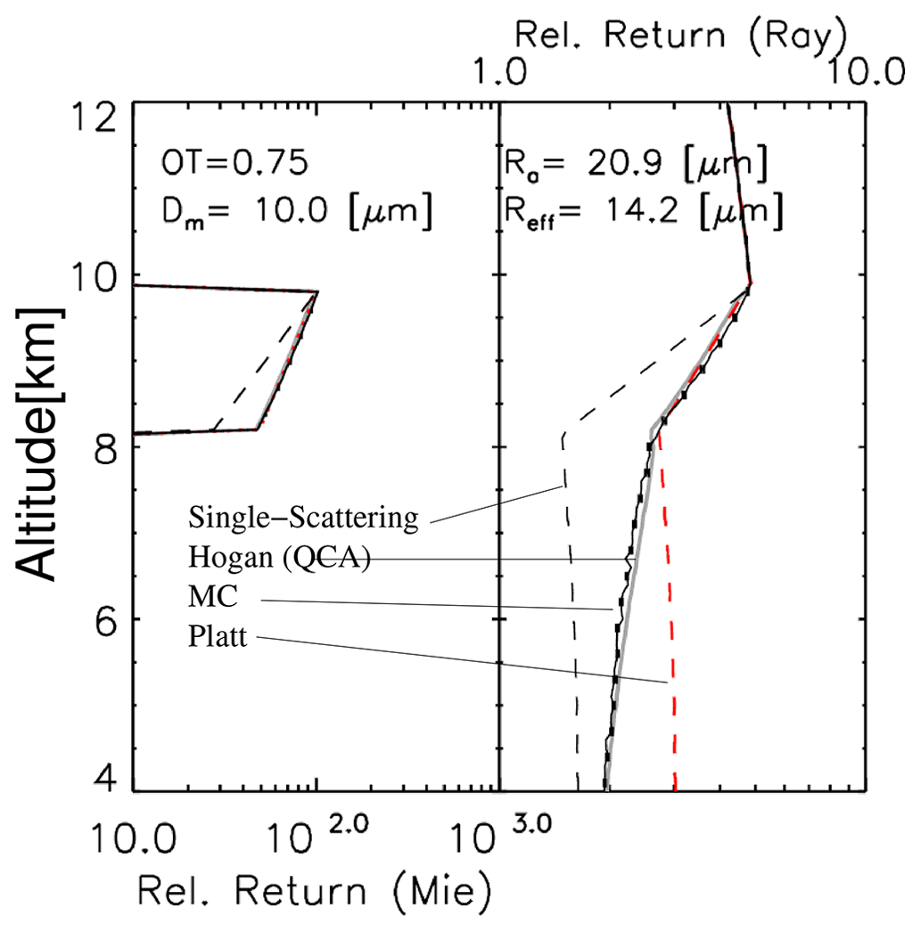
Figure B1Sample comparison between the ECSIM lidar Monte Carlo multiple-scattering model (Donovan et al., 2023), the analytical model due to Hogan and Battaglia (2008), and Platt's equation (Eq. B2) for an idealized single layer ice cloud of optical thickness (OT) of 0.75 and an effective radius of 30.7 µm. Mie co-polar (left) and Rayleigh channel co-polar (right) returns. The solid black line (with error bars) shows ECSIM results. The dashed black line shows single-scattering results. The solid grey line shows Hogan's model results for the true value of Ra. The red line shows Platt's equation.
We define
where Mp is the ratio of the total received power including all scattering orders (P) and the single-scattering power Pss. The variable ηp is the multiple-scattering effective extinction factor such that (1−ηp) is the fraction of scattered energy that remains within the lidar field of view (and thus behaves like it has not been scattered). If one then multiplies this expression by an expression for the single-scattering lidar attenuated backscatter, then Platt's multiple-scattering equation is recovered, i.e.,
B2 The origin of MS tails
As mentioned above, Platt's approach is fast but severely limited in cases where tails may be present. These tails are not due to temporal pulse stretching, which is associated with thick clouds (e.g., Hogan and Battaglia, 2008). The origin of the tails in question here can be simply explained. Referring to Fig. B1, within the cloud the low mean free path of the photons ensures that the multiple-scattered light that contributes to the detected signal tends to be confined to within the field of view of the lidar; however, the angular variance of the lidar beam will increase as it propagates downwards through the cloud with more and more photons undergoing scattering events.
At cloud base, the lidar beam emerges with an effective angular divergence that increases with the optical thickness of the cloud and decreases with the size of the cloud particles. This is due to that fact that the angular width of the cloud-phase function forward lobe increases with decreasing particle size, i.e.,
Below the cloud base the lidar beam will continue to propagate with a given divergence. However, the horizontal spread of the photons is no longer constrained by the presence of the cloud. As the beam continues to propagate downwards, depending on the lidar receiver footprint, more and more of the multiple-scattered photons will travel outside of the receiver cone. Though less pronounced, mainly due to the larger field of view, such tails can be found in CALIPSO observations.
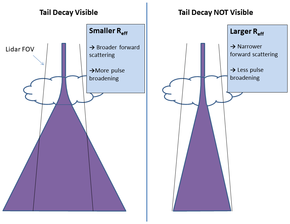
Figure B2Schematic depiction of the mechanisms behind the occurrence of decaying tails below scattering layers. Here the purple regions represent the broadened laser pulse extent.
B3 An extension to Platt's approach
Following the discussion in the previous section, it is apparent that the tails can be viewed as a decay of the signals towards single-scattering levels. Accordingly, we modify the form of the multiple-scattering ratio in Eq. (B1) to allow for such decays to occur, i.e.,
where (here assumed to be constant per atmospheric layer) and f(z) is the range-dependent multiple-scattering return signal fraction. Note that here we have replaced ηp with η for reasons of convenience, meaning that η is equal to the fraction of multiple-scattering light remaining in the field of view (instead of 1−ηp). Note that if η is equal to zero, then M(r)=1 (regardless of the values of f(z)) and no multiple scattering is detected. Also, if f(z) is equal to zero M(z)=1 (regardless of the values of η(z)) and f(z) is equal to 1, then Eq. (B4) reduces to Eq. (B1).
If we multiply Eq. (B4) by the single-scattering lidar attenuated backscatter expression, then
Determination of f(z)
To be useful, a means to determine the profile of f(z) must be established.
We start by considering the case of a physically thin scattering layer as schematically depicted in Fig. B3. If we assume that the beam has a Gaussian profile and the forward-scattering lobe of the effective layer-phase function is approximated by a Gaussian (Eloranta, 2005), then the divergence of the forward-scattered light will also be Gaussian with a divergence given by the convolution of the incoming beam divergence (θl) with the effective scattering forward lobe width (θSc) so that the effective width of the multiply scattering radiation emerging from the layer bottom is given by
By integrating the effective beam across the lidar field of view (FOV) the fraction of the light that remains within the FOV is given by
where ρt is the receiver telescope full-angle angular FOV, θl is the laser full-angle divergence, rsat is the satellite altitude, and r(zl) is the altitude of the scattering layer. This expression is only valid for a single thin scattering layer, and it is thus not so useful by itself. However, we can generalize this expression to the case of a general profile in a heuristic approximate fashion. A rigorous calculation would be involved and would result in a similar formalism as the QSA model of Hogan (2008). Here we will use the information present in the signal itself to calculate the effective f profile under general conditions. Since the observed signal itself contains information on the location and relative strength of the scattering at each level, we postulate the form
where B is the total observed attenuated backscatter. That is, we use the observed backscatter profile itself as a weighting factor to determine the effective profile. In the limit of a single thin scattering layer this expression yields the correct result.
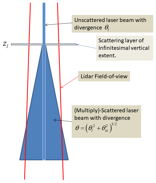
Figure B3Schematic depiction of the angular broadening experienced by a lidar pulse as it interacts with a physically thin scattering layer at altitude r(xl).
An example comparison between Monte Carlo calculations, Platt's approach, and the “Platt + tails” approach (Eq. B5) together with Eq. (B8) is shown in Fig. B4. Here a fitting procedure was used to find the best values of η and θSc for each of the two layers. It can be seen that the extended Platt approach provides a very good match to the MC results for the entire profile, whereas the normal Platt approach is deficient.
As a further refinement, in order to account for the fact that the effective backscatter coefficient for multiple-scattered light may, in general, be lower than that associated with single-scattering light (Hogan, 2008; Wandinger, 1998; Eloranta, 1998), an additional factor is added that acts to adjust Eq. (B8) based on the relative amount of particulate scattering, i.e.,
where fMSp is a factor that accounts for reduced backscattering of multiple-scattering light due to the existence of a backscatter peak in the particle-phase functions. It was previously thought that ice particles would not possess a strong backscatter peak. However, newer results indicate that even irregular and rough crystals will possess a backscatter peak (Zhou and Yang, 2015). Molecular Rayleigh scattering possesses an effectively isotropic-phase function in the backscatter direction, and thus no adjustment is necessary for the Rayleigh scattering.
Putting all of the above elements together, we have the following equation for calibrated crosstalk-corrected attenuated backscatters specifically
where τ and τη are given by
and
A number of single-layer Monte Carlo-based simulations similar to that depicted in Fig. B4 were conducted for a range of ice cloud, water cloud, and aerosol layers that specified η to be equal to 0.45–0.5 for both water and ice clouds, 0.375 for dust and sea salt, and 0.1 for general aerosol types. In should be noted for small effective radii scatterers that η is not very important for determining the signal profiles as f remains small.
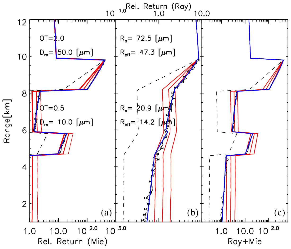
Figure B4Panels (a) to (c) show total simulated total attenuated backscatter, Rayleigh attenuated backscatter profile, and the total simulated attenuated backscatter profile (difference scale than the first columns) corresponding to a two-layer ice cloud system with the given layer parameters. The black lines (with the error bars) are the product of lidar Monte Carlo radiative transfer calculations. The dotted black lines are the single-scatter return values. The red lines are the results of Platt's approach using three different values of η (0.4,0.5,0.6). The blue lines show the result of applying Eq. (B5) together with Eq. (B8) using optimally chosen values of η and θSc for each of the two layers.
It should be noted that in this work η has been treated as being constant within a layer. Indeed, ηp is often employed as being constant in practical situations (e.g., Garnier et al., 2015); however, according to Platt (1981), ηp is treated as function of penetration depth and optical thickness. Our results indicate that by allowing for tails η can usefully be treated as being constant for a layer since the use of fe(z) gives the system the necessary degree of freedom. In a heuristic sense, using a constant η and a range-dependent fe(z) is somewhat equivalent to making η(z) range dependent.
The approach developed here, when applied to retrievals, is 𝒪(N2) efficient (due to the need to evaluate Eq. B8), while the approach described in Hogan and Battaglia (2008) is 𝒪(N) efficient. The approach described here has a lower baseline computational cost. Thus, roughly speaking, for a typical case where the resolution is on the order for 100 m, the two approaches have similar computational costs; however, for higher resolutions Hogans's PVC method becomes increasingly superior in this regard.
B4 MS extinction and backscatter corrections
Using a forward-modeling approach based on Eq. (B8), multiple-scattering effects, including the effects of tails, can be accounted for. For local methods employed to estimate the extinction, such as the approaches described in Appendix A, other correction type approaches are useful. In the following two sections the methods used to correct for multiple-scattering effects are described.
B4.1 Extinction
First, focusing on the extinction, starting with Eq. (B11) we can write
where
Taking the log of Eq. (B14) then yields
and then taking the derivative with range leads to
Now, if we define the effective extinction (i.e., the extinction that would be estimated assuming that no multiple scattering was occurring) as
then
Equation (B19) can easily be solved iteratively as follows.
-
The η and effective area radii (Ra) profiles must first be specified.
-
The f(z) profile (and its derivative) is calculated by using Eq. (B8).
-
The effective extinction is calculated using Eq. (B18).
-
τη is calculated using as a first guess for αM.
-
αM is updated using Eq. (B19).
-
τη is calculated using αM.
-
Steps (5) and (6) are repeated until convergence (typically two to three times).
In order to estimate the error, for simplicity it is assumed that the uncertainty in αM is dominated by the uncertainty in .
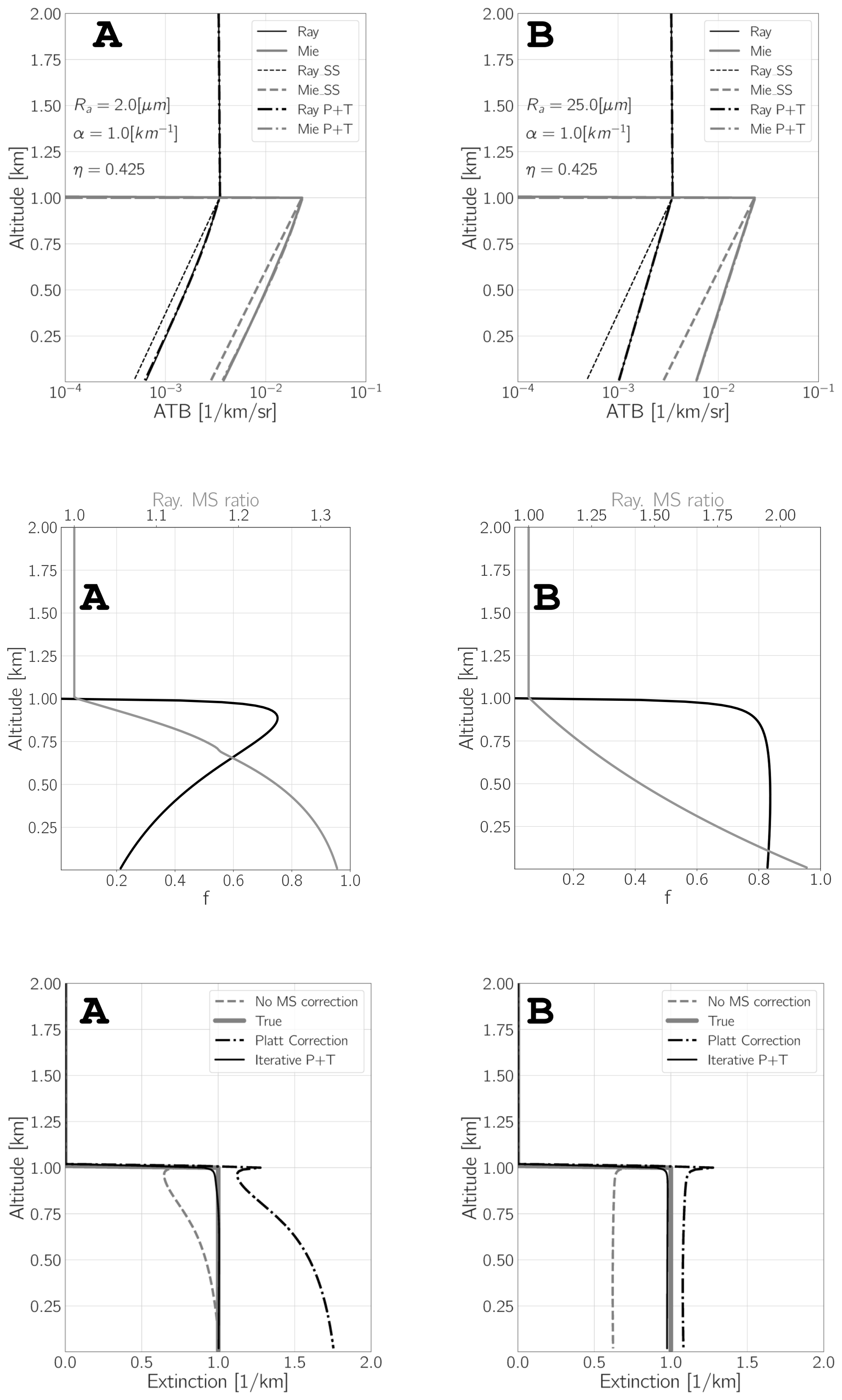
Figure B5Results of idealized simulations using homogeneous layers. The top panels show the Rayleigh and Mie attenuated backscatters assuming single-scattering data (“Ray_SS” and “Mie_SS”, respectively) and the profiles generated using the approach of Hogan (“Ray” and “Mie”, respectively) and the “P + T” approach with η=0.425. The middle panels show the f profiles generated using Eq. (B8) and the ratio between the Rayleigh ATBs including multiple-scattering data and the single-scattering ATBs. The bottom-left panels show the model truth extinction profile, the retrieved extinction profiles assuming no multiple-scattering effects, the extinction values that would be estimated using Platt's approach, and the results of iteratively applying Eq. (B19). The left column corresponds to the case where Ra = 2 [ µm], while the right column corresponds to the case where Ra = 25 [µm].
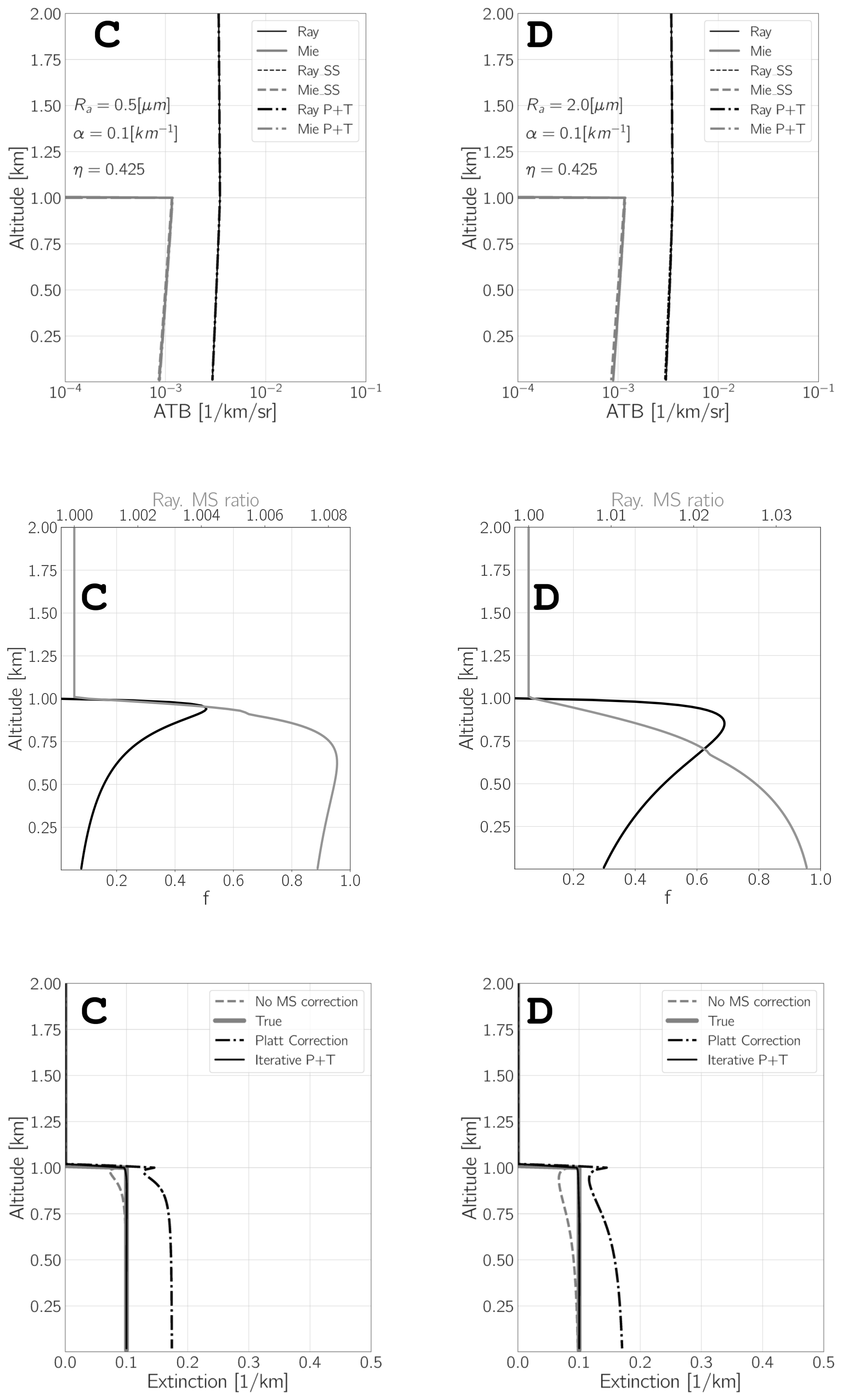
Figure B6The same as Fig. B5 but for an extinction coefficient of 0.1 km−1 and Ra = 0.5, and 2 µm, respectively.
The application of Eq. (B19) is illustrated by Figs. B5 and B6. Here four cases of homogeneous layers were considered covering a range of conditions from low extinction (αM = 0.1 km−1) to high extinction (αM = 1.0 km−1) and small and large particle sizes, respectively. A satellite altitude of 400 km was assumed, and the laser divergence and telescope FOV were set to 0.054 and 0.075 mrad (full angle), respectively.
Referring to Figs. B5 and B6, it can be seen in all the cases considered that the Platt + tails approach can provide a good match to the results generated by the approach of Hogan (Eq. B8) if η is set to a value of 0.425. It can also be seen that the extinction estimates made using Eq. (B19) are accurate to within under 10 % (here three iterations were used), whereas the estimates made when neglecting multiple scattering or using Platt's approach are subject to much larger errors in general.
B4.2 Backscatter
The observed (effective) backscatter can be related to the ratio of the Mie and Rayleigh attenuated backscatter using Eqs. (B11) and (B10) as follows:
When multiple scattering is not important (i.e., fe(z) = 0 or τη(z) = 0), then . However, when multiple scattering is important (i.e., fe(z) = 1 or 2τη(z)≫ 1), then . Once the extinction profile has been determined, as was described in the previous section, then the appropriate adjustment for multiple scattering can be calculated directly using Eq. (B20).
B4.3 Sensitivity
The accuracy of the procedures described in Sect. B4.1 and B4.2 is on the order of a few percent if the correct values of Ra, η, and fMSp are employed. However, this will not be the case in general. In order to assess the magnitude of the errors that may be expected due to the uncertainties in Ra, η, and fMSp, the simple simulated cases shown in Figs. B5 and B6 were inverted and corrected for multiple-scattering effects using Eq. (B19) and but using values of Ra, η, and fMSp different from the model truth values.
Examples of the impact of the particle size are shown in Figs. B7, B8 and B9. Here it can be seen that halving the values of the effective area radius leads to an underestimation of the extinction by about 10 %–15 % near the layer top, while doubling the effective area radius leads to an overestimation of the same rough magnitude. The corresponding errors in the lidar ratio follow the same pattern with somewhat higher percentage values.
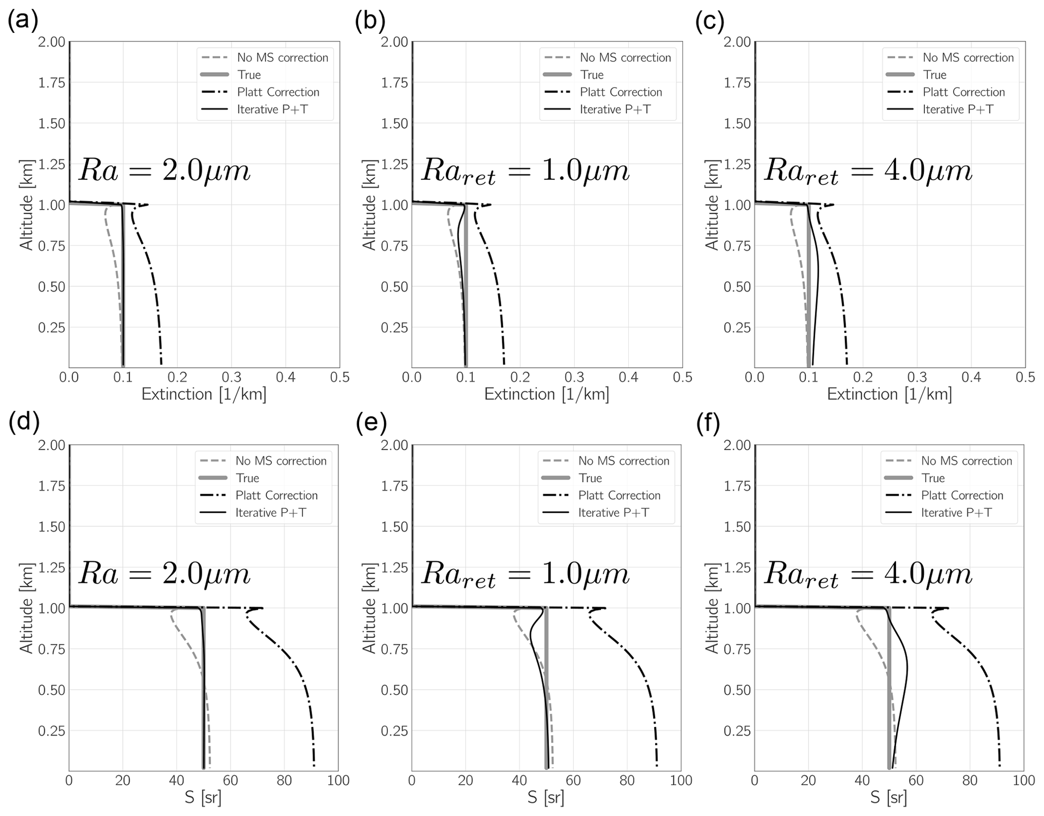
Figure B7(a, b, c) Extinction retrieved corresponding to case D in Fig. B6 using the indicated values of Ra. The corresponding retrieved lidar ratios are shown in panels (d), (e), and (f).
The relative errors resulting from errors in Ra do not depend strongly on the extinction itself; however, they can be strongly dependent on Ra. When Ra is of such a value that the associated θsc is much larger or smaller than ρt, then the impact of specifying Ra is limited. This is illustrated by Fig. B9, where it can be seen that halving the value of Ra used in the MS correction has a limited effect (less than 10 % at the layer bottom) on the estimated extinction and lidar ratio, while doubling the value of Ra used has practically no effect (since both 25 and 50 µm produce a small value of θsc compared to ρt).
The values of fMSp used for the MS correction procedure do not impact the retrieved extinction; however, the retrieved backscatter (and hence the estimated lidar ratio) will be impacted. In the limited case where f is close to 1, the relative errors in the retrieved backscatter (and associated lidar ratio) will directly correspond to the relative error in the value of fMSp used in the inversion.
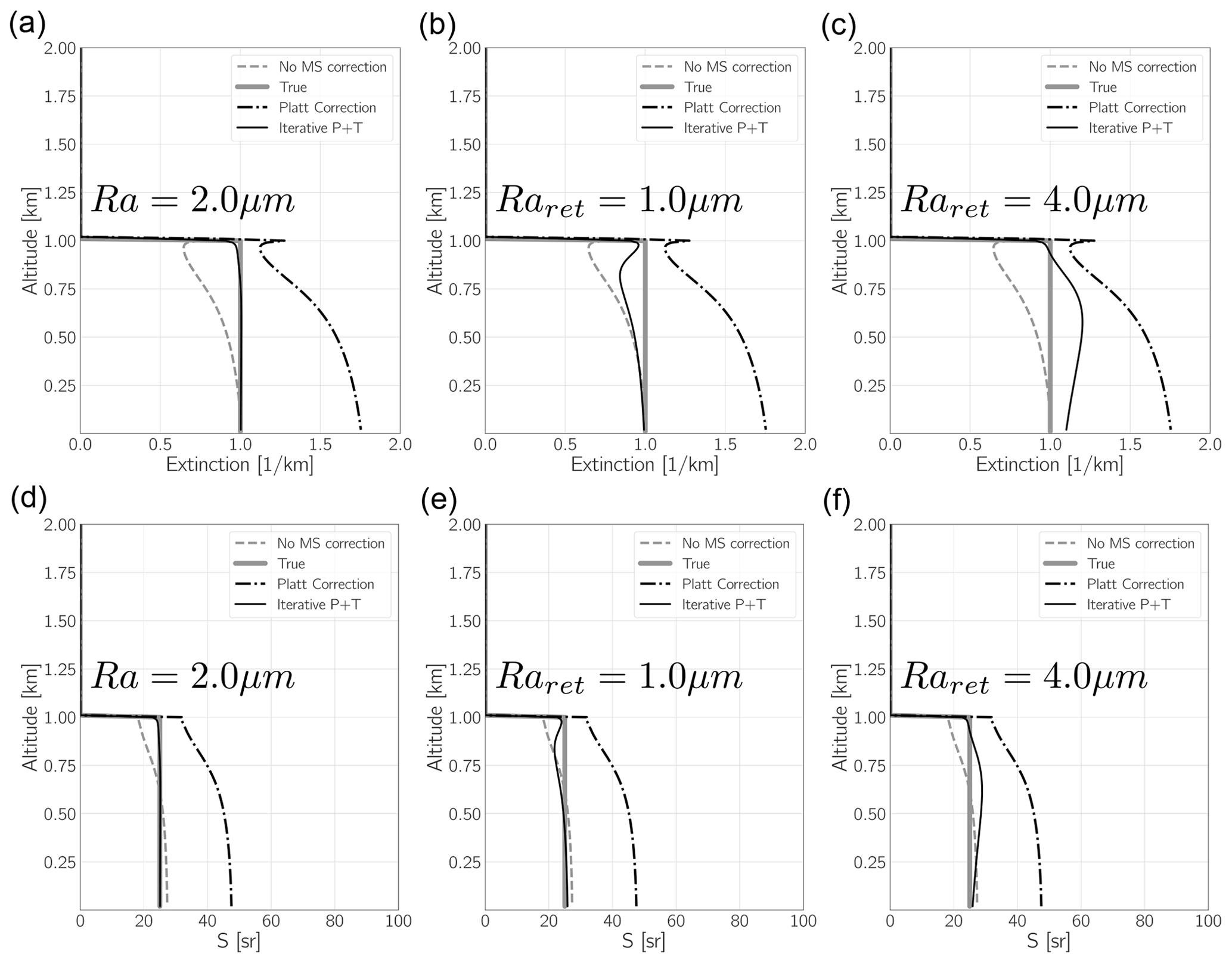
Figure B8(a, b, c) Extinction retrieved corresponding to case A in Fig. B6 using the indicated values of Ra. The corresponding retrieved lidar ratios are shown in panels (d), (e), and (f).
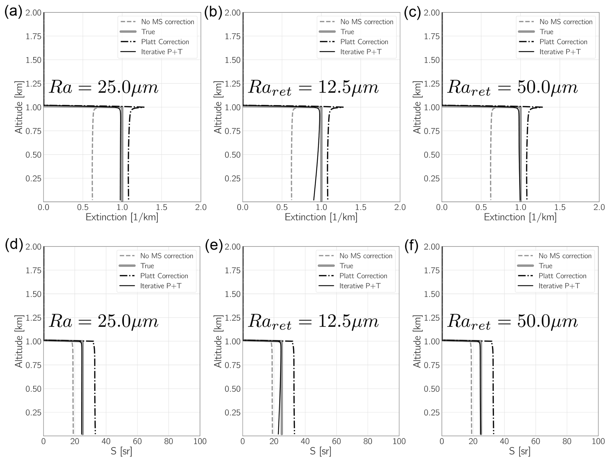
Figure B9(a, b, c) Extinction retrieved corresponding to case B in Fig. B6 using the indicated values of Ra. The corresponding retrieved lidar ratios are shown in panels (d), (e), and (f).
The sensitivity of the corrections to the assumed value of η were also investigated using trial values of 0.4 and 0.45. In all of the cases the impact was below 10 % for both the extinction and lidar ratio.
In summary, within layers, if the particle sizes care accurate within a factor of 2, maximum errors in the extinction and lidar ratio on the order of 10 %–15 % may be expected. The uncertainty in fMSp likely adds another 10 %–15 % to the uncertainty in the lidar ratio determination. For spherical scatterers, fMSp can be calculated using exact phase functions calculated using Mie theory (Hogan and Battaglia, 2008; Eloranta, 1998). For ice clouds, there is evidence for the general existence of a more pronounced backscatter peak (which implies values of fMSp significantly less than 1) even for irregular crystals (Zhou and Yang, 2015).
The above conclusions are relevant for single-layer situations. In the case of, for example, semi-transparent cirrus above aerosols, the sensitivity to the particle size especially can be more significant. This aspect is discussed in Sect. 3, where specific cases drawn from the GEM-ECSIM test scenes are discussed.
The explicit form of the forward model used by the A-EBD optimal-estimation retrieval and its Jacobian are presented here. Here i is used to denote the index of the forward-model element, and nz is the total number of range gates. Recall that the observation vector, and thus the forward-model vector, consists of the appended Rayleigh and Mie attenuated backscatters so that the length of the forward-model vector is 2nz.
For i≤nz we have, based on a discrete form of Eq. (B11),
where
and fe is the discrete version of Eq. (B9).
For i>nz we have, based on a discrete form of Eq. (B10),
Assuming for each range bin that the Mie and Rayleigh extinctions, lidar ratio, and f terms can be treated as being constant, evaluating the integral in Eq. (C1) then yields the following equation for the Rayleigh forward model:
It yields the following equation for the Mie forward model:
where
and
C1 Gradient and Jacobian elements
In order to efficiently minimize the cost function, we must be able to compute its gradient with respect to the elements of the state vector. The gradient of the cost function is related to the Jacobian of the forward model as follows:
where JF is the forward-model Jacobian with respect to the state variables, i.e.,
where refers to the linear counterpart of the element of the log state vector element xj, i.e., .
C1.1 Derivatives with respect to extinction
Using the forward model the partial derivatives with respect to the particulate extinctions are as follows.
For we use the following equation:
For we use the following equation:
where
and
For we use the following equation:
For we use the following equation:
Derivatives with respect to lidar ratio
For the lidar ratio elements of the state vector, one must take into account that the state vector elements represent extended layers. Thus,
where and i≤nz. Here jt,j is the range index of the layer top for the layer corresponding to the lth element of the state vector, while jb,j is the range index of the layer bottom for the layer corresponding to the lth element of the state vector.
For we use the following equation:
For j<i we use the following equation:
For i=j we use the following equation:
C2 Derivatives with respect to particle size
For the Ra elements of the state vector, as is the case for the lidar ratio, one must take into account that the state vector elements represent extended layers. Thus,
where m i≤nz, and
For j≤i we use the following equation:
where
For we use the following equation:
For j≤nz we use the following equation:
Derivatives with respect to Clid
For and i≤nz we use the following equation:
For we use the following equation:
The EarthCARE level-2 (L2) nadir model truth data and the simulated L2 products discussed in this paper are available from https://doi.org/10.5281/zenodo.7117115 (van Zadelhoff et al., 2023a).
The lead author of this paper (DPD) was also the lead developer of the A-PRO processor. GJvZ contributed to the writing of the code and was the lead developer of the A-TC components. PW assisted in the evaluation and testing of the code. All authors contributed to the writing and editing of the manuscript.
The contact author has declared that none of the authors has any competing interests.
Publisher’s note: Copernicus Publications remains neutral with regard to jurisdictional claims made in the text, published maps, institutional affiliations, or any other geographical representation in this paper. While Copernicus Publications makes every effort to include appropriate place names, the final responsibility lies with the authors.
This article is part of the special issue “EarthCARE Level 2 algorithms and data products”. It is not associated with a conference.
We thank Tobias Wehr, Michael Eisinger, and Anthony Illingworth for valuable discussions and their support for this work over many years. A special acknowledgement is in order for Tobias Wehr, ESA's EarthCARE Mission Scientist, who unexpectedly passed away recently. Tobias was eagerly looking forward to EarthCARE's launch, a mission to which he had dedicated a considerable span of his career. His support for the science community, collaborative approach, and enthusiasm for the mission science will not be forgotten.
This research has been supported by the European Space Agency (ESA) grant nos. 22638/09/NL/CT (ATLAS), ITT 1-7879/14/NL/CT (APRIL), and 4000134661/21/NL/AD (CARDINAL)).
This paper was edited by Edward Nowottnick and reviewed by two anonymous referees.
Dai, G., Wu, S., Long, W., Liu, J., Xie, Y., Sun, K., Meng, F., Song, X., Huang, Z., and Chen, W.: Aerosol and cloud data processing and optical property retrieval algorithms for the spaceborne ACDL/DQ-1, Atmos. Meas. Tech., 17, 1879–1890, https://doi.org/10.5194/amt-17-1879-2024, 2024. a
do Carmo, J. P., Hélière, A., Le Hors, L., Toulemont, Y., Lefebvre, A., and Lefebvre, A.: ATLID, ESA Atmospheric LIDAR Developement Status, EPJ Web Conf., 119, 04003, https://doi.org/10.1051/epjconf/201611904003, 2016. a
do Carmo, J. P., de Villele, G., Wallace, K., Lefebvre, A., Ghose, K., Kanitz, T., Chassat, F., Corselle, B., Belhadj, T., and Bravetti, P.: ATmospheric LIDar (ATLID): Pre-Launch Testing and Calibration of the European Space Agency Instrument That Will Measure Aerosols and Thin Clouds in the Atmosphere, Atmosphere, 12, 76, https://doi.org/10.3390/atmos12010076, 2021. a, b
Dong, J., Liu, J., Bi, D., Ma, X., Zhu, X., Zhu, X., and Chen, W.: Optimal iodine absorption line applied for spaceborne high spectral resolution lidar, Appl. Optics, 57, 5413–5419, https://doi.org/10.1364/AO.57.005413, 2018. a
Donovan, D. P., Klein Baltink, H., Henzing, J. S., de Roode, S. R., and Siebesma, A. P.: A depolarisation lidar-based method for the determination of liquid-cloud microphysical properties, Atmos. Meas. Tech., 8, 237–266, https://doi.org/10.5194/amt-8-237-2015, 2015. a
Donovan, D. P., Kollias, P., Velázquez Blázquez, A., and van Zadelhoff, G.-J.: The generation of EarthCARE L1 test data sets using atmospheric model data sets, Atmos. Meas. Tech., 16, 5327–5356, https://doi.org/10.5194/amt-16-5327-2023, 2023. a, b, c, d
Ehlers, F., Flament, T., Dabas, A., Trapon, D., Lacour, A., Baars, H., and Straume-Lindner, A. G.: Optimization of Aeolus' aerosol optical properties by maximum-likelihood estimation, Atmos. Meas. Tech., 15, 185–203, https://doi.org/10.5194/amt-15-185-2022, 2022. a
Eisinger, M., Wehr, T., Kubota, T., Bernaerts, D., and Wallace, K.: The EarthCARE production model and auxiliary products, Atmos. Meas. Tech., in preparation, 2022. a, b, c
Eisinger, M., Marnas, F., Wallace, K., Kubota, T., Tomiyama, N., Ohno, Y., Tanaka, T., Tomita, E., Wehr, T., and Bernaerts, D.: The EarthCARE mission: science data processing chain overview, Atmos. Meas. Tech., 17, 839–862, https://doi.org/10.5194/amt-17-839-2024, 2024. a, b
Eloranta, E.: Lidar: Range-Resolved Optical Remote Sensing of the Atmosphere, High Spectral Resolution Lidar, edited by: Weitkamp, C., Springer, Berlin, 143–163, https://doi.org/10.1007/b106786 2005. a, b, c, d
Eloranta, E. W.: Practical model for the calculation of multiply scattered lidar returns, Appl. Optics, 37, 2464–2472, https://doi.org/10.1364/AO.37.002464, 1998. a, b
Flament, T., Trapon, D., Lacour, A., Dabas, A., Ehlers, F., and Huber, D.: Aeolus L2A aerosol optical properties product: standard correct algorithm and Mie correct algorithm, Atmos. Meas. Tech., 14, 7851–7871, https://doi.org/10.5194/amt-14-7851-2021, 2021. a
Garnier, A., Pelon, J., Vaughan, M. A., Winker, D. M., Trepte, C. R., and Dubuisson, P.: Lidar multiple scattering factors inferred from CALIPSO lidar and IIR retrievals of semi-transparent cirrus cloud optical depths over oceans, Atmos. Meas. Tech., 8, 2759–2774, https://doi.org/10.5194/amt-8-2759-2015, 2015. a
Heymsfield, A., Winker, D., Avery, M., Vaughan, M., Diskin, G., Deng, M., Mitev, V., and Matthey, R.: Relationships between Ice Water Content and Volume Extinction Coefficient from In Situ Observations for Temperatures from 0 ° to −86 °C: Implications for Spaceborne Lidar Retrievals, J. Appl. Meteorol. Clim., 53, 479–505, https://doi.org/10.1175/JAMC-D-13-087.1, 2014. a, b
Heymsfield, A. J., Winker, D., and van Zadelhoff, G.-J.: Extinction-ice water content-effective radius algorithms for CALIPSO, Geophys. Res. Lett., 32, L10807, https://doi.org/10.1029/2005GL022742, 2005. a
Hogan, R. J.: Fast approximate calculation of multiply scattered lidar returns, Appl. Optics, 45, 5984–5992, https://doi.org/10.1364/AO.45.005984, 2006. a
Hogan, R. J.: Fast Lidar and Radar Multiple-Scattering Models. Part I: Small-Angle Scattering Using the Photon Variance–Covariance Method, J. Atmos. Sci., 65, 3621–3635, https://doi.org/10.1175/2008JAS2642.1, 2008. a, b, c, d
Hogan, R. J. and Battaglia, A.: Fast Lidar and Radar Multiple-Scattering Models. Part II: Wide-Angle Scattering Using the Time-Dependent Two-Stream Approximation, J. Atmos. Sci., 65, 3636–3651, https://doi.org/10.1175/2008JAS2643.1, 2008. a, b, c, d
Hu, Y., Winker, D., Vaughan, M., Lin, B., Omar, A., Trepte, C., Flittner, D., Yang, P., Nasiri, S. L., Baum, B., Holz, R., Sun, W., Liu, Z., Wang, Z., Young, S., Stamnes, K., Huang, J., and Kuehn, R.: CALIPSO/CALIOP Cloud Phase Discrimination Algorithm, J. Atmos. Ocean. Tech., 26, 2293–2309, https://doi.org/10.1175/2009JTECHA1280.1, 2009. a
Illingworth, A. J., Barker, H. W., Beljaars, A., Ceccaldi, M., Chepfer, H., Clerbaux, N., Cole, J., Delanoë, J., Domenech, C., Donovan, D. P., Fukuda, S., Hirakata, M., Hogan, R. J., Huenerbein, A., Kollias, P., Kubota, T., Nakajima, T., Nakajima, T. Y., Nishizawa, T., Ohno, Y., Okamoto, H., Oki, R., Sato, K., Satoh, M., Shephard, M. W., Velázquez-Blázquez, A., Wandinger, U., Wehr, T., and van Zadelhoff, G.-J.: The EarthCARE Satellite: The Next Step Forward in Global Measurements of Clouds, Aerosols, Precipitation, and Radiation, B. Am. Meteorol. Soc., 96, 1311–1332, https://doi.org/10.1175/BAMS-D-12-00227.1, 2015. a
Irbah, A., Delanoë, J., van Zadelhoff, G.-J., Donovan, D. P., Kollias, P., Puigdomènech Treserras, B., Mason, S., Hogan, R. J., and Tatarevic, A.: The classification of atmospheric hydrometeors and aerosols from the EarthCARE radar and lidar: the A-TC, C-TC and AC-TC products, Atmos. Meas. Tech., 16, 2795–2820, https://doi.org/10.5194/amt-16-2795-2023, 2023. a, b, c, d, e, f
Kliewer, A. J., Fletcher, S. J., Jones, A. S., and Forsythe, J. M.: Comparison of Gaussian, logarithmic transform and mixed Gaussian–log-normal distribution based 1DVAR microwave temperature–water-vapour mixing ratio retrievals, Q. J. Roy. Meteor. Soc., 142, 274–286, https://doi.org/10.1002/qj.2651, 2016. a, b
Liu, Q., Huang, Z., Liu, J., Chen, W., Dong, Q., Wu, S., Dai, G., Li, M., Li, W., Li, Z., Song, X., and Xie, Y.: Validation of initial observation from the first spaceborne high-spectral-resolution lidar with a ground-based lidar network, Atmos. Meas. Tech., 17, 1403–1417, https://doi.org/10.5194/amt-17-1403-2024, 2024. a
Maahn, M., Turner, D. D., Löhnert, U., Posselt, D. J., Ebell, K., Mace, G. G., and Comstock, J. M.: Optimal Estimation Retrievals and Their Uncertainties: What Every Atmospheric Scientist Should Know, B. Am. Meteorol. Soc., 101, E1512–E1523, https://doi.org/10.1175/BAMS-D-19-0027.1, 2020. a
Mason, S. L., Cole, J. N. S., Docter, N., Donovan, D. P., Hogan, R. J., Hünerbein, A., Kollias, P., Puigdomènech Treserras, B., Qu, Z., Wandinger, U., and van Zadelhoff, G.-J.: An intercomparison of EarthCARE cloud, aerosol and precipitation retrieval products, EGUsphere [preprint], https://doi.org/10.5194/egusphere-2023-1682, 2023a. a, b
Mason, S. L., Hogan, R. J., Bozzo, A., and Pounder, N. L.: A unified synergistic retrieval of clouds, aerosols, and precipitation from EarthCARE: the ACM-CAP product, Atmos. Meas. Tech., 16, 3459–3486, https://doi.org/10.5194/amt-16-3459-2023, 2023b. a
Platt, C. M. R.: Infrared absorption and liquid water content in stratocumulus clouds, Q. J. Roy. Meteor. Soc., 102, 553–561, https://doi.org/10.1002/qj.49710243305, 1976. a
Platt, C. M. R.: Remote Sounding of High Clouds. III: Monte Carlo Calculations of Multiple-Scattered Lidar Returns, J. Atmos. Sci., 38, 156–167, https://doi.org/10.1175/1520-0469(1981)038<0156:RSOHCI>2.0.CO;2, 1981. a, b, c
Press, W. H., Teukolsky, S. A., Vetterling, W. T., and Flannery, B. P.: Numerical Recipes 3rd Edition: The Art of Scientific Computing, Cambridge University Press, 3rd edn., ISBN 0521880688, https://www.amazon.com/Numerical-Recipes-3rd-Scientific-Computing/dp/0521880688/ref=sr_1_1?ie=UTF8&s=books&qid=1280322496&sr=8-1 (last access: 28 August 2024), 2007. a, b
Qu, Z., Donovan, D. P., Barker, H. W., Cole, J. N. S., Shephard, M. W., and Huijnen, V.: Numerical model generation of test frames for pre-launch studies of EarthCARE's retrieval algorithms and data management system, Atmos. Meas. Tech., 16, 4927–4946, https://doi.org/10.5194/amt-16-4927-2023, 2023. a
Russ, J. C.: The Image Processing Handbook, 5th edn., CRC Press, ISBN 9780849372544, 2007. a
Straume, A. G., Rennie, M., Isaksen, L., de Kloe, J., Marseille, G.-J., Stoffelen, A., Flament, T., Stieglitz, H., Dabas, A., Huber, D., Reitebuch, O., Lemmerz, C., Lux, O., Marksteiner, U., Weiler, F., Witschas, B., Meringer, M., Schmidt, K., Nikolaus, I., Geiss, A., Flamant, P., Kanitz, T., Wernham, D., von Bismarck, J., Bley, S., Fehr, T., Floberghagen, R., and Parinello, T.: ESA’s Space-Based Doppler Wind Lidar Mission Aeolus – First Wind and Aerosol Product Assessment Results, EPJ Web Conf., 237, 01007, https://doi.org/10.1051/epjconf/202023701007, 2020. a, b
van Zadelhoff, G.-J., Barker, H. W., Baudrez, E., Bley, S., Clerbaux, N., Cole, J. N. S., de Kloe, J., Docter, N., Domenech, C., Donovan, D. P., Dufresne, J.-L., Eisinger, M., Fischer, J., García-Marañón, R., Haarig, M., Hogan, R. J., Hünerbein, A., Kollias, P., Koopman, R., Madenach, N., Mason, S. L., Preusker, R., Puigdomènech Treserras, B., Qu, Z., Ruiz-Saldaña, M., Shephard, M., Velázquez-Blazquez, A., Villefranque, N., Wandinger, U., Wang, P., and Wehr, T.: EarthCARE level-2 demonstration products from simulated scenes, Zenodo [data set], https://doi.org/10.5281/zenodo.7117115, 2023a. a
van Zadelhoff, G.-J., Donovan, D. P., and Wang, P.: Detection of aerosol and cloud features for the EarthCARE atmospheric lidar (ATLID): the ATLID FeatureMask (A-FM) product, Atmos. Meas. Tech., 16, 3631–3651, https://doi.org/10.5194/amt-16-3631-2023, 2023b. a, b, c, d
Vaughan, M. A., Powell, K. A., Winker, D. M., Hostetler, C. A., Kuehn, R. E., Hunt, W. H., Getzewich, B. J., Young, S. A., Liu, Z., and McGill, M. J.: Fully Automated Detection of Cloud and Aerosol Layers in the CALIPSO Lidar Measurements, J. Atmos. Ocean. Tech., 26, 2034–2050, https://doi.org/10.1175/2009JTECHA1228.1, 2009. a
Wandinger, U.: Multiple-scattering influence on extinction- and backscatter-coefficient measurements with Raman and high-spectral-resolution lidars, Appl. Optics, 37, 417–427, https://doi.org/10.1364/AO.37.000417, 1998. a
Wandinger, U., Floutsi, A. A., Baars, H., Haarig, M., Ansmann, A., Hünerbein, A., Docter, N., Donovan, D., van Zadelhoff, G.-J., Mason, S., and Cole, J.: HETEAC – the Hybrid End-To-End Aerosol Classification model for EarthCARE, Atmos. Meas. Tech., 16, 2485–2510, https://doi.org/10.5194/amt-16-2485-2023, 2023. a
Wang, P., Donovan, D. P., van Zadelhoff, G.-J., de Kloe, J., Huber, D., and Reissig, K.: Evaluation of Aeolus feature mask and particle extinction coefficient profile products using CALIPSO data, EGUsphere [preprint], https://doi.org/10.5194/egusphere-2024-731, 2024. a, b
Wang, W., Gong, W., Mao, F., Pan, Z., and Liu, B.: Measurement and Study of Lidar Ratio by Using a Raman Lidar in Central China, Int. J. Env. Res. Pub. He., 13, 508, https://doi.org/10.3390/ijerph13050508, 2016. a
Wehr, T., Kubota, T., Tzeremes, G., Wallace, K., Nakatsuka, H., Ohno, Y., Koopman, R., Rusli, S., Kikuchi, M., Eisinger, M., Tanaka, T., Taga, M., Deghaye, P., Tomita, E., and Bernaerts, D.: The EarthCARE mission – science and system overview, Atmos. Meas. Tech., 16, 3581–3608, https://doi.org/10.5194/amt-16-3581-2023, 2023. a
Winker, D.: Accounting for multiple scattering in retrievals from space lidar, SPIE, 5059, https://doi.org/10.1117/12.512352, 2003. a
Zhou, C. and Yang, P.: Backscattering peak of ice cloud particles, Opt. Express, 23, 11995–12003, https://doi.org/10.1364/OE.23.011995, 2015. a, b
- Abstract
- Introduction
- A-PRO retrieval processor
- Case studies using simulated data
- Conclusion and outlook
- Appendix A: A-AER extinction, backscatter, and lidar ratio retrieval methods
- Appendix B: Treatment of multiple scattering for ATLID in A-PRO
- Appendix C: A-EBD forward model and Jacobian
- Data availability
- Author contributions
- Competing interests
- Disclaimer
- Special issue statement
- Acknowledgements
- Financial support
- Review statement
- References