the Creative Commons Attribution 4.0 License.
the Creative Commons Attribution 4.0 License.
 | 16 Sep 2024
Methane retrieval from MethaneAIR using the CO2 proxy approach: a demonstration for the upcoming MethaneSAT mission
Christopher Chan Miller
Sébastien Roche
Jonas S. Wilzewski
Xiong Liu
Kelly Chance
Amir H. Souri
Eamon Conway
Bingkun Luo
Jenna Samra
Jacob Hawthorne
Carly Staebell
Apisada Chulakadabba
Maryann Sargent
Joshua S. Benmergui
Jonathan E. Franklin
Bruce C. Daube
Joshua L. Laughner
Bianca C. Baier
Ritesh Gautam
Mark Omara
Steven C. Wofsy
Reducing methane (CH4) emissions from the oil and gas (O&G) sector is crucial for mitigating climate change in the near term. MethaneSAT is an upcoming satellite mission designed to monitor basin-wide O&G emissions globally, providing estimates of emission rates and helping identify the underlying processes leading to methane release in the atmosphere. MethaneSAT data will support advocacy and policy efforts by helping to track methane reduction commitments and targets set by countries and industries. Here, we introduce a CH4 retrieval algorithm for MethaneSAT based on the CO2 proxy method. We apply the algorithm to observations from the maiden campaign of MethaneAIR, an airborne precursor to the satellite that has similar instrument specifications. The campaign was conducted during winter 2019 and summer 2021 over three major US oil and gas basins.
Analysis of MethaneAIR data shows that measurement precision is typically better than 2 % at a 20×20 m2 pixel resolution, exhibiting no strong dependence on geophysical variables, e.g., surface reflectance. We show that detector focus drifts over the course of each flight, likely due to thermal gradients that develop across the optical bench. The impacts of this drift on retrieved CH4 can mostly be mitigated by including a parameter that squeezes the laboratory-derived, tabulated instrument spectral response function (ISRF) in the spectral fit. Validation against coincident EM27/SUN retrievals shows that MethaneAIR values are generally within 1 % of the retrievals. MethaneAIR retrievals were also intercompared with retrievals from the TROPOspheric Monitoring Instrument (TROPOMI). We estimate that the mean bias between the instruments is 2.5 ppb, and the latitudinal gradients for the two data sets are in good agreement.
We evaluate the accuracy of MethaneAIR estimates of point-source emissions using observations recorded over the Permian Basin, an O&G basin, based on the integrated-mass-enhancement approach coupled with a plume-masking algorithm that uses total variational denoising. We estimate that the median point-source detection threshold is 100–150 kg h−1 at the aircraft's nominal above-surface observation altitude of 12 km. This estimate is based on an ensemble of Weather Research and Forecasting (WRF) large-eddy simulations used to mimic the campaign's conditions, with the threshold for quantification set at approximately twice the detection threshold. Retrievals from repeated basin surveys indicate the presence of both persistent and intermittent sources, and we highlight an example from each case. For the persistent source, we infer emissions from a large O&G processing facility and estimate a leak rate between 1.6 % and 2.1 %, higher than any previously reported emission levels from a facility of its size. We also identify a ruptured pipeline that could increase total basin emissions by 2 % if left unrepaired; this pipeline was discovered 2 weeks before it was found by its operator, highlighting the importance of regular monitoring by future satellite missions. The results showcase MethaneAIR's capability to make highly accurate, precise measurements of methane dry-air mole fractions in the atmosphere, with a fine spatial resolution (∼ 20×20 m2) mapped over large swaths (∼ 100×100 km2) in a single flight. The results provide confidence that MethaneSAT can make such measurements at unprecedentedly fine scales from space (∼ 130×400 m2 pixel size over a target area measuring ∼ 200×200 km2), thereby delivering quantitative data on basin-wide methane emissions.
- Article
(21259 KB) - Full-text XML
-
Supplement
(3833 KB) - BibTeX
- EndNote


Methane (CH4) is the second most important human-influenced greenhouse gas (GHG), with a radiative forcing corresponding to one-third of the magnitude of carbon dioxide (CO2) (Etminan et al., 2016). Recently, there has been considerable policy focus on reducing anthropogenic methane emissions, underscored by over 100 nations agreeing at the COP26 meeting in Glasgow in 2021 to a 30 % reduction from 2020 levels by 2030 (Malley et al., 2023). These reductions are expected to be driven largely by tightened emission controls on the O&G sector (White House Climate Policy Office, 2021), due mainly to their cost-effectiveness relative to other major anthropogenic sources (UNEP, 2021). Improved monitoring is required to help companies and regulators understand where and why methane emissions occur, to quantify emission rates in large O&G production regions, and to ensure that both nations and major O&G producers meet their stated commitments.
MethaneSAT, launched in March 2024, is a satellite mission designed with the primary goal of quantifying all CH4 emissions from major O&G production basins at a high spatial resolution with regular revisits. It is funded by private philanthropy and is managed by MethaneSAT LLC, a wholly owned subsidiary of the Environmental Defense Fund. In preparation for MethaneSAT's launch, an airborne precursor called MethaneAIR was constructed (Staebell et al., 2021), with near-identical instrument specifications (Table S1 in the Supplement; Chulakadaba et al., 2023). Here, we use MethaneAIR observations from its maiden flight campaign to validate the MethaneSAT CO2-proxy-based CH4 algorithm used to retrieve dry-air column-averaged CH4 mole fractions (XCH4) and report on the accuracy of emission rate determinations using this sensor.
Remote-sensed CH4 observations are the most efficient way to map methane emissions at a large scale. Satellites have been monitoring CH4 globally since the launch of the SCanning Imaging Absorption spectroMeter for Atmospheric CartograpHY (SCIAMACHY) in 2002 (Frankenberg et al., 2006). The TROPOspheric Monitoring Instrument (TROPOMI), the most recent of this class of global CH4 mappers, was launched in 2017. It has a 5.5×7 km2 spatial resolution with daily global coverage, producing observations with pixels ∼ 90× smaller than SCIAMACHY pixels and covering the globe 6× faster (Hu et al., 2018). This class of sensors, particularly Greenhouse Gases Observing Satellite (GOSAT) sensors (Parker et al., 2020), has been used to regionally constrain methane emissions (Monteil et al., 2013; Turner et al., 2015; Maasakkers et al., 2019; Lu et al., 2021; Zhang et al., 2021; Qu et al., 2022), proving useful for identifying drivers of global CH4 trends (Deng et al., 2022; Janardanan et al., 2020; Worden et al., 2022). Currently, TROPOMI is used less in global inversions due to region-specific retrieval biases (Qu et al., 2021; Jacob et al., 2022); however, its high spatiotemporal coverage makes it the first global mapper capable of constraining total O&G basin CH4 emissions, and its retrievals have been used to reveal large emission underestimates for multiple basins (Schneising et al., 2020; Zhang et al., 2020; Shen et al., 2021, 2022). Nevertheless, reliable basin-wide emission estimates require months of TROPOMI data due to the low 3 % retrieval success rate, a result of unfavorable scene conditions (reflectance, cloud, and aerosols), and the limited robustness of the full-physics approach (Jacob et al., 2022). The CO2 proxy approach has proven more robust under moderate aerosol conditions (Parker et al., 2015), with the GOSAT CO2 proxy retrieval showing a 24 % success rate (Parker et al., 2020). Here, aerosol scattering is implicitly accounted for by normalizing the retrieved CH4 column against a CO2 column retrieved from the same spectral region. The CO2 proxy approach is not possible with TROPOMI as there is no nearby CO2 absorption in the targeted 2.3 µm CH4 band.
Recently, instruments designed to detect high concentrations of CH4 in individual methane plumes have been deployed on aircraft (e.g., the Airborne Visible/Infrared Imaging Spectrometer (AVIRIS; Thorpe et al., 2012), AVIRIS – Next Generation (AVIRIS–NG; Thorpe et al., 2016), and HySpex (Hochstaffl et al., 2023)) and satellites (Sentinel-2 (Varon et al., 2021), GHGSat (Jervis et al., 2021), Carbon Mapper (Shivers et al., 2021), PRISMA (Guanter et al., 2021), and EnMAP (Roger et al., 2024)) to estimate emission rates from point sources. Such instruments have an increased pixel resolution (∼ 1–10 m length scale) at the expense of the spectral resolution (∼ 10 nm vs. ∼ 0.1 nm for global mappers). At these spatial scales, CH4 concentrations from plumes originating from point sources can be much higher than the atmospheric background, loosening the retrieval accuracy requirement. They have proven particularly useful for monitoring emissions from O&G infrastructure, where emissions from individual facilities follow heavy-tailed distributions (Brandt et al., 2016; Zavala-Araiza et al., 2015; Frankenberg et al., 2016; Cusworth et al., 2021). However, it is not possible to determine how many emissions within a basin are measured by observing a small number of detectable superemitters, and such measurements can miss a substantial proportion of emissions from smaller sources.
In fact, recent work has suggested that these smaller sources represent a significant fraction of total O&G methane emissions. From a statistical survey of observed site-level O&G well emissions, Omara et al. (2022) estimated that low-production wells account for over 50 % of all US O&G-production-related methane emissions due to their high production-normalized leak rates (>10 % on average) and prevalence (81 % of all producing wells). However, because emissions from individual low-producing wells are low (95 % of sites emit less than 7 kg h−1), they are invisible to current and future satellite instruments used to detect methane point sources as these instruments have detection limits that are at least an order of magnitude larger1. Aircraft sensors, such as AVIRIS-NG, have plume detection limits as low as 10 kg h−1 (Thorpe et al., 2016), enabling the detection of the highest-emitting low-production wells. However, these reported detection limits correspond to ground pixel sizes of ∼ 0.5 m, meaning observations need to be made close to the surface (0.5–1 km). Mapping a basin in such a manner would require many days of flying. Recently, Cusworth et al. (2022) conducted a large survey of US O&G basins using the AVIRIS-NG instrument, flying at altitudes more suitable for large-scale surveying (3–5 km). By comparing their data with basin emissions inferred from TROPOMI, they estimated that they were able to constrain about 35 % of total emissions from oil and gas infrastructure, leaving about two-thirds of basin emissions unmeasured. The ability of these sensors to assign sources to specific infrastructure provides insights into the specific practices and activities contributing to the basin's total emissions from large point sources. However, a complete monitoring strategy requires this type of sensor to be used in combination with sensors capable of regularly measuring total basin emissions and the spatial distribution of diffuse emissions.
MethaneSAT has been designed to bridge the gap between space-borne global flux mappers and point-source imaging instruments. It contains a pair of 2D grating spectrometers with a spectral resolution similar to that of TROPOMI, covering the 1.27 µm O2 singlet delta () and 1.65 µm (2ν3) CH4 bands. Unlike TROPOMI and upcoming missions (such as CO2M; Sierk et al., 2019), which acquire broad swaths to achieve daily global coverage, MethaneSAT is maneuverable and designed to target scenes at approximately the scale of an O&G production basin (200×200 km2 at nadir for a 30 s collection time). By concentrating pixels on a smaller acquisition area, it achieves a pixel size of 130×400 m2 in its nominal operational mode, allowing CH4 to be retrieved with the accuracy of a TROPOMI-like instrument (Jacob et al., 2022) but with a spatial resolution capable of imaging individual plumes from point sources. This unique combination of a high spatial resolution, high measurement precision, and wide swath will enable both the estimation of point-source emissions from high-emitting facilities and the quantification and mapping of the entire basin source via the inversion of an emission field, representing the sum of sources below the plume detection threshold. MethaneSAT will acquire an average of 30 scenes per day, enabling at least 10–20 revisits to major O&G basins per year. Targets will be prioritized based on production rates of oil and gas and scheduled based on favorable meteorological forecast conditions (e.g., low cloud cover and steady winds) for both retrieval and emission inversion, maximizing the utility of each acquisition (Benmergui, 2019).
Here, we present results from the maiden flight campaign of MethaneAIR using the operational MethaneSAT CO2-proxy-based XCH4 retrieval. This is expected to be the primary XCH4 product used in subsequent emission inversions2. The CO2 proxy method was first used on an airborne platform by the Methane Airborne MAPper (MAMAP) instrument (Krings et al., 2011; Gerilowski et al., 2011), which provided the first remote-sensed estimates of point sources and small-area sources of both CH4 and CO2 (Krautwurst et al., 2017; Krings et al., 2018). MethaneAIR builds on this heritage by substantially increasing the sensor's spatial-coverage rate, mapping approximately 490 times the area per unit time relative to the MAMAP instrument. This is achieved through its higher nominal operating altitude (12 vs. 1.25 km), faster aircraft speed (720 vs. 200 km h−1), higher exposure time (0.1 vs. 0.6 s), and configuration as a push-broom scanner (983 across-track pixels vs. 1 across-track pixel). This allows for complete mapping of a typically sized oil and gas basin in just a few hours of flight time.
The road map for the rest of the paper is as follows. Section 2 describes the flight campaign, and Sect. 3 details the retrieval methodology. Section 4 describes the method used for retrieval bias correction, necessitated by drifts caused by the impact of cabin temperature changes during flights. The MethaneAIR observations are validated against ground-based (EM27/SUN) and satellite (TROPOMI) retrievals in Sect. 5. The results of this validation are used to estimate the MethaneAIR detection limit for point sources and further discuss challenges for the CH4 emission inversion problem at fine spatial scales based on the observations (Sect. 6). We highlight some case studies based on observations from the Permian Basin in Sect. 7. Lastly, in Sect. 8, we discuss the implications for MethaneSAT.
The first two MethaneAIR flights took place in November 2019 aboard the High-performance Instrumented Airborne Platform for Environmental Research (HIAPER) Gulfstream V (GV) aircraft from the National Science Foundation (NSF) and the National Center for Atmospheric Research (NCAR) (UCAR/NCAR – Earth Observing Laboratory, 2005). The remaining eight flights were conducted from July–August 2021; they were delayed initially by aircraft issues and later by the COVID-19 pandemic. Figure 1 shows the flight path for the first nine flights, during which the instrument was operating in nadir-viewing mode. For the final flight, the instrument orientation was switched to a zenith orientation to observe oxygen airglow in the early evening.
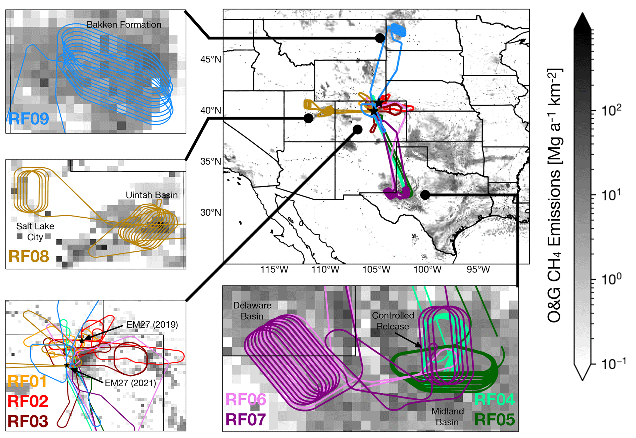
Figure 1Aircraft flight paths for the nine nadir-viewing research flights from the first campaign, overlaid on top of an illustration of total oil and gas emissions (Scarpelli et al., 2020). Black stars indicate the locations of the EM27/SUN spectrometers used for validation.
The first three research flights (RF01–RF03) were performed for engineering assessments and instrument functions. These flights were conducted around the Colorado Front Range region near the project base airport in Broomfield, Colorado, with the aim of avoiding major CH4 emission sources to provide background conditions for evaluating instrument performance. In RF02, a linear polarizer was placed in front of the instrument at three different angles to test the polarization sensitivity. However, this also induced an additional defocusing effect from lensing, making an evaluation of the impact of polarization difficult. The remaining six nadir-viewing flights focused on mapping XCH4 in the Permian Basin (RF04–RF07), the Uintah Basin and Salt Lake City (RF08), and the Bakken Formation (RF09). In RF04 and RF05, the plane also conducted several overpasses over a controlled CH4 release in Midland, Texas.
CH4 and CO2 mole fractions were retrieved for validation using EM27/SUN Fourier-transform infrared (FTIR) spectrometers throughout the campaigns (Gisi et al., 2012; Frey et al., 2019; Alberti et al., 2022). In 2019, two instruments (IDs: HA and HC) were operated concurrently, 1 km apart, east of Fort Collins, CO (40.809° N, 104.777° W, and 40.806° N, 104.756° W, respectively), to evaluate the observing system's ability to measure XCH4 gradients. In 2021, the observations were conducted from a single instrument located on the roof of the NOAA Earth System Research Laboratories (ESRL) building in Boulder, Colorado (instrument ID: KB; 39.991° N, 105.261° W). All EM27/SUN retrievals shown here were processed using the latest version of the Total Carbon Column Observing Network (TCCON) retrieval code (GGG2020; Laughner et al., 2024). In situ CH4 and CO2 observations were obtained on the aircraft using a Picarro G2401-mc cavity ring-down spectrometer. The aircraft performed a series of missed runway approaches, enabling the in situ data to be used to evaluate the a priori gas profiles.
The MethaneAIR instrument consists of two Offner spectrometers (Headwall Photonics), covering wavelength ranges of 1237–1319 and 1592–1697 nm, recorded using indium–gallium–arsenide (InGaAs) detectors (Princeton Infrared Technologies). In this paper, we focus on the longer wavelength spectrometer, which records gas absorption from both the P and R branches of the 1.6 µm CO2 band and the 2ν3 CH4 band at a ∼ 0.28 nm full-width-at-half-maximum (FWHM) resolution. This enables us to use the CO2 proxy method (Frankenberg et al., 2005, 2006; Krings et al., 2011) for retrieving the total column-averaged dry-air mole fractions of CH4 (XCH4). The instrument operates in push-broom mode using an nadir port with an antireflective coating on the aircraft, employing a focal plane array (FPA) of 1024 spectral pixels × 1280 spatial pixels. In practice, the output dimensions of MethaneAIR data products are actually 1024 spectral pixels × 983 spatial pixels because the projected slit image does not fully illuminate the entire cross-track width of the FPA. At the nominal 12 km flight altitude, the swath width is ∼ 5 km. For the majority of the results presented here, we aggregate the cross-track pixels by a factor of 5 to enhance computation expediency and to increase the signal-to-noise ratio, yielding a ground pixel size of ∼ 20×20 m2. A more detailed description of the instrument, aircraft integration, and calibration is presented in Staebell et al. (2021). The operational Level0–Level1 processor used to produce radiometrically calibrated and geolocated radiance is described in Conway et al. (2024).
XCH4 is retrieved using the Smithsonian PLanetary ATmosphere retrieval (SPLAT) interface, a new, flexible optimal-estimation retrieval tool developed at the Harvard–Smithsonian Center for Astrophysics for addressing inverse problems in both Earth and other planetary atmospheres. Here, we use SPLAT to infer the vertical column densities of CH4 and CO2 ( and , respectively). The proxy-derived XCH4 is expressed as
where XCO2,0 is an a priori estimate of the column-averaged dry-air CO2 mole fraction. To derive and , we target wavelength windows corresponding to 1595–1618 and 1629–1654 nm, respectively (Fig. 2). Although MethaneSAT can only observe part of the R branch above 1597 nm, we leverage MethaneAIR's broader spectral window and include data up to 1595 nm to increase the CO2 retrieval precision. For MethaneSAT, the cost of not observing the full R branch will be partially offset by its higher spectral resolution, which features a line shape FWHM that is ∼ 30 % narrower. Additional weaker CO2 lines overlap with the R branch of CH4, potentially providing a better light path constraint, but they are likely too weak to provide a good retrieval of alone. For the CH4 window, the 1654 nm upper limit is constrained by the InGaAs detector's quantum efficiency, which decreases from 70 % to 26 % as the window increases from 1650 to 1670 nm. The mercury–cadmium–telluride (MCT) detectors used in MethaneSAT do not show this efficiency rolloff, which may enable a wider fit window.
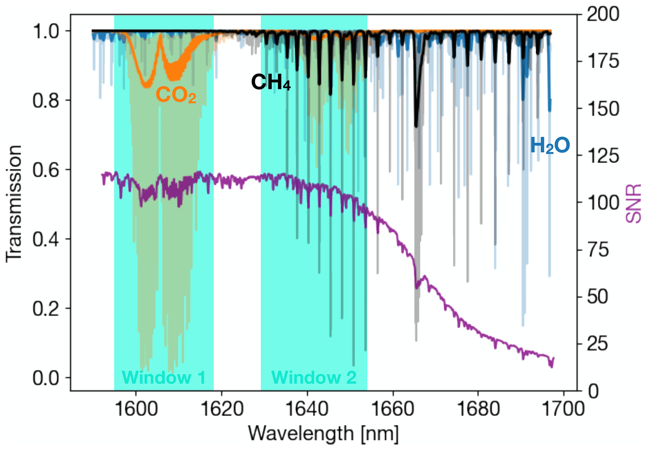
Figure 2Example transmission spectra for a typical MethaneAIR observation (Lambertian albedo: 0.3; solar zenith angle: 30°). Transparent and solid lines represent the spectra before and after convolution with the MethaneAIR instrument line shape, respectively. The signal-to-noise ratio for a typical measurement is also indicated. Windows 1 and 2 indicate the spectral regions used to retrieve CO2 and CH4, respectively.
3.1 Spectroscopy
We model CH4, CO2, and H2O absorption using cross-section lookup tables computed from the GGG2020 spectral database, which is used operationally in TCCON retrievals (Wunch et al., 2011a; Toon, 2022b, a). These tables include speed-dependent Voigt line shapes with line mixing for CO2 (Mendonca et al., 2016) and CH4 (Mendonca et al., 2017). We opt to use GGG2020 to leverage previous validation work evaluating the TCCON retrievals against profiles constructed from in situ aircraft and balloon observations (Wunch et al., 2010; Messerschmidt et al., 2011; Geibel et al., 2012). We scale the retrieved XCH4 using the ratio between the TCCON's GGG2020 air-mass-independent correction factors for CO2 and CH4 (1.0101 / 1.0031). This adjustment is intended to account for the bias induced by the collective effect of GGG2020 line strength errors across the CO2 and CH4 bands. In reality, the factor for MethaneAIR may differ slightly due to vertical-sensitivity differences between it and the TCCON retrievals from which the correction factors are derived. We plan to revisit the question of absolute scaling once we have accumulated more ground-validation overpasses in future campaigns.
3.2 Retrieval configuration
and are derived through the optimization of a state vector (x), which is used to minimize the cost function J(x), expressed as
The above minimizes the balance between the fit residuals of the observations (y) and the forward model (F(x)) and the departure of x from its a priori estimate (xa). The balance of these terms is controlled by the observation covariance matrix (So) and the a priori covariance matrix (Sa). Moreover, γ is an additional regularization parameter that scales the a priori covariance. For retrievals using 5×1 aggregated pixels, we select γ2=10; this selection is guided by an L-curve analysis (Hansen, 2000) and the fact that it produces near-unity sensitivity to CH4 in the boundary layer (see Sect. S1). Based on the same analysis, we found the need to reduce the regularization for retrievals at the native pixel resolution (γ2=50).
Furthermore, y contains radiances from both windows. The initial rationale for their joint optimization is that the weaker CO2 band at 1.645 µm may improve the light path constraint due to its overlap with the target CH4 band. In practice, we have found little difference between this and optimizing the windows independently. Since the proxy method accounts for aerosols via normalization against as the light path constraint, F(x) does not consider scattering and is modeled analytically (Frankenberg et al., 2005). This allows for significantly faster processing compared to the full-physics approach, which explicitly includes aerosols in the state vector. MethaneAIR generates approximately 30 million spectra per flight hour at a native spatial resolution, making speed a significant consideration. The fastest full-physics CH4 retrievals have processing times of ∼ 10 s (Hu et al., 2018), whereas the proxy retrievals are an order of magnitude faster (∼ 1 s per pixel). Thus, the CO2 proxy approach is likely to serve as the backbone for future MethaneSAT operational processing, with a full-physics algorithm applied additionally at an aggregated resolution or in selective cases where a priori CO2 data are expected to be unreliable (e.g., for urban targets).
Table 1MethaneAIR Level-2 algorithm fit settings.
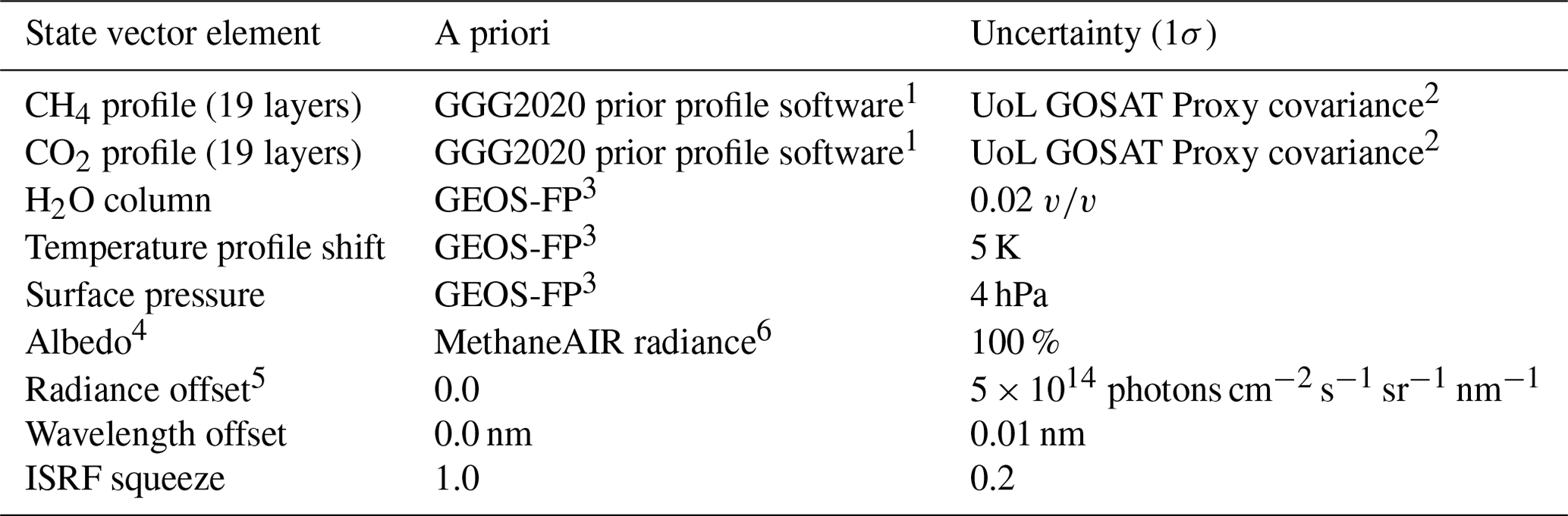
1 Laughner et al. (2022, 2023). 2 Covariance matrix from the University of Leicester GOSAT Proxy retrieval (Parker et al., 2020). 3 Rienecker et al. (2008). 4 A third-order Chebyshev polynomial is used to parameterize the albedo for each window. 5 A first-order Chebyshev polynomial is used to parameterize the radiance offset for each window. 6 Albedo estimated from the average of 5 wavelength pixels centered at 1622.5 nm.
Table 1 summarizes the state vector used in the retrieval. A more detailed description of how the state vector is implemented is provided in the Supplement (Sect. S1). The settings are mostly consistent with those used in similar GHG retrievals (O'Dell et al., 2012; Schepers et al., 2012; Parker et al., 2020). CH4 and CO2 profiles are optimized on a 19-layer vertical grid, consisting of 13 evenly spaced pressure layers from the surface to the tropopause, with a set of fixed pressure levels situated above. We also tested scaling the CH4 and CO2 columns; however, this approach tends to overestimate column XCH4 in cases with large surface enhancements because absorption near the surface is more efficient due to increased pressure broadening, which affects more transparent regions of the spectrum. Scaling the column artificially adds more CH4 to higher altitudes, where CH4 primarily absorbs in the saturated part of the line, requiring the addition of even more CH4 to fit the observed radiance across regions with surface enhancements.
Initial analysis of the first MethaneAIR flight data revealed that the instrument spectral response function (ISRF) was drifting during the course of each flight. The instrument's low F number (3.5) means that small perturbations affecting the instrument, such as changes in the spectrometer's optical-bench temperature or mechanical stresses at the interface between the spectrometer and camera, can lead to significant changes in the way light is focused on the detector. In order to account for this, two additional ISRF squeeze parameters (xsqz) have been included in the state vector to model the ISRF change over both fit windows. The changing width of the ISRF is modeled by squeezing the original wavelength grid from the laboratory-derived tabulated ISRF (ΓTAB(λ)) as follows:
From Eq. (3), xsqz values below (above) unity correspond to stretching (squeezing) the tabulated ISRF. Figure 3 shows the impact of adding the ISRF correction to the spectral fit over a flat background region from the plane's return transit to Colorado from the Midland basin during RF05. When the ISRF squeeze parameter is not included, the fit residuals are significantly larger than what would be expected from the laboratory-derived ISRF (Fig. 3b). Including the ISRF squeeze brings the residuals within the expected noise level, leading to a significant reduction in the XCH4 cross-track bias. In this case, the retrieved scaling factors (xsqz) show changes of up to 30 % in the ISRF width compared to laboratory calibrations. Improvements to the thermal housing of the instrument are planned to improve its stability in upcoming campaigns.
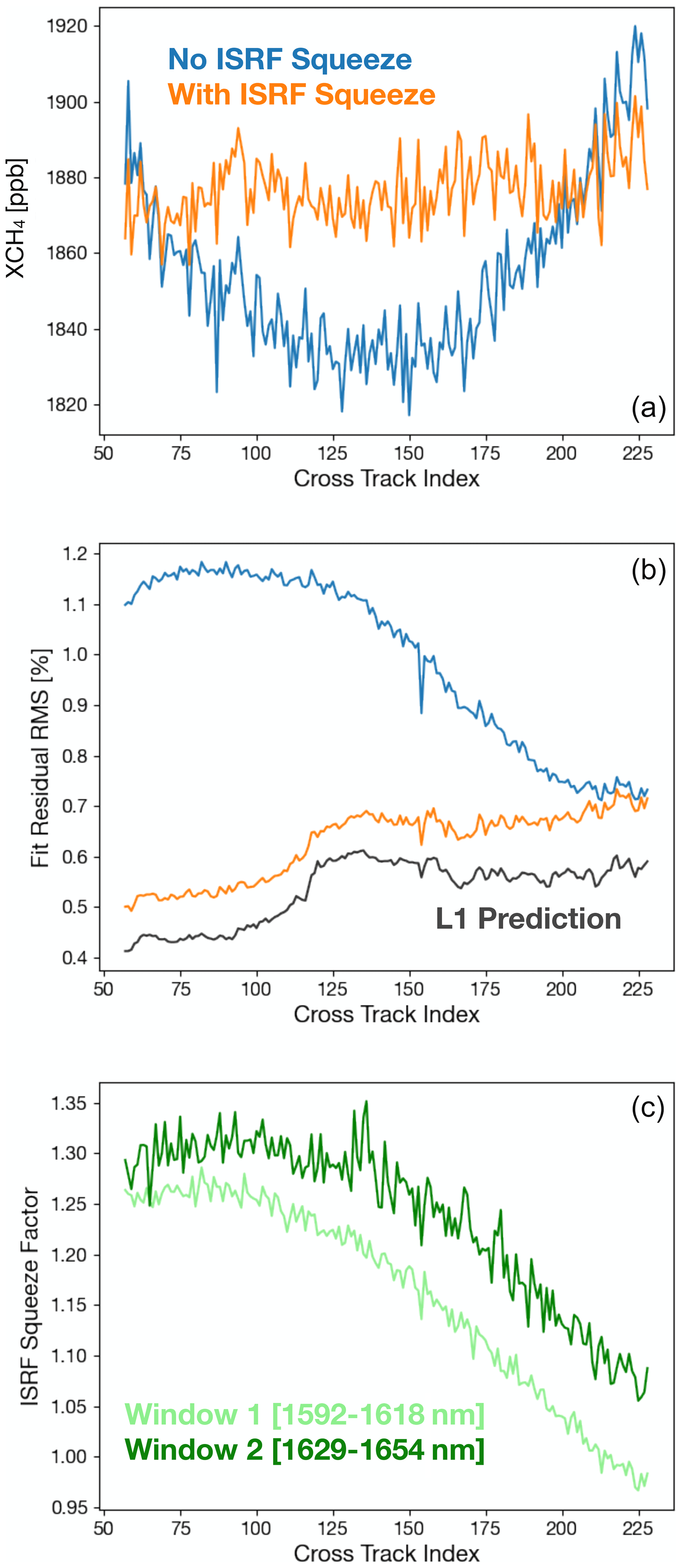
Figure 3Impact of ISRF squeeze on retrieved CH4 derived from observations collected over a clear region during RF05. (a) Cross-track-averaged retrieved XCH4 for retrievals with and without the squeeze factor. (b) Corresponding fit-residual root-mean-square errors (RMSEs). “L1 Prediction” corresponds to the residual RMSE expected from the radiance uncertainty in the Level-1 (L1) product. (c) Retrieved squeeze factors for the CO2 (1595–1618 nm) and CH4 (1629–1654 nm) windows.
3.3 A priori state
The Goddard Earth Observing System – Forward Processing (GEOS-FP) reanalysis (Rienecker et al., 2008) is used as the primary data set for constructing the prior. Profiles of pressure, temperature, and water vapor (H2O) are sampled directly from GEOS-FP. Model observation height differences, computed using digital elevation tiles from Amazon Web Services (Larrick et al., 2020), are used to adjust the GEOS-FP surface pressures to the MethaneAIR ground pixel locations. A priori CO2 and CH4 profiles are calculated using the TCCON's GGG2020 profile construction tool (Laughner et al., 2022), employing GEOS-FP meteorology as input3. The a priori Lambertian surface albedo for each pixel is computed using the transparent region of the observed radiance at 1622 nm, assuming a non-scattering atmosphere. The a priori uncertainties for most state vector elements are based on an Orbiting Carbon Observatory-2 (OCO-2) Atmospheric CO2 Observations from Space (ACOS) algorithm (O'Dell et al., 2012). The profiles for the CH4 and CO2 covariance matrices are from the University of Leicester (UoL) GOSAT Proxy retrieval (Parker et al., 2020).
3.4 Cloud screening
Cloud-impacted observations are rejected using a cloud screening algorithm modeled on the OCO-2 A-band Preprocessor (Taylor et al., 2016). Here, surface pressure is retrieved from the instrument's O2 band, assuming a cloud-free atmosphere. In this case, large deviations from the a priori pressure can be interpreted as being due to clouds. The algorithm similarly uses retrieved vertical column densities of CO2 and CH4 to screen out clouds with high optical depths, which cause distinct decreases relative to their priors (Fig. 4). The screening flags are combined with the oxygen-band retrieval using a naive Bayes classifier (Heidinger et al., 2012), allowing the screening algorithm to function even when there are no overlapping oxygen-band data. More details will be provided in a paper currently in preparation.
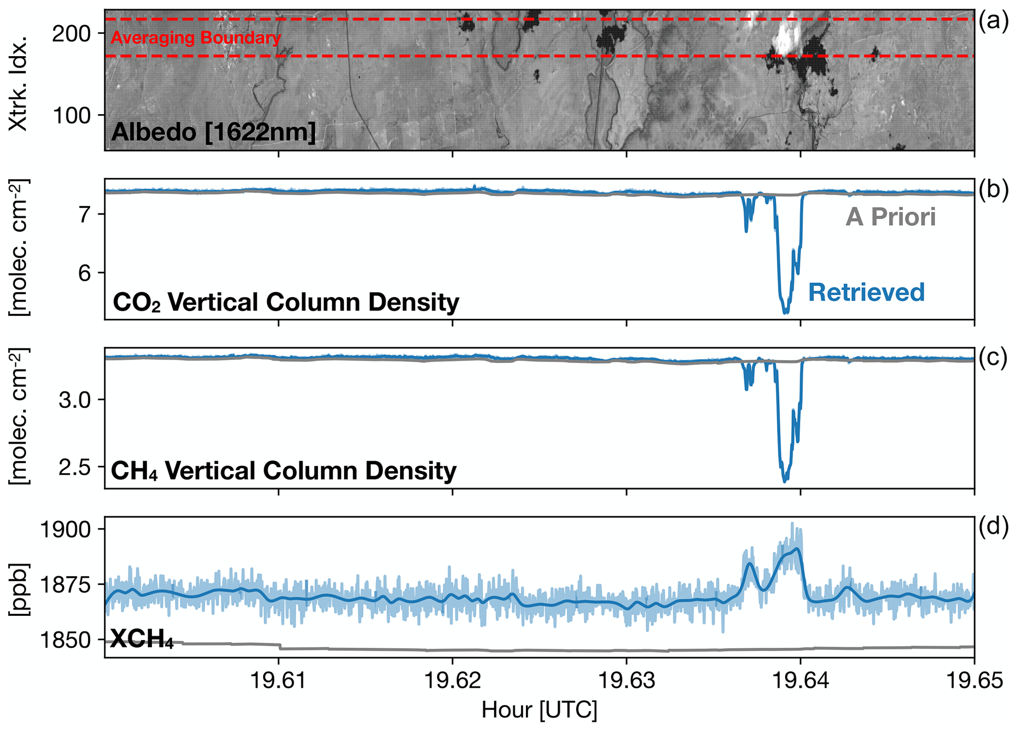
Figure 4XCH4 retrieved in the presence of a low-altitude cloud during RF06. Panel (a) shows a grayscale albedo image estimated from the MethaneAIR radiance. Panels (b)–(d) show the cross-track median values of the CO2 vertical column density, the CH4 vertical column density, and XCH4 from the MethaneAIR retrieval, respectively. The solid blue lines represent the 5-fold cross-validated smoothed spline values. The a priori values are shown in gray. “Xtrk. Idx.”: cross-track index.
4.1 Evidence of time-dependent cross-track bias
In the previous section, it was shown that the in-flight ISRF can differ significantly from the table derived from on-ground laser calibration measurements, with changes of up to 30 % in the FWHM (Fig. 3). This change slowly evolves over the course of a flight. Figure 5c1 shows the time evolution of the ISRF squeeze factors for each spectral fit window retrieved from RF05. Early on in the flight, each ISRF squeeze factor (xsqz) is close to 1, indicating that the ISRF is close to the nominal calibration. As the flight continues, the ISRF width gradually narrows (xsqz>1), with the effect becoming more pronounced at the side of the detector corresponding to the lower cross-track indices. Similar ISRF squeeze changes were observed during the other flights.
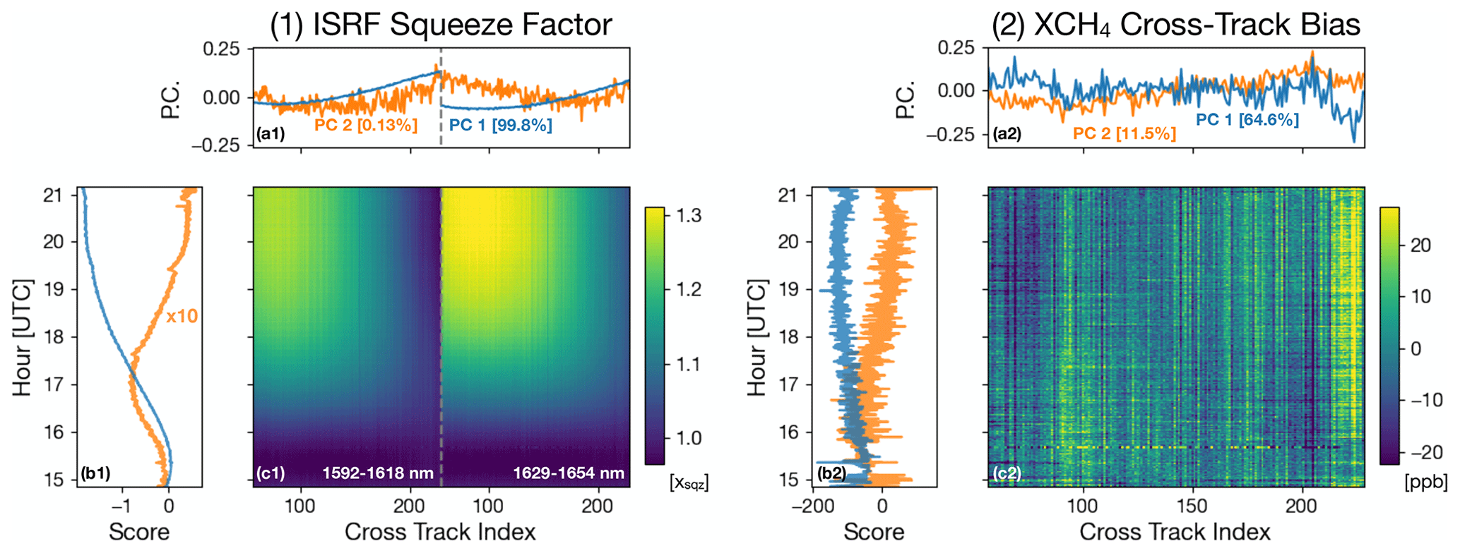
Figure 5Relationship between retrieved ISRF squeeze factors and XCH4 cross-track bias during RF05 (3 August 2021). The contour plots illustrate the time evolution of the ISRF squeeze factors for each retrieval window (c1) and the XCH4 cross-track bias derived from the small-area approximation (c2). Panels (a1) and (a2) show the first two principal components for the combined ISRF squeeze parameters and XCH4 bias, respectively. The corresponding component scores are shown in panels (b1) and (b2).
In order to better understand the temporal evolution of the ISRF, we applied principal component analysis (PCA) to the ISRF squeeze factors from both the CO2 and CH4 fit windows simultaneously. PCA is a common dimensionality reduction technique that reconstructs a multidimensional data set from a smaller number of principal components. Let s(ti)∈ℝ2n represent the vector containing the ISRF squeeze factors from both windows, each housing n cross-track pixels, at the tith time. Moreover, s(ti) is reconstructed using the npc principal components (pj∈ℝ2n), scaled by the scores cj(ti):
where is the mean ISRF squeeze at each cross-track pixel. The first principle component (p1) is chosen to account for the largest possible variance in the data set, and each successive component accounts for the highest possible variance under the constraint that it is orthogonal to the previous ones.
Figure 5a1 and b1 shows the first two principal components and their scores, respectively, for the ISRF squeeze factors. The first principal component explains almost all the variance in the ISRF squeeze factors (99.8 %). It is also highly correlated with the temperature of the environment surrounding the instrument (Fig. 6). This strong relationship suggests that the ISRF changes are caused by the cooling of critical optical components of the spectrometer, such as the foreoptic lens adjacent to the cold viewport window glass. These temperature changes can defocus light at the FPA, leading to observable changes in ISRF width. The fact that the ISRF changes cause the temperature to lag by ∼ 0.75 h also supports this hypothesis (inset in Fig. 6) as this is expected due to the thermal inertia of the optical components.
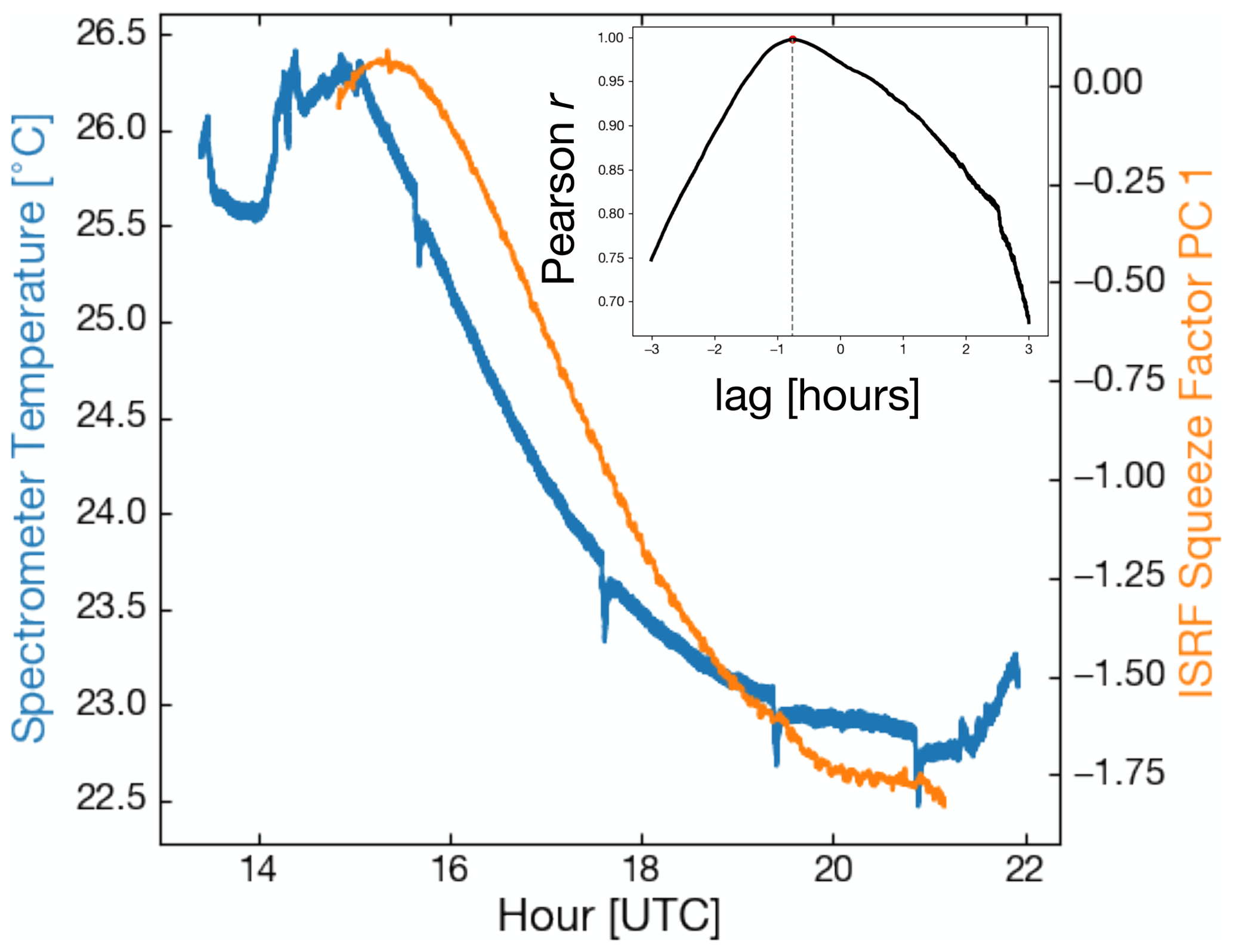
Figure 6Comparison of the time series for the first principal component of the ISRF squeeze factor (see text) and the spectrometer temperature from RF05. Here, spectrometer temperature refers to the temperature recorded by a probe outside the instrument but within the thermal housing that isolates the spectrometer from the plane cabin. The lag correlation between the two variables is shown in the inset and is defined as the value of Pearson's r computed between the spectrometer temperature (Tspec(t)) and the ISRF principal component shifted by the lag value (c1(t+tlag)).
It is unlikely that squeezing the laboratory-derived tabulated ISRF fully accounts for the change in ISRF shape induced by defocusing. The gradual drift in instrument focus may lead to a time-dependent XCH4 cross-track bias, which we attempt to derive using a small-area approximation (O'Dell et al., 2018). This assumes that XCH4 over a small area is constant. In this case, we derive the background XCH4 for every cross-track index by computing its median value over consecutive 10 s (∼ 2 km) intervals. The segment interval is chosen to be short enough for the sequence of retrieved squeeze values to capture temporal changes in the cross-track-bias pattern but long enough to reduce the impact of plumes; however, it should not be so long that it entrains topographic gradients. Let XCH be the retrieved XCH4 for a 10 s segment g at the cross-track index ix and the along-track index it. The cross-track bias at the cross-track index ix for the granule (Bg(ix)) is estimated as follows:
where “med” and “mean” denote the median and mean, respectively, and “:” denotes the array axis along which the operation is performed. The XCH4 cross-track bias for RF05 is shown in Fig. 5c2, along with its PCA decomposition (Fig. 5a2 and b2). The derived bias pattern shows a temporally constant set of index-to-index cross-track stripes over the course of the flight, with an additional slowly evolving bias pattern smoothed over the entire detector array. The relatively constant pattern is likely due to instrument slit inhomogeneities and is a common feature of other 2D grating spectrometers, e.g., MODIS (Rakwatin et al., 2007), the Ozone Monitoring Instrument (OMI; Boersma et al., 2011), and TROPOMI (Borsdorff et al., 2019).
The temporal evolution of the broader bias pattern strongly correlates with changes in ISRF width. This correlation can be seen more clearly in the ISRF squeeze and PCA scores for the XCH4 cross-track-bias patterns (Fig. 5b1 and b2). The scores of the leading ISRF and XCH4 bias principal components (PCs) are highly correlated in terms of time (Pearson's r value of 0.76). Although the second ISRF PC explains only a small portion of the total ISRF variability (0.13 %), its scores are highly correlated with the first two XCH4 bias PCs (Pearson's r values of 0.77 and 0.69, respectively). This suggests that subtle ISRF changes captured by the less-dominant PCs could contain valuable information for modeling the XCH4 bias.
4.2 MethaneAIR cross-track-bias correction algorithm
Since there is an underlying physical connection between the XCH4 cross-track bias and ISRF squeeze parameters, errors associated with the small-area approximation can be further reduced by constructing a regression model that relates these two retrieved quantities. As the noise in retrieved ISRF squeeze parameters is lower than that in the retrieved XCH4, this approach will also improve the precision of cross-track-bias prediction compared to directly applying the values shown in Fig. 5c2. Here, we create a linear model of the cross-track bias (n pixels) from a total of t segments, each containing 10 s of observations. We predict the XCH4 biases (the “response” variables) derived from the small-area approximation () against the retrieved ISRF squeeze factors (the “predictor” variables) combined from both windows ().
where β represents the transformation between S and B and is determined using partial least-squares (PLS) regression (Wold et al., 2001). In this case, ordinary multiple least-squares regression is not appropriate as it assumes that there is no correlation between the squeeze factors at different cross-track positions. One possible way around this involves creating a multiple-regression model using a truncated set of principal components (e.g., those shown in Fig. 5). However, the principal components that are omitted from the regression could still contain valuable information explaining the variation between the response and predictor variables. Indeed, the strong correlation between the scores of the second ISRF PC and those from the XCH4 bias data set, as previously discussed, suggests that this may not be the most appropriate method.
PLS regression overcomes this PCA truncation issue by finding component pairs between the predictor and target data sets that maximize the covariance between them. This contrasts with PCA regression, where components are independently chosen to maximize their own explained variance. The algorithm works iteratively by first identifying the covariance-maximizing predictor–response component pair, subtracting the variation captured by these from the data sets, and then repeating the process. The process is ideally terminated after a sufficient number of components are included to explain the true variation in the response data set. Here, we determine this component number using k-fold cross-validation.
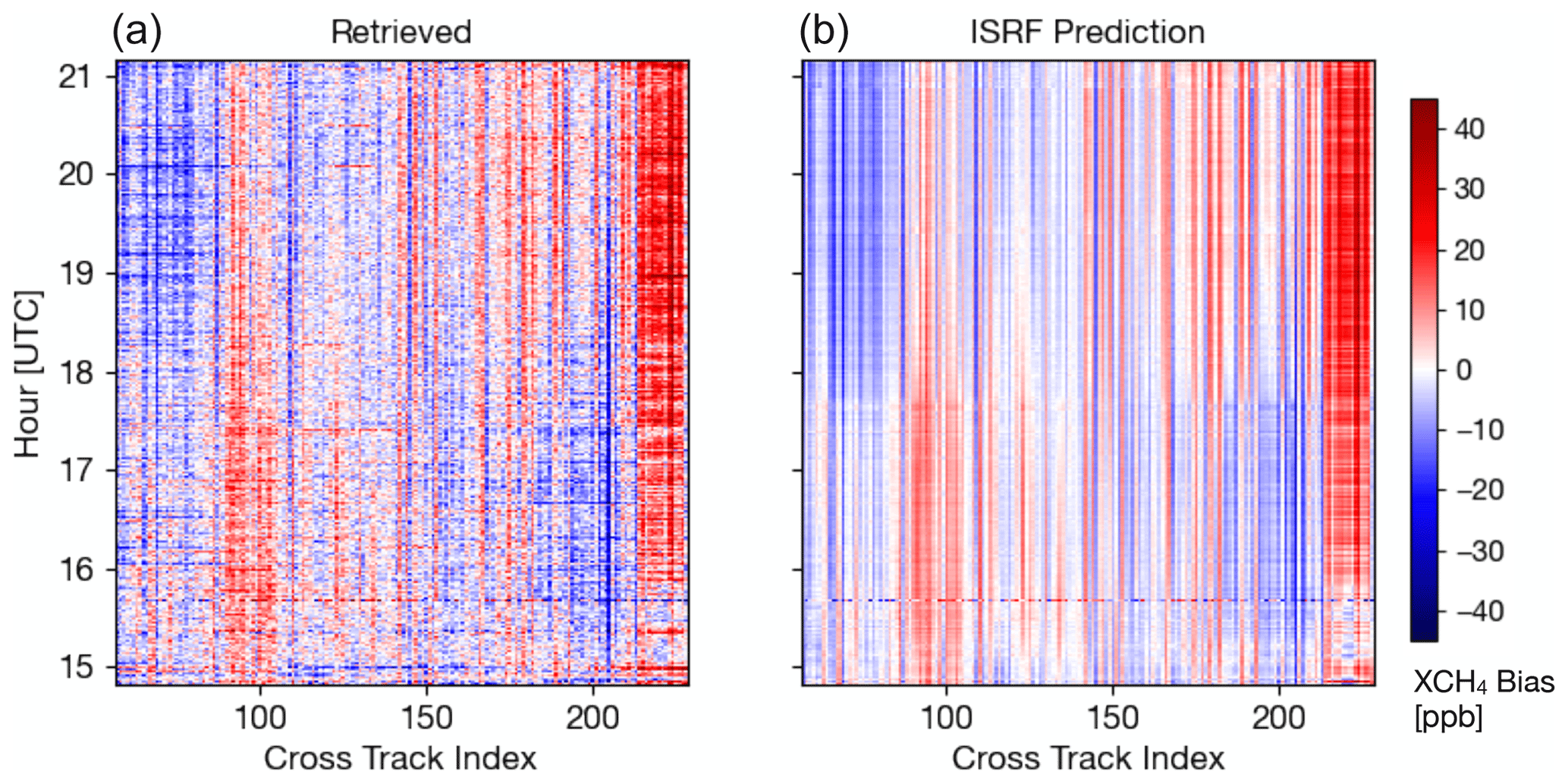
Figure 7XCH4 cross-track-bias estimate using the small-area approximation (a), which is subsequently refined using the PLS regression model (b). The PLS regression model (Eq. 7) uses the retrieved ISRF squeeze factors to predict the data used in panel (a), preserving only the sources of variability related to temperature-induced defocusing effects.
Figure 7 compares the cross-track bias derived from the small-area approximation with that predicted by the regression model. It can be seen that the regression model reduces the noise in the original data set and removes some spurious features that extend over multiple cross-track positions, which are likely due to real XCH4 enhancements. The updated bias estimate is also less noisy due to the higher precision of the retrieved ISRF squeeze factors relative to the XCH4 values used in the small-area approximation.
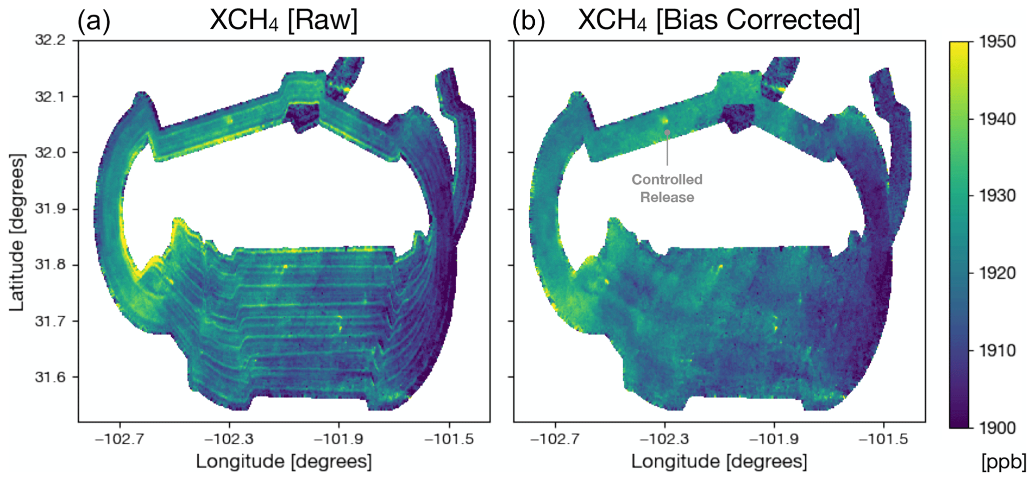
Figure 8XCH4 retrieved during RF05 (3 August 2021) and gridded at a 20×20 m2 resolution (a) prior to destriping correction and (b) after destriping correction. Here, the aircraft is traveling in a clockwise loop, with the northern segments overlapping to target a controlled release.
Figure 8 compares the MethaneAIR XCH4 retrievals over the Midland basin from RF05, highlighting the results obtained before and after the stripe correction was applied. We applied the bias correction to a given observation by temporally interpolating the PLS-regression-derived bias (Fig. 7b) to align with the time of observation. In principle, the retrieved ISRF at the observation time could also be directly inputted into the regression model (Eq. 7). In practice, we found that the former method performed better because (1) the ISRF varied smoothly over time and (2) the latter method induced additional noise due to the 10-fold lower precision of the single-pixel ISRF values compared to the 10 s averages used in the PLS regression model. Figure 8 shows that the bias correction is able to remove the cross-track striping apparent in the uncorrected data while preserving observations of plumes from O&G infrastructure within the basin and at the controlled-release site.
5.1 EM27/SUN ground validation
Surveying CH4 across an O&G basin requires 2–3 h of MethaneAIR observations at a nominal above-ground observation altitude of 12 km. It is critical that the retrieved XCH4 is free of significant systematic drifts as such drifts could yield artificial gradients within the mapped areas and ultimately reduce the accuracy of emission inversion. Given the changes in the ISRF described in the previous section, such drifts are certainly possible and can be quantified using the aircraft overpasses of the EM27/SUN spectrometer sites conducted over the course of the campaign. Figure 9 shows the comparison between the MethaneAIR and EM27/SUN retrievals for the five flights that intersected the ground sites. For each EM27/SUN overpass, we colocate MethaneAIR retrievals within a 0.05° latitude–longitude box around the site location. To remove the influence of the GGG2020 CO2 prior from the comparison, we use XCO2 observed by the EM27/SUN instead of a priori GGG2020 XCO2 when calculating MethaneAIR XCH4 from the retrieved vertical column densities (XCO2,0; Eq. 1). To reduce differences between MethaneAIR and EM27/SUN retrievals caused by differences in their respective a priori CH4 profiles and averaging kernels, we adjust MethaneAIR to the EM27/SUN prior and smooth the EM27/SUN observation by the MethaneAIR averaging kernel, following Wunch et al. (2011b) (Appendix A). Furthermore, we restrict the comparison to retrievals in which the a priori surface pressure falls within 10 hPa of the pressure measured at the EM27/SUN location. This is particularly important for the NCAR Boulder site used for the summer campaign, where there is significant topographic variation associated with the Rocky Mountains immediately to the west. MethaneAIR retrievals are also screened for poor spectral fits4 and low signal by rejecting pixels in which the degrees of freedom for signal (DOFS) for CO2 and CH4 retrieval drop below 1, indicating a poor column constraint. Cloud-contaminated pixels are filtered using the algorithm in Sect. 3.4.
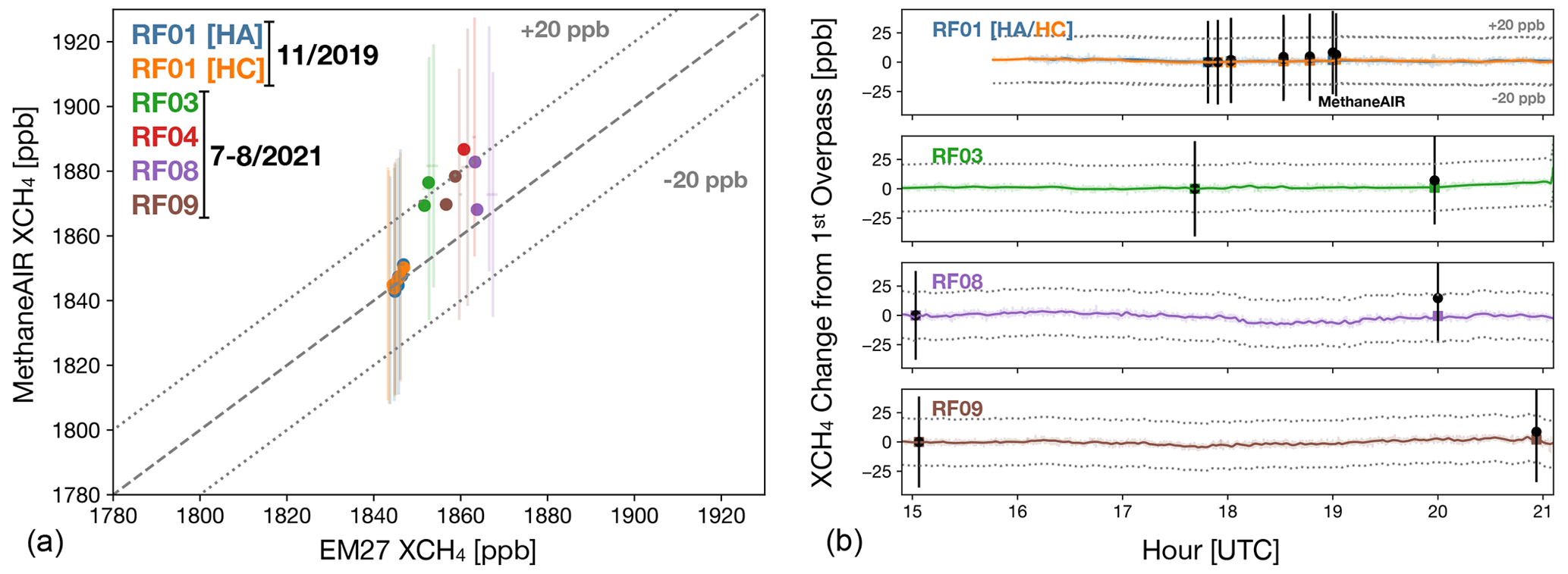
Figure 9(a) Comparison of colocated MethaneAIR and EM27/SUN retrievals of XCH4 (see text for the colocation criteria). Error bars represent the 1σ XCH4 cross-track variability within the 0.05° colocation region (since there are >3000 pixels for each MethaneAIR average, the XCH4 random error is negligible). HA and HC refer to the two EM27/SUN spectrometers used in the first flight campaign. The dashed lines corresponding to ±20 ppb indicate a ∼1 % accuracy level. The MethaneAIR XCH4 values were adjusted to align with the EM27/SUN CH4 profile, and the EM27/SUN retrievals were smoothed with the MethaneAIR CH4 averaging kernels, following Wunch et al. (2011b). (b) Time series illustrating the relative XCH4 drift between MethaneAIR retrievals (black dots) and EM27/SUN retrievals (colored lines) following the first overpass for flights with multiple overpasses. The colored squares indicate the EM27/SUN retrievals smoothed with the MethaneAIR CH4 averaging kernels. The XCH4 value at the time of the first overpass is subtracted from each data set to visualize the relative drift.
In general, there is good absolute agreement between the MethaneAIR and EM27/SUN retrievals. The mean bias from the winter flights was 2 ppb, with minimal drift in MethaneAIR XCH4 for the five overpasses over a 70 min interval (Fig. 9b). The mean bias for the summer campaign increased to 13 ppb. This could be partially due to the different EM27/SUN spectrometers used for the summer and winter campaigns, although instrument-to-instrument variations have been shown to be within 0.3 % (∼ 6 ppb) (Alberti et al., 2022). The summer observations were also influenced by visible haze from intense fires in the western US. However, this haze was not visible in the grayscale imagery generated from MethaneAIR data, and there is no evidence of strong correlations between retrieved XCH4 and surface albedo, which is a typical indicator of aerosol presence (Butz et al., 2010). Thus, the size distribution of the smoke aerosols present was likely small enough to avoid causing strong scattering in the shortwave-infrared region.
Differences in the vertical sensitivity of the MethaneAIR and EM27/SUN retrievals could explain the flight-to-flight differences in the summer campaign. Figure 10 shows the column averaging kernels for the two sensors from the RF08 overpasses, which represent observations made at high (57°) and low (28°) solar zenith angles. The MethaneAIR retrieval is less sensitive to the air mass above the aircraft as the solar light that returns to the sensor traverses the layer above only once. In contrast, the EM27/SUN retrieval exhibits greater sensitivity to stratospheric differences. The uncertainties in the GGG2020 profiles of background CH4 are largest in the stratosphere, as demonstrated by comparisons with in situ, balloon-borne AirCore profiles (Karion et al., 2010), which produce RMSE errors of ∼ 30 ppb at the tropopause, peaking at ∼ 80 ppb at ∼ 100 hPa (Laughner et al., 2023). This translates to a 1σ variability of at least ∼ 5 ppb, induced by the different stratospheric instrument sensitivities shown in Fig. 105.
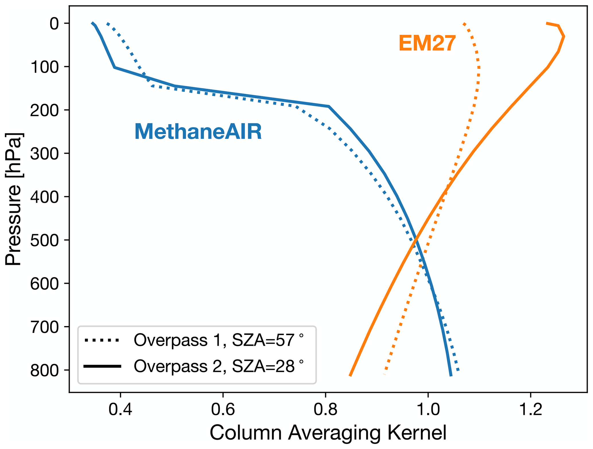
Figure 10MethaneAIR and EM27/SUN column averaging kernels for the two MethaneAIR overpasses from RF08. The MethaneAIR kernels are computed from the average of the retrievals colocated with the EM27/SUN site. SZA: solar zenith angle.
The summer flights showed a consistent positive XCH4 drift relative to the EM27/SUN retrievals, ranging from 1.0 ppb h−1 for RF09 to 3.2 ppb h−1 for RF08 (Fig. 9b). This drift correlates with the temperature-induced changes in the ISRF described in the previous section (Fig. 5). The drift is likely due to the ISRF not being perfectly modeled by the ISRF squeeze factor. Since the time evolution of the ISRF squeeze factors showed a similar pattern for each flight, this could also explain why the sign of the drift was always positive. Efforts are currently being made to improve the temperature stability of the instrument in flight for future campaigns. For now, we note that drifts at these levels should still allow for the inference of emissions from diffuse CH4 sources since the total drift over the time it takes to map a target area (1–2 h) is approximately 1 order of magnitude lower than the XCH4 gradients typically observed (see Sect. 7).
5.2 Intercomparison with TROPOMI
To evaluate a wider subset of MethaneAIR retrievals, we also took advantage of the greater coverage provided by the TROPOMI satellite instrument (Hu et al., 2018). Figure 11 compares TROPOMI XCH4 retrievals from the standard V1 product (Hu et al., 2018) to XCH4 retrievals from MethaneAIR obtained during RF06, averaged across overlapping TROPOMI pixels within a ±1 h time interval. The TROPOMI data were destriped using the median filter method described by Liu et al. (2021). The overlapping retrievals extend from the Permian Basin and continue along the transit back to the base airfield in Broomfield, Colorado. MethaneAIR captures the Permian hotspot and the large-scale latitudinal gradient observed by TROPOMI.
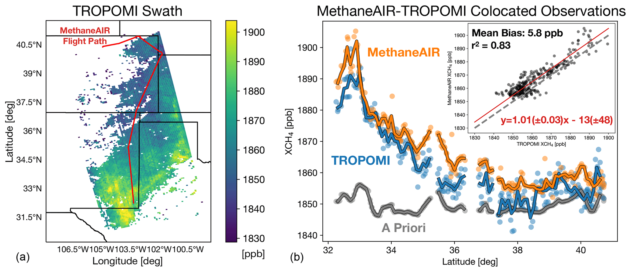
Figure 11Comparison of colocated MethaneAIR and TROPOMI XCH4 retrievals collected during RF06. (a) TROPOMI XCH4 retrievals (orbit no. 19769), filtered using quality assurance values >0.5 and destriped using the algorithm described in Liu et al. (2021). The overlapping MethaneAIR flight path situated within 1 h of the TROPOMI overpass is shown in red. (b) Comparison with MethaneAIR retrievals averaged across the overlapping TROPOMI pixels. The inset shows a scatterplot of the matched retrievals along with the RMA regression fit (red).
The correlation between retrievals is high (reduced-major-axis (RMA) regression r2=0.83), and the absolute mean bias is small (5.8 ppb). The offset between retrievals can be attributed to the MethaneAIR XCH4 bias induced by the CO2 prior used in the proxy normalization, with uncertainties of ∼ 1 % in the troposphere, translating to an XCH4 retrieval uncertainty of ∼ 14 ppb. The slope of the regression from the colocated retrievals is 1.01, which is within the uncertainty of the linear regression. Since the enhancement over the Permian Basin drives the regression slope, the near-unity slope indicates that both would yield similar total basin emission estimates.
5.3 Evaluation against surface albedo
GHG retrievals are typically correlated with other geophysical parameters, with surface reflectance usually having the strongest correlation (O'Dell et al., 2018; Lorente et al., 2021). This correlation arises due to biases induced by light path modifications from aerosol scattering, which strongly depend on the underlying surface (Butz et al., 2010). For instance, aerosol layers over dark surfaces tend to shield radiation, preventing it from penetrating below them, while a layer over a bright surface may enhance the mean photon path below the layer due to multiple scattering between the surface and aerosol layer. Following Lorente et al. (2021), we investigate the correlation between XCH4 and albedo by analyzing the retrievals over small background regions. We divide the return leg of RF06 between 34.8 and 40° latitude into 3 min (∼ 30–40 km) segments, which are small enough to assume XCH4 is constant across the segment (see Fig. 11). For the albedo, we use the a priori reflectance estimate obtained from the observed radiance at 1622 nm. In each segment, the XCH4 bias due to surface reflectance is derived by subtracting the average XCH4 computed from a bin with a width of 0.02, centered at an albedo of 0.2. This value was chosen as it typically corresponds to where aerosol-induced biases are at a minimum (Aben et al., 2007; Guerlet et al., 2013).
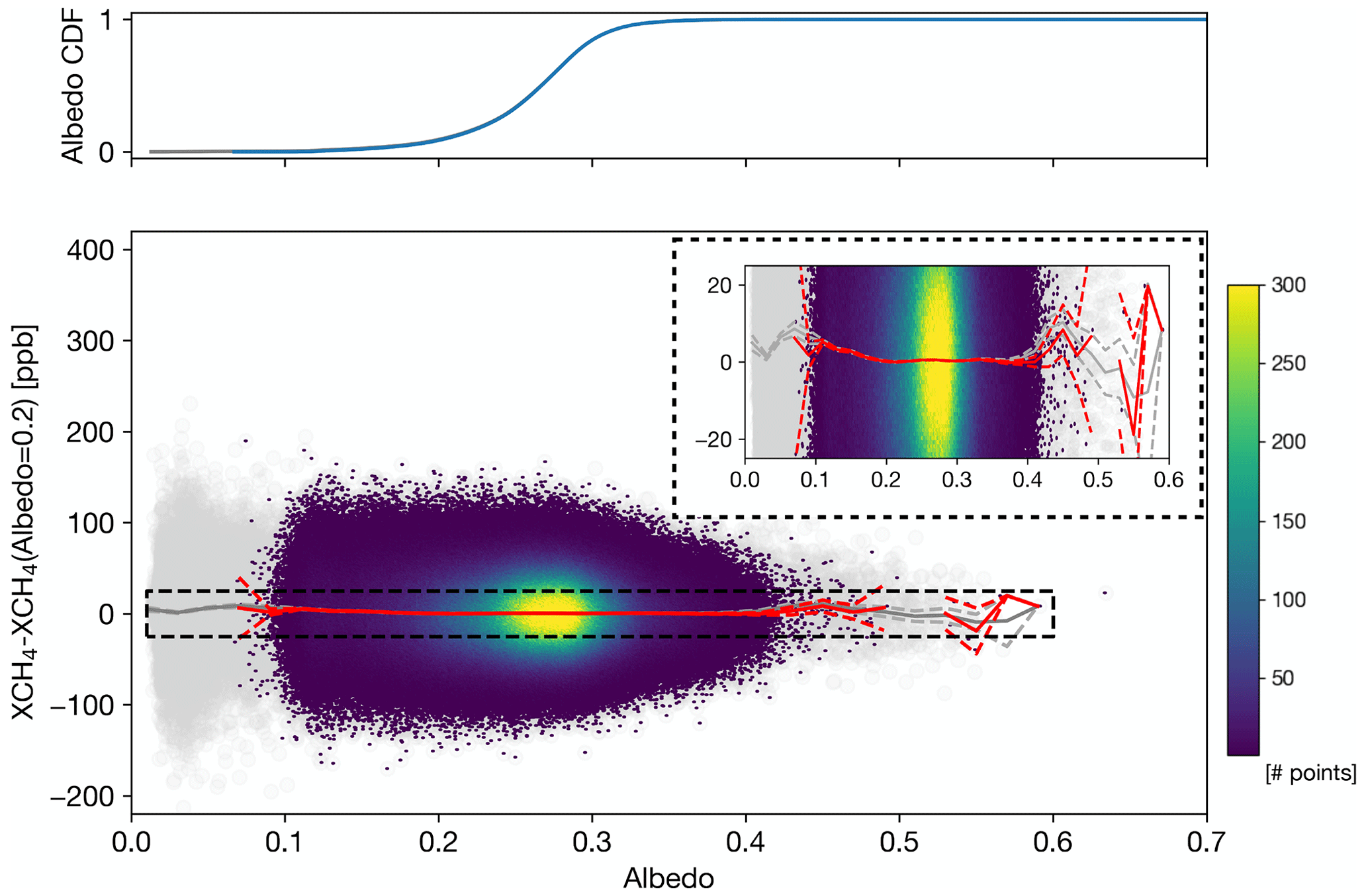
Figure 12The dependence of XCH4 on surface albedo. The relationship between the XCH4 bias and albedo, derived using small-area approximation (see text), is shown for the return leg of RF06 between 34.8–40° N. Albedo is computed from the radiance at 1622 nm under clear-sky conditions. The XCH4 bias (y axis) is derived by subtracting the mean XCH4 for albedos between 0.19–0.21. The gray points represent data excluded from the cloud screening algorithm and retrieval quality flags. The gray and red lines show the binned averages computed in albedo increments of 0.02 before and after cloud screening, respectively, with dashed lines indicating the 2σ bin sample mean uncertainty. The cumulative distribution function (CDF) of albedo is shown above the main panel, with gray and blue lines representing all data and cloud-screened data, respectively).
Figure 12 shows the albedo-induced XCH4 biases derived from the return leg. Here, the data were screened using the cloud algorithm described in Sect. 5.1. For the screened data, there is almost no albedo dependence over the albedo range of 0.2–0.4, which corresponds to 90 % of the total observations. The bias then slowly increases to 5 ppb as albedo decreases from 0.2 to 0.1, possibly due to residual cloud contamination. This contrasts with the TROPOMI full-physics retrievals, which show a bias increase of 1.5 % (∼ 28 ppb) over this range (Lorente et al., 2021, 2023). The stronger dependence in TROPOMI may be due to the spectral separation between the oxygen A-band (757–774 nm), used as the light path constraint, and the target CH4 band (2305–2385 nm), which increases susceptibility to errors induced by retrieval assumptions regarding aerosol optical properties. Nevertheless, the albedo dependence for MethaneAIR is lower than anticipated, given that observations collected during the campaign were often obtained over regions blanketed by haze from the long-range transport of smoke from fires in the western United States and Canada. Since a large fraction of this may have been in drier air in the free troposphere, the size distribution may have been small enough for the aerosol optical depth to be insignificant at 1600 nm.
Figure 12 also demonstrates the importance of cloud screening. Below an albedo of 0.02, the XCH4 bias increases, peaking at 9 ppb at an albedo of 0.05. This bias is due to cloud shadows and other low-signal scenes, such as those over water, where the retrieved XCH4 is heavily influenced by the a priori information. The peak occurs due to the fact there is less spectral information for constraining CO2, and, as a result, it tends toward its prior value at a higher albedo than that observed for CH4. This can be clearly seen in the profile DOFS for both species (Fig. S3), which drop below 1 at albedos of 0.18 and 0.06 for CO2 and CH4, respectively. In general, the sign and magnitude of this bias will be scene dependent and determined by the a priori profile bias along with additional light-path modifications induced by aerosol scattering. In practice, since the degree of regularization is dependent on the radiance, the albedo threshold will also depend on the location and time of the measurement. At first order, this will largely be a function of the solar zenith angle (SZA), assuming most surfaces are approximately Lambertian. For the scene shown here, the SZAs ranged from 22–24°, with 90 % of the radiance expected for a SZA of 0°, and the cloud screening and quality filtering remove points below an albedo of approximately 0.1. Thus, we expect the regularization threshold to roughly follow (SZA), corresponding to albedo thresholds of 0.13 and 0.18 at 45 and 60°, respectively. In practice, if these thresholds are too high, the regularization parameter (γ; Eq. 2) can be retuned at the cost of worsening the measurement precision. The choice here has been optimized to avoid regularization biases over the primary observation targets for this campaign (see Sect. S1).
6.1 Plume mask algorithm description
The previous section showed that the main error in the flight retrievals is due to random noise. We estimate the precision of the retrievals using 5×1 aggregated pixels to be 35 ppb by calculating the standard deviation of the XCH4 retrieved over background locations, as shown in Fig. 12. This value is consistent with our estimate for the native resolution of MethaneSAT (Sect. S2.1), which has a similar signal-to-noise ratio (SNR) as the MethaneAIR retrieval using 5×1 aggregated pixels. These noise levels reduce MethaneAIR's ability to detect small-scale XCH4 gradients. To reduce random noise, we apply the Chambolle total variance (TV) denoising filter (Chambolle, 2004) to the retrieved XCH4 images. The TV filter works by minimizing the following cost function between the original (f) and smoothed (g) images:
The cost function penalizes departures from the original image, measured by the least-squares difference (E(f,g)). Smoothing is controlled by V(g), which measures adjacent pixel differences in the image. The degree of smoothing is controlled by the smoothing parameter λ. The filter was chosen for its favorable properties, ensuring that the resulting smoothed XCH4 fields can be used to estimate CH4 point-source emissions (Q) without inducing additional bias. Here, and for MethaneSAT, the integrated-mass-enhancement (IME) method (Frankenberg et al., 2016; Varon et al., 2018) is the primary method used to estimate Q:
Here, the IME is the integrated CH4 mass of the plume. The effective wind speed (ueff) and plume length scale (L) are parameters that account for the impacts of turbulent diffusion on the observed plume extent. L is estimated by taking the square root of the plume area. In practice, ueff is determined from an ensemble of large-eddy simulations as a function of the 10 m horizontal wind speed (u10). For MethaneAIR, u10 is determined by a large-eddy simulation of the target scene at the time of observation (Chulakadaba et al., 2023). The TV filter has some important properties for the unbiased estimation of Q. First, it is conservative, meaning that the smoothing does not bias the IME estimate. Second, it has an edge-preserving functionality, which means that it does not bias the estimate of L.
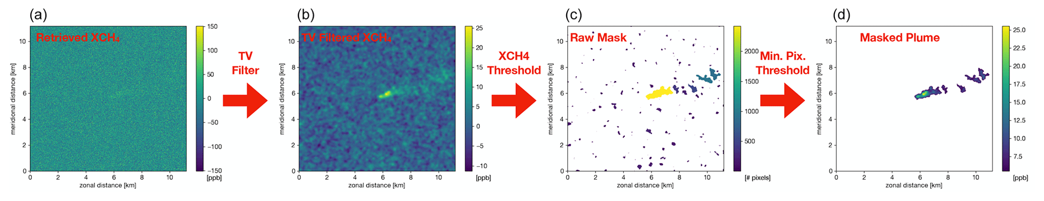
Figure 13Schematic of the plume-masking procedure. Panel (a) shows a synthetic 20×20 m2 retrieval using MethaneAIR precision for a plume from a 200 kg h−1 point source, simulated using a Weather Research and Forecasting large-eddy simulation (WRF-LES). (b) A Chambolle TV image filter is then applied to the retrieved XCH4 map. (c) Next, a threshold XCH4 is determined using the trimmed mean and standard deviation of the TV-filtered image to generate a raw plume mask. The threshold here is set at 2 standard deviations above the mean. (d) Finally, small clusters of pixels (artifacts of the random error in the image) are removed to yield the final masked plume.
The IME method also requires an algorithm for plume masking. Figure 13 shows the approach adopted here. First, the TV filter is applied to the noisy image. The background XCH4 is then estimated by taking the 3σ iteratively clipped mean of the denoised image. An initial mask is computed by flagging mole fractions that are 2 standard deviations above this background. The final plume mask is computed by discarding flagged pixel clusters that contain fewer than a threshold number of pixels (nmin). This threshold depends on the degree of smoothing applied by the TV filter.
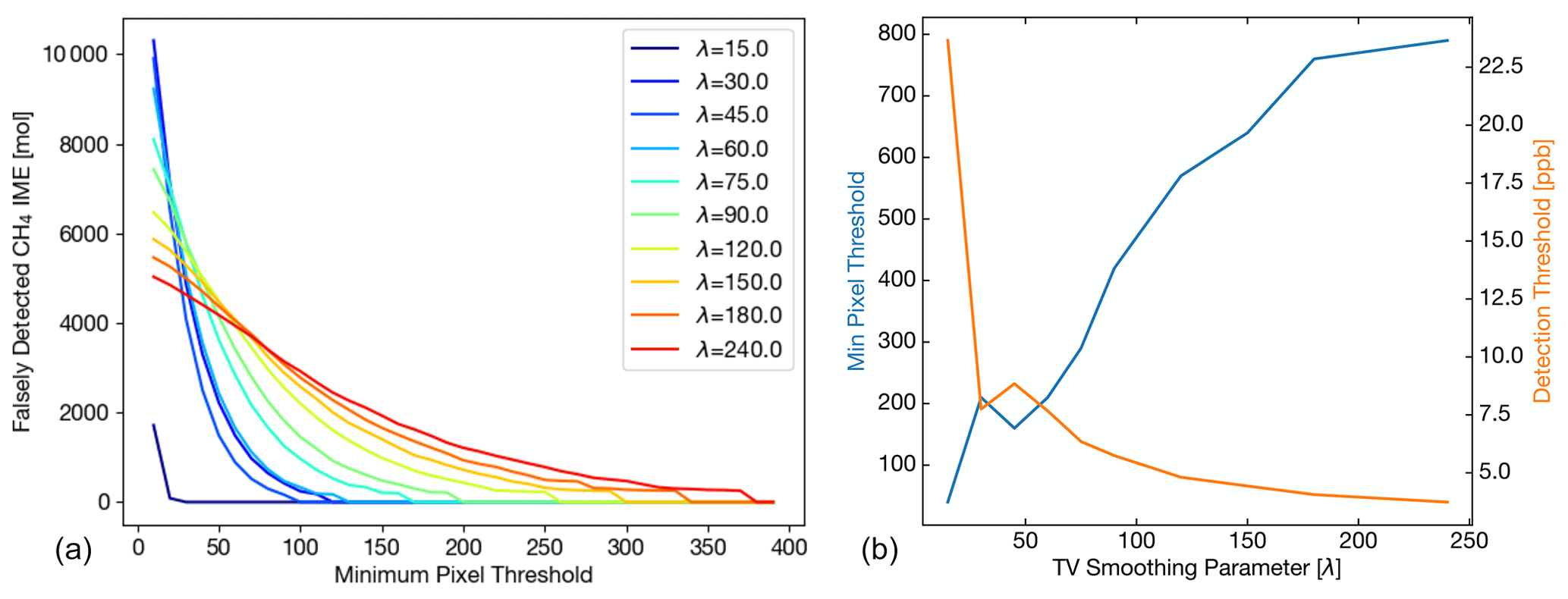
Figure 14Determination of plume mask parameters from plume-free synthetic MethaneAIR retrievals. Panel (a) shows the falsely detected plume mass for different levels of TV smoothing as a function of the minimum pixel cluster threshold. Panel (b) shows the minimum pixel threshold required to exclude falsely detected plume mass as a function of smoothing weight (blue line). The XCH4 plume threshold versus smoothing weight is also shown (orange line).
To optimize the choice of λ and the pixel threshold, we applied the TV filter to a set of 300 plume-free synthetic noisy retrievals, generated from Gaussian random noise at the MethaneAIR precision of 35 ppb, corresponding to the resolution of 5×1 aggregated pixels. Figure 14a shows the falsely detected plume mass as a function of the pixel cluster threshold for various levels of smoothing. As smoothing increases, the random artifacts in the image spread in terms of area and decrease in terms of XCH4, lowering the XCH4 detection threshold. As a result, lower levels of smoothing require a higher nmin in order to filter out the falsely identified mass. The smallest threshold needed to fully eliminate the falsely identified plume mass is shown in Fig. 14b, along with the XCH4 detection threshold determined from the variance of the filtered image. At low smoothing levels (λ<45), the XCH4 detection threshold decreases sharply, exhibiting only small increases in nmin. Beyond this point, the pixel threshold limit continues to increase, showing little improvement in the XCH4 threshold. We thus set the plume detection parameters at the inflection point (λ=45, nmin=160), which appears to strike a reasonable balance between lowering the XCH4 detection threshold and avoiding unnecessary increased smoothing. We repeated the same analysis at the native spatial resolution (pixel size: 4×20 m2; precision: 80 ppb). The curves look qualitatively similar (Fig. S4), with the inflection point of λ doubling compared to the case with 5×1 aggregated pixels (with λ=90 and nmin=130 as the plume-masking parameters).
6.2 Application of the plume-masking algorithm to MethaneAIR
To determine whether the aforementioned synthetically tuned filter works in practice, Fig. 15 shows an example of the plume-masking procedure applied to real MethaneAIR retrievals obtained at the native resolution from RF04. The segment shown covers a controlled-release site used to validate point-source estimations from MethaneAIR. The plume-masking procedure successfully masks emissions from the known source, as well as a much larger, unexpected source adjacent to the controlled-release site from an unlit flare. We estimate a release rate of ∼ 1500 kg h−1 using the IME method, following Varon et al. (2018), which is consistent with what we expected for a source of this type. Full details of the IME approach used here are provided in Chulakadaba et al. (2023).
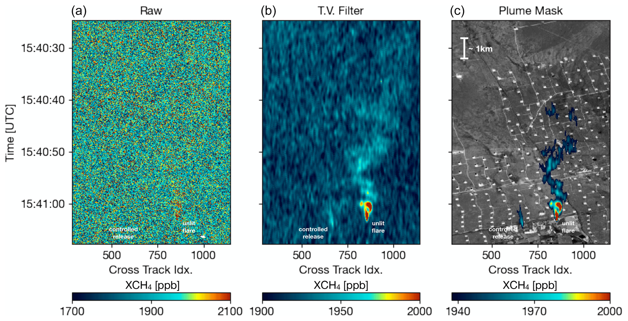
Figure 15Example plume mask applied to MethaneAIR data over the controlled-release site during RF04. Panels (a) and (b) show the MethaneAIR XCH4 retrievals obtained before and after the Chambolle TV filter was applied. Panel (c) shows the masked XCH4 overlaid on top of a grayscale image derived from the MethaneAIR radiance at 1622 nm. The plume mask detects the ∼ 100 kg h−1 plume at the controlled-release site as well as a much larger ∼ 1000 kg h−1 emission from an unlit flare near the release site.
The masking algorithm detects emissions from the flare up to 5 km downwind. While this shows that the retrieval performs well, it presents a conundrum: instruments like AVIRIS-NG (Thorpe et al., 2016) have high XCH4 detection limits but a very fine spatial resolution, which enables the detection of compact plumes close to the source. For MethaneAIR, the XCH4 plume gradients are smeared out near the source but remain detectable over large distances downwind. Thus, for retrievals over complex emission fields, multiple plumes may overlap, complicating point-source inversions.
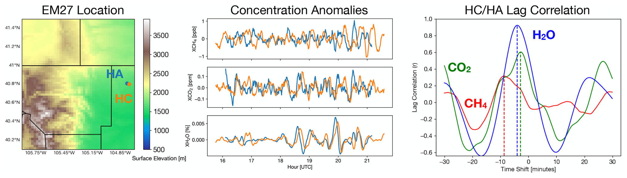
Figure 16The left-hand panel shows the location of the two EM27/SUN spectrometers (HA and HC) used in the winter campaign, overlaid on top of a GMTED2010 digital elevation map (Danielson and Gesch, 2011). The middle panel shows anomalies in dry-air mole fraction for CH4, CO2, and H2O measured by the two EM27/SUN instruments (HA and HC) during RF01 (8 November 2019). HC was located approximately 1 km downwind of HA (see main text). The anomalies were derived by subtracting data smoothed using a 1 h moving window from data smoothed with a 5 min boxcar running window. The right-hand panel shows the correlation between the anomaly time series for different time shifts relative to the HC time grid for the segment of HA between 18:00–20:00 UTC.
The plume mask's 2σ XCH4 thresholds, derived from real data (such as those illustrated in Fig. 15), tend to be up to 30 % higher (∼ 1.4 ppb) than those derived from the plume-free synthetic noisy retrievals. While a portion of this discrepancy may be explained by unidentified retrieval biases, meteorological drivers may also play an important role. For instance, the XCH4 retrievals from the EM27/SUN spectrometers collected during the winter campaign over a relatively clean background region show amplitude oscillations of ∼ 1 ppb (Fig. 16). In this case, the two sites were separated zonally by ∼ 1 km, with prevailing westerly surface winds. From the EM27 data, the XCH4 lag correlation peaks at 6 min, and similar values are observed for H2O and CO2. Such correlations are consistent with the eastward propagation of gravity waves driven by orographic forcing from the mountains to the west of the sites, which could generate XCH4 anomalies by varying the height of the planetary boundary layer. Such meteorological sources of variability are expected to be even larger in regions like O&G basins, where they would be amplified by higher boundary-layer CH4 mole fractions.
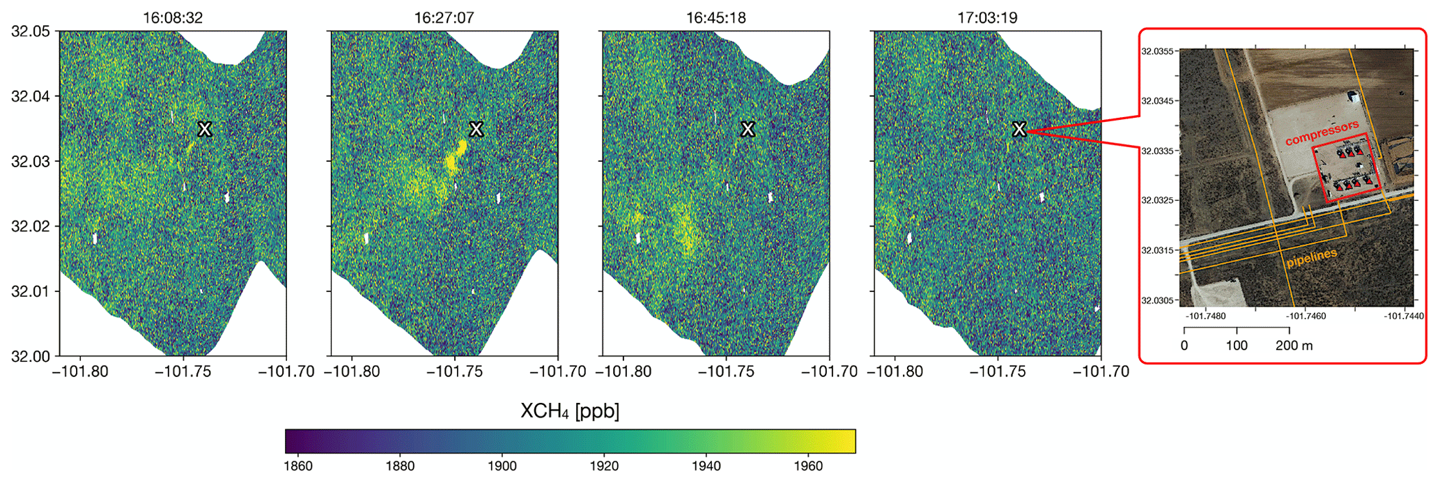
Figure 17XCH4 retrieved over an intermittent source (compressor station) during RF05 (3 August 2021). The title of each panel indicates the observation time in UTC, with the white “x” marking the source location. The rightmost panel shows a satellite image of the compressor station (© Google Earth), overlaid with the locations of pipelines (orange lines) and compressors (red triangles) from the Oil and Gas Infrastructure Mapping (OGIM) database (Omara et al., 2023).
Another source of higher XCH4 variability in the actual MethaneAIR data could be short-timescale emission variations, as supported by observations. Figure 17 shows one such example from RF05, where a plume emanating from a compressor station was observed on the approach to the controlled-release site at regular (∼ 18 min) intervals. In this instance, a large flash release was observed during the second overpass. Although the flash release had ceased by the third overpass, remnants of the initial plume were clearly detectable multiple kilometers downwind of the compressor station. Without the context of the earlier observation, these pulse releases can be challenging to interpret, and they represent a real source of variation in the data. We identified similar plumes that were not immediately adjacent to O&G infrastructure during the flights mapping the Permian Basin, suggesting that source intermittency at timescales of less than 1 h is common and highlighting that these plumes must be considered in the emission inversion of MethaneAIR and MethaneSAT data. We can see here that these plumes are observable by MethaneAIR and should be detectable by MethaneSAT, given the size of the observed enhancement and the spatial resolution and precision of both sensors.
6.3 Estimation of MethaneAIR's point-source detection limit
Now that we have characterized the instrument's performance and defined a plume detection method, the point-source detection limit for MethaneAIR can be estimated. To do so, we use a WRF-LES for the meteorological conditions of the controlled release for RF04 (Fig. 15), used for the IME calculations. The simulation was performed at a 100 × 100 m2 spatial resolution over a 5.6 × 5.6 km2 domain and then interpolated to the 5 × 1 pixel resolution (∼ 20×20 m2). Note that the lower resolution of the simulation may lead to an overly pessimistic estimate of the detection limit. We allow the simulation to spin up for 3 h and then simulate the transport of five point sources within the domain for the next 4 h. The mean wind speed during this period was 2.4 m s−1. The simulated XCH4 fields were saved every minute, yielding 1200 plume samples.
A simple estimate of the detection limit can be determined by scaling each plume sample to the minimum criteria that would allow it to be flagged by the plume-masking algorithm. From this, we determined a median point-source emission rate of 93 kg h−1 (interquartile range: 81–109 kg h−1) for the retrieval using 5 × 1 aggregated pixels, employing thresholds corresponding to a TV smoothing parameter λ value of 75. As previously discussed, natural atmospheric variability that is not due to the plume likely increases the background XCH4 threshold. If we assume that the 30 % higher threshold found for the real RF04 case is representative, then the median detection limit becomes 121 kg h−1 (interquartile range: 106–141 kg h−1). This simple bottom-up estimate of the detection limit is consistent with the 200 kg h−1 quantification limit we independently determined by assessing the performance of the IME method against the controlled-release experiments from RF04 and RF05 (Chulakadaba et al., 2023). The difference arises partly because here we are referring to detection rather than quantification and partly due to differences in the plume-masking approach used in Chulakadaba et al. (2023).
In order to estimate the accuracy of a point-source emission inversion using the MethaneAIR data, a full-circle OSSE (observing system simulation experiment) is required. In this experiment, synthetic MethaneAIR retrievals are created using a WRF-LES and then inverted via the IME method. Varon et al. (2018) performed a comprehensive set of OSSEs for a 50 × 50 m2 resolution instrument at various precision levels. At this coarser spatial resolution, the precision of MethaneAIR corresponds approximately to their 1 % precision case, which yielded an emission uncertainty of 70 kg h−1 + 5 % of the IME emission estimate. Note that there is additional uncertainty due to the use of a reanalysis wind product for estimating ueff, which was estimated to be 15 %–50 % depending on the wind speed. Overall, this suggests that MethaneAIR is capable of detecting 75 % of US O&G CH4 emissions as point sources, based on estimates from the US Greenhouse Gas Reporting Program (GHGRP) (Jacob et al., 2016; Varon et al., 2018). While there is considerable uncertainty in the GHGRP estimates, the point-source detection rate can be derived from the MethaneAIR data alone as it can also be used to constrain total basin emissions via flux inversions.
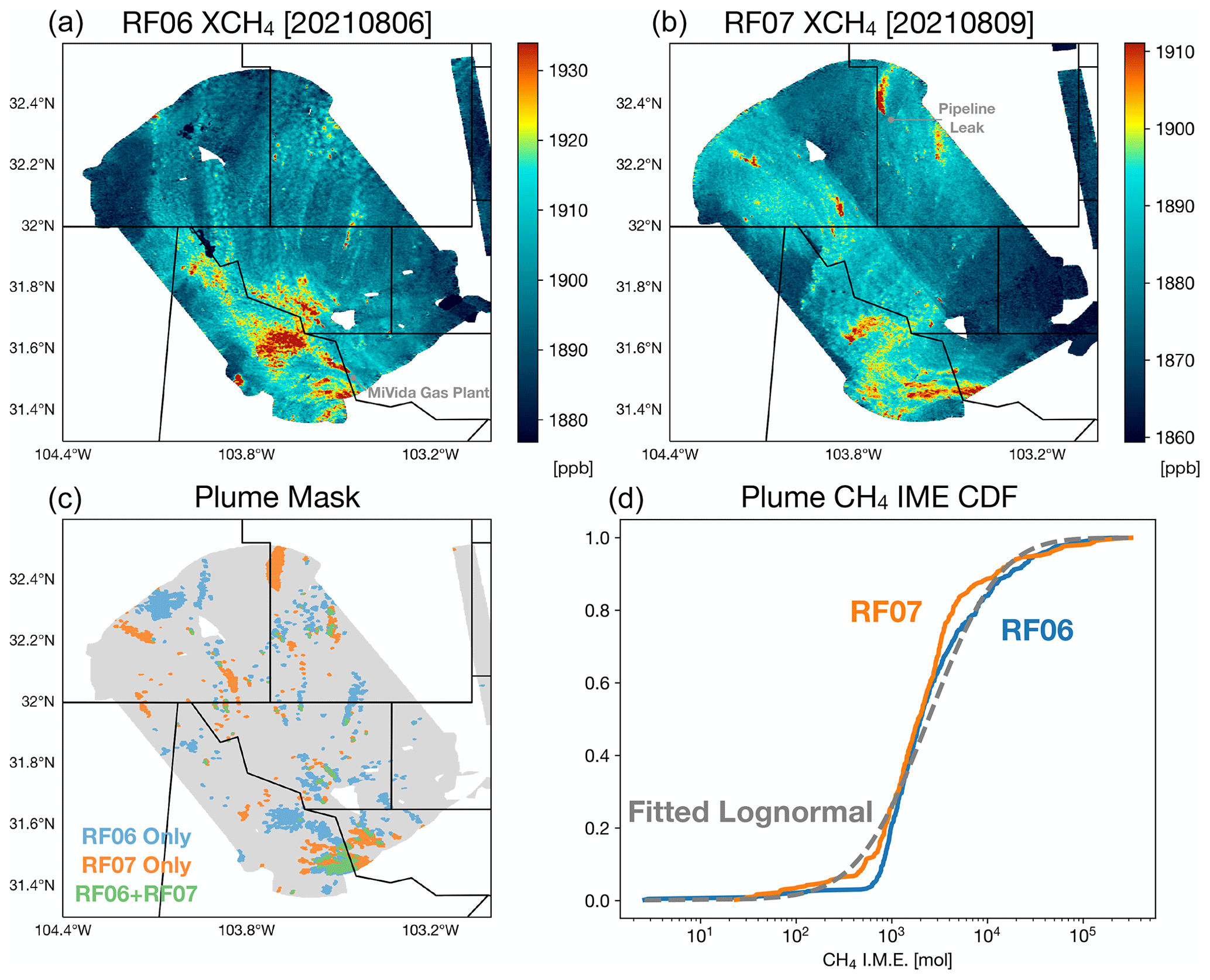
Figure 18Retrievals of XCH4 over the Delaware basin from two successive research flights. Panels (a) and (b) show gridded XCH4 at a 15 m spatial resolution. Panel (c) shows the gridded plume masks from both flights, using the algorithm described in Sect. 6, with regions detected by one or both flights indicated in different colors. Panel (d) shows the cumulative distribution of the IMEs derived from the plume masks for both flights.
Here, we present a case study typical of the flights. Figure 18 shows retrievals obtained over the O&G infrastructure of the Delaware sub-basin, located in the larger Permian Basin, during RF06 and RF07 (6 and 9 August 2021). As the flights were 3 d apart, this provides an opportunity to observe the spatial and temporal variability in sources over a major production region. The flight pattern was the same for both days, with the plane approaching from the north of the basin before repeating a clockwise oval pattern over the basin that gradually translated northeast with each loop (see the bottom-right panel of Fig. 1). For both days, the basin was mapped over a ∼ 2 h period between 10:00–12:00 local time (LT). The transport patterns for both days are evident from the plumes in the retrieved XCH4 maps, showing a generally southeasterly direction for RF06 and a southwesterly direction for RF07. During RF06, emissions were clustered around the southern part of the basin, whereas RF07 showed large sources to the north that were not present in RF06. In RF07, there was an increase in the XCH4 background over the course of the monitoring period, evidenced by the discontinuity in XCH4 along the line oriented northwest to southeast through the center of the image.
The sources identified during both flights are shown in the plume mask, verifying that the detected emitters in the basin are highly variable in space and time. The cumulative distribution function for the IMEs from both the flights is also shown in Fig. 18 and is heavily tailed, as seen in many previous studies (Zavala-Araiza et al., 2015; Brandt et al., 2016; Frankenberg et al., 2016; Cusworth et al., 2021). Despite the spatiotemporal sources differing in RF06 and RF07, their basin-wide point-source probability distributions are similar. If mean basin-wide emissions remain steadier over time, this could allow for a reduction in the frequency of target monitoring by MethaneSAT, enabling an expansion of the operational list of targets flagged for regular monitoring.
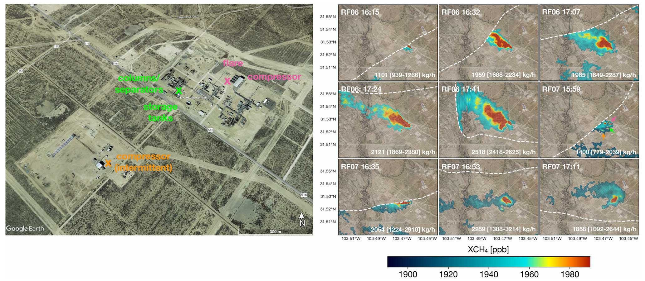
Figure 19XCH4 retrievals from repeated overpasses of the MiVida gas processing plant during RF06 and RF07. The left-hand panel shows a © Google Earth image of the plant, with the approximate locations of the three sources contributing to the observed plume within the plant indicated based on the XCH4 retrievals. The main infrastructure and potentially significant emissions are also labeled. The observed XCH4 plumes from each overpass are shown in the right-hand panel, with color-coded infrastructure locations indicated by arrows in the “RF07 15:59” plot. The observation times are given in UTC. Dashed lines indicate the edge of the aircraft swath. Emission rates computed using the IME method (Chulakadaba et al., 2023) are also indicated, along with the 2.5–97.5 percentile confidence interval (in square brackets). The IME method currently does not account for the impact of partially observed plumes, which may lead to emission underestimates.
We now take a closer look at two of the largest emitters identified from the Delaware survey. First, we examine the MiVida gas processing plant, where we observed persistently large CH4 plumes for both flights. The plant is located at the southern end of the basin, as indicated in Fig. 18a. A total of nine overpasses were made, allowing for good characterization of the source (Fig. 19) using the IME method. The estimated emissions were persistent and large, ranging from 1858–2518 kg h−1, excluding emissions from the RF06 16:15 UTC and RF07 17:11 UTC overpasses due to poor observational coverage of the target site. According to Homeland Infrastructure Foundation-Level Data from the US Department of Homeland Security (DHS), approximately 190 million cubic feet per day (cfd; ∼ 5.4 million standard cubic meters per day) of gas is processed by the plant. With a reported CH4 mole fraction of 0.77 (US EPA Greenhouse Gas Reporting Program; GHGRP, 2024), this implies a leak rate of 1.6 %–2.1 %. This rate is higher than any rates observed from a comprehensive survey of gas plants (Marchese et al., 2015) and thus suggests a large source of unintended emissions at the plant. From the observed plumes, we identified three source locations, as indicated in the left panel of Fig. 19. The largest contributor, indicated by the pink cross, is close to a flare stack and compressor engine shed. The CH4 values reported to the EPA GHGRP from the flares correspond to about half of the observed emissions (1121 kg h−1), indicating that there are other large sources within the plant. There is also a contribution from a set of condensate storage tanks, absorption columns, and liquid–gas separators (green cross in the left panel of Fig. 19), clearly visible from the corresponding XCH4 enhancement seen in the first pass of RF06. This is consistent with previous surveys of O&G gathering and processing facilities, which observed that venting from tanks tends to be an important source for high-emitting sites (Mitchell et al., 2015; Lyon et al., 2016). Finally, there is an intermittent source to the south of the plant, near another set of compressor engines, most clearly visible during the last three RF07 overpasses.
The second case described here occurred during RF07, in which a large plume extending over 20 km was observed at the northern edge of the Delaware basin (top-right corner of Fig. 20). The origin of the plume was located precisely over an O&G gathering pipeline. The IME-based emission estimate is ∼ 6100 kg h−1 (5700–6500 kg h−1; Chulakadaba et al., 2023), considerable for a single source. For comparison, Zhang et al. (2020) estimated Permian Basin emissions of ∼ 2.7 Tg a−1 from TROPOMI, meaning the pipeline leak corresponded to 2 % of the average annual emissions from the entire basin. On 24 August, 15 d after RF07, the pipeline operator filed an incident report (Lucid Energy Delaware, 2021) about a rupture along a pipeline weld caused by high line pressure. Based on the operator's report on the volume and duration of natural gas vented, we estimated a methane emission rate of 8200 kg h−1, which is consistent in terms of magnitude with that observed by MethaneAIR. This case demonstrates that even large-magnitude leaks can go undetected for long periods of time. It also suggests that through regular O&G basin monitoring, MethaneSAT will be an important addition to the existing network of satellites capable of detecting large methane leaks (Irakulis-Loitxate et al., 2022) and will contribute to the mitigation of methane leaks through international activities, such as the Methane Alert and Response System (UNEP, 2023).
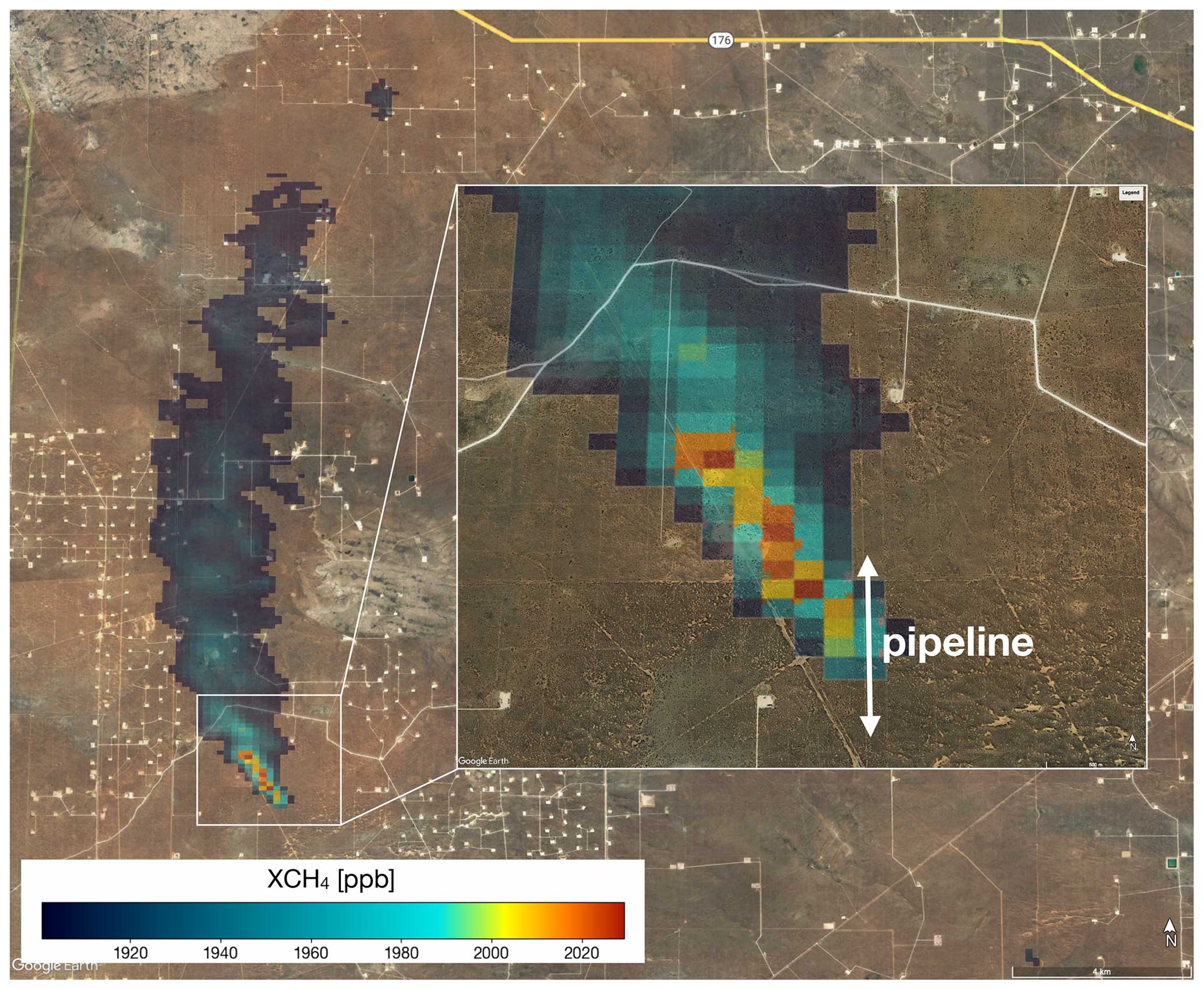
Figure 20Retrieval of a large plume caused by a pipeline leak during RF07, gridded at a 100×100 m2 resolution and overlaid on top of © Google Earth imagery.
Here, we have described the XCH4 retrieval algorithm designated for MethaneSAT, based on the CO2 proxy retrieval approach, and applied it to observations from the first campaign of MethaneAIR, an airborne spectrometer with specifications similar to those of the future satellite.
Analysis of the flight observations revealed temperature-induced drifts in instrument focus over the course of the flight, typically changing ISRF widths by 10 %–30 %. We show that these drifts can be mostly corrected by fitting a squeeze factor to the tabulated ISRF. We present a PLS-regression-based method for removing cross-track biases induced by imperfect modeling of the ISRF defocus using the retrieved squeeze factors. Subsequent validation against ground-based EM27/SUN and TROPOMI retrievals shows that the instrument's accuracy is typically within ∼ 1 %.
Based on the flight retrievals, we find that the instrument's precision is typically around 35 ppb (∼ 1.9 %) per 20×20 m2 pixel (5×1 aggregated pixels). We estimate that this translates to a median point-source detection limit of 121 kg h−1 for sufficiently bright (albedo > ∼ 0.15) cloud-free scenes, which aligns with the 200 kg h−1 quantification limit determined by Chulakadaba et al. (2023).
Importantly, we find no strong dependence on surface reflectance in the MethaneAIR results. This was a key untested assumption in the early emission inversion OSSEs used to inform the MethaneSAT instrument requirements (Benmergui, 2019). In those original experiments, the assumed precision of MethaneSAT was 0.15 % at a 1×1 km2 resolution. In follow-up experiments, it was found that the satellite could meet its emission constraint goals with this level of precision at a scale of 5×5 km2. We expect MethaneSAT to have a precision per pixel similar to that of MethaneAIR (35 ppb; Sect. S2.1). At these levels, the 0.15 % target precision will be achieved at a scale of ∼ 3×3 km2, well within the precision requirement6. Although the instruments have different spatial resolutions, we do not find large differences in cloud contamination (Sect. S2.3.1) or in biases caused by subpixel inhomogeneities in illumination (Sect. S2.3.2) or methane concentration (Sect. S2.3.3) between the two instruments.
The pixel precision–accuracy combination demonstrated here also highlights MethaneAIR's uniqueness among current aircraft sensors, which are capable of making retrievals with a TROPOMI-like precision and accuracy at scales of ∼ 100×100 m2. At these scales, new features, such as disconnected CH4 plumes from intermittent sources and XCH4 gradients driven by diffuse sources and boundary layer structures, become measurable. As such, MethaneAIR provides a valuable test bed for developing new emission inversion approaches that account for these observable features prior to MethaneSAT's launch.
The Level-2 (L2) retrieval code is available upon request. L2 data are available through the NCAR/University Corporation for Atmospheric Research (UCAR) Earth Observing Laboratory (EOL) data archive at https://doi.org/10.26023/J2CB-E2RX-J700 (Chan Miller et al., 2023). The GGG2020 software package used to generate the a priori trace gas profiles and spectroscopic line lists for calculating CO2, H2O, and CH4 are available through the Caltech data repository (https://doi.org/10.22002/D1.8974, Laughner et al., 2022; https://doi.org/10.14291/TCCON.GGG2020.ATMNV.R0, Toon, 2022a; https://doi.org/10.14291/TCCON.GGG2020.ATM.R0, Toon, 2022b).
The supplement related to this article is available online at: https://doi.org/10.5194/amt-17-5429-2024-supplement.
CCM led the study, developed the retrieval algorithm, and wrote the paper, incorporating comments and revisions from all authors. SR and JSW contributed to the L2 algorithm development and data analysis. SCW, KC, XL, KS, JSB, JEF, YL, MS, and CCM contributed to the mission design, including flight planning and instrument requirements. BCD integrated the instrument into the aircraft. JS, JEF, and JH performed the calibration measurements and conducted the instrument flights. EC, BL, AHS, KS, and CS developed the L1 calibration algorithms. AC, MS, and JSB conducted MethaneAIR CH4 emission inversions. JLL developed the GGG2020's a priori profile software that was used by the L2 algorithm. JEF and BCB deployed the EM27/SUN instruments. RG and MO provided facility-level bottom-up CH4 estimates.
The contact author has declared that none of the authors has any competing interests.
Publisher’s note: Copernicus Publications remains neutral with regard to jurisdictional claims made in the text, published maps, institutional affiliations, or any other geographical representation in this paper. While Copernicus Publications makes every effort to include appropriate place names, the final responsibility lies with the authors.
The Environmental Defense Fund provides primary support for the MethaneAIR and MethaneSAT projects to Harvard University, the Harvard–Smithsonian Center for Astrophysics, and the University at Buffalo. We gratefully acknowledge assistance from the NSF EAGER grant awarded to Harvard University (grant no. 1856426), which supported the flight campaign. Joshua L. Laughner was supported by the National Aeronautics and Space Administration (NASA; grant no. NNX17AE15G), with research carried out at the Jet Propulsion Laboratory, California Institute of Technology, under a contract with NASA (contract no. 80NM0018D0004). Bianca C. Baier was supported in part by NASA (grant no. 80NSSC18K0898), a NOAA cooperative agreement (grant no. NA22OAR4320151), and a NASA–JPL subaward (grant no. 1615988). We would like to acknowledge the technical support from Philip Handley, Timothy Newberger, and Anna McAuliffe regarding the EM27/SUN observations collected at NOAA ESRL, and we would like to thank Frank Hase for loaning the spectrometer. Finally, we extend our appreciation to the MethaneSAT software team (Nick LoFaso, Chris Hairfield, and Sasha Ayvazov), who adapted the retrieval presented here to a cloud environment for future MethaneAIR campaigns.
This research has been supported by the National Science Foundation as part of the EAGER (grant no. 1856426), the Environmental Defense Fund, the National Aeronautics and Space Administration (NASA; grant nos. NNX17AE15G, 80NM0018D0004, 80NSSC18K0898, and 1615988), and a NOAA cooperative agreement (grant no. NA22OAR4320151).
This paper was edited by Dominik Brunner and reviewed by Jakob Borchardt and Philipp Hochstaffl.
Aben, I., Hasekamp, O., and Hartmann, W.: Uncertainties in the space-based measurements of CO2 columns due to scattering in the Earth's atmosphere, J. Quant. Spectrosc. Ra., 104, 450–459, https://doi.org/10.1016/j.jqsrt.2006.09.013, 2007. a
Alberti, C., Hase, F., Frey, M., Dubravica, D., Blumenstock, T., Dehn, A., Castracane, P., Surawicz, G., Harig, R., Baier, B. C., Bès, C., Bi, J., Boesch, H., Butz, A., Cai, Z., Chen, J., Crowell, S. M., Deutscher, N. M., Ene, D., Franklin, J. E., García, O., Griffith, D., Grouiez, B., Grutter, M., Hamdouni, A., Houweling, S., Humpage, N., Jacobs, N., Jeong, S., Joly, L., Jones, N. B., Jouglet, D., Kivi, R., Kleinschek, R., Lopez, M., Medeiros, D. J., Morino, I., Mostafavipak, N., Müller, A., Ohyama, H., Palmer, P. I., Pathakoti, M., Pollard, D. F., Raffalski, U., Ramonet, M., Ramsay, R., Sha, M. K., Shiomi, K., Simpson, W., Stremme, W., Sun, Y., Tanimoto, H., Té, Y., Tsidu, G. M., Velazco, V. A., Vogel, F., Watanabe, M., Wei, C., Wunch, D., Yamasoe, M., Zhang, L., and Orphal, J.: Improved calibration procedures for the EM27/SUN spectrometers of the COllaborative Carbon Column Observing Network (COCCON), Atmos. Meas. Tech., 15, 2433–2463, https://doi.org/10.5194/amt-15-2433-2022, 2022. a, b
Benmergui, J.: Innovations in Modeling and Statistical Analysis for Greenhouse Gas Flux Monitoring, PhD Thesis, Harvard University, https://www.semanticscholar.org/paper/Innovations-in-Modeling-and-Statistical-Analysis-Benmergui/8f46f431006ad3c71c82efe2e3089f261abffe35 (last access: 30 August 2024), 2019. a, b
Boersma, K. F., Eskes, H. J., Dirksen, R. J., van der A, R. J., Veefkind, J. P., Stammes, P., Huijnen, V., Kleipool, Q. L., Sneep, M., Claas, J., Leitão, J., Richter, A., Zhou, Y., and Brunner, D.: An improved tropospheric NO2 column retrieval algorithm for the Ozone Monitoring Instrument, Atmos. Meas. Tech., 4, 1905–1928, https://doi.org/10.5194/amt-4-1905-2011, 2011. a
Borsdorff, T., aan de Brugh, J., Schneider, A., Lorente, A., Birk, M., Wagner, G., Kivi, R., Hase, F., Feist, D. G., Sussmann, R., Rettinger, M., Wunch, D., Warneke, T., and Landgraf, J.: Improving the TROPOMI CO data product: update of the spectroscopic database and destriping of single orbits, Atmos. Meas. Tech., 12, 5443–5455, https://doi.org/10.5194/amt-12-5443-2019, 2019. a
Brandt, A. R., Heath, G. A., and Cooley, D.: Methane Leaks from Natural Gas Systems Follow Extreme Distributions, Environ. Sci. Technol., 50, 12512–12520, https://doi.org/10.1021/acs.est.6b04303, 2016. a, b
Butz, A., Hasekamp, O. P., Frankenberg, C., Vidot, J., and Aben, I.: CH4 retrievals from space-based solar backscatter measurements: Performance evaluation against simulated aerosol and cirrus loaded scenes, J. Geophys. Res.-Atmos., 115, D24302, https://doi.org/10.1029/2010JD014514, 2010. a, b
Carbon Mapper, Inc.: Carbon Mapper: Our Mission – Technology, https://carbonmapper.org/articles/tanager-methane-performance-specifications (last access: 30 August 2024), 2023. a
Chambolle, A.: An Algorithm for Total Variation Minimization and Applications, J. Math. Imaging Vis., 20, 89–97, https://doi.org/10.1023/B:JMIV.0000011325.36760.1e, 2004. a
Chan Miller, C., Franklin, J. E., Roche, S., Wilzewski, J. S., Sun, K., Liu, X., Chance, K., Souri, A. H., Conway, E., Samra, J., Hawthorne, J., Staebell, C., Chulakadabba, A., Sargent, M., Benmergui, J. S., Daube, B. C., Li, Y., Laughner, J., and Wofsy, S. C.: MethaneAIR: Airborne Imaging Spectrometer Level 2 Ungridded Data, NCAR UCAR EOL data archive [data set], https://doi.org/10.26023/J2CB-E2RX-J700, 2023. a
Chulakadabba, A., Sargent, M., Lauvaux, T., Benmergui, J. S., Franklin, J. E., Chan Miller, C., Wilzewski, J. S., Roche, S., Conway, E., Souri, A. H., Sun, K., Luo, B., Hawthrone, J., Samra, J., Daube, B. C., Liu, X., Chance, K., Li, Y., Gautam, R., Omara, M., Rutherford, J. S., Sherwin, E. D., Brandt, A., and Wofsy, S. C.: Methane point source quantification using MethaneAIR: a new airborne imaging spectrometer, Atmos. Meas. Tech., 16, 5771–5785, https://doi.org/10.5194/amt-16-5771-2023, 2023. a, b, c, d, e, f, g, h
Conway, E. K., Souri, A. H., Benmergui, J., Sun, K., Liu, X., Staebell, C., Chan Miller, C., Franklin, J., Samra, J., Wilzewski, J., Roche, S., Luo, B., Chulakadabba, A., Sargent, M., Hohl, J., Daube, B., Gordon, I., Chance, K., and Wofsy, S.: Level0 to Level1B processor for MethaneAIR, Atmos. Meas. Tech., 17, 1347–1362, https://doi.org/10.5194/amt-17-1347-2024, 2024. a
Cusworth, D. H., Duren, R. M., Thorpe, A. K., Olson-Duvall, W., Heckler, J., Chapman, J. W., Eastwood, M. L., Helmlinger, M. C., Green, R. O., Asner, G. P., Dennison, P. E., and Miller, C. E.: Intermittency of Large Methane Emitters in the Permian Basin, Environ. Sci. Technol. Lett., 8, 567–573, https://doi.org/10.1021/acs.estlett.1c00173, 2021. a, b
Cusworth, D. H., Thorpe, A. K., Ayasse, A. K., Stepp, D., Heckler, J., Asner, G. P., Miller, C. E., Yadav, V., Chapman, J. W., Eastwood, M. L., Green, R. O., Hmiel, B., Lyon, D. R., and Duren, R. M.: Strong methane point sources contribute a disproportionate fraction of total emissions across multiple basins in the United States, P. Natl. Acad. Sci. USA, 119, e2202338119, https://doi.org/10.1073/pnas.2202338119, 2022. a
Danielson, J. J. and Gesch, D. B.: Global Multi-resolution Terrain Elevation Data 2010 (GMTED2010), U.S Geological Survey Open-File Report, 2011-1073, 26 pp., https://doi.org/10.3133/ofr20111073, 2011. a
Deng, Z., Ciais, P., Tzompa-Sosa, Z. A., Saunois, M., Qiu, C., Tan, C., Sun, T., Ke, P., Cui, Y., Tanaka, K., Lin, X., Thompson, R. L., Tian, H., Yao, Y., Huang, Y., Lauerwald, R., Jain, A. K., Xu, X., Bastos, A., Sitch, S., Palmer, P. I., Lauvaux, T., d'Aspremont, A., Giron, C., Benoit, A., Poulter, B., Chang, J., Petrescu, A. M. R., Davis, S. J., Liu, Z., Grassi, G., Albergel, C., Tubiello, F. N., Perugini, L., Peters, W., and Chevallier, F.: Comparing national greenhouse gas budgets reported in UNFCCC inventories against atmospheric inversions, Earth Syst. Sci. Data, 14, 1639–1675, https://doi.org/10.5194/essd-14-1639-2022, 2022. a
Etminan, M., Myhre, G., Highwood, E. J., and Shine, K. P.: Radiative forcing of carbon dioxide, methane, and nitrous oxide: A significant revision of the methane radiative forcing, Geophys. Res. Lett., 43, 12614–12623, https://doi.org/10.1002/2016GL071930, 2016. a
Frankenberg, C., Platt, U., and Wagner, T.: Iterative maximum a posteriori (IMAP)-DOAS for retrieval of strongly absorbing trace gases: Model studies for CH4 and CO2 retrieval from near infrared spectra of SCIAMACHY onboard ENVISAT, Atmos. Chem. Phys., 5, 9–22, https://doi.org/10.5194/acp-5-9-2005, 2005. a, b
Frankenberg, C., Meirink, J. F., Bergamaschi, P., Goede, A. P. H., Heimann, M., Körner, S., Platt, U., van Weele, M., and Wagner, T.: Satellite chartography of atmospheric methane from SCIAMACHY on board ENVISAT: Analysis of the years 2003 and 2004, J. Geophys. Res.-Atmos., 111, D07303, https://doi.org/10.1029/2005JD006235, 2006. a, b
Frankenberg, C., Thorpe, A. K., Thompson, D. R., Hulley, G., Kort, E. A., Vance, N., Borchardt, J., Krings, T., Gerilowski, K., Sweeney, C., Conley, S., Bue, B. D., Aubrey, A. D., Hook, S., and Green, R. O.: Airborne methane remote measurements reveal heavy-tail flux distribution in Four Corners region, P. Natl. Acad. Sci. USA, 113, 9734–9739, https://doi.org/10.1073/pnas.1605617113, 2016. a, b, c
Frey, M., Sha, M. K., Hase, F., Kiel, M., Blumenstock, T., Harig, R., Surawicz, G., Deutscher, N. M., Shiomi, K., Franklin, J. E., Bösch, H., Chen, J., Grutter, M., Ohyama, H., Sun, Y., Butz, A., Mengistu Tsidu, G., Ene, D., Wunch, D., Cao, Z., Garcia, O., Ramonet, M., Vogel, F., and Orphal, J.: Building the COllaborative Carbon Column Observing Network (COCCON): long-term stability and ensemble performance of the EM27/SUN Fourier transform spectrometer, Atmos. Meas. Tech., 12, 1513–1530, https://doi.org/10.5194/amt-12-1513-2019, 2019. a
Geibel, M. C., Messerschmidt, J., Gerbig, C., Blumenstock, T., Chen, H., Hase, F., Kolle, O., Lavrič, J. V., Notholt, J., Palm, M., Rettinger, M., Schmidt, M., Sussmann, R., Warneke, T., and Feist, D. G.: Calibration of column-averaged CH4 over European TCCON FTS sites with airborne in-situ measurements, Atmos. Chem. Phys., 12, 8763–8775, https://doi.org/10.5194/acp-12-8763-2012, 2012. a
Gerilowski, K., Tretner, A., Krings, T., Buchwitz, M., Bertagnolio, P. P., Belemezov, F., Erzinger, J., Burrows, J. P., and Bovensmann, H.: MAMAP – a new spectrometer system for column-averaged methane and carbon dioxide observations from aircraft: instrument description and performance analysis, Atmos. Meas. Tech., 4, 215–243, https://doi.org/10.5194/amt-4-215-2011, 2011. a
GHGRP: U.S. EPA Greenhouse Gas Reporting Program (GHGRP), https://www.epa.gov/ghgreporting, last access: 30 August 2024. a
Gisi, M., Hase, F., Dohe, S., Blumenstock, T., Simon, A., and Keens, A.: XCO2-measurements with a tabletop FTS using solar absorption spectroscopy, Atmos. Meas. Tech., 5, 2969–2980, https://doi.org/10.5194/amt-5-2969-2012, 2012. a
Guanter, L., Irakulis-Loitxate, I., Gorroño, J., Sánchez-García, E., Cusworth, D. H., Varon, D. J., Cogliati, S., and Colombo, R.: Mapping methane point emissions with the PRISMA spaceborne imaging spectrometer, Remote Sens. Environ., 265, 112671, https://doi.org/10.1016/j.rse.2021.112671, 2021. a
Guerlet, S., Butz, A., Schepers, D., Basu, S., Hasekamp, O. P., Kuze, A., Yokota, T., Blavier, J.-F., Deutscher, N. M., Griffith, D. W. T., Hase, F., Kyro, E., Morino, I., Sherlock, V., Sussmann, R., Galli, A., and Aben, I.: Impact of aerosol and thin cirrus on retrieving and validating XCO2 from GOSAT shortwave infrared measurements, J. Geophys. Res.-Atmos., 118, 4887–4905, https://doi.org/10.1002/jgrd.50332, 2013. a
Hansen, P. C.: The L-curve and its use in the numerical treatment of inverse problems, Computational Inverse Problems in Electrocardiology, WIT Press, 119–142, ISBN 978-1-85312-614-7, 2000. a
Heidinger, A. K., Evan, A. T., Foster, M. J., and Walther, A.: A Naive Bayesian Cloud-Detection Scheme Derived from CALIPSO and Applied within PATMOS-x, J. Appl. Meteorol. Clim., 51, 1129–1144, https://doi.org/10.1175/JAMC-D-11-02.1, 2012. a
Hochstaffl, P., Schreier, F., Köhler, C. H., Baumgartner, A., and Cerra, D.: Methane retrievals from airborne HySpex observations in the shortwave infrared, Atmos. Meas. Tech., 16, 4195–4214, https://doi.org/10.5194/amt-16-4195-2023, 2023. a
Hu, H., Landgraf, J., Detmers, R., Borsdorff, T., Aan de Brugh, J., Aben, I., Butz, A., and Hasekamp, O.: Toward Global Mapping of Methane With TROPOMI: First Results and Intersatellite Comparison to GOSAT, Geophys. Res. Lett., 45, 3682–3689, https://doi.org/10.1002/2018GL077259, 2018. a, b, c, d
Irakulis-Loitxate, I., Guanter, L., Maasakkers, J. D., Zavala-Araiza, D., and Aben, I.: Satellites Detect Abatable Super-Emissions in One of the World's Largest Methane Hotspot Regions, Environ. Sci. Technol., 56, 2143–2152, https://doi.org/10.1021/acs.est.1c04873, 2022. a
Jacob, D. J., Turner, A. J., Maasakkers, J. D., Sheng, J., Sun, K., Liu, X., Chance, K., Aben, I., McKeever, J., and Frankenberg, C.: Satellite observations of atmospheric methane and their value for quantifying methane emissions, Atmos. Chem. Phys., 16, 14371–14396, https://doi.org/10.5194/acp-16-14371-2016, 2016. a
Jacob, D. J., Varon, D. J., Cusworth, D. H., Dennison, P. E., Frankenberg, C., Gautam, R., Guanter, L., Kelley, J., McKeever, J., Ott, L. E., Poulter, B., Qu, Z., Thorpe, A. K., Worden, J. R., and Duren, R. M.: Quantifying methane emissions from the global scale down to point sources using satellite observations of atmospheric methane, Atmos. Chem. Phys., 22, 9617–9646, https://doi.org/10.5194/acp-22-9617-2022, 2022. a, b, c
Janardanan, R., Maksyutov, S., Tsuruta, A., Wang, F., Tiwari, Y. K., Valsala, V., Ito, A., Yoshida, Y., Kaiser, J. W., Janssens-Maenhout, G., Arshinov, M., Sasakawa, M., Tohjima, Y., Worthy, D. E. J., Dlugokencky, E. J., Ramonet, M., Arduini, J., Lavric, J. V., Piacentino, S., Krummel, P. B., Langenfelds, R. L., Mammarella, I., and Matsunaga, T.: Country-Scale Analysis of Methane Emissions with a High-Resolution Inverse Model Using GOSAT and Surface Observations, Remote Sens., 12, 375, https://doi.org/10.3390/rs12030375, 2020. a
Jervis, D., McKeever, J., Durak, B. O. A., Sloan, J. J., Gains, D., Varon, D. J., Ramier, A., Strupler, M., and Tarrant, E.: The GHGSat-D imaging spectrometer, Atmos. Meas. Tech., 14, 2127–2140, https://doi.org/10.5194/amt-14-2127-2021, 2021. a
Karion, A., Sweeney, C., Tans, P., and Newberger, T.: AirCore: An Innovative Atmospheric Sampling System, J. Atmos. Ocean. Tech., 27, 1839–1853, https://doi.org/10.1175/2010JTECHA1448.1, 2010. a
Krautwurst, S., Gerilowski, K., Jonsson, H. H., Thompson, D. R., Kolyer, R. W., Iraci, L. T., Thorpe, A. K., Horstjann, M., Eastwood, M., Leifer, I., Vigil, S. A., Krings, T., Borchardt, J., Buchwitz, M., Fladeland, M. M., Burrows, J. P., and Bovensmann, H.: Methane emissions from a Californian landfill, determined from airborne remote sensing and in situ measurements, Atmos. Meas. Tech., 10, 3429–3452, https://doi.org/10.5194/amt-10-3429-2017, 2017. a
Krings, T., Gerilowski, K., Buchwitz, M., Reuter, M., Tretner, A., Erzinger, J., Heinze, D., Pflüger, U., Burrows, J. P., and Bovensmann, H.: MAMAP – a new spectrometer system for column-averaged methane and carbon dioxide observations from aircraft: retrieval algorithm and first inversions for point source emission rates, Atmos. Meas. Tech., 4, 1735–1758, https://doi.org/10.5194/amt-4-1735-2011, 2011. a, b
Krings, T., Neininger, B., Gerilowski, K., Krautwurst, S., Buchwitz, M., Burrows, J. P., Lindemann, C., Ruhtz, T., Schüttemeyer, D., and Bovensmann, H.: Airborne remote sensing and in situ measurements of atmospheric CO2 to quantify point source emissions, Atmos. Meas. Tech., 11, 721–739, https://doi.org/10.5194/amt-11-721-2018, 2018. a
Larrick, G., Tian, Y., Rogers, U., Acosta, H., and Shen, F.: Interactive Visualization of 3D Terrain Data Stored in the Cloud, in: 2020 11th IEEE Annual Ubiquitous Computing, Electronics Mobile Communication Conference (UEMCON), 28–31 October 2020, New York, NY, USA, IEEE, 63–70, https://doi.org/10.1109/UEMCON51285.2020.9298063, 2020. a
Laughner, J., Andrews, A., Roche, S., Kiel, M., and Toon, G. C.: ginput v1.1.5: GGG2020 prior profile software, Medium: Gzipped tarball, California Institute of Technology Data Repository [code], https://doi.org/10.22002/D1.8974, 2022. a, b, c
Laughner, J. L., Roche, S., Kiel, M., Toon, G. C., Wunch, D., Baier, B. C., Biraud, S., Chen, H., Kivi, R., Laemmel, T., McKain, K., Quéhé, P.-Y., Rousogenous, C., Stephens, B. B., Walker, K., and Wennberg, P. O.: A new algorithm to generate a priori trace gas profiles for the GGG2020 retrieval algorithm, Atmos. Meas. Tech., 16, 1121–1146, https://doi.org/10.5194/amt-16-1121-2023, 2023. a, b
Laughner, J. L., Toon, G. C., Mendonca, J., Petri, C., Roche, S., Wunch, D., Blavier, J.-F., Griffith, D. W. T., Heikkinen, P., Keeling, R. F., Kiel, M., Kivi, R., Roehl, C. M., Stephens, B. B., Baier, B. C., Chen, H., Choi, Y., Deutscher, N. M., DiGangi, J. P., Gross, J., Herkommer, B., Jeseck, P., Laemmel, T., Lan, X., McGee, E., McKain, K., Miller, J., Morino, I., Notholt, J., Ohyama, H., Pollard, D. F., Rettinger, M., Riris, H., Rousogenous, C., Sha, M. K., Shiomi, K., Strong, K., Sussmann, R., Té, Y., Velazco, V. A., Wofsy, S. C., Zhou, M., and Wennberg, P. O.: The Total Carbon Column Observing Network's GGG2020 data version, Earth Syst. Sci. Data, 16, 2197–2260, https://doi.org/10.5194/essd-16-2197-2024, 2024. a
Liu, M., van der A, R., van Weele, M., Eskes, H., Lu, X., Veefkind, P., de Laat, J., Kong, H., Wang, J., Sun, J., Ding, J., Zhao, Y., and Weng, H.: A New Divergence Method to Quantify Methane Emissions Using Observations of Sentinel-5P TROPOMI, Geophys. Res. Lett., 48, e2021GL094151, https://doi.org/10.1029/2021GL094151, 2021. a, b
Lorente, A., Borsdorff, T., Butz, A., Hasekamp, O., aan de Brugh, J., Schneider, A., Wu, L., Hase, F., Kivi, R., Wunch, D., Pollard, D. F., Shiomi, K., Deutscher, N. M., Velazco, V. A., Roehl, C. M., Wennberg, P. O., Warneke, T., and Landgraf, J.: Methane retrieved from TROPOMI: improvement of the data product and validation of the first 2 years of measurements, Atmos. Meas. Tech., 14, 665–684, https://doi.org/10.5194/amt-14-665-2021, 2021. a, b, c
Lorente, A., Borsdorff, T., Martinez-Velarte, M. C., and Landgraf, J.: Accounting for surface reflectance spectral features in TROPOMI methane retrievals, Atmos. Meas. Tech., 16, 1597–1608, https://doi.org/10.5194/amt-16-1597-2023, 2023. a
Lu, X., Jacob, D. J., Zhang, Y., Maasakkers, J. D., Sulprizio, M. P., Shen, L., Qu, Z., Scarpelli, T. R., Nesser, H., Yantosca, R. M., Sheng, J., Andrews, A., Parker, R. J., Boesch, H., Bloom, A. A., and Ma, S.: Global methane budget and trend, 2010–2017: complementarity of inverse analyses using in situ (GLOBALVIEWplus CH4 ObsPack) and satellite (GOSAT) observations, Atmos. Chem. Phys., 21, 4637–4657, https://doi.org/10.5194/acp-21-4637-2021, 2021. a
Lucid Energy Delaware, LLC: Notification Of Release, 372422 (44680), New Mexico Energy, Minerals and Natural Resources Department, https://ocdimage.emnrd.nm.gov/imaging/IncidentFileView.aspx?incident=nAPP2123850791 (last access: 10 February 2022), 2021. a
Lyon, D. R., Alvarez, R. A., Zavala-Araiza, D., Brandt, A. R., Jackson, R. B., and Hamburg, S. P.: Aerial Surveys of Elevated Hydrocarbon Emissions from Oil and Gas Production Sites, Environ. Sci. Technol., 50, 4877–4886, https://doi.org/10.1021/acs.est.6b00705, 2016. a
Maasakkers, J. D., Jacob, D. J., Sulprizio, M. P., Scarpelli, T. R., Nesser, H., Sheng, J.-X., Zhang, Y., Hersher, M., Bloom, A. A., Bowman, K. W., Worden, J. R., Janssens-Maenhout, G., and Parker, R. J.: Global distribution of methane emissions, emission trends, and OH concentrations and trends inferred from an inversion of GOSAT satellite data for 2010–2015, Atmos. Chem. Phys., 19, 7859–7881, https://doi.org/10.5194/acp-19-7859-2019, 2019. a
Malley, C. S., Borgford-Parnell, N., Haeussling, S., Howard, I. C., Lefèvre, E. N., and Kuylenstierna, J. C. I.: A roadmap to achieve the global methane pledge, Environ. Res. Climate, 2, 011003, https://doi.org/10.1088/2752-5295/acb4b4, 2023. a
Marchese, A. J., Vaughn, T. L., Zimmerle, D. J., Martinez, D. M., Williams, L. L., Robinson, A. L., Mitchell, A. L., Subramanian, R., Tkacik, D. S., Roscioli, J. R., and Herndon, S. C.: Methane Emissions from United States Natural Gas Gathering and Processing, Environ. Sci. Technol., 49, 10718–10727, https://doi.org/10.1021/acs.est.5b02275, 2015. a
Mendonca, J., Strong, K., Toon, G. C., Wunch, D., Sung, K., Deutscher, N. M., Griffith, D. W. T., and Franklin, J. E.: Improving atmospheric CO2 retrievals using line mixing and speed-dependence when fitting high-resolution ground-based solar spectra, J. Mol. Spectrosc., 323, 15–27, https://doi.org/10.1016/j.jms.2016.01.007, 2016. a
Mendonca, J., Strong, K., Sung, K., Devi, V. M., Toon, G. C., Wunch, D., and Franklin, J. E.: Using high-resolution laboratory and ground-based solar spectra to assess CH4 absorption coefficient calculations, J. Quant. Spectrosc. Ra., 190, 48–59, https://doi.org/10.1016/j.jqsrt.2016.12.013, 2017. a
Messerschmidt, J., Geibel, M. C., Blumenstock, T., Chen, H., Deutscher, N. M., Engel, A., Feist, D. G., Gerbig, C., Gisi, M., Hase, F., Katrynski, K., Kolle, O., Lavrič, J. V., Notholt, J., Palm, M., Ramonet, M., Rettinger, M., Schmidt, M., Sussmann, R., Toon, G. C., Truong, F., Warneke, T., Wennberg, P. O., Wunch, D., and Xueref-Remy, I.: Calibration of TCCON column-averaged CO2: the first aircraft campaign over European TCCON sites, Atmos. Chem. Phys., 11, 10765–10777, https://doi.org/10.5194/acp-11-10765-2011, 2011. a
Mitchell, A. L., Tkacik, D. S., Roscioli, J. R., Herndon, S. C., Yacovitch, T. I., Martinez, D. M., Vaughn, T. L., Williams, L. L., Sullivan, M. R., Floerchinger, C., Omara, M., Subramanian, R., Zimmerle, D., Marchese, A. J., and Robinson, A. L.: Measurements of Methane Emissions from Natural Gas Gathering Facilities and Processing Plants: Measurement Results, Environ. Sci. Technol., 49, 3219–3227, https://doi.org/10.1021/es5052809, 2015. a
Monteil, G., Houweling, S., Butz, A., Guerlet, S., Schepers, D., Hasekamp, O., Frankenberg, C., Scheepmaker, R., Aben, I., and Röckmann, T.: Comparison of CH4 inversions based on 15 months of GOSAT and SCIAMACHY observations, J. Geophys. Res.-Atmos., 118, 11807–11823, https://doi.org/10.1002/2013JD019760, 2013. a
O'Dell, C. W., Connor, B., Bösch, H., O'Brien, D., Frankenberg, C., Castano, R., Christi, M., Eldering, D., Fisher, B., Gunson, M., McDuffie, J., Miller, C. E., Natraj, V., Oyafuso, F., Polonsky, I., Smyth, M., Taylor, T., Toon, G. C., Wennberg, P. O., and Wunch, D.: The ACOS CO2 retrieval algorithm – Part 1: Description and validation against synthetic observations, Atmos. Meas. Tech., 5, 99–121, https://doi.org/10.5194/amt-5-99-2012, 2012. a, b
O'Dell, C. W., Eldering, A., Wennberg, P. O., Crisp, D., Gunson, M. R., Fisher, B., Frankenberg, C., Kiel, M., Lindqvist, H., Mandrake, L., Merrelli, A., Natraj, V., Nelson, R. R., Osterman, G. B., Payne, V. H., Taylor, T. E., Wunch, D., Drouin, B. J., Oyafuso, F., Chang, A., McDuffie, J., Smyth, M., Baker, D. F., Basu, S., Chevallier, F., Crowell, S. M. R., Feng, L., Palmer, P. I., Dubey, M., García, O. E., Griffith, D. W. T., Hase, F., Iraci, L. T., Kivi, R., Morino, I., Notholt, J., Ohyama, H., Petri, C., Roehl, C. M., Sha, M. K., Strong, K., Sussmann, R., Te, Y., Uchino, O., and Velazco, V. A.: Improved retrievals of carbon dioxide from Orbiting Carbon Observatory-2 with the version 8 ACOS algorithm, Atmos. Meas. Tech., 11, 6539–6576, https://doi.org/10.5194/amt-11-6539-2018, 2018. a, b
Omara, M., Zavala-Araiza, D., Lyon, D. R., Hmiel, B., Roberts, K. A., and Hamburg, S. P.: Methane emissions from US low production oil and natural gas well sites, Nat. Commun., 13, 2085, https://doi.org/10.1038/s41467-022-29709-3, 2022. a
Omara, M., Gautam, R., O'Brien, M. A., Himmelberger, A., Franco, A., Meisenhelder, K., Hauser, G., Lyon, D. R., Chulakadabba, A., Miller, C. C., Franklin, J., Wofsy, S. C., and Hamburg, S. P.: Developing a spatially explicit global oil and gas infrastructure database for characterizing methane emission sources at high resolution, Earth Syst. Sci. Data, 15, 3761–3790, https://doi.org/10.5194/essd-15-3761-2023, 2023. a
Parker, R. J., Boesch, H., Byckling, K., Webb, A. J., Palmer, P. I., Feng, L., Bergamaschi, P., Chevallier, F., Notholt, J., Deutscher, N., Warneke, T., Hase, F., Sussmann, R., Kawakami, S., Kivi, R., Griffith, D. W. T., and Velazco, V.: Assessing 5 years of GOSAT Proxy XCH4 data and associated uncertainties, Atmos. Meas. Tech., 8, 4785–4801, https://doi.org/10.5194/amt-8-4785-2015, 2015. a
Parker, R. J., Webb, A., Boesch, H., Somkuti, P., Barrio Guillo, R., Di Noia, A., Kalaitzi, N., Anand, J. S., Bergamaschi, P., Chevallier, F., Palmer, P. I., Feng, L., Deutscher, N. M., Feist, D. G., Griffith, D. W. T., Hase, F., Kivi, R., Morino, I., Notholt, J., Oh, Y.-S., Ohyama, H., Petri, C., Pollard, D. F., Roehl, C., Sha, M. K., Shiomi, K., Strong, K., Sussmann, R., Té, Y., Velazco, V. A., Warneke, T., Wennberg, P. O., and Wunch, D.: A decade of GOSAT Proxy satellite CH4 observations, Earth Syst. Sci. Data, 12, 3383–3412, https://doi.org/10.5194/essd-12-3383-2020, 2020. a, b, c, d, e
Qu, Z., Jacob, D. J., Shen, L., Lu, X., Zhang, Y., Scarpelli, T. R., Nesser, H., Sulprizio, M. P., Maasakkers, J. D., Bloom, A. A., Worden, J. R., Parker, R. J., and Delgado, A. L.: Global distribution of methane emissions: a comparative inverse analysis of observations from the TROPOMI and GOSAT satellite instruments, Atmos. Chem. Phys., 21, 14159–14175, https://doi.org/10.5194/acp-21-14159-2021, 2021. a
Qu, Z., Jacob, D. J., Zhang, Y., Shen, L., Varon, D. J., Lu, X., Scarpelli, T., Bloom, A., Worden, J., and Parker, R. J.: Attribution of the 2020 surge in atmospheric methane by inverse analysis of GOSAT observations, Environ. Res. Lett., 17, 094003, https://doi.org/10.1088/1748-9326/ac8754, 2022. a
Rakwatin, P., Takeuchi, W., and Yasuoka, Y.: Stripe Noise Reduction in MODIS Data by Combining Histogram Matching With Facet Filter, IEEE T. Geosci. Remote, 45, 1844–1856, https://doi.org/10.1109/TGRS.2007.895841, 2007. a
Rienecker, M., Suarez, M., Todling, R., Bacmeister, J., Takacs, L., Liu, H.-C., Gu, W., Sienkiewicz, M., Koster, R. D., Gelaro, R., Stajner, I., and Nielson, E.: The GEOS-5 Data Assimilation System – Documentation of Versions 5.0.1, 5.1.0, and 5.2.0., Technical Report Series on Global Modeling and Data Assimilation 104606, vol. 27, NASA document ID 20120011955, https://ntrs.nasa.gov/citations/20120011955 (last access: 11 September 2024), 2008. a, b
Roger, J., Irakulis-Loitxate, I., Valverde, A., Gorroño, J., Chabrillat, S., Brell, M., and Guanter, L.: High-resolution methane mapping with the EnMAP satellite imaging spectroscopy mission, IEEE T. Geosci. Remote, 62, 1–1, https://doi.org/10.1109/TGRS.2024.3352403, 2024. a
Scarpelli, T. R., Jacob, D. J., Maasakkers, J. D., Sulprizio, M. P., Sheng, J.-X., Rose, K., Romeo, L., Worden, J. R., and Janssens-Maenhout, G.: A global gridded (0.1° × 0.1°) inventory of methane emissions from oil, gas, and coal exploitation based on national reports to the United Nations Framework Convention on Climate Change, Earth Syst. Sci. Data, 12, 563–575, https://doi.org/10.5194/essd-12-563-2020, 2020. a
Schepers, D., Guerlet, S., Butz, A., Landgraf, J., Frankenberg, C., Hasekamp, O., Blavier, J.-F., Deutscher, N. M., Griffith, D. W. T., Hase, F., Kyro, E., Morino, I., Sherlock, V., Sussmann, R., and Aben, I.: Methane retrievals from Greenhouse Gases Observing Satellite (GOSAT) shortwave infrared measurements: Performance comparison of proxy and physics retrieval algorithms, J. Geophys. Res.-Atmos., 117, D10307, https://doi.org/10.1029/2012JD017549, 2012. a
Schneising, O., Buchwitz, M., Reuter, M., Vanselow, S., Bovensmann, H., and Burrows, J. P.: Remote sensing of methane leakage from natural gas and petroleum systems revisited, Atmos. Chem. Phys., 20, 9169–9182, https://doi.org/10.5194/acp-20-9169-2020, 2020. a
Shen, L., Zavala-Araiza, D., Gautam, R., Omara, M., Scarpelli, T., Sheng, J., Sulprizio, M. P., Zhuang, J., Zhang, Y., Qu, Z., Lu, X., Hamburg, S. P., and Jacob, D. J.: Unravelling a large methane emission discrepancy in Mexico using satellite observations, Remote Sens. Environ., 260, 112461, https://doi.org/10.1016/j.rse.2021.112461, 2021. a
Shen, L., Gautam, R., Omara, M., Zavala-Araiza, D., Maasakkers, J. D., Scarpelli, T. R., Lorente, A., Lyon, D., Sheng, J., Varon, D. J., Nesser, H., Qu, Z., Lu, X., Sulprizio, M. P., Hamburg, S. P., and Jacob, D. J.: Satellite quantification of oil and natural gas methane emissions in the US and Canada including contributions from individual basins, Atmos. Chem. Phys., 22, 11203–11215, https://doi.org/10.5194/acp-22-11203-2022, 2022. a
Shivers, S., Guido, J., Duren, R., Asner, G., Green, R. O., Ardila, D. R., Ayasse, A., Belloy, M. d., Cusworth, D., Lai-Norling, J., Lawrence, R., Mason, J., Rao, S., Gordon, D., Seaman, K., and Thorpe, A. K.: Carbon Mapper: A New Public-Private Hyperspectral Constellation, AGU Fall Meeting, 14 December 2021, New Orleans, LA, USA, AGU, https://agu.confex.com/agu/fm21/meetingapp.cgi/Paper/915730 (last access: 30 August 2024), 2021. a
Sierk, B., Bézy, J.-L., Löscher, A., and Meijer, Y.: The European CO2 Monitoring Mission: observing anthropogenic greenhouse gas emissions from space, in: International Conference on Space Optics – ICSO 2018, 9–12 October 2018, Chania, Greece, edited by: Sodnik, Z., Karafolas, N., and Cugny, B., International Society for Optics and Photonics, SPIE, vol. 11180, 111800M, https://doi.org/10.1117/12.2535941, 2019. a
Staebell, C., Sun, K., Samra, J., Franklin, J., Chan Miller, C., Liu, X., Conway, E., Chance, K., Milligan, S., and Wofsy, S.: Spectral calibration of the MethaneAIR instrument, Atmos. Meas. Tech., 14, 3737–3753, https://doi.org/10.5194/amt-14-3737-2021, 2021. a, b
Taylor, T. E., O'Dell, C. W., Frankenberg, C., Partain, P. T., Cronk, H. Q., Savtchenko, A., Nelson, R. R., Rosenthal, E. J., Chang, A. Y., Fisher, B., Osterman, G. B., Pollock, R. H., Crisp, D., Eldering, A., and Gunson, M. R.: Orbiting Carbon Observatory-2 (OCO-2) cloud screening algorithms: validation against collocated MODIS and CALIOP data, Atmos. Meas. Tech., 9, 973–989, https://doi.org/10.5194/amt-9-973-2016, 2016. a
Thorpe, A. K., Roberts, D. A., Dennison, P. E., Bradley, E. S., and Funk, C. C.: Point source emissions mapping using the Airborne Visible/Infrared Imaging Spectrometer (AVIRIS), in: Algorithms and Technologies for Multispectral, Hyperspectral, and Ultraspectral Imagery XVIII, SPIE Defense, Security, and Sensing, 2012, 23–27 April 2012, Baltimore, Maryland, USA, SPIE, vol. 8390, 302–310, https://doi.org/10.1117/12.918958, 2012. a
Thorpe, A. K., Frankenberg, C., Aubrey, A. D., Roberts, D. A., Nottrott, A. A., Rahn, T. A., Sauer, J. A., Dubey, M. K., Costigan, K. R., Arata, C., Steffke, A. M., Hills, S., Haselwimmer, C., Charlesworth, D., Funk, C. C., Green, R. O., Lundeen, S. R., Boardman, J. W., Eastwood, M. L., Sarture, C. M., Nolte, S. H., Mccubbin, I. B., Thompson, D. R., and McFadden, J. P.: Mapping methane concentrations from a controlled release experiment using the next generation airborne visible/infrared imaging spectrometer (AVIRIS-NG), Remote Sens. Environ., 179, 104–115, https://doi.org/10.1016/j.rse.2016.03.032, 2016. a, b, c
Toon, G. C.: Atmospheric Non-Voigt Line List for the TCCON 2020 Data Release, California Institute of Technology Data Repository [data set], https://doi.org/10.14291/TCCON.GGG2020.ATMNV.R0, 2022a. a, b
Toon, G. C.: Atmospheric Voigt Line List for the TCCON 2020 Data Release, California Institute of Technology Data Repository [data set], https://doi.org/10.14291/TCCON.GGG2020.ATM.R0, 2022b. a, b
Turner, A. J., Jacob, D. J., Wecht, K. J., Maasakkers, J. D., Lundgren, E., Andrews, A. E., Biraud, S. C., Boesch, H., Bowman, K. W., Deutscher, N. M., Dubey, M. K., Griffith, D. W. T., Hase, F., Kuze, A., Notholt, J., Ohyama, H., Parker, R., Payne, V. H., Sussmann, R., Sweeney, C., Velazco, V. A., Warneke, T., Wennberg, P. O., and Wunch, D.: Estimating global and North American methane emissions with high spatial resolution using GOSAT satellite data, Atmos. Chem. Phys., 15, 7049–7069, https://doi.org/10.5194/acp-15-7049-2015, 2015. a
UCAR/NCAR – Earth Observing Laboratory: NSF/NCAR GV HIAPER Aircraft, UCAR/NCAR – Earth Observing Laboratory, https://doi.org/10.5065/D6DR2SJP, 2005. a
UNEP: Global Methane Assessment: Benefits and Costs of Mitigating Methane Emissions, UNEP, http://www.unep.org/resources/report/global-methane-assessment-benefits-and-costs-mitigating-methane-emissions (last access: 30 August 2024), 2021. a
UNEP: An Eye on Methane – The road to radical transparency: International Methane Emissions Observatory, UNEP, https://www.unep.org/resources/report/eye-methane-international-methane-emissions-observatory-2023-report (last access: 30 August 2024), 2023. a
Varon, D. J., Jacob, D. J., McKeever, J., Jervis, D., Durak, B. O. A., Xia, Y., and Huang, Y.: Quantifying methane point sources from fine-scale satellite observations of atmospheric methane plumes, Atmos. Meas. Tech., 11, 5673–5686, https://doi.org/10.5194/amt-11-5673-2018, 2018. a, b, c, d
Varon, D. J., Jervis, D., McKeever, J., Spence, I., Gains, D., and Jacob, D. J.: High-frequency monitoring of anomalous methane point sources with multispectral Sentinel-2 satellite observations, Atmos. Meas. Tech., 14, 2771–2785, https://doi.org/10.5194/amt-14-2771-2021, 2021. a
White House Climate Policy Office: U.S. Methane Emissions Reduction Action Plan, The White House Office of Domestic Climate Policy, https://www.whitehouse.gov/wp-content/uploads/2021/11/US-Methane-Emissions-Reduction-Action-Plan-1.pdf (last access: 30 August 2024), 2021. a
Wold, S., Sjöström, M., and Eriksson, L.: PLS-regression: a basic tool of chemometrics, Chemometr. Intell. Lab., 58, 109–130, https://doi.org/10.1016/S0169-7439(01)00155-1, 2001. a
Worden, J. R., Cusworth, D. H., Qu, Z., Yin, Y., Zhang, Y., Bloom, A. A., Ma, S., Byrne, B. K., Scarpelli, T., Maasakkers, J. D., Crisp, D., Duren, R., and Jacob, D. J.: The 2019 methane budget and uncertainties at 1° resolution and each country through Bayesian integration Of GOSAT total column methane data and a priori inventory estimates, Atmos. Chem. Phys., 22, 6811–6841, https://doi.org/10.5194/acp-22-6811-2022, 2022. a
Wunch, D., Toon, G. C., Wennberg, P. O., Wofsy, S. C., Stephens, B. B., Fischer, M. L., Uchino, O., Abshire, J. B., Bernath, P., Biraud, S. C., Blavier, J.-F. L., Boone, C., Bowman, K. P., Browell, E. V., Campos, T., Connor, B. J., Daube, B. C., Deutscher, N. M., Diao, M., Elkins, J. W., Gerbig, C., Gottlieb, E., Griffith, D. W. T., Hurst, D. F., Jiménez, R., Keppel-Aleks, G., Kort, E. A., Macatangay, R., Machida, T., Matsueda, H., Moore, F., Morino, I., Park, S., Robinson, J., Roehl, C. M., Sawa, Y., Sherlock, V., Sweeney, C., Tanaka, T., and Zondlo, M. A.: Calibration of the Total Carbon Column Observing Network using aircraft profile data, Atmos. Meas. Tech., 3, 1351–1362, https://doi.org/10.5194/amt-3-1351-2010, 2010. a
Wunch, D., Toon, G. C., Blavier, J.-F. L., Washenfelder, R. A., Notholt, J., Connor, B. J., Griffith, D. W. T., Sherlock, V., and Wennberg, P. O.: The Total Carbon Column Observing Network, Philos. T. Roy. Soc. A, 369, 2087–2112, https://doi.org/10.1098/rsta.2010.0240, 2011a. a
Wunch, D., Wennberg, P. O., Toon, G. C., Connor, B. J., Fisher, B., Osterman, G. B., Frankenberg, C., Mandrake, L., O'Dell, C., Ahonen, P., Biraud, S. C., Castano, R., Cressie, N., Crisp, D., Deutscher, N. M., Eldering, A., Fisher, M. L., Griffith, D. W. T., Gunson, M., Heikkinen, P., Keppel-Aleks, G., Kyrö, E., Lindenmaier, R., Macatangay, R., Mendonca, J., Messerschmidt, J., Miller, C. E., Morino, I., Notholt, J., Oyafuso, F. A., Rettinger, M., Robinson, J., Roehl, C. M., Salawitch, R. J., Sherlock, V., Strong, K., Sussmann, R., Tanaka, T., Thompson, D. R., Uchino, O., Warneke, T., and Wofsy, S. C.: A method for evaluating bias in global measurements of CO2 total columns from space, Atmos. Chem. Phys., 11, 12317–12337, https://doi.org/10.5194/acp-11-12317-2011, 2011b. a, b
Zavala-Araiza, D., Lyon, D. R., Alvarez, R. A., Davis, K. J., Harriss, R., Herndon, S. C., Karion, A., Kort, E. A., Lamb, B. K., Lan, X., Marchese, A. J., Pacala, S. W., Robinson, A. L., Shepson, P. B., Sweeney, C., Talbot, R., Townsend-Small, A., Yacovitch, T. I., Zimmerle, D. J., and Hamburg, S. P.: Reconciling divergent estimates of oil and gas methane emissions, P. Natl. Acad. Sci. USA, 112, 15597–15602, https://doi.org/10.1073/pnas.1522126112, 2015. a, b
Zhang, Y., Gautam, R., Pandey, S., Omara, M., Maasakkers, J. D., Sadavarte, P., Lyon, D., Nesser, H., Sulprizio, M. P., Varon, D. J., Zhang, R., Houweling, S., Zavala-Araiza, D., Alvarez, R. A., Lorente, A., Hamburg, S. P., Aben, I., and Jacob, D. J.: Quantifying methane emissions from the largest oil-producing basin in the United States from space, Science Advances, 6, eaaz5120, https://doi.org/10.1126/sciadv.aaz5120, 2020. a, b
Zhang, Y., Jacob, D. J., Lu, X., Maasakkers, J. D., Scarpelli, T. R., Sheng, J.-X., Shen, L., Qu, Z., Sulprizio, M. P., Chang, J., Bloom, A. A., Ma, S., Worden, J., Parker, R. J., and Boesch, H.: Attribution of the accelerating increase in atmospheric methane during 2010–2018 by inverse analysis of GOSAT observations, Atmos. Chem. Phys., 21, 3643–3666, https://doi.org/10.5194/acp-21-3643-2021, 2021. a
Carbon Mapper has the best-reported point-source detection limit (50–150 kg h−1) of any current or planned future satellite methane point-source observers (Carbon Mapper, Inc., 2023).
We are also exploring alternative approaches for targets containing expected CO2 enhancements (Sect. S2.2).
This will yield slightly different a priori profiles compared to the operational TCCON retrieval, which uses GEOS-FPIT, a frozen version of the GEOS-FP reanalysis.
Values at which the fit-residual RMS is greater than 2 % are excluded. This threshold is at least 4 standard deviations from the median fit residual of the properly converged results, ensuring that the majority of the good data are retained while excluding data from cases in which the retrieval is expected to fail, such as over cloud shadows.
This assumes a 30 ppb error in the GGG2020 profile, correlated across all stratospheric altitudes.
Calculation based on the central limit theorem; 0.15 % translates to 2.85 ppb, assuming an XCH4 value of 1900 ppb. The precision of the sample mean reaches the requirement for ∼ 150 pixels, translating to ∼ 3×3 km2, based on a 140×400 m2 native pixel size.
- Abstract
- Introduction
- First flight campaign
- Methane retrieval
- Cross-track-bias correction for ISRF drift
- Validation
- Implications for plume identification
- Permian Basin case study
- Conclusions and implications for MethaneSAT
- Code and data availability
- Author contributions
- Competing interests
- Disclaimer
- Acknowledgements
- Financial support
- Review statement
- References
- Supplement