The role of time averaging of eddy covariance fluxes on water use efficiency dynamics of maize

Direct measurement of carbon and water fluxes at high frequencies make eddy covariance (EC) the technique most preferred to characterize water use efficiency (WUE). However, reliability of EC fluxes largely hinges on the energy balance ratio (EBR) and inclusion of low-frequency fluxes. This study is aimed at investigating the role of the averaging period in representing EC fluxes and its propagation into WUE dynamics. Carbon and water fluxes were monitored in a drip-irrigated maize field at 10 Hz frequency and were averaged over 1, 5, 10, 15, 30, 45, 60, and 120 min, considering daytime unstable conditions. The optimal averaging period to simulate WUE fluxes for each growth stage is obtained by considering cumulative frequency (Ogive) curves. A clear departure of EBR from unity was observed during the dough and maturity stages of the crop due to ignorance of canopy heat storage, low-frequency flux losses, and an inadequate averaging period. Deviations in representing water (carbon) fluxes relative to the conventional 30 min average are within ±3 % (±10 %) for 10–120 min averaging and beyond ±3 % (±10 %) for other time averages. Ogive plots show that the optimal averaging period to represent carbon, water, and WUE fluxes is 15–30 min for the sixth leaf and silking stages and is 45–60 min for the dough and maturity stages. Dynamics of WUE considering optimal averaging periods are in the range of μ ± σ: 1.49 ± 0.95, 1.37 ± 0.74, 1.39 ± 0.79, and 3.06 ± 0.69 µmol mmol⁻¹ for the sixth leaf, silking, dough, and maturity stages, respectively. The error in representing WUE by conventional 30 min averaging is marginal (< 1.5 %) throughout the crop period except for the dough stage (12.12 %). We conclude that the conventional 30 min averaging of EC fluxes is not appropriate for representing WUE throughout the crop period. Our findings can help to develop efficient water management strategies by accurately characterizing WUE fluxes from the EC measurements.

1 Introduction

Water use efficiency (WUE) is an important ecohydrologic trait relating two important processes of plant metabolism, namely carbon fixation (via photosynthesis) and water consumption (via transpiration; Kole, 2013). The need to achieve food security with diminishing water resources under a changing climate has made WUE the controlling parameter in the planning and design of irrigation strategies (Tang et al., 2015). Depending on the scale of investigation, WUE can be quantified at (i) leaf, (ii) plant, (iii) ecosystem, or (iv) regional scales (Medrano et al., 2015). Of these, ecosystem WUE has taken precedence in irrigation and agronomy due to (i) accurate and reliable measurement using micrometeorological techniques, (ii) the ability to evaluate the role of various water conservation techniques in ecosystem productivity, and iii) an understanding of the relation between carbon and water cycles in response to changes in climate (Tang et al., 2015; Tong et al., 2014).

Eddy covariance (EC) is a non-destructive micrometeorological technique for direct measurement of water vapour (H₂O) and carbon (CO₂) fluxes between vegetation and the atmosphere at a high temporal frequency (Leclerc and Foken, 2014). The EC method precisely measures the overall transfer of heat, mass, and momentum between the Earth's surface (such as vegetation) and the atmosphere. This is achieved by estimating the covariance of turbulent fluctuations in vertical wind (referred to as eddies) with respect to the specific flux under consideration such as H₂O, CO₂, or temperature. EC represents the scalar fluxes of interest (representative of ecohydrological processes) from a region upwind of the measurement known as the footprint. At the ecosystem scale, WUE is estimated as the ratio of net primary product (NPP, a proxy for photosynthesis) to evapotranspiration (ET, a proxy for water consumption; Peddinti et al., 2020). WUE is a key ecohydrologic trait that is used to analyse the role of climate change, drought, deficit irrigation, and management strategies on ecosystem productivity. Currently, EC is the most accurate and reliable method for estimating carbon and water exchanges and hence WUE at the ecosystem scale (Tong et al., 2009). A number of studies have demonstrated the efficacy of EC in estimating WUE across a wide range of ecosystems (Tang et al., 2015; Tong et al., 2014; Wang et al., 2017). Error sources that affect the accuracy of EC fluxes are grouped into the following: (i) un-representativeness (due to footprint heterogeneity, unsatisfied underlying theory), (ii) measurement uncertainties (due to random errors, interference and contamination, sensor drifts), and (iii) measurement biases in fluxes (tilt, frequency losses, air density fluctuations, etc.). Despite improvements in measurement accuracy, data sampling, and processing techniques, the EC method still suffers from the drawback of lack of conservation among the energy terms, resulting in an energy balance closure (EBC) problem (Charuchittipan et al., 2014; Foken et al., 2011; Reed et al., 2018). Lack of EBC as observed in the EC system is reported across diverse ecosystems ranging from simple bare soil (Oncley et al., 2007) to homogeneous grasslands (Twine et al., 2000) to heterogeneous croplands (Peddinti et al., 2020) to complex forest ecosystems (Charuchittipan et al., 2014; Wilson et al., 2002). Apart from the errors associated with instrumentation, measurement, and neglected energy sinks, the lack of EBC at the EC sites is also attributed to the omission of low-frequency secondary circulations in the turbulent flux estimation (Wilson et al., 2002). This problem can be circumvented by choosing an appropriate averaging period during flux estimation, the selection of which is based on (i) the ensemble block time averaging method (Finnigan et al., 2003; Malhi et al., 2005; Sakai et al., 2001) and (ii) the Ogive method (Berger et al., 2001).

A number of studies have highlighted the importance of the averaging period on quantifying the EC fluxes, with an objective to obtain an optimal time averaging period under various canopy and surface roughness conditions. While smaller averaging periods (15–30 min) are suitable for managed croplands, flux estimation of forests and tall canopies demands longer averaging periods (60–120 min) due to the presence of large-sized slow-moving eddies (Berger et al., 2001; Finnigan et al., 2003; Sakai et al., 2001; Sun et al., 2006). Zhang et al. (2013) concluded that time averaging of EC fluxes has to be done in accordance with the observation scale. In an analysis of Chengliu riparian forest in China, they found that lower time averaging periods (15 min) are suitable for daily variation in EC fluxes, whereas higher time averaging periods (60 min) are suitable for long-term flux computations. A similar observation was made by Lee et al. (2004) regarding farmlands. In a wheat field in Yucheng, China, 10 and 30 min averaging periods were found suitable for diurnal and long-term flux observations, respectively. Flux observations over a maize crop at the Daxing experimental station in China showed that the optimal time averaging period has to be considered in accordance with the crop growth stage (Feng et al., 2017). However, they observed a marginal (< 3 %) error in representing the fluxes at conventional 30 min averaging relative to the optimal averaging obtained for each growth stage.

Maize is the third most important cereal crop in India after rice and wheat and accounts for about 10 % of total food production in the country (Sharma et al., 2018). In spite of a huge area under cultivation (9.4 MHa), high production (23×10⁶ t), and enormous water consumption (18×10⁹ cm³), both crop productivity (2.5 t ha⁻¹) and crop water productivity (CWP; 1.83 kg m⁻³) of Indian maize are far lower than corresponding world averages (Sharma et al., 2018). Low CWP (and thus WUE) of Indian maize can be attributed to (i) a high dependence (85 %) on erratic, uncertain rainfall; (ii) low adoption of hybrid varieties; (iii) improper drainage facilities leading to waterlogging; and (iv) unscientific application of irrigation water without analysing soil–water–crop interactions (Shankar et al., 2012). Thus, an accurate quantification of WUE and its temporal variation during the crop cycle is essential for effective irrigation water management of maize crop (Medrano et al., 2015).

While the effect of time averaging on carbon and water fluxes measured at EC sites is reported, the effect on their interaction term, i.e. WUE, which is crucial in irrigation water management, is unexplored. Evaluation of the time averaging period on WUE dynamics is necessary to understand the contribution of low- and high-frequency photosynthetic carbon and evaporative water fluxes generated from various field management strategies. Also, most of the EC flux studies are confined to data-rich AmeriFLUX, EuroFLUX, and ChinaFLUX sites, with limited focus on Indian fragmented croplands. This motivates the present study, and the objectives of this study are as follows: (i) investigate the role of time averaging of EC fluxes on EBR and WUE dynamics; (ii) identify the optimal averaging period to evaluate carbon and water (and thus WUE) fluxes of the maize crop; and (iii) investigate the association of carbon, water, and WUE fluxes between multiple averaging periods. Results of this study can help in designing efficient management strategies using EC datasets in response to changes in WUE during the crop cycle.

2 Materials and methodology

2.1 Site description and instrumentation

Controlled maize plots located at Professor Jaya Shankar Telangana State Agricultural University (PJTSAU), Hyderabad, Telangana, India (17°19^′17^′′ N, 78°24^′35^′′ E; 559 m above sea level), form the study area. The region is composed of red gravel to sandy loam soils with field capacity and wilting point in the ranges of 17.92 %–19.56 % and 8.2 %–9.87 %, respectively. As per the Köppen–Geiger classification, the region falls under tropical savanna climate zone (Aw) characterized by long dry and short wet seasons (Kottek et al., 2006). The mean annual precipitation in the region is 900 mm with more than 80 % occurring during the monsoon months (June–September). Temperatures are high during summer (mean ± standard deviation of 38.33 ± 2.12 °C) and low during winter (30 ± 2.20 °C) months. Humidity in the region varies from 35 % in summer to 73 % during the monsoon season (Central Ground Water Board, 2013). Mean seasonal wind speed is in the range of 1.5 to 2.7 m s⁻¹ (Peddinti et al., 2020). Hydrogeologically, the study area forms part of the Deccan plateau, characterized by multiple layers of solidified flood basalt resulting from volcanic eruptions. Depth to groundwater ranges from 12 m (pre-monsoon) to 6 m (post-monsoon; Central Ground Water Board, 2013).

Meteorological parameters and turbulent fluxes were obtained for one crop season, i.e. 26 May to 6 September 2019, using an open path eddy covariance (EC) flux tower. The flux system is composed of an integrated ${\mathrm{CO}}_{\mathrm{2}}/{\mathrm{H}}_{\mathrm{2}}\mathrm{O}$ open-path gas analyser and 3D sonic anemometer (IRGASON-EB-NC, Campbell Sci. Inc., USA) to measure CO₂ and H₂O concentrations at 3 m above the canopy. Raw data were collected with a logger (CR1000, Campbell Sci. Inc., USA) at a frequency of 10 Hz. Additionally, slow-response meteorological variables including precipitation (TE525-L-PTL, Tipping Bucket, Campbell Sci. Inc., USA), soil heat flux (HFP01SC-L-PTL, Campbell Sci. Inc., USA), solar radiation (CNR 4, Campbell Sci. Inc., USA), and soil moisture (CS616-L-PT-L, Campbell Sci. Inc., USA) were obtained at 10 min intervals.

2.2 Data collection and processing

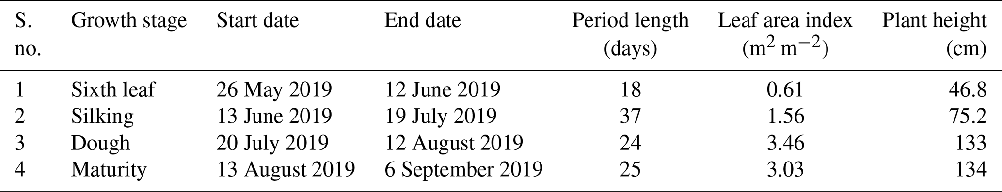
Table 1 shows the phenological stages of the maize crop in the study area (Soujanya et al., 2021). Additionally, leaf area index (LAI) and mean plant height were monitored during the crop cycle (Table 1). The LAI was measured using the plant canopy analyser, whereas the plant height was measured using a ruler from the base of the plant to its crown. Maize crops in the experimental fields were sown on 25 May 2019 and harvested on 6 September 2019, with a base period of 104 d.

Table 1 Phenological growth stages and physical properties of the maize crop.

Data from the EC system at a 10 Hz frequency were converted to ASCII format using LoggerNet (4.3) software (Campbell Scientific Inc., Logan, Utah, USA), and further aggregated to various averaging periods (1, 5, 10, 15, 30, 45, 60, and 120 min). Data post-processing was done using EddyPro post-processing software (version 7.0.8, LI-COR, USA). Primary corrections performed on the raw dataset include tilt corrections, turbulent fluctuations, density fluctuations, frequency corrections, and quality checks. Tilt corrections were done using the double-axis rotation method for each averaging period. Both the block average method and the linear trending method were considered to compute the turbulent fluctuations. The block averaging method was used for detrending the fluxes at the 1, 5, 10, 30, 45, and 60 min averaging periods. Longer averaging periods (e.g. 120 min) resulted in inconsistency in the obtained fluxes, which is a weakness of block averaging (Renhua, 2005; Sun et al., 2006). Hence, the linear trend removal method was used to compute the fluxes for the 120 min averaging period. Density fluctuation corrections were done using the Webb–Pearman–Leuning (WPL) method. Quality checks were performed following a flagging policy proposed by Mauder and Foken, 2006 (0–1–2 system). A flag set to “0” corresponds to the best-quality fluxes, “1” corresponds to fluxes acceptable for general analysis, and “2” corresponds to poor-quality fluxes that should be removed from the dataset. The resulting fluxes may exhibit spikes, discontinuity, randomness, etc. There is a need to perform secondary corrections on the data that include flux spike removal (Vickers and Mahrt, 1997), friction velocity corrections (to filter nighttime observations), gap filling and uncertainty analysis (Finkelstein and Sims, 2001), skewness and kurtosis removal, spectral corrections, and frequency corrections. To correct flux estimates for low- and high-frequency losses due to instrument setup, intrinsic sampling limits of the devices, and various data processing decisions, spectral corrections were performed. Additionally, slow-sensor meteorological data obtained at 1 min intervals were processed for different time averaging periods using the EddyPro post-processing software (version 7.0.8, LI-COR, USA).

2.3 Effect of time averaging on EBR and EC fluxes

Violation of the law of conservation of energy resulting from the EC-observed energy terms is referred to as energy balance closure (EBC). The available energy (R_n−G) is generally higher than the turbulent fluxes (H+LE), resulting in a positive balance (Eshonkulov et al., 2019) where R_n, G, H, and LE correspond to net radiation, soil heat flux, sensible heat, and latent heat, respectively. Apart from instrument and measurement issues, this lack of energy closure is thought to be partly from averaging periods and coordinate systems (Finnigan, 2004; Finnigan et al., 2003; Gerken et al., 2018). The energy closure fraction, commonly referred to as the energy balance ratio (EBR), is used to evaluate the quality of EC data by examining energy fluxes at the surface (Chen and Li, 2012), given by

$$\begin{array}{}\text{(1)}& {\displaystyle }\text{EBR}={\displaystyle \frac{H+LE}{R_{\mathrm{n}}-G}},\text{(2)}& {\displaystyle }H={\mathit{\rho }}_{\mathrm{a}}{C}_p\stackrel{\mathrm{‾}}{w^{\prime }{T}^{\prime }},\text{(3)}& {\displaystyle }LE=L_{\mathrm{v}}\stackrel{\mathrm{‾}}{w^{\prime }\mathit{\rho }{v}^{\prime }},\end{array}$$

where ρ_a is the air density, C_p is the specific heat of air, w^′ is the wind velocity fluctuation, T^′ is the temperature fluctuation, L_v is the latent heat of vaporization, and ${\mathit{\rho }}_v^{\prime }$ is the H₂O gas concentration fluctuation.

EBR helps to determine the averaging period required to calculate H and LE fluxes over a range of landscapes (Chen and Li, 2012). A high EBR (EBR ≥ 0.7) ensures reliability of EC observations for use with flux estimation (Barr et al., 2006; Kidston et al., 2010).

Eddy fluxes are computed as the covariance between the instantaneous deviation in vertical wind speed (w^′) and scalar component of interest (s^′) from their respective means, given by

$$\begin{array}{}\text{(4)}& F\approx \stackrel{\mathrm{‾}}{{\mathit{\rho }}_{\mathrm{a}}{w}^{\prime }{s}^{\prime }},\end{array}$$

where $\stackrel{\mathrm{‾}}{{\mathit{\rho }}_{\mathrm{a}}}$ is the mean air density and the overbar represents the time average of eddy fluxes, which is of interest in the present study. Depending on the scalar component considered (i.e. temperature; water vapour, H₂O); carbon dioxide, CO₂, concentrations), corresponding eddy fluxes (i.e. sensible heat, latent heat, carbon flux) are computed as below.

$$\begin{array}{}\text{(5)}& {\displaystyle }{F}_{{\mathrm{CO}}_{\mathrm{2}}}\approx \stackrel{\mathrm{‾}}{{\mathit{\rho }}_{\mathrm{a}}{w}^{\prime }{{\mathrm{CO}}_{\mathrm{2}}}^{\prime }}\text{(6)}& {\displaystyle }{F}_{{\mathrm{H}}_{\mathrm{2}}\mathrm{O}}\approx \stackrel{\mathrm{‾}}{{\mathit{\rho }}_{\mathrm{a}}{w}^{\prime }{{\mathrm{H}}_{\mathrm{2}}\mathrm{O}}^{\prime }}\end{array}$$

Ecosystem WUE is then estimated as the ratio of daytime carbon (net primary product) to water fluxes (evapotranspiration), observed considering daytime unstable atmospheric conditions (08:00 to 16:00 LT) given by

$$\begin{array}{}\text{(7)}& \text{WUE}={\displaystyle \frac{\text{NPP}}{\text{ET}}}={\displaystyle \frac{F_{{\mathrm{CO}}_{\mathrm{2}}}}{F_{{\mathrm{H}}_{\mathrm{2}}\mathrm{O}}}}.\end{array}$$

Fluxes originating from real-world sites are composed of both high-frequency (turbulence) and low-frequency (advection) fluctuations, with a spectral gap in between. Isolating the local turbulence component for use with flux studies is achieved by choosing an appropriate averaging period, T₁ (typically 30 min), for fast-response measurements operating at high frequency, T₂ (Sievers et al., 2015). The optimal averaging period (T₁) should be long enough to reduce random error (Berger et al., 2001) and short enough to avoid non-stationarity associated with advection (Foken and Wichura, 1996). The flux estimates (Eq. 2) are further decomposed into frequency-dependent contributions known as co-spectra Co_ws(f) between vertical wind velocity (w) and the scalar of interest (s) for frequencies f (Sievers et al., 2015). For an accurate estimation of the flux, it is essential that the EC method is applied under conditions where the flow is stationary and all eddies carrying flux are sampled. Given that the flow remains stationary, an Ogive serves as a check for the essential requirement to sample all scales carrying the flux. The Ogive function is proposed to check if all low-frequency fluxes are included in the turbulent flux measured with the EC method (Foken et al., 2005; Foken and Wichura, 1996). It is used to investigate the energy balance losses caused by low-frequency fluxes. Ogive analysis is performed to investigate the flux contribution from each frequency range and to arrive at the most suitable averaging period to capture most of the turbulent fluxes (Charuchittipan et al., 2014; Desjardins et al., 1989). The Ogive function thus provides the cumulative sum of co-spectral energy starting from the highest frequency, given by

$$\begin{array}{}\text{(8)}& {\text{Og}}_{\mathrm{ws}}\left(f_{\mathrm{0}}\right)={\int }_{f_{\mathrm{0}}}^{\mathrm{\infty }}{\text{Co}}_{\mathrm{ws}}\left(f\right)\mathrm{d}f.\end{array}$$

The point of convergence on the Ogive plot to an asymptote corresponds to optimal averaging period (T₁) for use in the averaging of high-frequency turbulence fluxes. In other words, the point at which the Ogive plot flattens out represents the optimal averaging period. A total of eight averaging periods, i.e. 1, 5, 10, 15, 30, 45, 60, and 120 min, were considered to investigate the role of time averaging on EBR, EC, and WUE fluxes and further to arrive at the optimum averaging period for use with WUE estimation. The biophysical and physiological characteristics, such as plant height, crop water requirement, LAI, etc., change with respect to the crop growth stage (Chintala et al., 2024) and have a significant effect on the EC fluxes. Since these factors vary over growth stages, time averaging of EC fluxes is separated based on crop growth stage.

2.4 Performance evaluation

The ability of various averaging periods to close the energy balance and compute the EC fluxes is evaluated using three goodness-of-fit indicators, namely (a) the coefficient of determination (R²), (b) the root-mean-squared error (RMSE), and (c) the relative error (RE). While R² and RMSE aim to quantify the error in closing the energy balance, RE aims to compute the error in estimating EC fluxes with a conventional 30 min averaging period relative to the optimal averaging period.

The root-mean-square error (RMSE) measures overall accuracy in closing the energy balance for a given averaging period by penalizing large errors heavily, given by

$$\begin{array}{}\text{(9)}& \text{RMSE}={\left[{\displaystyle \frac{{\sum }_{i=\mathrm{1}}^n{\left({\left(R_{\mathrm{n}}-G\right)}_i-{\left(H+LE\right)}_i\right)}^{\mathrm{2}}}{n}}\right]}^{\mathrm{0.5}},\end{array}$$

where n is the number of observations.

The coefficient of determination (R²) and the Pearson correlation coefficient (r) are the measures of the strength of the linear association between turbulent fluxes and available energy, given by

$$\begin{array}{}\text{(10)}& R^{\mathrm{2}}={\left\{{\displaystyle \frac{{\sum }_{i=\mathrm{1}}^n\left[{\left(R_{\mathrm{n}}-G\right)}_i-\stackrel{\mathrm{‾}}{\left(R_{\mathrm{n}}-G\right)}\right]\left[{\left(H+LE\right)}_i-\stackrel{\mathrm{‾}}{\left(H+LE\right)}\right]}{\sqrt{\sum {\left[{\left(R_{\mathrm{n}}-G\right)}_i-\stackrel{\mathrm{‾}}{\left(R_{\mathrm{n}}-G\right)}\right]}^{\mathrm{2}}{\left[{\left(H+LE\right)}_i-\stackrel{\mathrm{‾}}{\left(H+LE\right)}\right]}^{\mathrm{2}}}}}\right\}}^{\mathrm{2}},\end{array}$$

$$\begin{array}{}\text{(11)}& r=\left\{{\displaystyle \frac{{\sum }_{i=\mathrm{1}}^n\left[{\left(R_{\mathrm{n}}-G\right)}_i-\stackrel{\mathrm{‾}}{\left(R_{\mathrm{n}}-G\right)}\right]\left[{\left(H+LE\right)}_i-\stackrel{\mathrm{‾}}{\left(H+LE\right)}\right]}{\sqrt{\sum {\left[{\left(R_{\mathrm{n}}-G\right)}_i-\stackrel{\mathrm{‾}}{\left(R_{\mathrm{n}}-G\right)}\right]}^{\mathrm{2}}{\left[{\left(H+LE\right)}_i-\stackrel{\mathrm{‾}}{\left(H+LE\right)}\right]}^{\mathrm{2}}}}}\right\}.\end{array}$$

The relative error (RE) provides the disparity in the fluxes estimated by conventional (30 min) averaging relative to the fluxes estimated by the optimal averaging period, given by

$$\begin{array}{}\text{(12)}& \text{RE}=\left[{\displaystyle \frac{\left\{F_{\mathrm{opt}}-F_{\mathrm{30}\min }\right\}}{F_{\mathrm{opt}}}}\right]\times \mathrm{100},\end{array}$$

where F_opt and F₃₀ are the fluxes of interest considering optimal and conventional (30 min) averaging periods.

The averaging period corresponding to high R² (close to 1) and low RMSE (close to zero) is considered to be the optimal choice in representing the EC fluxes.

3 Results and discussion

3.1 Diurnal variations in energy balance components

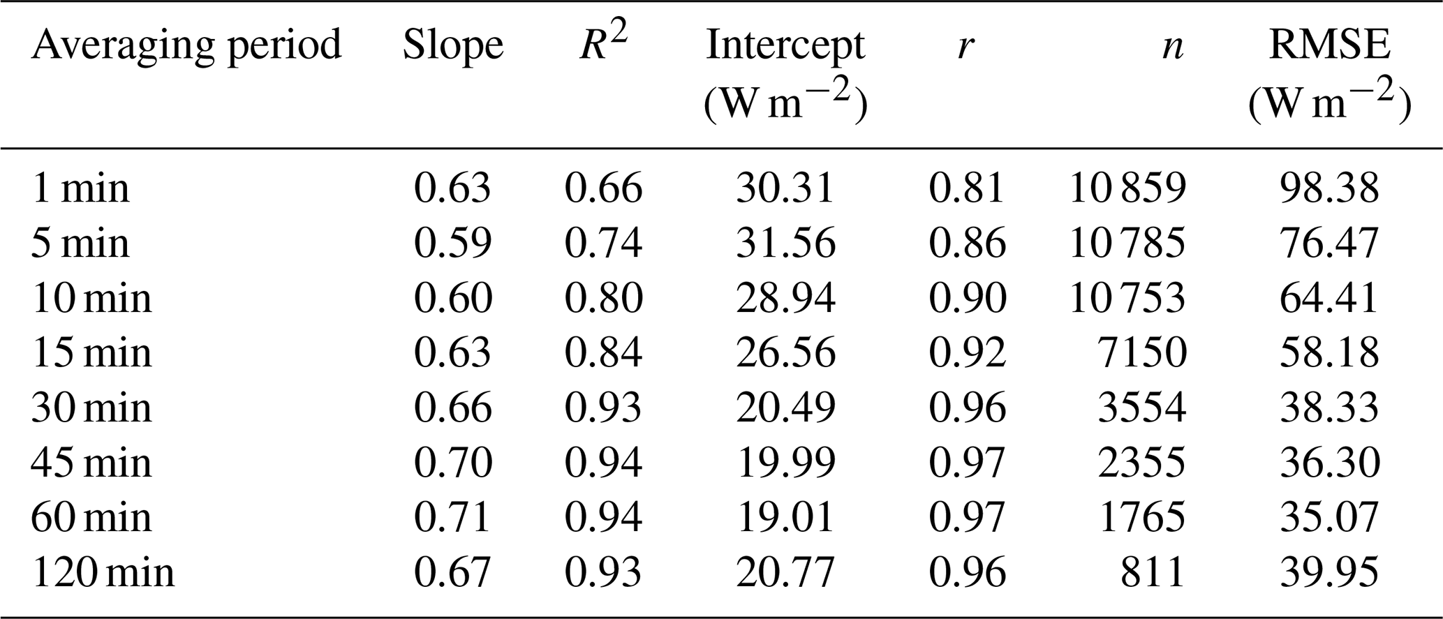
To understand the energy variation in response to rapid changes in meteorological conditions, we analysed the diurnal variations in energy balance components. Figure 1 shows the diurnal variations in available energy (R_n−G) and turbulent fluxes (H+LE) averaged over the crop cycle for various time averages. The diurnal variations in R_n−G and H+LE are bell-shaped, with peaks occurring at around noon (480.16 ± 14.15 W m⁻², 356.23 ± 18.51 W m⁻²; Fig. 1). The energy balance difference (shaded areas of the figure) is found to be positive (76.88 ± 43.14 W m⁻²) during daylight hours (08:00 to 18:00 LT) and is negative (−24 ± 11.65 W m⁻²) for the remaining time. The vertical offset between the two curves, representing the residual of energy balance, is highest around noon (142.39 ± 19.42 W m⁻²) and is consistent between the averaging periods. For an average site-day, the cumulative energy balance difference was found to be constant, with a mean of 1811 W m⁻² at all averaging periods. The cumulative energy balance difference crosses the zero line at around 11:30 LT. The variation is rough at lower averaging periods due to a high sample size (n = 10 859 at T = 1 min) and is gradually smoothed towards higher averaging periods (n = 811 at T = 120 min). The shorter averaging periods have introduced random uncertainty in the datasets during coordinate rotation correction. The slope of regression lines between H+LE and R_n−G considering all averaging periods are in the range of 0.59 to 0.71, with a mean of 0.65. The intercept ranges from 19.01 to 31.56 W m⁻². The best slope (≥ 0.70) and intercept (≤ 20 W m⁻²) were achieved with the 45 and 60 min averaging periods, which is consistent with the literature (Gao et al., 2017; Leuning et al., 2012). We conclude that longer averaging periods have good closure over shorter averaging periods. The strength of the linear association between R_n−G and H+LE around the best fit line explained by r is high (0.80 < r ≤ 0.9) at low averaging periods, i.e. 1, 5, or 10 min, and is very high (r > 0.9) for other averaging periods (Table 2). However, the departure of the data from the 1:1 line is relatively low for both short and long averaging periods. Our findings show that the averaging period has a minimal influence on the representation of the energy balance terms. However, the data scatter around the 1:1 line is high for shorter time averages due to large sample size and data randomness.

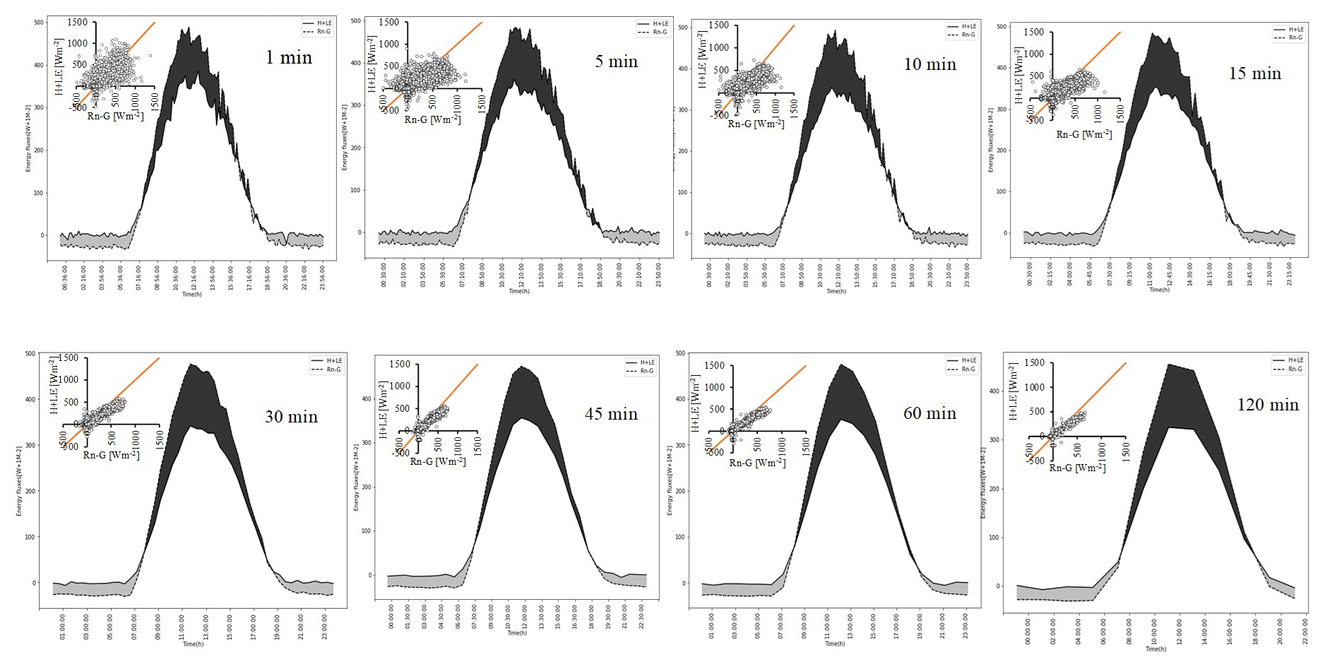
Figure 1 Diurnal variations in energy balance components (available energy is R_n−G and turbulent fluxes are H+LE) during the crop cycle with different averaging periods. Insets show scatterplots between the two datasets.

Table 2 Summary of linear regression parameters in closing the energy balance with different averaging periods.

3.2 Effect of averaging period on EBR and EC fluxes

The variation in energy balance ratio (EBR) by averaging period for individual growth stages of the crop is presented in Fig. 2. We observed a clear departure of EBR from unity for all growth stages, particularly in the dough and maturity stages due to ignorance of canopy heat storage, low-frequency flux losses, and inadequate averaging period (Meyers and Hollinger, 2004; Rahman et al., 2019). EBR fluctuates between 0.70 and 0.90 at low (1–30 min) averaging periods and is fairly constant (mean = 0.75) at high (≥ 30 min) averaging periods. Our reported values of EBR during the crop growth are within the range of 0.65 to 1.2 typically found for most of the crops (Feng et al., 2017; Finnigan et al., 2003; Wilson et al., 2002). The mean EBR with a conventional 30 min averaging period was found to be 0.74, 0.76, 0.71, and 0.74 during the sixth leaf, silking, dough, and maturity stages, respectively. Low EBR during the crop cycle can also be attributed to the ignorance of energy transport associated with large eddies from landscape heterogeneity (Meyers and Hollinger, 2004; Rahman et al., 2019). However, the EC method assumes that the landscape within the footprint of measurement is flat and homogeneous. We did not observe variations in optimal averaging time due to changes in wind speed and direction; hence meteorological conditions were not analysed in this study. Changes in daytime mean carbon and water fluxes by averaging period for different growth stages of the crop are shown in Fig. 3. Carbon fluxes (sink) have a very low mean (1.81 $\mathrm{\mu }\mathrm{mol}{\mathrm{m}}^{-\mathrm{2}}{\mathrm{s}}^{-\mathrm{1}}$) during the sixth leaf stage, a low mean during the silking (3.48 $\mathrm{\mu }\mathrm{mol}{\mathrm{m}}^{-\mathrm{2}}{\mathrm{s}}^{-\mathrm{1}}$) and dough (3.03 $\mathrm{\mu }\mathrm{mol}{\mathrm{m}}^{-\mathrm{2}}{\mathrm{s}}^{-\mathrm{1}}$) stages, and a high mean (15.44 $\mathrm{\mu }\mathrm{mol}{\mathrm{m}}^{-\mathrm{2}}{\mathrm{s}}^{-\mathrm{1}}$) during the maturity stage.

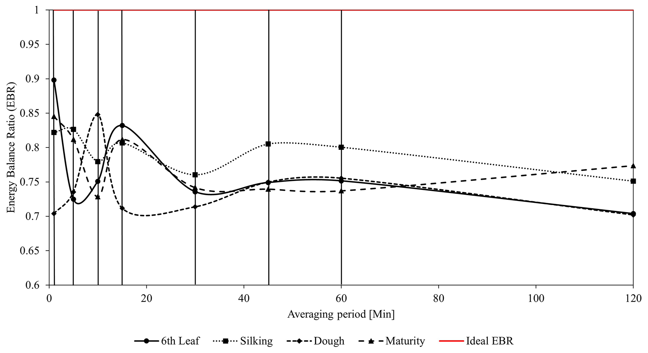
Figure 2 Variations in energy balance ratio (EBR) by averaging period for different growth stages. (solid vertical lines from left to right correspond to the averaging periods of 1, 5, 10, 15, 30, 45, 60, and 120 min, respectively).

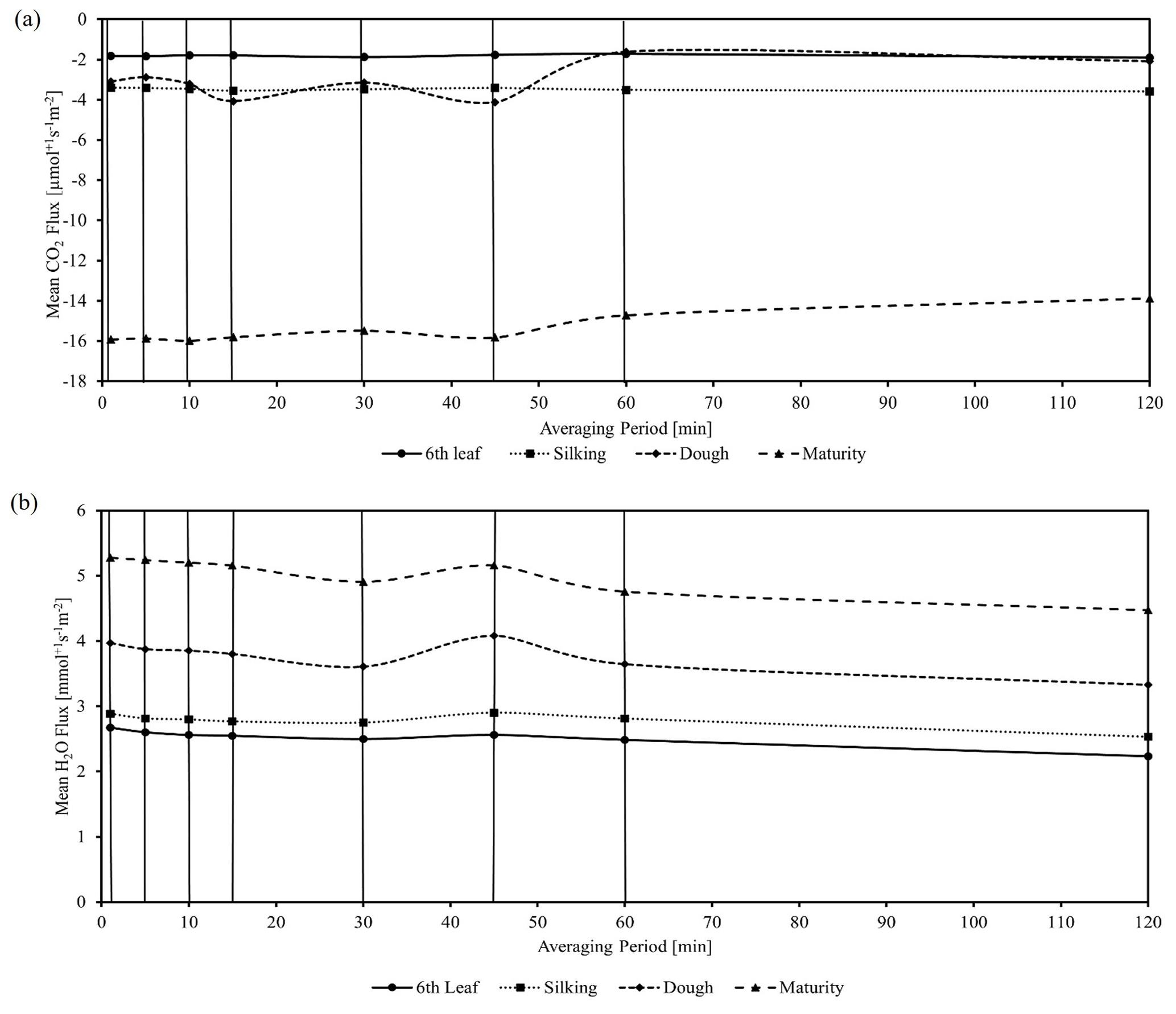
Figure 3 (a) Variations in mean carbon fluxes by averaging period for different growth stages. (b) Variations in mean water fluxes by averaging period for different growth stages (solid vertical lines from left to right correspond to the averaging periods of 1, 5, 10, 15, 30, 45, 60, and 120 min, respectively).

Mean carbon fluxes during the sixth leaf and silking stages are mostly unaffected by the averaging period. We observed a gradual increase in water vapour fluxes during the crop cycle from sixth leaf (2.52 ± 0.13 mmol s⁻¹ m⁻²) to maturity (5.02 ± 0.29 mmol s⁻¹ m⁻²). From the mean CO₂ and H₂O flux dynamics, we observed that the drip-irrigated maize crop is acting as a carbon sink in the entire crop season, especially in the latter stages of the crop, i.e. the maturity stage, with a mean of 15.44 $\mathrm{\mu }\mathrm{mol}{\mathrm{m}}^{-\mathrm{2}}{\mathrm{s}}^{-\mathrm{1}}$. This is clearly evident from the increasing trend of LAI and plant height during the crop season. Such an increase is highlighted by previous studies of Guo et al. (2021). At the same time, mean H₂O fluxes were increased towards the end of the crop growing season due to increased crop water demand. As the averaging period increased, the mean water vapour flux decreased, with an exception at the 45 min averaging period. The deviation in representing carbon and water fluxes at different averaging periods, relative to the conventional 30 min averaging period, i.e. relative error (RE), is presented in Fig. 4. The RE is obtained by considering daily averages in the deviations for each growth stage. During the sixth leaf and silking stages, RE in estimating carbon fluxes is high (∼ −15 %) with low averaging periods and gradually diminishes towards higher averaging periods, with an exception at the very high (120 min) average period. For the dough and maturity stages, RE is found to be significant with higher averaging periods (60–120 min). RE in estimating water vapour fluxes is found to be insignificant at all averaging periods for the sixth leaf and silking stages. However, the dough and maturity stages have shown a large variation in RE considering either too-short (1, 5 min) or too-long (60, 120 min) time averages. A high variation in RE for timescales larger than 45 min indicates the effects of submesoscale (non-turbulent) motions. Hence, the 45 min average period can be considered optimal in isolating the turbulence components for use with flux representation.

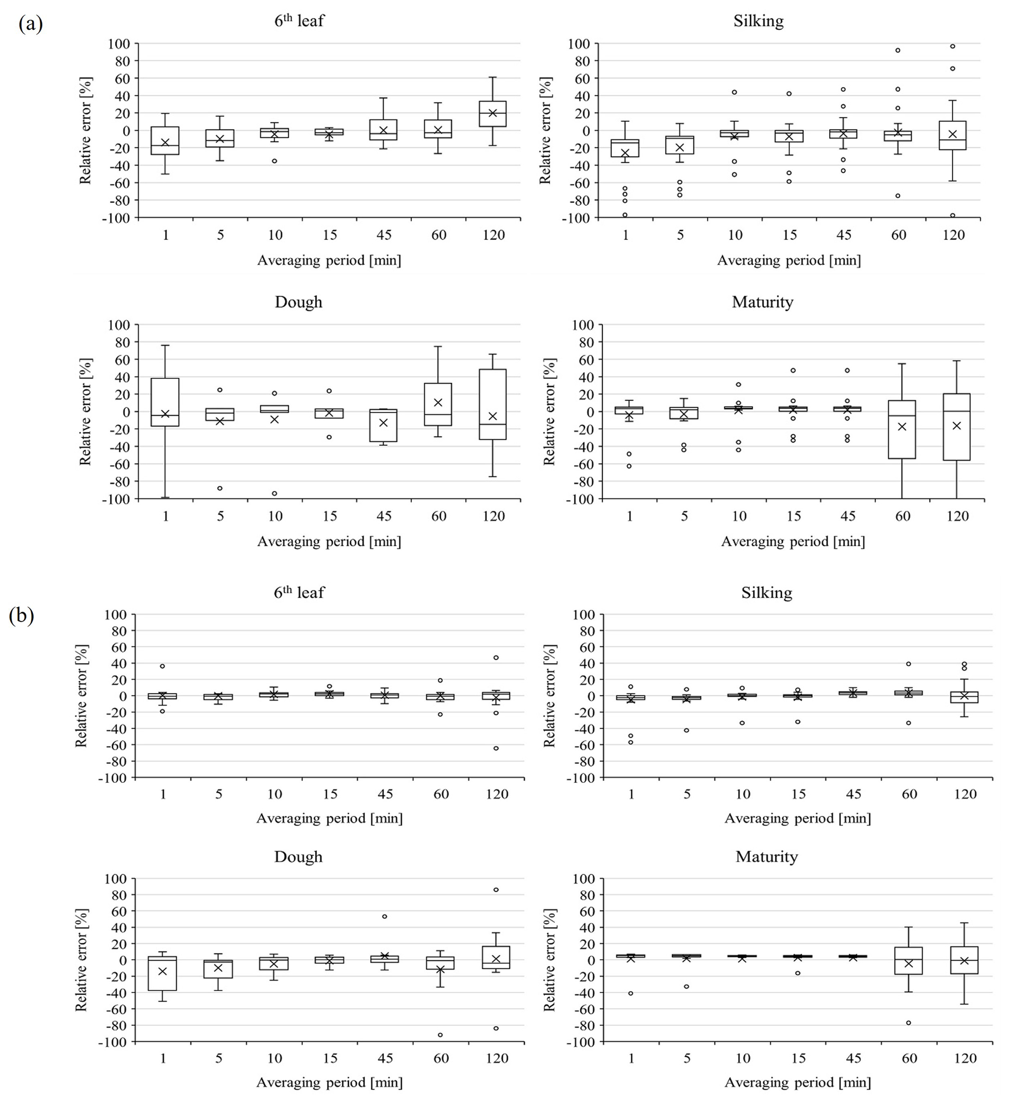
Figure 4 (a) Whisker plots showing the distribution of error in estimating carbon fluxes by various averaging periods relative to the conventional 30 min averaging. (b) Whisker plots showing the distribution of error in estimating water fluxes by various averaging periods relative to the conventional 30 min averaging.

3.3 Selection of optimal averaging period

Ogive functions representing the cumulative integral of the co-spectral energy starting with highest frequency, i.e. 0.016 Hz (T = 1 min), for carbon, water, and WUE fluxes are presented in Fig. 5. Shorter time periods corresponding to daytime unstable atmospheric conditions (08:00 to 16:00 LT) for various growth stages were investigated. Ogive plots of carbon fluxes for the sixth leaf and silking stages showed an increasing trend up to 0.011 Hz (15 min) and remained fairly constant before 0.0055 Hz (30 min). We conclude that whole turbulent spectrum can be covered by 15 to 30 min averaging, with negligible flux contribution from longer frequencies. Ogive plots of carbon fluxes for the dough and maturity stages showed a continuous increasing trend without a defined plateau (horizontal asymptote) in between. This shows that the conventional 30 min averaging period is inadequate to capture the low-frequency fluxes, thus there is demand for higher averaging periods. We observed a similar behaviour with water fluxes (Fig. 5b). The flat part of the Ogive curve representing the optimal averaging period was found to vary across the crop cycle. While a 15–30 min time average is suitable for aggregating the EC fluxes during the sixth leaf and silking stages, 45–60 min averaging is more appropriate for the dough and maturity stages. Similar to carbon and water fluxes, the Ogive plots for WUE are presented in Fig. 5c. From this, we observed that the flat part of Ogive curve is achieved at the 15 min time average period for the stages of sixth leaf and silking and at the 45 min time average for the dough and maturity stages, which is similar to the carbon and water fluxes. This lets us conclude that the WUE co-spectrum followed a similar behaviour to its individual fluxes, i.e. carbon and water fluxes, in achieving optimal time averages. The crop biophysical factors like LAI and plant height are at a minimum during the sixth leaf and silking stages, which contributes a low quantity of CO₂ and H₂O fluxes (see Fig. 3a and b), whereas they are at a maximum in the later stages of the crop, i.e. dough and maturity, contributing to high quantities of CO₂ and H₂O fluxes (see Fig. 3a and b). Our results are in accordance with the previous studies of Fong et al. (2020) on cotton, where the responses in NPP and ET were related seasonally to plant growth stages. The previous studies on various crops revealed that the NPP and ET fluxes were initially low in the early stages and increased towards the maturity stage due to crop phenology and management practices. To capture these low-quantity fluxes, low averaging periods, i.e. 15 min, were sufficient, whereas a 45 min time averaging period can capture high-quantity fluxes that are prevalent during later growth stages of the crop. As the crop characteristics are dependent on crop growth stages, a single time averaging period is not appropriate for capturing the dynamics of CO₂ and H₂O fluxes as well their ratio, WUE. This clearly demonstrates that as the plant achieves its higher stages, the flux contribution from low-frequency components becomes more predominant. Very low averaging periods (i.e. 1 min, 5 min) were found to be unsuitable to capture low-frequency flux components, which is in agreement with the literature (Feng et al., 2017).

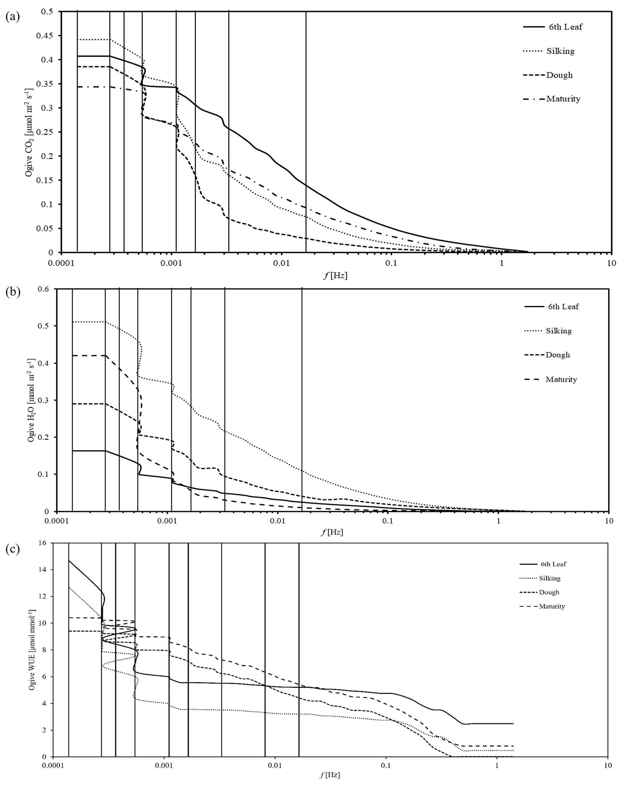
Figure 5 (a) Ogive plots of carbon fluxes for different growth stages of the maize crop. (b) Ogive plots of water fluxes for different growth stages of the maize crop. (c) Ogive plots of water use efficiency for different growth stages of the maize crop. (solid vertical lines from left to right correspond to the averaging periods of 120, 60, 45, 30, 15, 10, 5, and 1 min, respectively.)

3.4 Dynamics of water use efficiency

Daily means of water use efficiency (WUE) estimated with conventional 30 min and growth-specific optimal averaging periods are presented in Fig. 6. Mean WUE fluxes for the sixth leaf, silking, dough, and maturity stages with conventional 30 min averaging are 1.48, 1.36, 1.38 and 3.184 µmol mmol⁻¹ respectively. Corresponding fluxes with stage-specific optimal averaging periods are 1.49, 1.37, 1.39, and 3.06 µmol mmol⁻¹, respectively. The error in estimating mean daily WUE fluxes with 30 min averaging is very low (< 1.45 %) during the sixth leaf and silking stages, low (8.56 % to 9.04 %) during the maturity stage, and moderate (11.84 % to 12.12 %) during the dough stage. We conclude that choice of optimal averaging period is more crucial for late-stage growth periods of the crop. Distribution of error in estimating WUE fluxes with various averaging periods relative to the conventional 30 min average period (RE) is presented in Fig. 7. A close-to-zero RE with all averaging periods during the sixth leaf and silking stages shows that the choice of averaging period has an insignificant role in estimating the WUE fluxes, particularly during early growth stages. A slightly high RE (∼ −5.4 %) during the dough and maturity stages shows that the choice of averaging period matters for WUE estimation during late-stage periods. Hence, the conventional 30 min averaging period can be considered for estimating WUE fluxes during the sixth leaf and silking stages, whereas the optimal averaging period needs to be considered for estimating WUE fluxes during the dough and maturity stages. Correlation charts showing the linear association considering daily means of carbon, water, and WUE fluxes at different averaging periods are represented in Fig. 8. For ease of comparison, data for the entire crop cycle were considered. Linear association between any two averaging periods is positive (r > 0.56) for carbon and water fluxes. Except for the 120 min time averaging, all other averaging periods are strongly correlated (r > 0.87) with the 30 min averaging period. Surprisingly, poor linear association in WUE fluxes was observed between any two averaging periods, which is attributed to a larger variation in individual WUE fluxes between averaging periods. However, the corresponding individual carbon and water fluxes have recorded low variations between time averages. We conclude that the need for an optimal averaging period is crucial in representing WUE fluxes rather than individual carbon and water fluxes. Our findings can improve representation of WUE fluxes using EC data, thereby helping to develop efficient water management strategies in response to WUE changes.

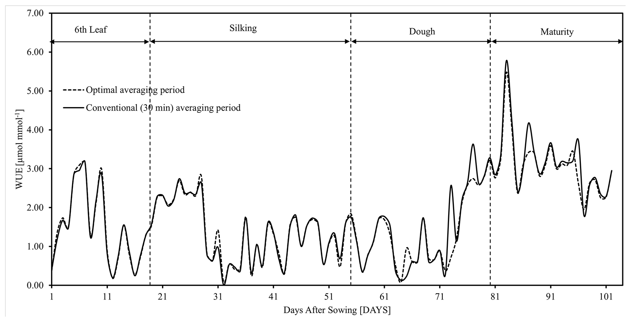
Figure 6 Seasonal variations in daily mean WUE fluxes obtained using conventional 30 min averaging periods (solid lines) and optimal averaging periods (dotted lines) during the crop cycle.

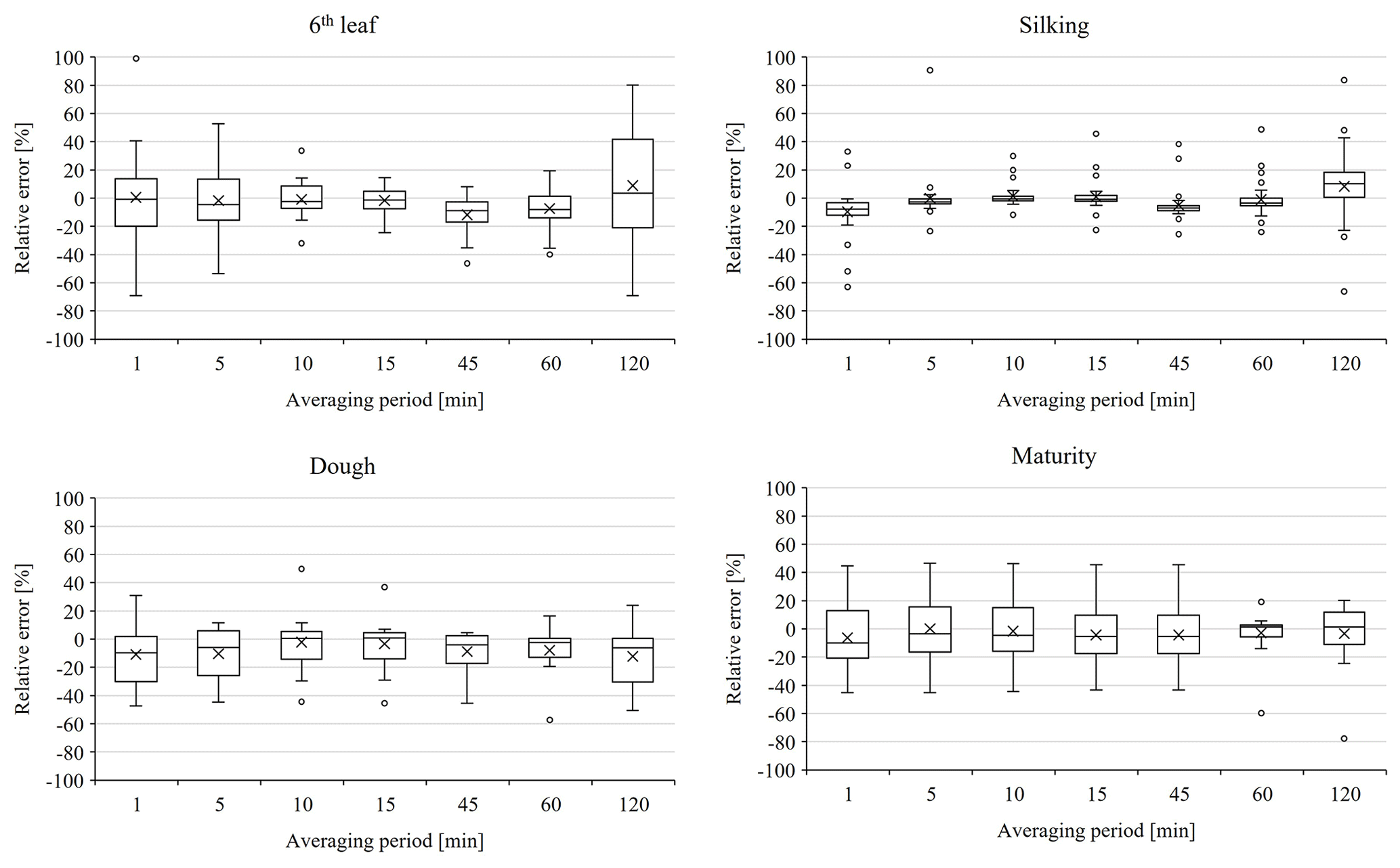
Figure 7 Whisker plots showing the distribution of error in estimating WUE fluxes by various averaging periods relative to the conventional 30 min averaging.

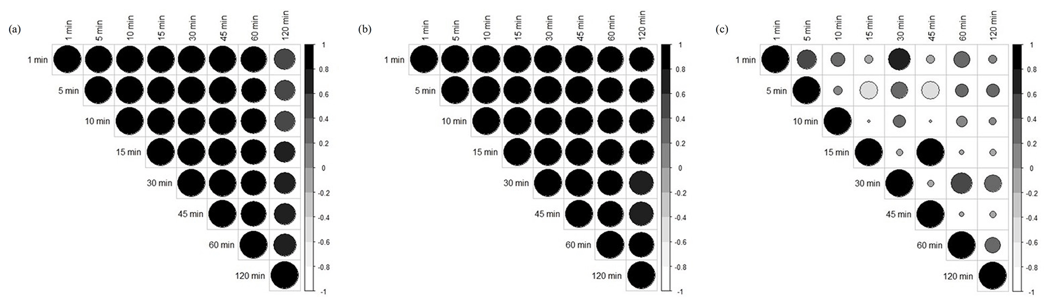
Figure 8 Correlation charts showing the linear association of (a) carbon fluxes, (b) water fluxes, and (c) WUE fluxes estimated by different averaging periods. The circle size represents the correlation magnitude and the colour intensity from white to black represents the negative to positive correlations, respectively.

4 Conclusions

This study explores the effect of the averaging period of EC fluxes on EBR dynamics and WUE in semi-arid Indian conditions. The proposed methodology was applied to a drip-irrigated maize field for one crop period (May–September 2019). Major findings of this study are as follows.

• EBR was found to vary marginally at low averaging periods and less significantly during higher averaging periods.

• With reference to the conventional 30 min averaging period, the relative error is within 12 % for the 10–45 min averaging periods for carbon fluxes and is within 5 % for the 15–45 averaging periods for water fluxes.

• From Ogive analysis, we found an optimal averaging period of 15–30 min for the sixth leaf and silking stages and of 45–60 min for the dough and maturity stages.

• The mean carbon fluxes increased from 1.81 $\mathrm{\mu }\mathrm{mol}{\mathrm{m}}^{-\mathrm{2}}{\mathrm{s}}^{-\mathrm{1}}$ (sixth leaf stage) to 15.44 $\mathrm{\mu }\mathrm{mol}{\mathrm{m}}^{-\mathrm{2}}{\mathrm{s}}^{-\mathrm{1}}$ (maturity stage), which indicates that the carbon sink is a function of the crop growth period. In case of water fluxes, they increased from 2.52 mmol m⁻² s⁻¹ (sixth leaf stage) to 5.02 mmol m⁻² s⁻¹ (maturity stage). Variations in carbon and water fluxes directly influence WUE dynamics.

• The variation in WUE increased subsequently with the plant growth and achieved its maximum value of 5.17 µmol mmol⁻¹ in between the dough and maturity stages, which shows that the crop consumed more carbon than water as the crop period progressed.

• The correlation between CO₂ and H₂O fluxes for all averaging periods was found to be high. However, WUE, which is calculated as the ratio of CO₂ and H₂O fluxes, did not follow the same pattern. While 45 and 15 min averaged WUE exhibits a good correlation, 30 min averaged WUE is not correlated with the other averaging periods. The averaging period is found to be an influencing factor in controlling WUE, hence it should be considered with caution during the crop growth.

This study is limited to understanding the role of different time averaging periods on EC-observed carbon and water fluxes, as well as EC-derived WUE fluxes contributed by the homogeneous maize crop, which has a relatively small flux footprint in unstable atmospheric conditions. The study findings can help to accurately characterize the WUE of the maize crop, considering growth stages for effective implementation of irrigation strategies.