Pre-launch calibration and validation of the Airborne Hyper-Angular Rainbow Polarimeter (AirHARP) instrument

The Airborne Hyper-Angular Rainbow Polarimeter (AirHARP) is a new imaging polarimeter instrument capable of sampling a single Earth target from up to 120 viewing angles, in four spectral channels, and in three linear polarization states across a 114° field of view (FOV). AirHARP is telecentric in the image space and simultaneously images three linear polarization states with no moving parts. These two aspects of the design allow for a simple and efficient quantitative calibration. Using coefficients derived at the center of the lens and the detector flatfields, we can calibrate the entire AirHARP sensor in a variety of laboratory, field, and space environments. We show that this telecentric calibration technique yields a 1σ absolute uncertainty of 0.25 % in degree of linear polarization (DOLP) in the laboratory for all channels and for pixels around the optical axis. To validate across the FOV, we compare our multi-angle reflectance and polarization data with the Research Scanning Polarimeter (RSP) over targets sampled during the NASA Aerosol Characterization from Polarimeter and Lidar (ACEPOL) campaign. We use the error-normalized difference technique to estimate how well the instruments compare relative to their error models. We find that AirHARP and the RSP reasonably agree for reflectance and DOLP within 2 standard deviations of their mutual uncertainty at 550, 670, and 870 nm and over a limited set of ocean and desert scenes. This calibration technique makes the Hyper-Angular Rainbow Polarimeter (HARP) design attractive for new spaceborne climate missions: HARP CubeSat (2020–2022), HARP2 (2024–) on the NASA Plankton, Aerosol, Cloud, ocean Ecosystem (PACE), and beyond.

1 Introduction

Aerosols and their effect on clouds are one of our largest climate challenges. These particles are difficult to model and measure from satellites. Some aerosols are irregularly shaped, absorbing, and dimly reflecting, and others are spherical and efficient at scattering sunlight. They are transported across the globe from a variety of source regions, perturb the boundary layer, and interact with clouds in different ways, depending on their location in the atmosphere and composition. Aerosols can control how long clouds last, how bright they are, and when they will precipitate (Boucher et al., 2013). This complexity makes it difficult to estimate the impacts of clouds and aerosols on our climate system. However, this uncertainty drives innovation and instrument development. Satellite measurements with a range of spectral, angular, spatial, and polarized capabilities can improve how we measure these properties at global scales (NASA, 2018). Instruments that combine these features, called multi-angle polarimeters (MAPs), may make considerable enhancements to our climate record in this direction (Dubovik et al., 2019). They are highly compatible with current instruments, expand the information content possible in a single measurement, and can be designed to small and cost-effective form factors. Recent studies show that microphysical retrievals done on MAP data are highly attractive for future missions and improving our knowledge of microphysical properties (Mishchenko et al., 2004; Knobelspiesse et al., 2012; Stamnes et al., 2018; Remer et al., 2019). Of these, those that sample with less than or equal to 3 % uncertainty in absolute radiometric calibration and 0.5 % absolute uncertainty in the degree of linear polarization (DOLP) are optimal (NASA 2015, 2021).

Over the past decade, several research teams have demonstrated a variety of effective MAP designs in aircraft campaigns and laboratory calibrations. Prominent MAP instruments include the Research Scanning Polarimeter (RSP; Cairns et al., 1999), the SPEX (Hasekamp et al., 2019), the Airborne Multi-angle Spectro-Polarimetric Imager (AirMSPI; Diner et al., 2013), the MAP as part of the spectrometer of the Munich Aerosol and Cloud Scanner (specMACS) instrument (Weber et al., 2024), and the Hyper-Angular Rainbow Polarimeter (HARP; Martins et al., 2018). The RSP is a 14 mrad single-pixel scanner that measures polarized radiation from a target pixel at up to 150+ viewing angles. The RSP measures these angles across nine spectral channels from 410 to 2200 nm. Its narrow viewing angle density (0.8°), together with a high polarimetric uncertainty (∼ 0.002 in DOLP), allows for a near-seamless reconstruction of the scattering profile of any ground target. RSP measurements paved the way for new cloud and ice property retrievals (Sinclair et al., 2021; van Diedehoven et al., 2013), ocean color (Chowdhary et al., 2012), and improved cross-comparisons with other instruments (Knobelspiesse et al., 2019; van Harten et al., 2018; Smit et al., 2019). The RSP represents one possible MAP design, but there are others that take advantage of spectral information and modulation of the polarized signal. The SPEX instrument is a hyperspectral multi-angle polarimeter capable of measuring a ground target from five to nine viewing angles over 109 spectral channels (400–800 nm). SPEX selects wavelengths using an internal diffraction grating and uses spectral modulation to deconvolve total radiance and DOLP signals from the measurements. SPEX measurements may narrow uncertainty in aerosol microphysical retrievals of single-scattering albedo, size, shape, and refractive indices, beyond the capabilities of current space platforms (Hasekamp and Landgraf, 2007; Hasekamp et al., 2019). Also, the highly accurate (∼ 0.002 in DOLP) SPEX was one of the polarimeters that contributed to the NASA Plankton, Aerosol, Cloud, ocean Ecosystem (PACE) mission, specifically for new aerosol science (Werdell et al., 2019; Rietjens et al., 2019). The AirMSPI instrument measures the incident polarization state of a target using photo-elastic modulation (Diner et al., 2013). AirMSPI tracks the same point on the ground with a programmable gimble that locks into specific view angles (step and stare). In a separate sampling mode, the MSPI scans a pushbroom focal plane array (FPA) over a wide range of scattering angles (continuous sweep). The MSPI concept was optimized into the Multi-Angle Imager for Aerosols (MAIA), a space mission that will characterize air pollution over city targets (Diner et al., 2018). The AirMSPI team reports < 0.005 DOLP uncertainty for all spectral channels, which is achieved and further improved by aggregating pixels (van Harten and Diner, 2015; van Harten et al., 2018; Knobelspiesse et al., 2019). Finally, the MAP on specMACS is a dual-camera, wide-FOV (field-of-view) sensor with a division-of-focal-plane polarimetric design and a three-band visible Bayer filter on each detector. Both cameras are positioned symmetrically off-nadir, such that both FOVs overlap for some pixels and contain unique spatial coverage in others. The angular density is the sharpest of any MAP (0.3°), which was recently demonstrated in high-resolution cloud retrieval studies (Pörtge et al., 2023).

This paper discusses the HARP, a wide-field, Earth-observing modern MAP that is capable of highly resolved, highly accurate climate measurements. This work focuses on AirHARP, the aircraft version of the HARP design. The work will discuss the optics of the instrument, how it combines the strengths of the above instruments, and how our calibration process maintains high measurement accuracy in the laboratory and in the field. In this paper, we introduce the AirHARP instrument (Sect. 2), step through the full quantitative calibration process in detail (Sect. 3), and discuss validation studies done in the laboratory and on flight data (Sect. 4). We close in Sect. 5 with a discussion of limitations and look ahead to the HARP CubeSat satellite payload and the HARP2 deployment on board the NASA PACE mission in 2023.

2 AirHARP

The AirHARP instrument is a wide-FOV imaging polarimeter shown in Fig. 1. AirHARP samples Earth targets in four nominal channels (bandpasses): 440 nm (16 nm), 550 nm (13 nm), 670 nm (18 nm), and 870 nm (39 nm). These four channels are selected passively using a custom stripe filter on top of a charge-coupled device (CCD) detector FPA. The stripe filter distributes the four AirHARP channels across 120 distinct regions of the detector, called view sectors. The 670 nm band covers 60 of these view sectors, and the other 60 are split equally across the other three bands. AirHARP contains three CCD detectors that each image a component of the incident beam through the optical path. Each detector is covered by a linear polarizer set at a unique angle. This design decouples the incident polarization into orthogonal S and P states at each FPA. In postprocessing, co-located information in each detector is combined to reproduce the Stokes parameters (I, Q, U) of the original beam. Simultaneous polarization imaging by the three detectors, across four spectral channels, allows high polarization accuracy with no moving parts.

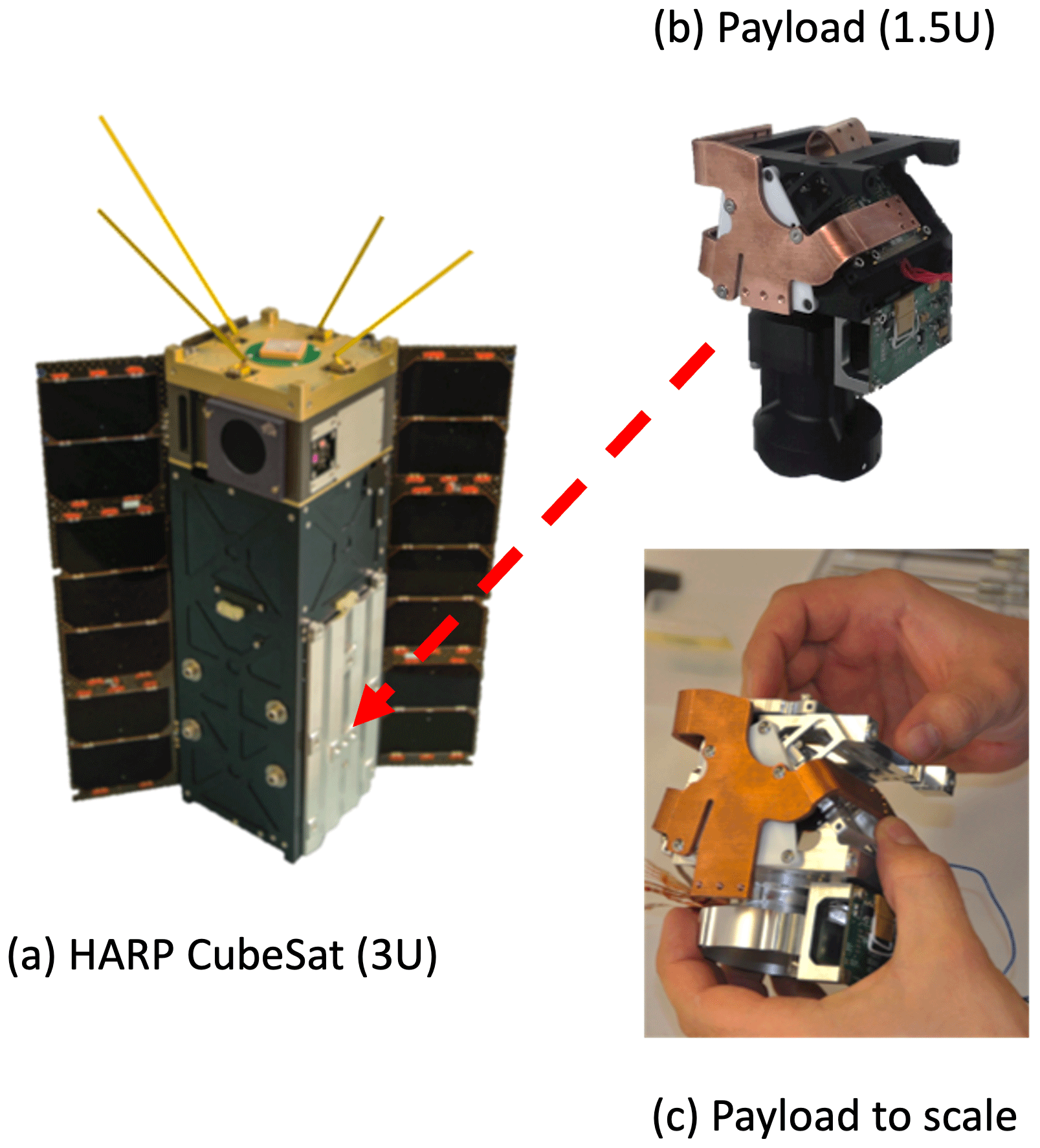
Figure 1 AirHARP is an aircraft demonstration of HARP CubeSat (a), a standalone 3U spacecraft, which carries the same 1.5U instrument (b) in the lower half of the housing. The payload can fit in the palm of a human hand (c).

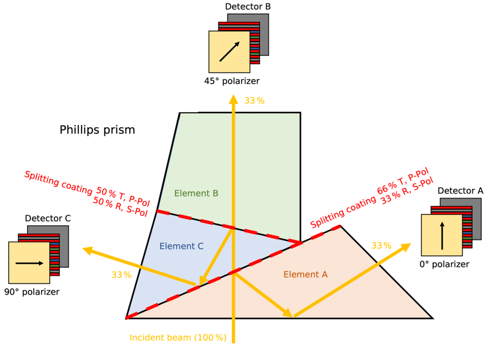
Figure 2 The Phillips prism is made up of three elements: A, B, and C. Two splitting coatings split polarization states by transmission (T) and reflection (R). The coatings ensure that each HARP detector sees ∼ 33 % of the incident beam. The angle of the detector polarizer boosts the polarization efficiency of the prism along that light path. The light encounters the polarizer, stripe filter, and detector FPA.

The core of AirHARP's polarization sensitivity is the custom Phillips prism shown in Fig. 2. While this prism is typically designed to split colors, the AirHARP prism splits the polarization content of the original signal into the three AirHARP detectors. The prism is made of three individual glass elements, A, B, and C, of an equal index of refraction. The prism is a major component of an optical train that contains eight other sequential elements and a 114° wide-field front lens. These lenses are optimized for optical throughput into the prism and create an imaging sensor that is telecentric in the image space. This feature is critical to our calibration and will be discussed in later sections. Most importantly, this refractive design allows wide-FOV measurements in a 3U CubeSat housing (10 × 10 × 30 cm).

The modified Phillips prism alters each detector's light path in a specific way. The incident beam first enters the prism at the front face of Element A and meets the boundary between Elements A and C. A custom splitting coating at the boundary reflects 33 % of this light back into Element A. Reflections like this reduce P-polarization and preserve S-polarization. Transmissions do the reverse. To boost the efficiency of the final polarization measurements, we align the Detector A polarizer with this S-polarization state, which is defined as 0°. The light path defined by the wide-FOV front lens, optical train, prism, 0° polarizer, and Detector A FPA is called Sensor A. The convention of our polarimetric calibration is relative to this sensor. The two other light paths through the optics define Sensors B and C.

The light that passes through this boundary contains primarily P-polarized light. At the interface between Elements B and C, another thin-film coating splits the light intensity into 50 % in reflection and 50 % in transmission. So far, the polarization content of this beam has changed by a transmission through the Element A–C interface and a reflection at the Element B–C interface. Therefore, the light incident on Detector C is a weak mixture of S and P states. The detector polarizer can be set at any angle with minimal effect on polarization efficiency. During optimization testing, we found the best orientation to be 90° for the Detector C polarizer and likewise 45° for the Detector B polarizer. This 45° relative separation between the polarizers is optimal for discriminating between measured states of polarization in our design (Tyo et al., 2006). Sensors B and C each account for 33 % of the intensity of the incident beam as well. Therefore, the AirHARP optics split the incident light intensity equally among the three sensors, each sensor images a spatially identical scene, and each sensor is sensitive to a different angle of polarized light.

Light that passes through the prism and detector polarizer is categorized by a custom interferometric filter on the detector surface. Each detector pixel maps to a specific spectral band, defined by 1 of the 120 view sectors. AirHARP produces a pushbroom of a ground scene in a single view sector by flying over the scene and acquiring images one after the other. The co-located information from multiple view sectors can provide high angular coverage on the cloudbow at 670 nm (McBride et al., 2020) and multi-angle sampling of aerosol optical, shape, size, and loading properties (Hasekamp and Landgraf, 2007; Wu et al., 2015; Puthukuddy et al., 2020) and atmospheric correction (Frouin et al., 2019). Aerosol and cloud properties retrieved by AirHARP (and future HARP instrument) measurements may complement our existing climate record and advance our understanding of climate change uncertainties, feedbacks, and forcings (Boucher et al., 2013).

The AirHARP instrument and spaceborne version, the HARP CubeSat, was funded by the NASA Engineering Science and Technology Office InVEST program as a demonstration of advanced, miniaturized Earth science technology for future satellite missions. The HARP CubeSat recently completed a 2-year mission in the 425 km apogee orbit of the International Space Station. AirHARP was built specifically for science aircraft, like NASA B-200 and ER-2, and demonstrated the HARP design and capabilities in field campaigns before and during the CubeSat mission. AirHARP flew successfully in two NASA aircraft studies in 2017: the Lake Michigan Ozone Study (LMOS) in the summer (McBride et al., 2020) and Aerosol Characterization from Polarimeter and Lidar (ACEPOL) in the fall (Knobelspiesse et al., 2020). A third, highly advanced version of the HARP concept, HARP2, was recently launched on board the NASA PACE mission (McBride et al., 2019). HARP2 achieves global coverage in 2 d and, as of this writing, has taken over 6 months of global radiance and polarization imagery. HARP2 anticipates a nominal mission lifetime of 3 years.

While the calibration discussed in the later sections is the general scheme for any of the HARP instruments, the plots, tables, and figures correspond to the AirHARP instrument unless otherwise noted. Whenever the term “HARP” is used without an “Air” prefix or a “CubeSat” suffix, it is in reference to a general HARP design.

3 Calibration scheme for HARP instruments

3.1 Detector specifications and background correction

The calibration process of AirHARP begins at the detector level. The AirHARP detectors are monochrome CCDs with a 4 MP active FPA (Semiconductor Components Industries, 2015). Relevant properties, such as quantum efficiency, read noise, and dark current, are given in Table 1. The typical images taken by the AirHARP detectors are shown in Fig. 3a. The detector stripe filter creates the cross-track striping in the images seen below. The far-left and right detector pixels are masked, which defines the active science area of the FPA. The pixel values in these areas are compatible with a dark image, which is a snapshot taken when the entire FOV is blocked from illumination (shown in Fig. 3b).

Table 1 Specifications of the AirHARP detectors.

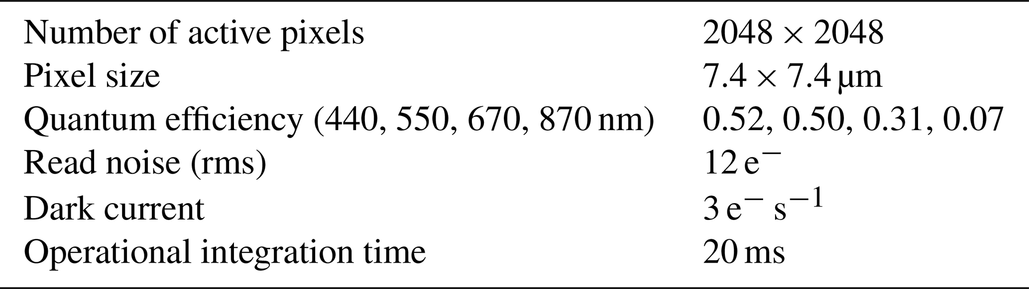
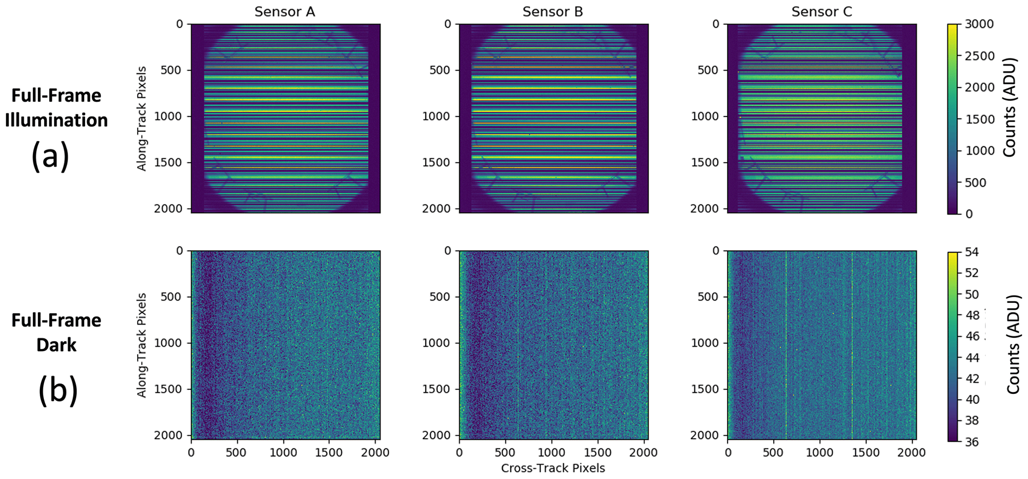
Figure 3 AirHARP captures a full-field raw image in each detector of the aperture of the NASA GSFC “Grande” integrating sphere (a) and a dark capture with the lens cap on (b). The dark capture shown here can be normalized and used as a template for any live data capture.

The first step in the AirHARP calibration begins at the detector level. Detectors generate a stable electrical bias across the FPA when they operate, which must be removed before science analysis. To account for this, we block all illumination from reaching the front lens (i.e., with a lens cap or internal shutter) and take 10 or more sequential images in each detector. These images are averaged together into a dark template. Creating this template image is called the standard process in this work going forward. The typical distribution of the dark template is given in Fig. 3b. The region of lower pixels on the left-hand side of the image is typical of CCDs and can occur as photoelectrons move toward the serial register. A typical dark signal for the AirHARP detectors is 40 counts when operating at room temperature. In general, the background correction is as follows:

$$\begin{array}{}\text{(1)}& {\mathrm{DN}}_{\mathrm{BC}}={\mathrm{DN}}_{\mathrm{raw}}-{\mathrm{DN}}_{\mathrm{dark}},\end{array}$$

where DN_BC is the background-corrected image digital numbers or counts, DN_raw is the raw image counts, and DN_dark represents the dark template counts. Whenever the term raw is used, it refers to any HARP image, whereas subscripts other than raw describe an image captured in a different environment. Furthermore, counts may be called analog–digital units (ADUs) in this work, if relevant.

All HARP iterations have an internal shutter, which is actuated for in-flight dark captures. This shutter does not contribute to polarization imaging and defaults to an open configuration outside the optical path as a fail-safe. If we cannot take dark captures on-orbit or during field campaigns for any reason, we can create a synthetic dark by scaling a normalized dark template from the laboratory with an average of all along-track counts in the vignetted areas of a live data capture (typically over cross-track pixel indices 0–100, seen in Fig. 3b):

$$\begin{array}{}\text{(2)}& {\mathrm{DN}}_{\mathrm{dark}}={\widehat{\mathrm{DN}}}_{\mathrm{dark}}{\stackrel{\mathrm{‾}}{\mathrm{DN}}}_{\mathrm{raw}}^{\ast },\end{array}$$

where DN_dark is the estimated dark image counts and ${\widehat{\mathrm{DN}}}_{\mathrm{dark}}$ is a normalized dark template image from the laboratory. ${\stackrel{\mathrm{‾}}{\mathrm{DN}}}_{\mathrm{raw}}^{\ast }$ represents a spatial mean of pixels in the vignetted area of a raw image capture (similar to Fig. 3a). Equation (2) creates a full-field dark image for each sensor that is used in the following calibration steps and in the L1B processing of AirHARP flight imagery. If Eq. (2) is required, the DN_dark here is substituted into Eq. (1). This technique is currently used to correct AirHARP L1B datasets in Version 002 and accounts for the possibility of internal shutter failure on-orbit.

In the following sections, we limit our discussion to the 670 nm channel, unless otherwise noted. Similar performance for the other three channels can be found in official ancillary basis documents (ACEPOL Science Team, 2017).

3.2 Nonlinear correction

AirHARP sensors are commercial CCDs. They are subject to nonlinearity in their analog-to-digital conversion (ADC). For very bright targets, like sunglint, Earth's limb, or direct solar exposure, pixels may saturate at the top of the detector well (44 000 electrons or 2¹⁴ counts). Saturated pixels cannot convert any extra photoelectrons to counts, but CCDs are known to have a nonlinear gain near saturation and potentially at very low light levels.

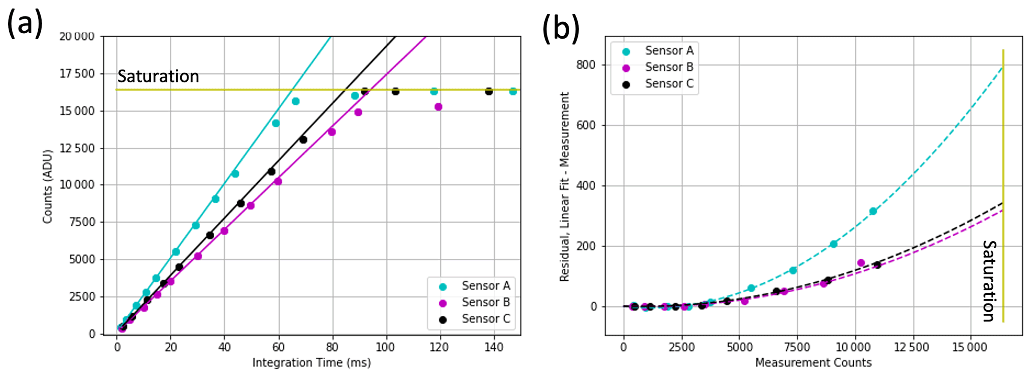
Figure 4 AirHARP detector integration time is varied while imaging a stable light source (670 nm channel shown). The counts in the linear regime (< 3000 ADU) are fit in panel (a) for all the sensors. This linear fit is compared to the entire dataset, and the residual is fit to a three-parameter quadratic (b), which can now correct any raw measurement > 3000 ADU.

The detectors must be well-characterized for accurate science retrievals too. We characterize nonlinearity by taking images of a stable source at a single illumination level. Each image is taken at a longer integration time than the last, and the testing ends when all sensors and channels are saturated. To perform this test, the AirHARP instrument was placed ∼ 1 m from the entrance aperture of the 101.6 cm NASA GSFC “Grande” integrating sphere. The AirHARP detector integration times are set near 4 ms to start. The integration times of each sensor are increased, and images are taken until all three sensors and channels saturate. The stability of the source is tracked over the testing window using a current monitor. The standard process is used to form a template image at each integration time and for each detector. We take a small pixel bin (∼ 4 × 4) along the optical axis in the templates and plot those values against their integration times. This process is performed for each channel and sensor. An example of the 670 nm channel is shown in Fig. 4a for the three AirHARP detectors (Sensor A in cyan, Sensor B in magenta, Sensor C in black). There is a monotonic, positive relationship between integration time and detector counts up until the saturation point, 2¹⁴ ADU. We identify a set of data points with minimal deviation from a linear response (< 3000 ADU) and compare the linear fit over those points to the rest of the data:

$$\begin{array}{}\text{(3)}& {\mathrm{DN}}_{\mathrm{corr}}={\mathrm{DN}}_{\mathrm{linfit}}-{\mathrm{DN}}_{\mathrm{BC}}=n_{\mathrm{0}}{\mathrm{DN}}_{\mathrm{BC}}^{\mathrm{2}}+n_{\mathrm{1}}{\mathrm{DN}}_{\mathrm{BC}}+n_{\mathrm{2}},\end{array}$$

where DN_corr is the nonlinear corrected counts; DN_linfit is the fit performed on the linear region; DN_BC is the count data derived from Eq. (1); and fit parameters n₀, n₁, and n₂ are free parameters. In our Fig. 4b example, the residual (DN_linfit−DN_BC) is the y axis, and the x axis is DN_BC. The maximum nonlinear deviation at 670 nm is ∼ 5 % in Sensor A, found by taking the ratio ${\mathrm{DN}}_{\mathrm{linfit}}/{\mathrm{DN}}_{\mathrm{BC}}$. This ratio agrees with the 6 % nonlinearity limit in the KAI-04070 detector spec, and similar agreement is found for other channels and sensors. Background correction and nonlinearity occur before any other step in the L1B processing pipeline for HARP data. We perform nonlinearity early in the calibration pipeline to check detector-level anomalies. Because the radiometric information in the scene data comes from all three detectors, it is not feasible to characterize linearity during radiometric calibration, like MODIS (Aldoretta et al., 2020). Nonlinear correction early in the calibration pipeline allows for a verification of the reciprocal test during absolute radiometric calibration (counts measured at a single integration time across a variety of lamp levels).

3.3 Flatfielding

Next, we characterize the pixel-to-pixel relative response of each detector. Any system with sequential optical elements will vignette photons toward the edge of the FPA. Individual pixels may have a relative differential gain as well. Both effects must be corrected. To account for this, images are taken of a homogenous target in a process called flatfielding. Integrating spheres are typical sources. They create uniform illumination over their aperture and can depolarize the output to a level below 0.5 % at visible wavelengths (McClain et al., 1994). Therefore, any heterogeneity in the images is due to the instrument, not the source. We use the Grande sphere at NASA GSFC for baseline flatfielding and a portable LED hemisphere at UMBC during field campaigns or between GSFC calibrations. To form the flatfield template, the full FOV of the AirHARP instrument images the aperture of an illuminated integrating sphere, at an integration time where all channels are below saturation. The images are full-size and full-resolution and resemble Fig. 5a. A template image, created using the standard process, is corrected for background and nonlinearity. This template is then interpolated by a smoothing algorithm, row by row. This step captures the structure of vignetting and other potential artifacts, such as optical etaloning and defects on the detector surface.

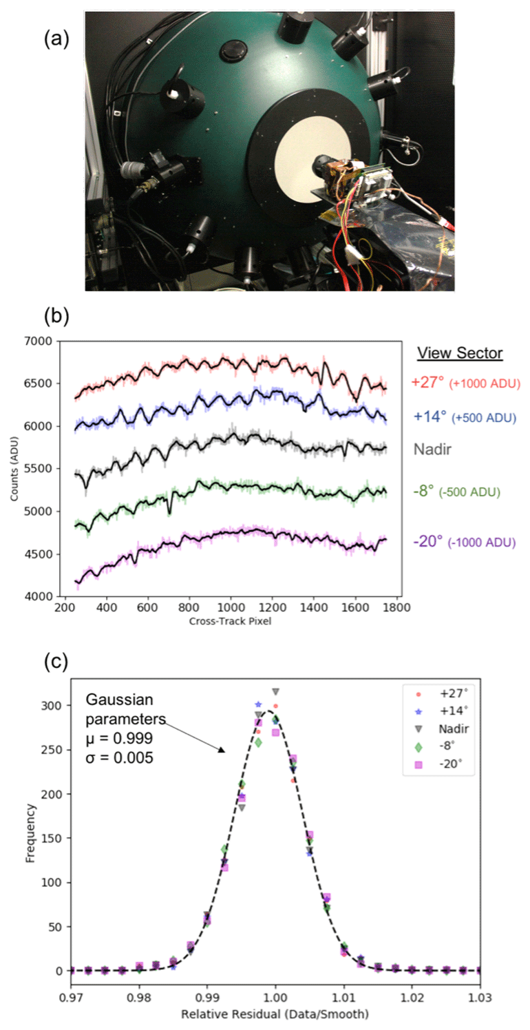
Figure 5 The flatfield is performed by submerging the wide-field front lens in the aperture of an integrating sphere (a). This creates a full-field image similar to Fig. 3a. In panel (b), the cross-track signal for several detector rows (colored data) is smoothed (black curves). After Eq. (3) is applied, only the pixel-to-pixel variations due to noise remain, which are normally distributed within 0.5 % across the FOV. Data in panels (b) and (c) are shown for AirHARP 670 nm.

Figure 5b shows a cross-track line cut for several 670 nm view sectors: +27° (red), +14° (blue), nadir (gray), −8° (green), and −20° (magenta) are shown. The x axis shows the cross-track pixel index. The edge-vignetted detector regions are neglected in the flatfielding process. The y axis shows detector counts (ADU). Each curve is artificially offset by ±500 or 1000 ADU for clarity, though the nadir curve corresponds directly to the y-axis values. The count data for each row are smoothed using a 15 px sliding window average (black). The smoothing process also captures other stable artifacts in the images (i.e., oscillations due to optical etaloning) that can be removed as part of this correction. We repeat this smoothing process for each channel and detector row until we arrive at a smoothed full-field template image, at the same size and resolution as the original data. We then normalize the smoothed signal of each channel by relevant pixels along the optical axis. This normalized, smoothed signal becomes the flatfield correction, f, for this channel and detector. Normalization is done so that the flatfield is scalable to any radiance level in a field measurement. Each pixel in the FOV has a different value of f. The optical axis is chosen specifically as the location of f = 1 to simplify the later steps in the calibration process that also use optical axis pixels. We then apply the flatfield correction at the pixel level:

$$\begin{array}{}\text{(4)}& {\mathrm{DN}}^{\ast }={\displaystyle \frac{{\mathrm{DN}}_{\mathrm{corr}}}{f(x,y)}},\end{array}$$

where f is the value of the flatfield correction for that pixel, which is a function of cross-track and along-track pixel indices x and y, and the numerator of Eq. (4) is the same as Eq. (3). To verify the flat correction, we apply the flatfield to its generating dataset via Eq. (4). Figure 5c shows a histogram of the residuals after flatfielding all pixels in the same subset of view sectors as Fig. 5b. The data point colors in Fig. 5c map to the same view sector colors in Fig. 5b. The original signal is corrected down to signal-to-noise (SNR) variations at the 0.005 level for each view sector. Figure 5c shows that this method is robust across the FOV and accurately removes all systematic artifacts in the data. Moreover, this correction creates a detector-specific flatfield f for each of the four AirHARP channels.

The flatfield serves another critical role in the AirHARP calibration. AirHARP optics are telecentric in the image space, and so all incident rays on the detector arrive at a 0° angle of incidence (AOI). This design prevents AOI-related artifacts in the images or dependency in the calibration coefficients. Our flatfield represents the entire internal optical behavior of the system and simplifies our next calibration steps in the process. We can derive channel-dependent coefficients at any location in the FPA and spread that result to the rest of the FOV using the detector flatfields. This telecentric technique is the method used in the following steps of our calibration process. We also verify these coefficients using laboratory techniques and across the full FOV using field data in Sects. 3 and 4.

3.4 Relative polarimetric calibration

3.4.1 Theoretical description

After the images are corrected for background, nonlinearity, and flatfield and the detectors are mechanically co-aligned in the image space, the instrument is ready for quantitative polarization calibration. The theory of our calibration is given in Fernandez-Borda et al. (2009), though a brief treatment of the scheme is discussed here.

The polarization state of a light beam is described by the Stokes column vector, which is a time average (designated by the enclosing brackets) of the real and imaginary components of the electric fields (Jackson, 2012):​​​​​​​

$$\begin{array}{}\text{(5)}& S=\left[\begin{array}{c}I\\ Q\\ U\\ V\end{array}\right]=\left[\begin{array}{c}〈E_{\parallel }{E}_{\parallel }^{\ast }+E_{\perp }{E}_{\perp }^{\ast }〉\\ 〈E_{\parallel }{E}_{\parallel }^{\ast }-E_{\perp }{E}_{\perp }^{\ast }〉\\ 〈E_{\parallel }{E}_{\perp }^{\ast }+E_{\perp }{E}_{\parallel }^{\ast }〉\\ i〈E_{\parallel }{E}_{\perp }^{\ast }-E_{\perp }{E}_{\parallel }^{\ast }〉\end{array}\right],\end{array}$$

where E_∥ and E_⊥ are the parallel (S) and perpendicular (P) real components of the electric field (with their imaginary counterparts designated by *) and i is the imaginary unit ($i=\sqrt{-\mathrm{1}}$). The Stokes parameters represent total, linearly polarized, and circularly polarized radiance, which all have units of W m⁻² nm⁻¹ sr⁻¹. The total radiance​​​​​​​ (I) is the sum of the parallel and perpendicular intensities of the beam. The linearly polarized radiances represent excesses of 0° over 90° polarization angles (Q) and 45° over 135° polarization angles (U), and the circularly polarized radiance represents the excess of left-circular over right-circular polarization (V). These four parameters fully describe the polarization state of a light beam and are related to two equations:

$$\begin{array}{}\text{(6)}& I^{\mathrm{2}}\ge Q^{\mathrm{2}}+U^{\mathrm{2}}+V^{\mathrm{2}},\end{array}$$

and

$$\begin{array}{}\text{(7)}& \mathrm{DOP}={\displaystyle \frac{\sqrt{Q^{\mathrm{2}}+U^{\mathrm{2}}+V^{\mathrm{2}}}}{I}},\end{array}$$

where DOP is the degree of polarization, a dimensionless ratio between 0 and 1 that represents the amount of polarized light in the total intensity measurement. Note that, in the absence of V, Eq. (7) becomes the DOLP. We will neglect the V parameter in this study, as it is negligible at the top of the atmosphere (Hansen and Travis, 1974) and is not measured by AirHARP.

Ray traces through optical media, like lenses and prisms, are sequential and can be described by linear algebra. A polarized beam traveling through an optical interface is related to the output beam by a Mueller matrix:

$$\begin{array}{}\text{(8)}& {\left[\begin{array}{c}I\\ Q\\ U\end{array}\right]}_{\mathrm{sca}}=\left[\begin{array}{ccc}{M}_{\mathrm{11}}& M_{\mathrm{12}}& M_{\mathrm{13}}\\ M_{\mathrm{21}}& M_{\mathrm{22}}& M_{\mathrm{23}}\\ M_{\mathrm{31}}& M_{\mathrm{32}}& M_{\mathrm{33}}\end{array}\right]{\left[\begin{array}{c}I\\ Q\\ U\end{array}\right]}_{\mathrm{inc}},\end{array}$$

where the subscripts inc and sca represent the Stokes vector for the incident beam and the scattered beam, respectively. The M_ij elements describe how the medium changes the nature of this beam. The M matrix in Eq. (8) may be a single optical element or an optical train. This matrix is a product of several matrices that describe the sequential optical elements of the AirHARP system:

$$\begin{array}{}\text{(9)}& \begin{array}{rl}{\left[\begin{array}{c}I\\ Q\\ U\end{array}\right]}_{\det }& ={\mathbf{M}}_{\mathrm{polarizer}}{\mathbf{M}}_{\mathrm{prism}}{\mathbf{M}}_{\mathrm{train}}{\left[\begin{array}{c}I\\ Q\\ U\end{array}\right]}_{\mathrm{inc}}\\ & ={\mathbf{M}}_{\mathrm{system}}{\left[\begin{array}{c}I\\ Q\\ U\end{array}\right]}_{\mathrm{inc}},\end{array}\end{array}$$

where the subscript det now corresponds to the Stokes vector incident on the detector FPA, and the subscripts polarizer, prism, and train correspond to the Mueller matrices of the detector polarizer, the optical path through the Phillips prism, and the optical lens train in the housing. In theory, each of these M matrices defined in Eq. (9) contains internal Mueller matrices for coating interfaces, lenses, and prism elements, but these are difficult to characterize individually from a single full-system detector measurement. Therefore, these are combined into one global M matrix (M_system​​​​​​​) that characterizes the entire optical train.

The HARP detectors only register intensity values, meaning it is not possible to measure the Q_det and U_det information directly in Eq. (9). However, because the linear polarizer in front of each detector is oriented at a different angle, the intensity measured at the FPA encodes information about that polarization state. We can retrieve the original polarization state of the Earth scene by combining intensity information from the three detectors (Fernandez-Borda et al., 2009). We can isolate the matrix components from the Eq. (9) matrix that contribute to I_det, for each detector, and form a relationship between detector counts and the incident Stokes state:

$$\begin{array}{}\text{(10)}& \begin{array}{rl}& \left[\begin{array}{c}{\mathrm{DN}}_{\det \mathrm{A}}^{\ast }\\ {\mathrm{DN}}_{\det \mathrm{B}}^{\ast }\\ {\mathrm{DN}}_{\det \mathrm{C}}^{\ast }\end{array}\right]\\ & =\left[\begin{array}{ccc}{M}_{\mathrm{11},\det \mathrm{A}}& M_{\mathrm{12},\det \mathrm{A}}& M_{\mathrm{13},\det \mathrm{A}}\\ M_{\mathrm{11},\det \mathrm{B}}& M_{\mathrm{12},\det \mathrm{B}}& M_{\mathrm{13},\det \mathrm{B}}\\ M_{\mathrm{11},\det \mathrm{C}}& M_{\mathrm{12},\det \mathrm{C}}& M_{\mathrm{13},\det \mathrm{C}}\end{array}\right]{\left[\begin{array}{c}I\\ Q\\ U\end{array}\right]}_{\mathrm{inc}}\\ & ={\mathbf{M}}^{\ast }{\left[\begin{array}{c}I\\ Q\\ U\end{array}\right]}_{\mathrm{inc}},\end{array}\end{array}$$

where the M_1j,det X coefficients represent the first row of the Mueller matrix for the light path through the optical system into that specific detector (j = 1, 2, or 3), and ${\mathrm{DN}}_{\det X}^{\ast }$ represents the corrected detector counts from Eq. (4), where X could be A, B, or C. This matrix with M_1X coefficients is M^∗. Note that M^∗ is not a Mueller matrix.

3.4.2 Application in the laboratory

The purpose of the polarimetric calibration of the AirHARP instrument is to derive M^∗ and/or its inverse using Eq. (10). To do this, we use an integrating sphere as our source and a 1 in. Moxtek wire-grid linear polarizer placed at the aperture of this sphere to modify the polarization content of the beam. The Moxtek is a high-efficiency, high-contrast polarizer suitable for the 400–900 nm wavelength range. We set this polarizer in a Thorlabs rotational mount and accurately control the angle of polarization entering the AirHARP instrument to 0.001°. The Moxtek is highly reflective, so we also tilt the polarizer along the AirHARP optical axis by 10° to avoid back-reflections into the AirHARP optics (van Harten et al., 2018). The polarizer is characterized before any testing, and its starting orientation is verified by an external reference polarizer.

The optical axis of the HARP instrument is placed along the axis between the center of the Moxtek polarizer and the aperture of the integrating sphere such that the HARP image is illuminated at nadir. The integrating sphere is set to a lamp level below the saturation limit of all the HARP channels. The Moxtek is mechanically rotated at intervals of 10°. Simultaneous images are taken at each detector and Moxtek angle. Because we defined the starting orientation of the Moxtek, the relative Stokes state at each angle is well-known, with$Q/I=\cos \mathrm{2}\mathit{\vartheta }$ and $U/I=\sin \mathrm{2}\mathit{\vartheta }$ (Kliger et al., 1990), where ϑ is the rotation angle. The absolute radiometry is not important at this stage; however, the relative stability of the output over the testing window is monitored.

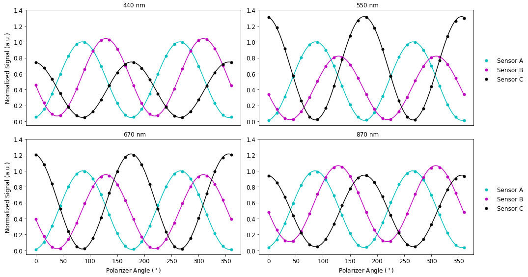
Figure 6 Malus curves for each of the four AirHARP channels. Each plot corresponds to an AirHARP channel, with data from Sensors A (cyan), B (magenta), and C (black) fit to Eq. (12) (solid lines). The data and fits are normalized to the Sensor A maximum and represent the closest 4 × 10 nadir pixel bin, in each channel, to the AirHARP optical axis. Note that the polarizer rotation angle is offset by −90°, as shown.

The optical path from the HARP front lens to a single FPA creates a single partial polarizer (i.e., Eq. 9). Therefore, this test creates a two-polarizer system. Malus' law explains the observed counts at each detector as a function of ϑ. To account for the optical complexity of HARP, we use a general fit:

$$\begin{array}{}\text{(11)}& {\mathrm{DN}}_{\det X}^{\ast }\left(\mathit{\vartheta }\right)=\mathit{\alpha }{\cos }^{\mathrm{2}}\left[\mathit{\vartheta }-({\mathit{\vartheta }}_X-\mathit{\beta })\right]+\mathit{\gamma },\end{array}$$

where the shorter subscript det X represents the background, linearity, and flatfield-corrected counts in a single detector (i.e., X could be A, B, or C) during this test and α, β, and γ are fit parameters. ϑ_X is the nominal polarizer angle for a detector X, determined during AirHARP pre-assembly testing. Figure 6 shows examples of Malus curves and fits to Eq. (11) for the three detectors and four channels, using co-located Moxtek data along the AirHARP optical axis.

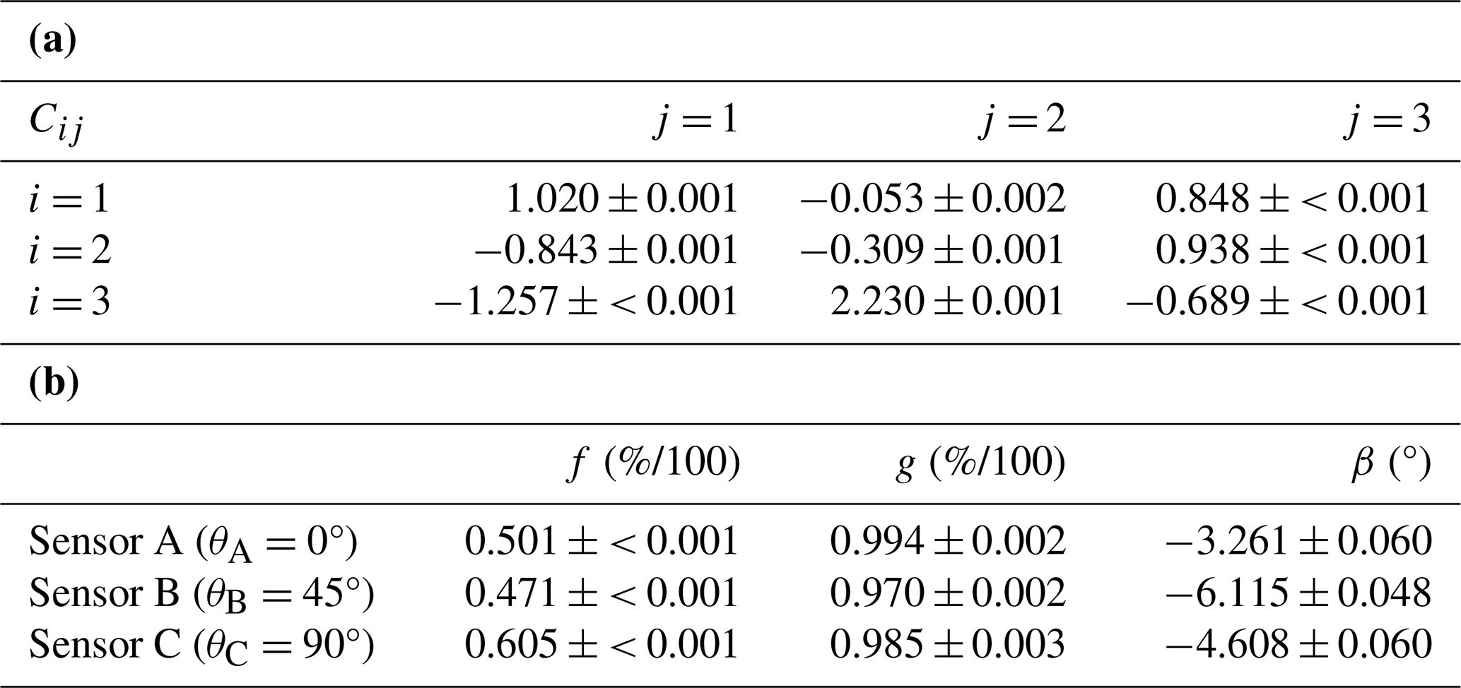
Table 2 (a) Example characteristic matrix elements, C_ij, for the 670 nm AirHARP band, via Eq. (12). (b) Example of instrument-relative parameters for the 670 nm AirHARP band, via Eq. (13).

The amplitude of the curves is related to the α and γ parameters, the phase to β, and the extinction (“lift” off the zero line) to γ. Any global bias due to the Moxtek polarizer itself is negligible or removable for the reasons stated above. Surface inhomogeneities on the polarizer may impart higher-order frequencies in the signal, which can be accounted for by Fourier decomposition (Cairns et al., 1999). A separate sensitivity study using a reference polarimeter and a rotating polarizer in our laboratory suggests that Fourier modes at the 0.005 level (such as sin4ϑ) stem from surface variations and are removed during this analysis. After normalizing each Malus curve by the maximum of the curve in det A for each channel and detector and inverting the matrix in Eq. (10), we come to a final relationship that completely represents this step:

$$\begin{array}{}\text{(12)}& \begin{array}{rl}& {\left[\begin{array}{c}\mathrm{1}\\ -\cos \mathrm{2}\mathit{\vartheta }\\ \sin \mathrm{2}\mathit{\vartheta }\end{array}\right]}_{\mathrm{inc}}\\ & =\left[\begin{array}{ccc}{C}_{\mathrm{11},}& C_{\mathrm{12}}& C_{\mathrm{13}}\\ C_{\mathrm{21}}& C_{\mathrm{22}}& C_{\mathrm{23}}\\ C_{\mathrm{31}}& C_{\mathrm{32}}& C_{\mathrm{33}}\end{array}\right]\left[\begin{array}{c}{\mathrm{DN}}_{\det \mathrm{A}}^{\ast }\left(\mathit{\vartheta }\right)\\ {\mathrm{DN}}_{\det \mathrm{B}}^{\ast }\left(\mathit{\vartheta }\right)\\ {\mathrm{DN}}_{\det \mathrm{C}}^{\ast }\left(\mathit{\vartheta }\right)\end{array}\right]{\left(max\left({\mathrm{DN}}_{\det \mathrm{A}}^{\ast }\right(\mathit{\vartheta }\left)\right)\right)}^{-\mathrm{1}},\end{array}\end{array}$$

​​​​​​​where the Stokes parameters (I, Q, U) are replaced with their theoretical forms and the matrix $\mathbf{C}=({\mathbf{M}}^{\ast }{)}^{-\mathrm{1}}$ from Eq. (10). This C is defined in Fernandez-Borda et al. (2009) as the characteristic matrix. The C translates normalized, corrected detector counts to normalized Stokes parameters for pixels along the optical axis (though applicable to polarization measurements anywhere in the FOV). The C⁻¹ has an analytical form based on the angle of the polarizers used for the three detectors (Schott, 2009):

$$\begin{array}{}\text{(13)}& \begin{array}{rl}& {\mathbf{C}}^{-\mathrm{1}}\\ & =\left[\begin{array}{ccc}{f}_{\mathrm{A}}& f_{\mathrm{A}}{g}_{\mathrm{A}}\cos \mathrm{2}\left({\mathit{\theta }}_{\mathrm{A}}-{\mathit{\beta }}_{\mathrm{A}}\right)& f_{\mathrm{A}}{g}_{\mathrm{A}}\sin \mathrm{2}\left({\mathit{\theta }}_{\mathrm{A}}-{\mathit{\beta }}_{\mathrm{A}}\right)\\ f_{\mathrm{B}}& f_{\mathrm{B}}{g}_{\mathrm{B}}\cos \mathrm{2}({\mathit{\theta }}_{\mathrm{B}}-{\mathit{\beta }}_{\mathrm{B}})& f_{\mathrm{B}}{g}_{\mathrm{B}}\sin \mathrm{2}\left({\mathit{\theta }}_{\mathrm{B}}-{\mathit{\beta }}_{\mathrm{B}}\right)\\ f_{\mathrm{C}}& f_{\mathrm{C}}{g}_{\mathrm{C}}\cos \mathrm{2}({\mathit{\theta }}_{\mathrm{C}}-{\mathit{\beta }}_{\mathrm{C}})& f_{\mathrm{C}}{g}_{\mathrm{C}}\sin \mathrm{2}\left({\mathit{\theta }}_{\mathrm{C}}-{\mathit{\beta }}_{\mathrm{C}}\right)\end{array}\right].\end{array}\end{array}$$

The coefficients define the transmission of the light through the entire optical system (f_X), polarizing efficiency (g_X), and phase offset (β_X) relative to the nominal detector polarizer angles (θ_X) from Eq. (11). This characteristic matrix can be solved in two ways: a least-squares approach in Eq. (12) using data from at least three Moxtek polarizer angles or a similar least-squares approach in the inverse matrix in Eq. (13). We prefer the former in this study, but consistency checks with the latter are useful. Table 2a gives the characteristic matrix coefficients with relative uncertainties using the least-squares method, and Table 2b gives example values with uncertainties using the parametric method. Both tables shown below represent a 4 × 4 nadir pixel bin for the 670 nm channel for AirHARP.

Table 2b shows that the nominal AirHARP polarizer angles (θ_X) can deviate from their derived values (β_X). Note that θ_X−β_X is the perceived polarization orientation of the entire light path from the perspective of each FPA. Retardances induced by the prism and/or detector polarizer will contribute to β_X. Note that the coefficients are significantly different from the Pickering matrix, the ideal matrix C for an AirHARP-like system (Schott, 2009). The characteristic matrix coefficients shown in Table 2a use the polarizer datasets alone, though current AirHARP L1B processing through Version 002 includes input from low-DOLP sources (integrating spheres, partial polarization generators) for closure in the entire DOLP range. The errors and values in Table 2a can be used to calculate the propagated uncertainty in the relative Stokes parameters, which is derived from Eq. (12):

$$\begin{array}{}\text{(14)}& \begin{array}{rl}{\mathit{\sigma }}_{S_i}^{\mathrm{2}}=& {\left(max\left({\mathrm{DN}}_{\det \mathrm{A}}^{\ast }\right(\mathit{\vartheta }\left)\right)\right)}^{-\mathrm{2}}\\ & \sum _{j=\mathrm{1}}^{\mathrm{3}}\left[{\left({\mathrm{DN}}_{\det j}^{\ast }{\mathit{\sigma }}_{C_{ij}}\right)}^{\mathrm{2}}+{\left(C_{ij}{\mathit{\sigma }}_{{\mathrm{DN}}_{\det j}^{\ast }}\right)}^{\mathrm{2}}\right],\end{array}\end{array}$$

where ${\mathit{\sigma }}_{S_i}$ is the standard deviation of the Stokes parameters (generally denoted by subscript S). We use the i iterant to define the Stokes parameter: [1, 2, 3] corresponds to [I, Q, U] and can be used interchangeably. ${\mathrm{DN}}_{\det j}^{\ast }$ is the result from Eq. (11), where the j iterant [1, 2, 3] corresponds to sensors [A, B, C]. ${\mathit{\sigma }}_{C_{ij}}$ is the uncertainty quoted in Table 2a for the C_ij matrix element, and ${\mathit{\sigma }}_{{\mathrm{DN}}_{\det j}^{\ast }}$ is the propagated uncertainty of the detector counts measurement. The value for ${\mathit{\sigma }}_{{\mathrm{DN}}_{\det j}^{\ast }}$ involves random elements such as shot, read, and dark-current noises and systematic elements from background, flatfield, and nonlinear correction. It may also include stray light and other noises that are difficult to decouple. At the integration times we use, shot noise and potentially scene spatial variability can dominate, so the standard deviation of data from a real AirHARP superpixel, i.e., a rectangular, connected set of along-track and cross-track pixels, is used.

3.5 Radiometric calibration

3.5.1 Relative spectral response

With the polarimetric calibration complete, the next step is radiometric calibration, which requires knowledge of spectral response. The AirHARP instrument uses several filters to define the four nominal wavelength channels, with bandwidths in parentheses: 440 nm (16 nm), 550 nm (13 nm), 670 nm (18 nm), and 870 nm (39 nm). The spectral response function (SRF) is defined by a multi-bandpass filter (MBPF) and the stripe filter on top of each detector.

To validate these filter specs, we placed the AirHARP instrument in the aperture of a separate 25.6 cm integrating sphere at NASA GSFC, fed by an Ekspla laser source. The Ekspla is a scanning monochromator capable of 1 nm precision over a 200–1000 nm range. We set the Ekspla source at a given wavelength and verified each output channel and bandwidth using an external Avantes spectrometer. We use the spectrometer output to correct the AirHARP measurements for any variation in Ekspla laser power over the course of the testing period.

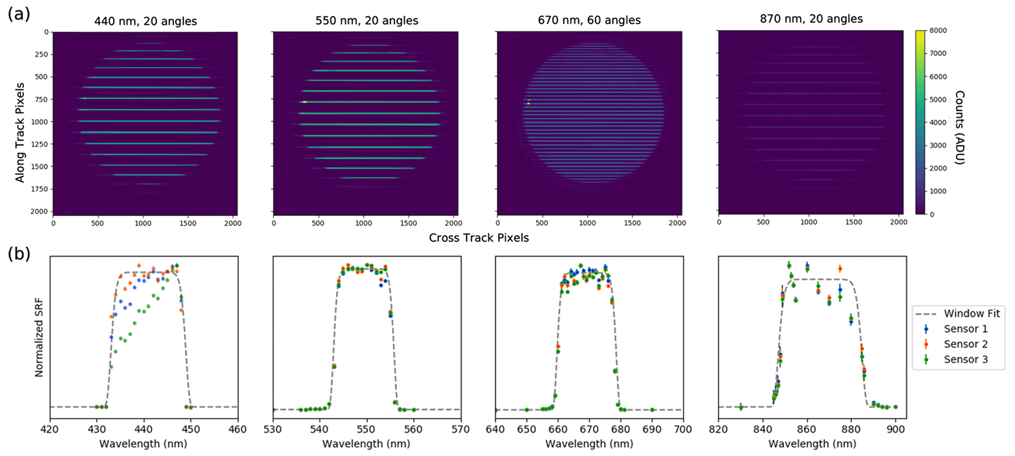
Figure 7 Examples of AirHARP images taken at different in-band Ekpsla wavelengths to show the distribution of illuminated stripes (a). The Ekspla power was weakest in the near-infrared, as evidenced in the 870 nm example ((a), right). The AirHARP SRF for the three sensors and the super-Gaussian SRF fit (gray) is shown in panel (b). The images in panel (b) correspond to the images in panel (a). All data shown in panel (b) are normalized to 1 for each channel and sensor individually.

The standard process is used in AirHARP images that are taken at each Ekspla wavelength setting. The Ekspla channels were chosen using a priori knowledge of the filter spectra from the manufacturer. A higher density of images was acquired in-band than out-of-band to capture the structure of the in-band SRF. Figure 7a shows AirHARP images of the integrating sphere, illuminated by four in-band Ekspla wavelengths. When the Ekspla is set to an in-band channel near 670 nm, the 60 AirHARP red view sectors are illuminated. For the other AirHARP channels, the sparser distribution of 20 view sectors appears whenever the Ekpsla is in-band. For Ekpsla wavelengths rejected by the AirHARP system, the images are compatible with the dark signal (Fig. 3b).

Using the telecentric technique, we take a small region of nadir pixels, correct their values via the process leading up to Eq. (4), and plot them against the Ekspla wavelength for a single HARP channel. Figure 7b shows the SRF for AirHARP Sensor 1 (blue dots), Sensor 2 (green dots), and Sensor 3 (orange dots) for 440 nm (left), 550 nm (left center), 670 nm (right center), and 870 nm (right). Because the SRF data are noisy, even after correction from an external spectrometer, we use a general super-Gaussian fit of order 6 (plotted in gray) to simplify the following analysis. Figure 7b also shows a differential SRF for the AirHARP 440 nm band, which is likely due to manufacturer error in the thin-film coating for the AirHARP prism interfaces or detector stripe filters. This 440 nm SRF differential is unique to AirHARP: we see no evidence of this in the HARP CubeSat or HARP2 440 nm designs (Sienkiewicz et al., 2024). We are pursuing several corrections for the AirHARP 440 nm spectral differential at the detector level and L1B stage, though further details are beyond the scope of this work.

This testing benefits two studies: (1) calculation of extraterrestrial solar irradiance used to convert radiance measured at the top of atmosphere (TOA) to reflectance (or the reflectance factor) and (2) radiometric calibration. To perform (1), we integrate the solar spectrum (here using the American Society for Testing and Materials Standard Extraterrestrial Spectrum Reference E-490 Air Mass Zero (AMZ) database (NREL, 2000) inside the SRF for each HARP wavelength):

$$\begin{array}{}\text{(15)}& F_{\mathrm{0}}\left(\mathit{\lambda }\right)={\displaystyle \frac{\mathrm{1}}{\mathrm{\Delta }\mathit{\lambda }}}\underset{{\mathit{\lambda }}_i}{\overset{{\mathit{\lambda }}_f}{\int }}B\left(\mathit{\lambda }\right)\mathrm{SRF}\left(\mathit{\lambda }\right)\mathrm{d}\mathit{\lambda },\end{array}$$

where λ is the wavelength (subscripts i and f denoting the shorter- and longer-wavelength edges of the spectral band; nm), Δλ is the bandwidth (nm), B(λ) is the solar spectral irradiance (W m⁻² nm⁻¹), and SRF(λ) is the spectral response function. We only use the structure of the in-band channel in Eq. (15) and fit each window to a sixth-order super-Gaussian function, due to unexplained noise in the dataset being larger than the uncertainty of each data point (especially at 870 nm). Normalized out-of-band rejection is at or below 0.001 for the 300 to 1050 nm range as well. Analysis of the second-order in-band differences relative to this theoretical fitting is ongoing but is not expected to contribute significantly to the L1B data product (AirHARP 440 nm notwithstanding). Table 3 shows the details of our spectral response testing and the extraterrestrial solar irradiance, F₀, calculated using Eq. (16), for each channel.

Table 3 Derived AirHARP parameters from spectral response analysis.

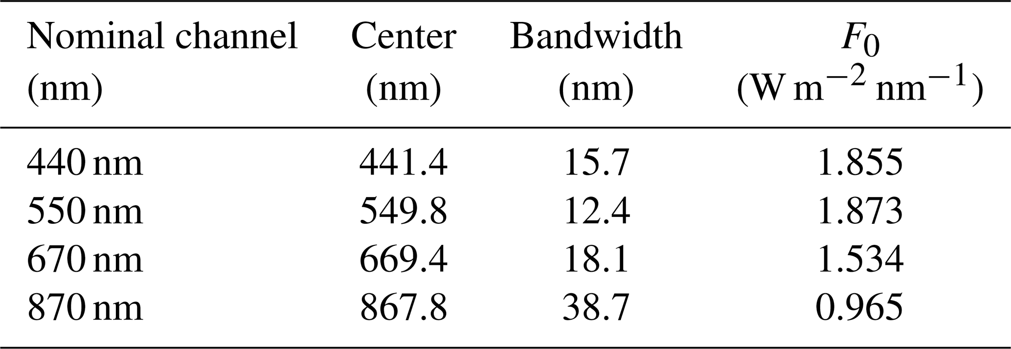
The final column of this chart is used to convert measured radiances to the reflectance factor as per

$$\begin{array}{}\text{(16)}& \mathit{\rho }\left(\mathit{\lambda }\right)={\displaystyle \frac{\mathit{\pi }L\left(\mathit{\lambda }\right)}{F_{\mathrm{0}}\left(\mathit{\lambda }\right)}},\end{array}$$

where ρ(λ) is the reflectance factor and L(λ) is the radiance (W m⁻² nm⁻¹ sr⁻¹), assuming a Lambertian scattering distribution of light in the pixel. We can divide Eq. (16) by the cosine of the solar zenith angle converted to TOA reflectance.

3.5.2 Gain characterization

Our radiometric calibration translates the normalized Stokes parameters into calibrated radiances (W m⁻² nm⁻¹ sr⁻¹). This step gives scientific weight to our measurements and allows us to retrieve radiative properties of the atmosphere and surface. Again, integrating spheres are optimal for this testing. For example, the radiometrically calibrated NASA GSFC Grande sphere is traceable to the National Institute of Standards and Technology (NIST), with calibration uncertainties publicly available for a comparable sphere (Cooper and Butler, 2020). The spectral sensitivity of Grande peaks around 1 µm, and each of the nine lamps adds linearly to the total illumination.

We set the AirHARP instrument under the same conditions as the polarimetric calibration discussed in Sect. 3.4.2, except with no polarizing element between the instrument and the integrating sphere. Because the lamps are incandescent sources, we adjust the AirHARP detector integration times to capture enough signal in the blue channel and stay out of saturation in the NIR. The standard process is used at each lamp level to create template images. Using the telecentric technique, we select a small nadir pixel bin for a given wavelength, correct the values using the process leading up to Eq. (4), and apply the characteristic matrix for that channel to the co-located data in each detector. The sphere output is depolarized, so the resulting Stokes parameters Q and U are statistically zero and the total intensity, I, contains all the information content. As per Eq. (12), the resulting I is in counts but represents the band-weighted signal measured by a particular AirHARP channel. To find the equivalent radiance levels as observed by AirHARP, the solar spectrum, B(λ), is replaced by the Grande SRF in Eq. (15) (Cooper and Butler, 2020), and this calculation is performed for each lamp and wavelength. The radiometric calibration derives the slope (W m⁻² nm⁻¹ sr⁻¹ ADU⁻¹) that translates the normalized AirHARP intensities to the calibrated radiances:

$$\begin{array}{}\text{(17)}& \begin{array}{rl}{L}_{\mathrm{lamp}}& =k\left(C_{\mathrm{11}}{\mathrm{DN}}_{\det \mathrm{A}}^{\ast }+C_{\mathrm{12}}{\mathrm{DN}}_{\det \mathrm{B}}^{\ast }+C_{\mathrm{13}}{\mathrm{DN}}_{\det \mathrm{C}}^{\ast }\right)\\ & +\mathit{ϵ},\end{array}\end{array}$$

where L_lamp is the calibrated radiance (W m⁻² nm⁻¹ sr⁻¹) at that lamp level. The parameter k is our gain factor, and ϵ is a linear bias. For all the channels, the linear bias ϵ is compatible with zero within 3 standard deviations of the least-squares fit error in this coefficient. Therefore, the general calibration equation for the AirHARP instrument is the following:

$$\begin{array}{}\text{(18)}& \left[\begin{array}{c}I\\ Q\\ U\end{array}\right]=k\left[\begin{array}{ccc}{C}_{\mathrm{11}}& C_{\mathrm{12}}& C_{\mathrm{13}}\\ C_{\mathrm{21}}& C_{\mathrm{22}}& C_{\mathrm{23}}\\ C_{\mathrm{31}}& C_{\mathrm{32}}& C_{\mathrm{33}}\end{array}\right]\left[\begin{array}{c}{\mathrm{DN}}_{\det \mathrm{A}}^{\ast }\\ {\mathrm{DN}}_{\det \mathrm{B}}^{\ast }\\ {\mathrm{DN}}_{\det \mathrm{C}}^{\ast }\end{array}\right],\end{array}$$

and the complete, propagated uncertainty of the L1B calibrated radiances is

$$\begin{array}{}\text{(19)}& \begin{array}{rl}{\mathit{\sigma }}_{S_i}^{\mathrm{2}}& =\sum _{j=\mathrm{1}}^{\mathrm{3}}{k}^{\mathrm{2}}\left[{\left({\mathrm{DN}}_{\det j}^{\ast }{\mathit{\sigma }}_{C_{ij}}\right)}^{\mathrm{2}}+{\left(C_{ij}{\mathit{\sigma }}_{{\mathrm{DN}}_{\det j}^{\ast }}\right)}^{\mathrm{2}}\right]\\ & +{\left(C_{ij}{\mathrm{DN}}_{\det j}^{\ast }{\mathit{\sigma }}_k\right)}^{\mathrm{2}},\end{array}\end{array}$$

where the subscripts follow the same convention as Eq. (14).

4 Validation of calibrated measurements

4.1 Nadir coefficients

Before we evaluate the calibration over the entire FOV, it is important that we validate the same lens locations that we used to calibrate the instrument. Here, we evaluate the nadir coefficients for a range of partially polarized DOLP signals, like those AirHARP observes in field data.

In the atmosphere, DOLP measurements close to 1 occur only at certain geometries with sunglint over the dark ocean or Rayleigh scattering in the ultraviolet. More often, a complex atmosphere–land–ocean scene generates partially polarized light (0 < DOLP < 1). To simulate this, a partial polarization generator box (POLBOX), a Fresnel device comprised of two rotatable glass blades with an equal index of refraction, is used (Fig. 8a). This polarization state generator is widely used for laboratory validation of spaceborne polarimeters (van Harten et al., 2018; Li et al., 2018; Smit et al., 2019). Any deviation in the DOLP retrieval gives the laboratory calibration uncertainty of the HARP system after systematic POLBOX uncertainty is accounted for. The POLBOX DOLP is analytic, and the values for each blade setting can be determined by the sequential Fresnel interactions at each air–glass interface:

$$\begin{array}{}\text{(20)}& {\mathrm{DoLP}}_{\mathrm{POLBOX}}={\displaystyle \frac{\begin{array}{c}\mathit{\alpha }\left(n,\mathit{\lambda }\right){\cos }^{\mathrm{2}}\left(\mathrm{2}\mathit{\theta }\right)+\mathit{\beta }\left(n,\mathit{\lambda }\right)\cos \left(\mathrm{2}\mathit{\theta }\right)\\ +\mathit{\gamma }\left(n,\mathit{\lambda }\right)\end{array}}{\begin{array}{c}\mathit{\epsilon }\left(n,\mathit{\lambda }\right){\cos }^{\mathrm{2}}\left(\mathrm{2}\mathit{\theta }\right)+\mathit{\mu }\left(n,\mathit{\lambda }\right)\cos \left(\mathrm{2}\mathit{\theta }\right)\\ +\mathit{\omega }\left(n,\mathit{\lambda }\right)\end{array}}},\end{array}$$

where α, β, γ, ε, μ, and ω are glass-specific coefficients dependent on the refractive index n and the wavelength λ, and θ is the glass blade angle. For our test, we keep the POLBOX glass blades perpendicular to the table and take HARP images at increasing blade angles. The angle of the blades is controlled with a fine micrometer dial, and the angle is known within 0.25°. The data are corrected through the process leading up to Eq. (4), and the precomputed calibration matrices are applied for each wavelength and image in the dataset. As mentioned above, the characteristic matrix used in this validation includes Moxtek polarizer data and input Stokes vectors that represent unpolarized light for closure over the entire DOLP range. Using the same nadir pixel bin that was used for calibration, the measured Stokes parameters at each POLBOX blade angle are processed into the DOLP via Eq. (7) (neglecting V), and these results are compared to Eq. (20) for each blade angle and wavelength.

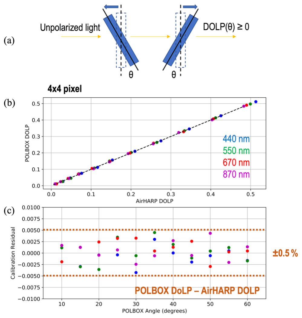
Figure 8 The POLBOX system generates partial polarization by rotating two glass blades (a). When comparing the DOLP theory to AirHARP measurement in all channels (b), we see that AirHARP reproduces the entire POLBOX range within ±0.5 % DOLP (c). The lamp reflectance for this measurement was > 0.09 in all channels.

The measured DOLP from the HARP system is within ±0.5 % (with a 1σ uncertainty of 0.25 % in DOLP) of the true POLBOX values for all wavelengths, given a 4 × 4 px nadir bin, as shown in Fig. 8b–c. Glass blade angles (< 5°) that create back-reflections in the wide HARP FOV are neglected in the comparison. Removing these angles has a negligible impact on the comparison, as the theoretical DOLP at 10° is still quite low (∼ 4 %) and still represents a depolarized environment. The POLBOX itself imparts a static DOLP uncertainty of 0.0015 related to the uncertainty in the glass blade angle (Li et al., 2018). This experiment is only limited by the intensity of the integrating sphere, which here was no less than 0.09 in reflectance (440 nm). This level is a bit higher than the typical aerosol signal used in theoretical experiments (L_typ), but it is challenging to balance integration time and saturation in a single laboratory measurement when all channels are simultaneously exposed. Even so, we conclude that the HARP design allows for a highly accurate pre-launch DOLP baseline for all channels relative to recommended cloud and aerosol science uncertainty benchmarks (NASA, 2015, 2021). A limited error model is given in Appendix B, and a comprehensive version is anticipated in future work.

4.2 Full-FOV intercomparisons with field data

4.2.1 AirHARP participation in the ACEPOL campaign

Sensitivity tests in the laboratory allow us to characterize the HARP instrument in a well-controlled setting. However, these environments can be limited by resources and time, and this can impact how much of the FOV, spectral channels, and dynamic range are characterized. To validate the full-FOV calibration, we take field data and compare how the HARP instrument measures the multi-angle reflectance factor and polarized signal with a similar MAP over a common target.

AirHARP participated in two NASA aircraft campaigns in 2017: LMOS (Stanier et al., 2021) and ACEPOL (Knobelspiesse et al., 2020). LMOS took place over Lake Michigan and eastern Wisconsin from 25 May to 19 June 2017 and ACEPOL over the southwestern United States and eastern Pacific Ocean from 23 October to 9 November 2017. LMOS was AirHARP's debut and was the only instrument of its kind taking measurements during this period. ACEPOL, on the other hand, included two lidar and four polarimeter instruments on the aircraft, including AirHARP. A major goal of the ACEPOL campaign was to compare different polarimeter concepts over common targets, improve cross-calibration studies, and develop new synergistic algorithms for retrieving aerosol, cloud, land, and ocean properties.

During ACEPOL, these six instruments observed over 30 scenes, including urban cities, coastal oceans, dry lakes, cloud decks, and prescribed wildfire smoke. Two of these targets are best suited for reflective solar band calibration and validation: sunglint over the dark ocean and the Rosamond Dry Lake, a flat desert site in California. Sunglint is highly polarized at some geometries, reaching a DOLP of nearly 1 in the optical regime. Off-glint, polarization is reduced and low ocean albedo is useful for validating dim reflectances. The sunglint signal can be modeled accurately if the viewing and solar geometries are known and aerosol and Rayleigh scattering are removed. The appearance of sunglint depends on the ocean surface wind speed, which can roughen the surface and break up the signal (Cox and Munk, 1954). Despite strong surface winds, the ocean surface is considered flat from a viewing altitude of 20 km and requires no special topography correction to the data. Multi-angle polarimeters, like AirHARP, measure the way the sunglint signal varies with the viewing angle and can reproduce a discrete intensity and polarization profile with the angle. Therefore, sunglint datasets are very convenient for use in calibration validation. The Rosamond Dry Lake is also a useful calibration target: it is a pseudo-invariant, highly reflective surface with a low-DOLP profile. We use several ACEPOL ocean and desert datasets as a limited demonstration that our telecentric technique captures the expected performance of the AirHARP instrument across the FOV.

Because the focus of this work is calibration and not data intercomparisons, we will present the following section in a simple and limited sense. The RSP instrument was chosen as our validator because it best matches the along-track angular sampling of HARP, shared the same wing of ER-2 with AirHARP during ACEPOL, and has the longest history of accurate, validated polarimetric measurements. The following describes the process used to co-locate AirHARP and RSP measurements at similar viewing angles.

1. A target of interest and a reference lat–long pair are identified, and the closest scan in the RSP data is found. The average lat–long pair of this scan becomes the new reference lat–long point.

2. The algorithm finds the closest matching view zenith angle (VZA) and view azimuth angle (VAA) between AirHARP and the RSP over this common target. The search yields a successful match if the VZA difference is < 1° and the VAA difference is < 5°.

3. The lat–long coordinate of the matching RSP measurement is now the updated lat–long point for comparison.

4. A spatial mask that accounts for the 220 m RSP footprint and smear profile (Knobelspiesse et al., 2019) is applied to the AirHARP pixels around this lat–long point. The resulting spatially weighted mean and standard deviations for the VZA, VAA, solar azimuth (SAA) and zenith (SZA), I, Q, U, and DOLP are logged for AirHARP and the matching respective values for the RSP.

5. This process is repeated for all relevant spectral channels.

The intercomparison is validated using an error-normalized difference in both reflectance and DOLP for the three shared channels individually. We use the error models for both AirHARP and the RSP (see the Appendices) to study how well their measurements agree within their mutual uncertainty. Similar work in multi-angle polarimetric intercomparisons was done in Knobelspiesse et al. (2019). The following is our metric:

$$\begin{array}{}\text{(21)}& \mathit{\chi }={\displaystyle \frac{{\mathit{\rho }}_{\mathrm{AirHARP}}-{\mathit{\rho }}_{\mathrm{RSP}}}{\sqrt{{\mathit{\sigma }}_{\mathit{\rho },\mathrm{AirHARP}}^{\mathrm{2}}+{\mathit{\sigma }}_{\mathit{\rho },\mathrm{RSP}}^{\mathrm{2}}}}},\end{array}$$

where ρ is the reflectance measurement and σ_ρ is the 1σ reflectance uncertainty. Equation (21) will be used similarly for DOLP measurements. If the error models adequately describe the measurement, we expect the residuals normalized by their uncertainties to have a normal distribution. In other words, if 68.27 % (95.45 %) of the Eq. (21) results lie in the range ±1 (±2), this suggests statistical agreement. This also suggests that the AirHARP calibration can sufficiently reproduce the reflectance and DOLP of Earth scenes relative to a similar, co-located multi-angle polarimeter. The following will discuss the results of the AirHARP and RSP intercomparison over both ocean and desert sites during the ACEPOL campaign.

4.2.2 Results and discussion

The full-FOV comparison with the RSP uses two ocean cases from 23 October 2020 and five desert cases from 25 October 2020, taken during the ACEPOL campaign. The ocean captures occurred 30 min apart off the coast of California, the first at 20:10 UTC over 35.12° N, 124.75° W and the second at 20:49 UTC over 31.75° N, 122.38° W. We will identify the former as Ocean 1 and the latter as Ocean 2 going forward, and both are parallel to and slightly off the solar principal plane. The five desert cases were taken on 25 October 2020 over the Rosamond Dry Lake site in California, also 30 min apart: 17:28, 17:55, 18:26, 18:55, and 19:28 UTC. These captures will be identified as Desert 1 through 5, respectively, and all targeted the general region around 34.83° N, 118.07° W.

The AirHARP and RSP data were ordered for these dates, times, and locations, and the co-location procedure described in Sect. 3.2.1 was followed for each of the sites and the three spectral channels common to both instruments: 550, 670, and 865 or 870 nm. We do not show a comparison with the AirHARP 440 nm band because there is no comparable RSP channel and, for the SRF, the reasons mentioned above could complicate the interpretation of the results. The AirHARP 550 nm (13 nm), 670 nm (18 nm), and 870 nm (39 nm) and RSP 550 nm (20 nm), 670 nm (20 nm), and 865 nm (20 nm) spectral bands are generally compatible. We also do not expect any significant differences in the signal of the desert or glint targets relative to SRF differences. We did not perform any spectral matching in this work.

Figure 9 shows a multi-angle comparison of AirHARP and the RSP for four of the seven ACEPOL datasets. RSP data are in black, together with the AirHARP desert (red) and ocean (blue) data for both the reflectance factor (first column, calculated with Eq. 17) and DOLP (second column). Three compatible channels are shown: 550 nm (top row), 670 nm (middle row), and 870 nm (bottom row). The error bar on the AirHARP points is the subpixel standard deviation of the superpixel at each angle. This figure was developed by searching for the closest match between AirHARP and the RSP reflectance factor and DOLP measurements over a similar view geometry. After all matches were found, the RSP data were interpolated to the AirHARP scattering angles. We can use Fig. 9 to explore the angular information content in both desert and ocean scenes. For the ocean cases, the reflectance factor is lower than 0.1 in all the channels, but the DOLP range is wide, 0 to ∼ 0.8. The desert cases were chosen specifically to contrast with sunglint. The desert cases shown in Fig. 9 also represent the same target viewed from two different headings. The dependency on viewing geometry is clear in the separation of the desert reflectance factor curves in all the channels. These cases provide a range of geometries for intercomparison and adequate contrast in the reflectance factor and DOLP to validate our calibration.

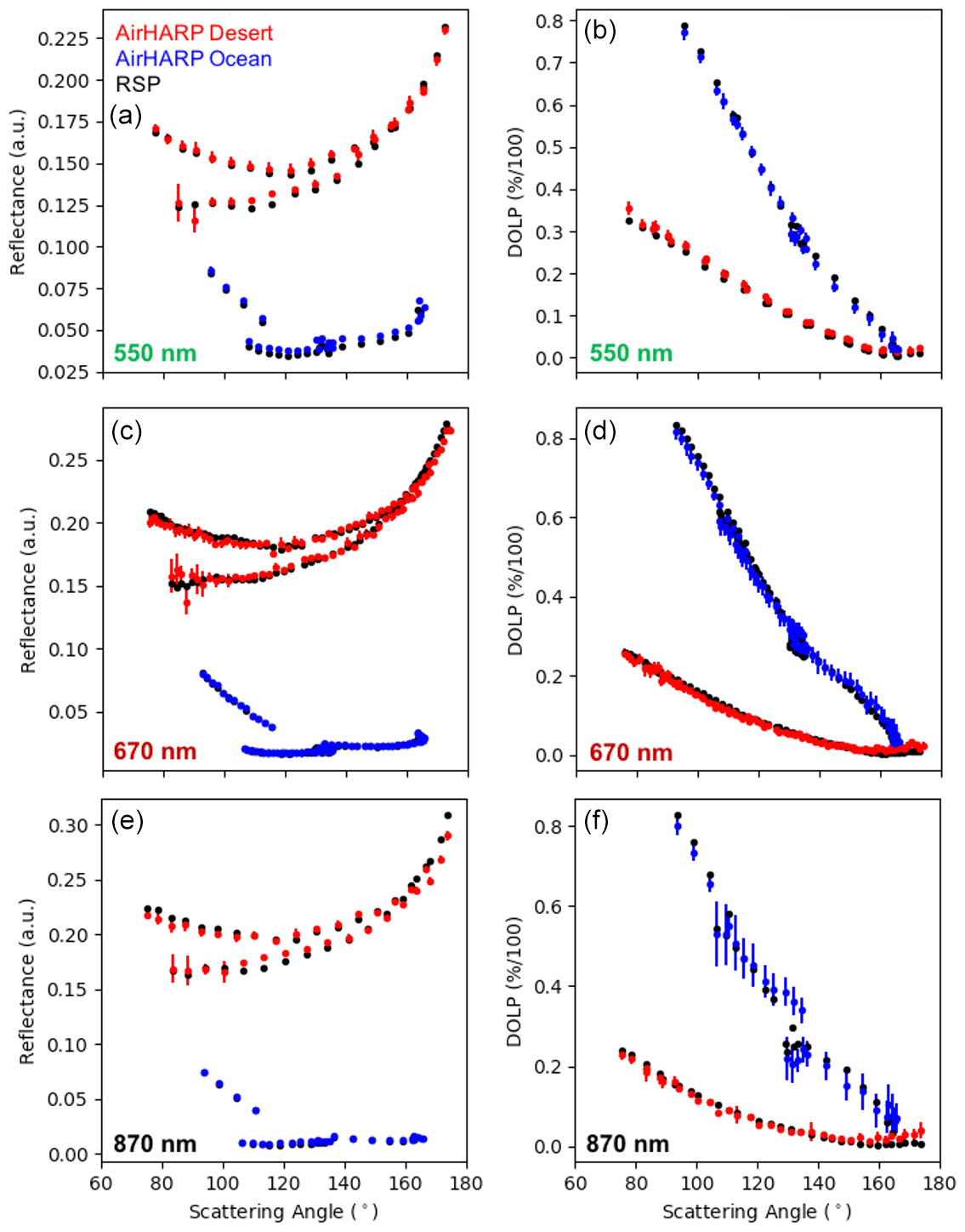
Figure 9 Multi-angle, interpolated matchups between AirHARP and the RSP for ACEPOL targets. The reflectance factor (a, c, e) and DOLP (b, d, f) are compared for three compatible spectral channels: 550 nm (a, b), 670 nm (c, d), and 870 nm (e, f). AirHARP data in the colors and the RSP are black, with red signifying Desert 1 and Desert 2 cases and blue Ocean 1 and Ocean 2 cases. Error bars in the AirHARP data represent the standard deviation of the superpixel bin.

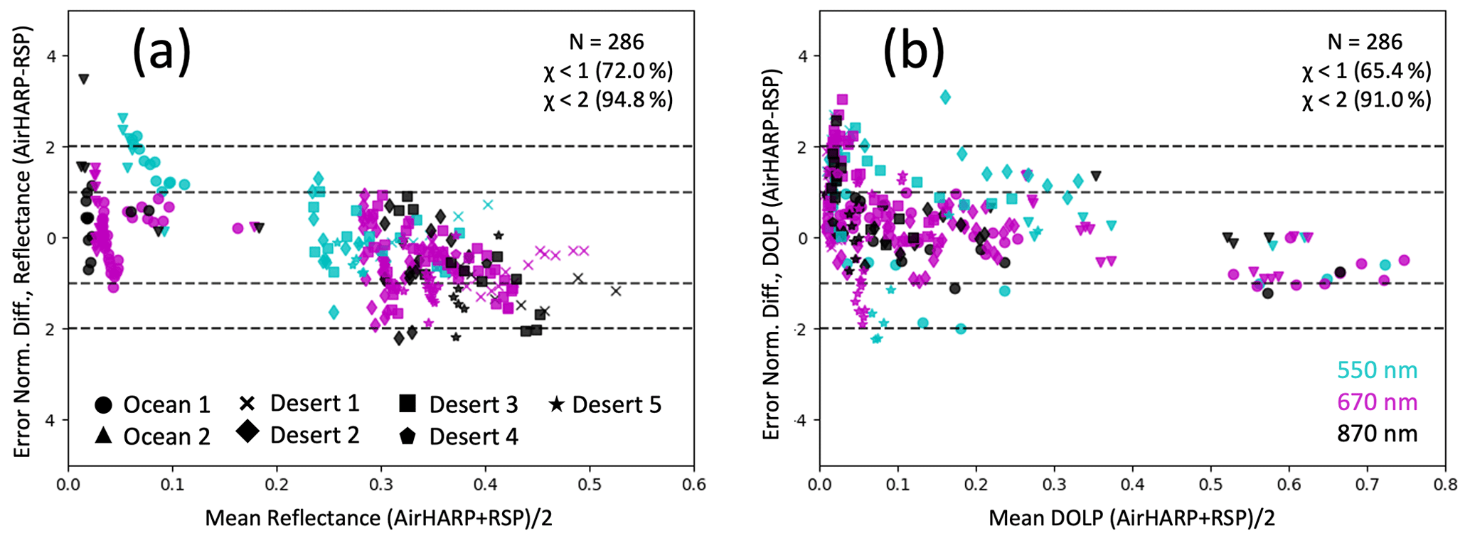
Figure 10 Error-normalized difference comparison between AirHARP and RSP reflectance (a) and DOLP (b) for 550 nm (cyan), 670 nm (magenta), and 870 nm (black) data over two ocean and five desert ACEPOL cases (markers). The dashed black lines represent boundaries where the residuals are 1 and 2 times the mutual uncertainty of the AirHARP and RSP error models. All data shown represent co-located angular matchups within 1° VZA and 5° VAA. Only data with VZA ≤ 35° are shown.

The following is a more rigorous intercomparison. Figure 10 shows the error-normalized differences from the direct angle-to-angle, filtered matchups in reflectance (Fig. 10a, not a reflectance factor) and DOLP (Fig. 10b) taken by AirHARP and the RSP across the seven datasets. Colored points are the relevant channels (550 nm in cyan, 670 nm in magenta, and 870 nm in black), and the markers denote the different datasets. Across the three channels and scenes, we see that, for reflectance, 72.0 % of the 286 filtered data points lie within ±1 and 94.8 % within ±2. For DOLP, those numbers are similar: 65 % and 91.0 %. The ideals are 68.27 % and 95.45 % for a normally distributed error residual. This suggests that the mutual uncertainty reasonably describes the variance between AirHARP and the RSP and that their measurements are generally compatible. There are some interesting features to note. The weak downward trend in reflectance suggests that the error models may diverge for reflectances beyond 0.5. However, nearly all data in the 0.2–0.5 reflectance range are desert matchups, and those cases may differ from ocean observations for a variety of reasons. The 550 nm comparison in DOLP (cyan, Fig. 10b) also shows more scatter relative to 670 and 870 nm. These features may also be an artifact of a limited scene sample size, so a larger intercomparison study would be useful. It is also important to note that this comparison only includes matchups with VZA ≤ 35° to limit pointing knowledge, georegistration, and pixel projection errors in the comparison.

However, some errors may still exist. During ACEPOL, AirHARP did not have an onboard calibrator, mechanism of temperature regulation, or dry purge. If the field measurement was impacted by ascent–descent humidity changes, differences in temperature between the aircraft pod and the outside environment, or condensation of water and aggregation of ice particles on the front lens, these effects may be difficult to characterize. These may have asymmetric impacts on the data at different FOVs as well.

In Fig. 9, we see some deviations between the AirHARP-RSP measurements, especially at larger scattering angles at 670 and 870 nm. This deviation may also be connected to georegistration at the widest angles, any unaccounted-for misregistration between the RSP and AirHARP, and/or interpolation at the AirHARP L1B stage. The HARP front lens distorts the ground projection by a factor of 4 at the furthest angles relative to the nadir, so the amount of interpolation needed to fit the data on a common L1B grid is much more intense at far angles. This is complicated by “pitch surfing” of ER-2. In several cases during ACEPOL, ER-2 hit slight turbulence during flight, which briefly tilted the AirHARP instrument off-nadir. Pitch surfing may grow the pixel projection at far angles and adds uncertainty to our interpolation of these angles at the gridding stage.

However, the overall structure of the RSP signal is reproduced by the AirHARP instrument across two different scenes, in a wide range of view angles, and relative to their mutual uncertainty. These results show the strength of our simple and efficient telecentric technique. The accuracy of this calibration is indirectly demonstrated in AirHARP Level-2 aerosol and cloud retrieval studies in Puthukuddy et al. (2020) and McBride et al. (2020) as well. Both studies use full-FOV datasets.

It is also important to note that cross-validation between instruments cannot determine which instrument is “more correct”, only how well they both agree over a common range of angles, channels, and targets. The community anticipates a third-party intercomparison study in the future that will compare the measurements of all ACEPOL polarimeters with each other, vector radiative transfer models, and other co-located satellite instruments.

5 Conclusions

The AirHARP calibration pipeline presented in this work exceeds the community requirement of 0.5 % DOLP in the laboratory and reproduces the signal of natural targets relative to another co-located polarimeter. The telecentric calibration scheme is as effective as it is simple. It is also possible in a variety of environments: in space, where physical access is impossible, and during field campaigns, where time and access to the instrument are limited. If a flatfield measurement is done regularly and consistently, the performance of the entire FPA can be traced through a range of temperatures and humidity environments (on aircraft). The HARP2 instrument on the NASA PACE mission includes an internal calibrator to validate the full-FOV performance throughout the life of the mission.

The telecentric technique can also be used for vicarious calibration with field data alone. In the laboratory calibration, we used a rotating polarizer–sphere setup and pixels at the center of the lens to calculate the characteristic matrix. This is a special case. In general, any polarized target viewed from at least three different angles may provide enough information to trend the characteristic matrix. It is important that the target is viewed from a significantly different geometry (optimally with views parallel and perpendicular to the solar plane and/or at least three attack angles 60° apart). This achieves the highest discrimination between polarization states (Tyo et al., 2006). Therefore, sunglint, cloudbow, dry lake, salt flat, aerosol plume, polar ice, and other natural targets can be excellent homogeneous and/or stable vicarious calibration targets. Measurements of these targets, combined with an internal flatfield measurement, may allow for effective and efficient trending of the instrument.

The telecentric technique can also be used to cross-calibrate HARP against other polarimetric instruments. For example, a direct intercomparison of AirHARP and the RSP could be used to derive a radiometric correction factor that could be applied to the characteristic matrix in Eq. (18). Because the radiometric k-factor applies to the entire matrix, a single co-located intercomparison between similar instruments is enough to correct the measurement. Using co-located instruments in this way also transfers their uncertainty in geolocation, measurement accuracy, and pointing. Nevertheless, it is invaluable over ill-modeled targets and/or for validation against solar or lunar views. The HARP science team is currently evaluating how this telecentric technique can improve the in-flight calibration of AirHARP and HARP CubeSat data. We anticipate that these methods will be applied to and expanded with HARP2 in 2024 and beyond.

Appendix A: RSP error model

The RSP error model is provided in Knobelspiesse (2015). The overall error in reflectance and DOLP is described below:

$$\begin{array}{}\text{(A1)}& {\displaystyle }{\mathit{\sigma }}_{\mathit{\rho }}^{\mathrm{2}}={\left({\displaystyle \frac{r^{\mathrm{2}}{\mathit{\sigma }}_{\mathrm{floor}}}{{\mathit{\mu }}_{\mathrm{s}}}}\right)}^{\mathrm{2}}+{\displaystyle \frac{a{R}_I{r}^{\mathrm{2}}}{{\mathit{\mu }}_{\mathrm{s}}}}+{\displaystyle \frac{{\mathit{\sigma }}_{\ln K}^{\mathrm{2}}{R}_P^{\mathrm{2}}}{\mathrm{16}}}+{\mathit{\sigma }}_{a_{\mathrm{c}}}^{\mathrm{2}}{R}_I^{\mathrm{2}},\text{(A2)}& {\displaystyle }\begin{array}{rl}{\mathit{\sigma }}_{\mathrm{DOLP}}^{\mathrm{2}}\left(\mathrm{noise}\right)& =\mathrm{4}\left(\mathrm{1}+{\displaystyle \frac{{\mathrm{DOLP}}^{\mathrm{2}}}{\mathrm{2}}}\right){\left({\displaystyle \frac{r^{\mathrm{2}}{\mathit{\sigma }}_{\mathrm{floor}}}{{\mathit{\mu }}_{\mathrm{s}}{R}_I}}\right)}^{\mathrm{2}}\\ & +\mathrm{2}\left(\mathrm{1}-{\displaystyle \frac{{\mathrm{DOLP}}^{\mathrm{2}}}{\mathrm{2}}}\right)\left({\displaystyle \frac{a{r}^{\mathrm{2}}}{{\mathit{\mu }}_{\mathrm{s}}{R}_I}}\right),\end{array}\text{(A3)}& {\displaystyle }\begin{array}{rl}{\mathit{\sigma }}_{\mathrm{DOLP}}^{\mathrm{2}}\left(\mathrm{cal}\right)& ={\displaystyle \frac{{\mathit{\sigma }}_{\ln K}^{\mathrm{2}}}{\mathrm{2}}}\left[\mathrm{1}-{\mathrm{DOLP}}^{\mathrm{2}}\right.\\ & \left.+{\displaystyle \frac{{\mathrm{DOLP}}^{\mathrm{4}}}{\mathrm{2}}}\left(\mathrm{1}-{\displaystyle \frac{\mathrm{1}}{\mathrm{2}}}{\sin }^{\mathrm{2}}\mathrm{4}\mathit{\chi }\right)\right],\\ & +{\mathit{\sigma }}_{\ln a}^{\mathrm{2}}{\mathrm{DOLP}}^{\mathrm{2}}\end{array}\text{(A4)}& {\displaystyle }{\mathit{\sigma }}_{\mathrm{DOLP}}^{\mathrm{2}}={\mathit{\sigma }}_{\mathrm{DOLP}}^{\mathrm{2}}\left(\mathrm{noise}\right)+{\mathit{\sigma }}_{\mathrm{DOLP}}^{\mathrm{2}}\left(\mathrm{cal}\right).\end{array}$$

Several parameters are prescribed, based on Knobelspiesse (2015):

• solar distance (au), r: 1;

• noise floor, σ_floor (× 10⁻⁵): 2.5 (550 nm), 2.2 (670 nm), and 2.0 (865 nm);

• shot noise parameter, a (× 10⁻⁹): 4.5 (550 nm), 3.7 (670 nm), and 3.7 (865 nm);

• relative gain coefficient cal uncertainty, σ_ln K: 0.005;

• absolute radiometric uncertainty, ${\mathit{\sigma }}_{a_{\mathrm{c}}}$: 0.03; and

• polarimetric characterization uncertainty, σ_ln a: 0.001.

Other parameters are given in the field datasets and are a function of observational geometry and the Earth scene:

• cosine of the solar zenith angle μ_s;

• intensity reflectance R_I;

• polarized reflectance R_P; and

• DOLP.

Finally, the RSP DOLP uncertainty depends on the angle of polarization, χ, in Eq. (A3). In a sensitivity study with the above parameters and field data, we found that the intercomparison with AirHARP did not vary meaningfully when χ varied between 0 and 180°. Therefore, sin ²4χ was set to its expectation value, 0.5, which represents any angle $\mathit{\chi }=(\mathrm{45}n+\mathrm{11.25})$° for n in Z.

Appendix B: AirHARP error model

The error model for AirHARP follows detector noises and systematics all the way to the Stokes parameters using Eqs. (18) and (19). Using Eq. (19) with i = 1 and rearranging the numerator, we show the radiance (or reflectance, via conversion) calibration and noise uncertainty:

$$\begin{array}{}\text{(B1)}& {\left({\displaystyle \frac{{\mathit{\sigma }}_I}{I}}\right)}^{\mathrm{2}}={\displaystyle \frac{\begin{array}{c}{\sum }_{j=\mathrm{1}}^{\mathrm{3}}{\mathrm{DN}}_{\det j}^{\ast \mathrm{2}}\left[{\left(k{\mathit{\sigma }}_{{\mathrm{C}}_{\mathrm{1}\mathrm{j}}}\right)}^{\mathrm{2}}+{\left(C_{\mathrm{1}j}{\mathit{\sigma }}_k\right)}^{\mathrm{2}}\right]\\ +{\left(k{C}_{\mathrm{1}j}{\mathit{\sigma }}_{{\mathrm{DN}}_{\det j}^{\ast }}\right)}^{\mathrm{2}}\end{array}}{{\left(\sum _{j=\mathrm{1}}^{\mathrm{3}}k{C}_{\mathrm{1}j}{\mathrm{DN}}_{\det j}^{\ast }\right)}^{\mathrm{2}}}}.\end{array}$$

From Table 2b (AirHARP 670 nm), the matrix element error ${\mathit{\sigma }}_{C_{\mathrm{1}j}}$ is comparable for all the elements (∼ 1 × 10⁻³). The radiometric factor k is 1.47 × 10⁻⁵ W m⁻² nm⁻¹ sr⁻¹ ADU⁻¹, the radiometric uncertainty σ_k is 1 × 10⁻³ ⋅ k​​​​​​​, and the calibration matrix elements C_1j are 1.020, −0.053, and 0.848 for j = [1, 2, 3]. The ${\mathrm{DN}}_{\det j}^{\ast }$ is not part of the L1B product but can be retrieved using Eq. (18) in reverse. The ${\mathit{\sigma }}_{{\mathrm{DN}}_{\det j}^{\ast }}$ is a mixture of detector noises, calibration fit errors, pixel aggregation, and spatial variability in the scene. We typically approximate this as the standard deviation of the radiance in the L1B data, which is the main contributor to radiometric noise. The radiometric uncertainty in the L1B is thus

$$\begin{array}{}\text{(B2)}& {\left({\displaystyle \frac{{\mathrm{\Delta }}_R}{R}}\right)}^{\mathrm{2}}={\left(\mathrm{0.03}\right)}^{\mathrm{2}}+{\left({\displaystyle \frac{{\mathit{\sigma }}_I}{I}}\right)}^{\mathrm{2}},\end{array}$$

where the first term accounts for the transfer radiometry error from integrating spheres, and the second term addresses the superpixel SNR (using the radiance product, I, from the L1B granule). The AirHARP DOLP uncertainty is a propagation from Eq. (7):

$$\begin{array}{}\text{(B3)}& {\mathit{\sigma }}_{\mathrm{DOLP}}^{\mathrm{2}}=\left({\displaystyle \frac{Q^{\mathrm{2}}{\mathit{\sigma }}_Q^{\mathrm{2}}+U^{\mathrm{2}}{\mathit{\sigma }}_U^{\mathrm{2}}}{I^{\mathrm{2}}(Q^{\mathrm{2}}+U^{\mathrm{2}})}}\right)+{\left(-{\displaystyle \frac{\sqrt{Q^{\mathrm{2}}+U^{\mathrm{2}}}}{I^{\mathrm{2}}}}{\mathit{\sigma }}_I\right)}^{\mathrm{2}}.\end{array}$$

We can simplify using Eq. (7) again:

$$\begin{array}{}\text{(B4)}& \begin{array}{rl}{\mathrm{\Delta }}_{\mathrm{DOLP}}^{\mathrm{2}}& ={\left(\mathrm{0.0025}\right)}^{\mathrm{2}}+\left({\displaystyle \frac{Q^{\mathrm{2}}{\mathit{\sigma }}_Q^{\mathrm{2}}+U^{\mathrm{2}}{\mathit{\sigma }}_U^{\mathrm{2}}}{I^{\mathrm{4}}{\mathrm{DOLP}}^{\mathrm{2}}}}\right)\\ & +{\left(\mathrm{DOLP}{\displaystyle \frac{{\mathit{\sigma }}_I}{I}}\right)}^{\mathrm{2}},\end{array}\end{array}$$

where 0.0025 is a systematic offset from the POLBOX measurements (Fig. 8) and the last two terms are from Eq. (B3). We anticipate using an expanded set of characterization measurements from HARP2, detailed in Sienkiewicz et al. (2024), to develop a model that characterizes the entire FOV in this year.

In all the above equations, σ is the standard deviation of the radiance in the AirHARP superpixel (for I, Q, or U, as noted), which is weighted by the spatial mask.