Intercomparison of fast airborne ozone instruments to measure eddy covariance fluxes: spatial variability in deposition at the ocean surface and evidence for cloud processing

The air–sea exchange of ozone (O₃) is controlled by chemistry involving halogens, dissolved organic carbon, and sulfur in the sea surface microlayer. Calculations also indicate faster ozone photolysis at aqueous surfaces, but the role of clouds as an ozone sink is currently not well established. Fast-response ozone sensors offer opportunities to measure eddy covariance (EC) ozone fluxes in the marine boundary layer. However, intercomparisons of fast airborne O₃ sensors and EC O₃ fluxes measured on aircraft have not been conducted before. In April 2022, the Technological Innovation Into Iodine and GV Environmental Research (TI³GER) field campaign deployed three fast ozone sensors (gas chemiluminescence and a combination of UV absorption with coumarin chemiluminescence detection, CID) together with a fast water vapor sensor and anemometer to study iodine chemistry in the troposphere and stratosphere over Colorado and over the Pacific Ocean near Hawaii and Alaska. Here, we present an instrument comparison between the NCAR Fast O₃ instrument (FO3, gas-phase CID) and two KIT Fast AIRborne Ozone instruments (FAIRO, UV absorption and coumarin CID). The sensors have comparable precision < 0.4 % Hz^−0.5 (0.15 ppbv Hz^−0.5), and ozone volume mixing ratios (VMRs) generally agreed within 2 % over a wide range of environmental conditions: 10 < O₃ < 1000 ppbv, below detection < NO_x < 7 ppbv, and 2 ppmv < H₂O < 4 % VMR. Both instrument designs are demonstrated to be suitable for EC flux measurements and were able to detect O₃ fluxes with exchange velocities (defined as positive for upward) as slow as −0.010 ± 0.004 cm s⁻¹, which is in the lower range of previously reported measurements. Additionally, we present two case studies. In one, the direction of ozone and water vapor fluxes was reversed ($v_{{\mathrm{O}}_{\mathrm{3}}}$ = +0.134 ± 0.005 cm s⁻¹), suggesting that overhead evaporating clouds could be a strong ozone sink. Further work is needed to better understand the role of clouds as a possibly widespread sink of ozone in the remote marine boundary layer. In the second case study, $v_{{\mathrm{O}}_{\mathrm{3}}}$ values are negative (varying by a factor of 6–10 from −0.036 ± 0.006 to −0.003 ± 0.004 cm s⁻¹), while the water vapor fluxes are consistently positive due to evaporation from the ocean surface and spatially homogeneous. This case study demonstrates that the processes governing ozone and water vapor fluxes can become decoupled and illustrates the need to elucidate possible drivers (physical, chemical, or biological) of the variability in ozone exchange velocities on fine spatial scales (∼ 20 km) over remote oceans.

1 Introduction

In the troposphere, ozone is a pollutant with adverse health effects for both animals and plants. Eddy covariance (EC) is a technique that has been commonly employed to determine the fluxes of ozone to terrestrial and marine ecosystems. In terrestrial environments, EC flux measurements have been made over periods of months to years (Bauer et al., 2000; Güsten and Heinrich, 1996). Over land, uptake to soils and plant stomata are the major sink of ozone (Clifton et al., 2020; Massman et al., 1995). Consequently, previous campaigns have measured ozone fluxes over a variety of terrestrial settings including agricultural lands (Lamaud et al., 2009; Massman et al., 1995; Stella et al., 2011; Zhu et al., 2015, 2020, 2014), forests (Altimir et al., 2006; Fares et al., 2014; Finco et al., 2017; Juráň et al., 2019; Kammer et al., 2019; Lamaud et al., 2002; Rannik et al., 2012; Vermeuel et al., 2021; Zeller, 2002; Zeller and Nikolov, 2000), grasslands (Muller et al., 2009; Wohlfahrt et al., 2009), peatlands (El-Madany et al., 2017), and deserts (Güsten et al., 1996).

Oceans account for ∼ $\mathrm{1}/\mathrm{3}$ of global ozone dry deposition (Ganzeveld et al., 2009). Ozone losses in the marine environment may be driven by reactions with halogens such as iodide (Saiz-Lopez et al., 2012) or with double bonds from fatty acid precursors (Chiu et al., 2017). EC flux measurements of ozone have also been performed in coastal and oceanic settings (Bariteau et al., 2010; Gallagher et al., 2001; Helmig et al., 2006) and over sea ice (Barten et al., 2023; Muller et al., 2012).

Whereas EC flux measurements of ozone are numerous, comparison studies are fewer. Ozone fluxes from EC methods have been compared to those from gradient measurements (Loubet et al., 2013; Muller et al., 2009; Zhu et al., 2020) and dynamic chamber methods (Plake et al., 2015). Over grassland, Plake et al. (2015) report that dynamic chamber methods agree “well” with EC flux methods (within 11–26 %). Over maize fields, Zhu et al. (2020) describe the discrepancy between EC flux and gradient methods as “not very good”, with gradient methods measuring ozone fluxes 11.7 %–45.6 % higher than those measured by EC flux methods. Furthermore, comparisons of co-located EC flux measurements are uncommon and complicated due to vertical gradients in the measured fluxes that may explain differences of 10 % between measurements on towers (measured by chemiluminescence) and aircraft (measured by a TECO-49) (Massman et al., 1995). To our knowledge, the only aircraft instrument intercomparison for ozone EC flux was performed by Muller et al. (2010), who compared two identical dry chemiluminescence instrumental clones over grassland and found differences of up to 12 % due to differing sensitivities of chemiluminescent disks. Furthermore, a water sensitivity for chemiluminescent measurement techniques (Ridley et al., 1992) has been suggested to propagate onto EC ozone flux measurements (Boylan et al., 2014), and methods for water correction differ between different methods for measuring ozone. More commonly, a fast ozone instrument is compared to other ozone instruments only in terms of concentrations (Conley et al., 2011; Hannun et al., 2020). There is currently no intercomparison of different fast ozone instruments that rely on different measurement concepts and respond differently to water sensitivities on research aircraft. Furthermore, the error analysis to estimate EC flux uncertainties is not well developed and is not always treated consistently. This leaves room for instrument and method uncertainty as drivers for overall uncertainty in parameterizing ozone exchange velocities and deposition. Here we eliminate spatial gradients as a source of uncertainty in ozone EC flux intercomparisons by deploying three ozone instruments of two different designs on the same research aircraft in remote marine air. We further use the agreement found among the three sensors to evaluate and refine the EC flux error analysis and define better criteria of use to estimate detection limits.

Below, Sect. 2 introduces the Technological Innovation Into Iodine and GV Environmental Research (TI³GER) field campaign and describes the instruments and methods used to calculate fluxes of O₃ and H₂O by the EC technique. Section 3 compares the O₃ concentrations and EC fluxes in context with the available literature over oceans and assesses spatial variability and the EC flux error budget. Finally, Sect. 4 summarizes the conclusions and gives an outlook for future work.

2 Methods

2.1 The TI³GER field campaign

In April 2022, the Technological Innovation Into Iodine and GV Environmental Research (TI³GER) technical campaign was performed to lay the groundwork for future field investigations into the interactions of ozone and iodine in the upper troposphere–lower stratosphere (UTLS). In total, eight research flights (RFs) were conducted, with RFs 01 and 02 over the continental United States and RFs 03–08 conducted over the Pacific Ocean near Hawaii (HI) and Alaska (AK). Among the instruments flown on TI³GER were three ozone instruments, two of which were of an identical design. The NCAR Fast O₃ instrument operates by NO₂ chemiluminescence and has been in use since the early 1970s (Pearson and Stedman, 1980; Ridley et al., 1972, 1992; Ridley and Howlett, 1974). Two copies of the Fast AIRborne Ozone (FAIRO) instrument from KIT were also deployed (FAIRO 1 and FAIRO 2). The FAIRO instruments operate by coumarin chemiluminescence calibrated against a dual-beam UV absorption photometer.

One objective of TI³GER was to compare the performance of the two instrument designs and evaluate their ability to measure EC flux of ozone on the NCAR/NSF Gulfstream V (GV) platform. The GV measures 3-D winds using a combination of measurements from pitot, static, and radome sensors; the vertical components of these 3-D winds are needed for EC analysis. In all, EC flux measurements were performed during 19 legs flown over the Pacific Ocean. The continental flights are not discussed here because they did not include many EC flux measurements. A table of the relevant meteorological and ocean state variables is given as Table S1 in the Supplement. Figure 1 shows a map of where attempts were made to measure EC flux. The arrows point to the locations of the flux legs, with curves showing the 5 d back trajectories of the sampled air calculated by HYSPLIT (Rolph et al., 2017; Stein et al., 2015) using the National Oceanographic and Atmospheric Administration (NOAA) National Centers for Environmental Prediction (NCEP) Global Forecasting System (GFS) meteorological dataset.

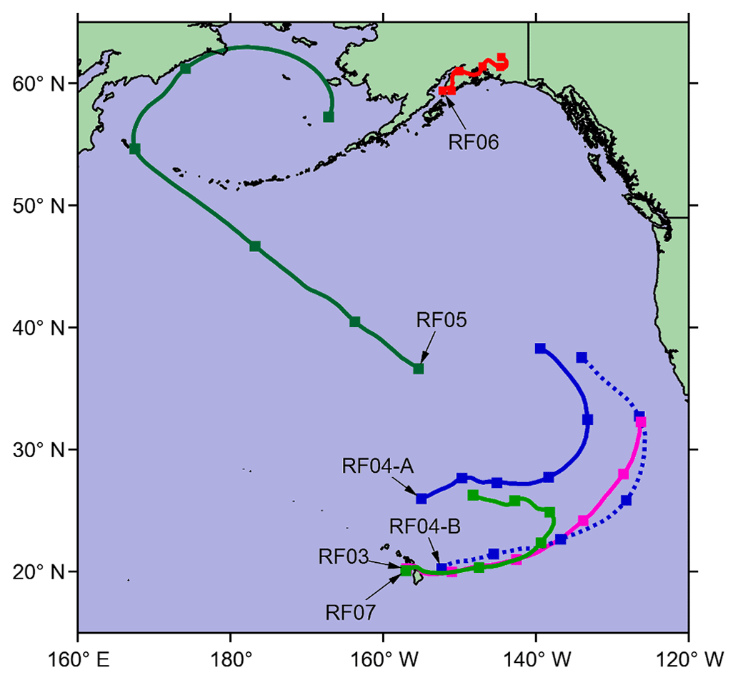
Figure 1 Map of flux legs and back trajectories during TI³GER. Square markers indicate 24 h periods, and the arrows mark the location of the flux legs.

Flux legs were typically 5–10 min long. At airspeeds of ∼ 110 m s⁻¹, flux legs covered 30–70 km. A typical flight module consisted of three legs flown in a stacked manner (RF03-B, RF03-C, and RF07-A). However, in the case of RF03-B, fluxes were below detection. Hence, other flight legs were opportunistically used for flux calculations on level legs in the marine boundary layer (MBL). Dedicated flux segments were accompanied by profile descents and ascents.

2.2 Ozone instrumentation

Three ozone instruments were installed on the GV. Two (the FAIRO instruments) were of an identical design.

2.2.1 The NCAR Fast O₃ instrument

The NCAR Fast O₃ instrument sampled from the HIAPER Modular Inlet (HIMIL). All tubing was made of Teflon. The total mass flow in the inlet was 2370 sccm. The sample line was 70 cm long with an inner diameter of 6.4 mm. From this flow, Fast O₃ sampled 500 sccm through a 140 cm long line with an inner diameter of 3.8 mm at a constant absolute pressure of 70 Torr. Total residence time is 0.75 s. Fast O₃ provides 10 Hz data by detecting photons from the following chemiluminescence reaction:

$$\begin{array}{}\text{(R1)}& {\displaystyle }{\mathrm{O}}_{\mathrm{3}}+\mathrm{NO}\to {\mathrm{O}}_{\mathrm{2}}+{{\mathrm{NO}}_{\mathrm{2}}}^{\ast }\text{(R2)}& {\displaystyle }{{\mathrm{NO}}_{\mathrm{2}}}^{\ast }\to {\mathrm{NO}}_{\mathrm{2}}+h\mathit{\nu }.\end{array}$$

The excited NO₂ in Reaction (R2) can also be quenched by collision with other molecules. Water vapor quenches excited NO₂ more efficiently than do nitrogen or oxygen (Matthews et al., 1977), so after time stamp synchronization among the instruments (see Sect. 2.4), the following water vapor correction is applied (Ridley et al., 1992):

$$\begin{array}{}\text{(1)}& {\left[{\mathrm{O}}_{\mathrm{3}}\right]}_{\mathrm{corrected}}=\left[{\mathrm{O}}_{\mathrm{3}}\right]\times \left(\mathrm{1}+\mathrm{4.3}\left(\pm \mathrm{0.3}\right)\times {\mathrm{10}}^{-\mathrm{3}}\times \left[{\mathrm{H}}_{\mathrm{2}}\mathrm{O}\right]\right),\end{array}$$

where [O₃] is the ozone mixing ratio in ppbv, and [H₂O] is the water vapor mixing ratio in per mill by volume of dry air.

The water vapor correction is performed using vertical-cavity surface-emitting laser (VCSEL) water vapor data (see Sect. 2.3) that are collected at a higher frequency (25 Hz) than the Fast O₃ data are. Thus, the water vapor correction is expected to contribute negligible bias to the EC flux calculations. To assess the potential impact of the water vapor correction on Fast O₃ EC fluxes, the constant in Eq. (1) was varied from its minimum and maximum estimated values (4.0–4.6) in the RF03-C-2 leg; the change in this parameter resulted in biases in the EC flux results of no more than 0.7 %. Neglecting the water vapor correction altogether decreased the calculated exchange velocity (see Sect. 2.5) by 5 % from 0.131 to 0.124 cm s⁻¹ (see Table 2). Using the average water vapor concentration during the entire leg for the water vapor correction increases the calculated exchange velocity 2 % to 0.134 cm s⁻¹; this case represents the extreme case in which water vapor reaching the ozone instruments is completely smeared out by longitudinal diffusion. We conclude that water vapor interference in the Fast O₃ instrument contributes at most 5 % to the ozone flux uncertainty and likely less than 2 %. The 0.131 cm s⁻¹ value is in good agreement with the EC flux results from FAIRO 1 and FAIRO 2, and the Fast O₃ exchange velocities are not systematically higher or lower than those from FAIRO 1 or FAIRO 2. The water vapor interference for the coumarin instruments goes in the opposite direction to that for the UV instruments; i.e., water vapor makes Fast O₃ less sensitive to ozone but FAIRO more sensitive (Güsten et al., 1992; Schurath et al., 1991; Zahn et al., 2012). The fact that all three instruments agree after water vapor correction gives us confidence that water vapor bias is removed. The Fast O₃ instrument was calibrated after the campaign using a TECO Model 49i-PS ozone primary standard. The typical instrument detection limit is 0.5 ppbv Hz^−0.5 with an accuracy not better than 5 % at high signal to noise.

2.2.2 The KIT Fast AIRborne Ozone (FAIRO) instruments

Two identical FAIRO instruments were deployed. The FAIRO instruments were independently checked for proper functioning both prior to the campaign using an Ansyco (now Gasmet Technologies) SYCOS KT-O3M and after the campaign using a TECO-49i-PS. The FAIROs sampled from a separate HIMIL (aft-facing inlet line) through a PFA line with a length of 4.3 m and a 0.42 cm ($\mathrm{1}/\mathrm{6}$ in.) inner diameter. Outside air was pulled at 11 vol.-L min⁻¹ at ambient pressure by a Vacuubrand MD1 pump downstream of the instruments. Residence time in the line is approximately 0.3 s. The flow was split at a T-fitting ∼ 0.5 m ahead of the FAIROs. Internally, 2.5 vol.-L min⁻¹ of flow went to the UV photometer, which measured ozone absorption around 255 nm within the Hartley band. The O₃ absorption cross section and temperature dependence are taken from Barnes and Mauersberger (1987). The UV absorption channel operates at 0.25 Hz. A second, faster 12.5 Hz coumarin chemiluminescence detector (CID) (Ermel et al., 2013) is calibrated against the UV channel and provides the data used in EC flux calculations. The dual-detector FAIRO design has two main advantages over the Fast O₃ instrument: the FAIROs are lightweight (approx. 14 kg, 19 in. rack slot with three height units per instrument) and do not require operating fluids such as compressed gases. Scattering by aerosols and absorption by aromatic compounds and water vapor are well-known interferences for UV ozone instruments (Dunlea et al., 2006). The potential for humidity changes to interfere with FAIRO UV photometers was further investigated and was found to be small yet not fully insignificant (see Fig. S1 in the Supplement). Interference from aerosols is avoided by the backward-facing sample inlet, and aromatic compounds are expected to be minimal in the pristine air sampled in RFs 03–07. A detailed technical description of FAIRO CID can be found in Zahn et al. (2012). The instrument detection limit is below 1 ppbv Hz^−0.5 (provided by the CID) and the total uncertainty 1.5 % (mainly determined by the uncertainty of the O₃ absorption cross section found in the literature) or 1.5 ppbv, whatever is lower.

2.3 Water vapor: VCSEL

Water vapor in the free stream above the GV is measured by the vertical-cavity surface-emitting laser (VCSEL) hygrometer. VCSEL is an open-path optical cavity measuring two absorption lines for a high dynamic range: a strong line at 1854.03 nm for low volume mixing ratios (VMRs) and a weak line at 1853.37 nm for high VMRs. Data are collected at 25 Hz. During the flux legs, water vapor is always above the VCSEL detection limit of 0.8 ppmv. Details about the operation of VCSEL can be found in Zondlo et al. (2010).

2.4 Instrument time stamp synchronization

The three ozone instruments and the GV variables are measured for four independent time stamps, each with its own potential offset and drift. Conveniently, ozone and water vapor VMRs are occasionally anticorrelated (and, less frequently, correlated). We use these anticorrelation events to synchronize each ozone instrument with VCSEL since VCSEL is already synchronized with the anemometer. First, the ozone and VCSEL signals are interpolated to a common 100 Hz time stamp. Second, each ozone time series is visually inspected to identify unambiguous anticorrelation events with the water vapor time series in the periods before and after each flux leg. Third, the time lag of each anticorrelation event is determined by shifting the interpolated ozone signal until the absolute value of the covariance between the ozone and VCSEL signals is maximized. Finally, with the time lag identified both before and after the leg, the ozone time stamp is linearly stretched to match the VCSEL time stamp. Anticorrelation events are not uncommon. For instrument intercomparison, anticorrelation events from the start and end of the entire flight are used to synchronize data; averaging the synchronized data over 10 s is sufficient to resolve any residual (< 100 ms) synchronization uncertainty. For flux sampling, anticorrelation events were found before and after each flux leg.

2.5 Eddy covariance flux calculations

Eddy covariance (EC) is a commonly used technique to determine the fluxes of gases in well-mixed surface layers. Given chemical concentration and wind speed data, EC flux can be calculated as

$$\begin{array}{}\text{(2)}& \text{EC flux}=\text{cov}(x,w)={\displaystyle \frac{\mathrm{1}}{n}}{\sum }_{i=\mathrm{1}}^n\left(x_i-\stackrel{\mathrm{‾}}{x}\right)\left(w_i-\stackrel{\mathrm{‾}}{w}\right),\end{array}$$

where x is the concentration of the chemical species and w is the vertical wind component. For non-stationary conditions, wavelet analysis (WA) is commonly employed instead (Torrence and Compo, 1998). Stationarity is not required for WA because WA decomposes the total flux into component fluxes at different frequencies. In WA, the time series are first transformed into a wavelet by convolution with a wavelet function:

$$\begin{array}{}\text{(3)}& {\displaystyle }{W}_{\mathrm{s}}(a,b)=\underset{-\mathrm{\infty }}{\overset{\mathrm{\infty }}{\int }}s\left(t\right){\mathit{\psi }}_{a,b}\left(t\right)\mathrm{d}t,\text{(4)}& {\displaystyle }{\mathit{\psi }}_{a,b}\left(t\right)={\displaystyle \frac{\mathrm{1}}{\sqrt{a}}}{\mathit{\psi }}_{\mathrm{0}}\left({\displaystyle \frac{t-b}{a}}\right),\end{array}$$

where a and b are scale and translation factors for ψ₀, the prototypical (or “mother”) wavelet function. For eddy covariance applications, the typical choice for the mother wavelet is the Morlet wavelet:

$$\begin{array}{}\text{(5)}& {\mathit{\psi }}_{\mathrm{0}}\left(\mathit{\eta }\right)={\mathit{\pi }}^{\frac{-\mathrm{1}}{\mathrm{4}}}{e}^{i{\mathit{\omega }}_{\mathrm{0}}\mathit{\eta }}{e}^{\frac{-{\mathit{\eta }}^{\mathrm{2}}}{\mathrm{2}}}{\mathit{\omega }}_{\mathrm{0}}=\mathrm{6}.\end{array}$$

The WA flux is then calculated as |W_wW_x|, where W_w and W_x are the wavelet coefficients of wind and ozone, respectively (Wolfe et al., 2018).

A challenge in EC flux error analysis is that EC flux is not a measurement from a single instrument but rather the combination of measurements from two instruments: a chemical monitor of some sort and an anemometer. For individual instruments, estimation of the limit of detection (LOD) from random error (RE) can be straightforward:

$$\begin{array}{}\text{(6)}& \text{LOD}=\mathit{\alpha }\times \text{RE},\end{array}$$

where α is a dimensionless factor corresponding to the confidence level (1.96 for 95 % CL, 3 for 99 % CL). The standard deviation of blank measurements can be used to estimate the RE of a single instrument. However, this method is not applicable to flux measurements due to the lack of true “blanks” matching the chemical and meteorological conditions of interest.

Several methods for determining the LOD of EC flux measurements have been put forth based on statistical treatments of the cross-covariance of the chemical and wind data at different time lags. For example, Langford et al. (2015) present the following formula for estimating the root mean squared error (RE_RMSE):

$$\begin{array}{}\text{(7)}& \begin{array}{rl}& {\mathrm{\text{RE}}}_{\mathrm{RMSE}}\\ & =\sqrt{\mathrm{0.5}\left({\left({\mathit{\sigma }}_{f_{w^{\prime }{c^{\prime }}_{\left[-\mathrm{\Gamma }\right]}}}\right)}^{\mathrm{2}}+{\left({\stackrel{\mathrm{‾}}{f}}_{w^{\prime }{c^{\prime }}_{\left[-\mathrm{\Gamma }\right]}}\right)}^{\mathrm{2}}+{\left({\mathit{\sigma }}_{f_{w^{\prime }{c^{\prime }}_{\left[+\mathrm{\Gamma }\right]}}}\right)}^{\mathrm{2}}+{\left({\stackrel{\mathrm{‾}}{f}}_{w^{\prime }{c^{\prime }}_{\left[+\mathrm{\Gamma }\right]}}\right)}^{\mathrm{2}}\right)},\end{array}\end{array}$$

where ${\mathit{\sigma }}_{f_{w^{\prime }{c}^{\prime }}}$ and $\stackrel{\mathrm{‾}}{f_{w^{\prime }{c}^{\prime }}}$ are the standard deviation and average of the cross-covariance, and ±Γ represents time lags far away from the true time lag between the wind and chemical measurements. Currently, no well-established method for estimating the LOD of EC and WA fluxes is commonly accepted. The number of independent replicate measurements of ozone available during TI³GER gave us the unique opportunity to explore, evaluate, and optimize methods to constrain the uncertainty of EC fluxes, since the standard deviation of the fluxes measured between the individual instruments can give a sense of the magnitude of the “true” error.

A MATLAB toolkit (Wolfe, 2023) was used for this work. Raw data must be pre-processed to remove data gaps before inputting to the toolkit. Data gaps are removed by linear interpolation; such gaps are rare, and interpolation is used only to remove up to three or four points (out of ∼ 2000–4000, which is typical of a flux leg). Because the GV data are recorded at higher resolution than the ozone data are, the wind and VCSEL data are binned to each ozone instrument's corrected time stamp.

For EC fluxes, the toolbox detrends the data with a boxcar method in a user-defined time frame. The lengths of the detrending time frames were selected to balance being short enough to remove systematic cross-covariance structures with being long enough to retain low-frequency fluxes. A detrending time of 10 s was used in all fluxes presented below. For all flux legs, various detrending times were tested to see whether visually identifiable structures could be observed in the cross-covariance. A uniform 10 s detrending time was found to remove systematic structures from all flux legs. To minimize the number of subjective inputs, we did not attempt to customize the detrending time for each flux leg. Because detrending accounts for meteorological conditions rather than instrument response, meaningful intercomparisons could be performed using uniform conditions and consistent detrending times. At typical aircraft speeds, 10 s corresponds to 1–1.2 km. In addition to calculating an eddy covariance flux, the toolbox also calculates WA flux (Torrence and Compo, 1998) and output cospectra as a function of frequency.

In contrast to common practice, we express ozone fluxes in terms of exchange velocity (v_e) rather than deposition velocity (v_d), where

$$\begin{array}{}\text{(8)}& v_{\mathrm{e}}={\displaystyle \frac{\text{flux}\left(\mathrm{ppb}\mathrm{m}{\mathrm{s}}^{-\mathrm{1}}\right)}{\text{concentration}\left(\mathrm{ppb}\right)}}\times {\displaystyle \frac{\mathrm{100}\mathrm{cm}}{\mathrm{1}\mathrm{m}}}.\end{array}$$

Exchange velocity is the same as deposition velocity apart from the lack of a negative sign; i.e., upward-directed fluxes have positive v_e. We use v_e rather than v_d because some interesting case studies presented have upward-directed fluxes, which are more intuitively represented using positive signs.

Notably, fluxes and cross-covariances in principle have the same units (molec. cm⁻² s⁻¹ or ppb m s⁻¹). However, we use “covariance” to refer to the cross-covariance calculated for different lag times by our code and “flux” to identify an atmospheric state. This distinction is useful when discussing EC flux errors, which are estimated from cross-covariances at time lags departing from the true lag between instruments. Whereas such cross-covariances represent true statistical covariance, they do not represent atmospheric fluxes.

3 Results and discussion

3.1 Instrument intercomparison

Figure 2 shows the time series of O₃ from all three sensors from RF03 as an example. Panel (a) shows the altitude of the GV, and panel (b) shows the water vapor and ozone time series for the entire flight. Water vapor–ozone time synchronization was performed as close to the beginning and the end of the flight as correlation events could be visually identified; close-ups of these events are shown in panels (c) and (e). For EC flux legs, time synchronization was performed before and after each leg rather than for the entire flight. Because the Fast O₃ instrument computer was not synchronized with the time server, there was an artificial delay of 5 s between it and VCSEL. After the time synchronization procedure, even artificial clock delays are resolved to within ± 0.1 s. However, panel (d) shows that the ozone signals are not synchronized with each other or to a water vapor correlation event midway through the flight. The discrepancy could be caused by a combination of different flow conditions at different altitudes or instrumental clock drift. However, because the FAIRO instruments share an inlet line that forks only in the last ∼ 0.5 m, inlet line flow differences alone cannot explain their time offset. Inspection of the delays from each RF shows that the ozone clocks drift no more than ± 0.7 s (typically ≤ 0.5 s). For ozone instrument comparisons, data were averaged over 10 s to prevent bias from synchronization errors.

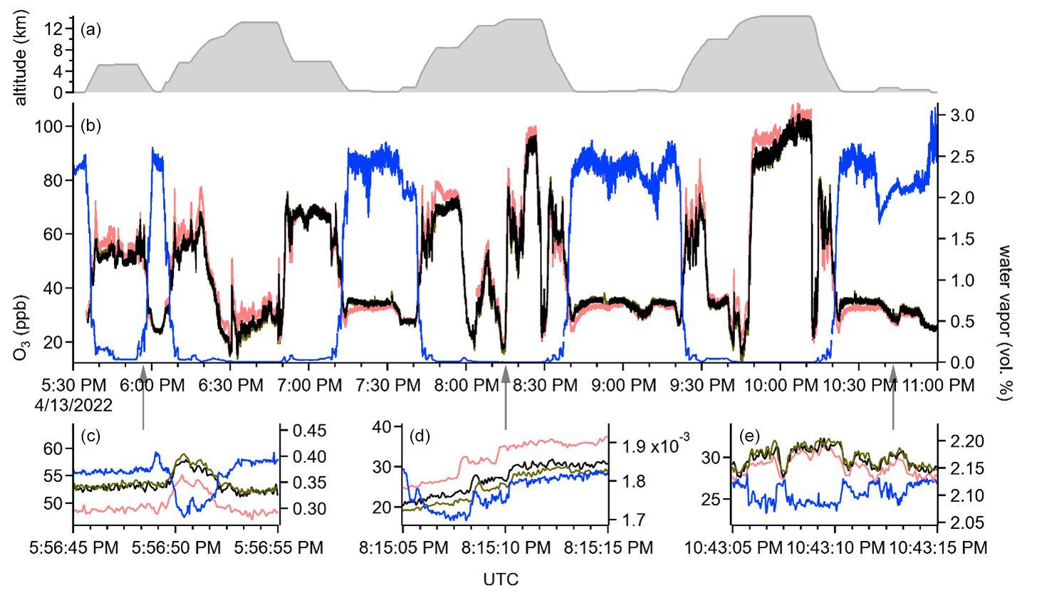
Figure 2 Time stamp synchronization based on the H₂O and O₃ time series. VCSEL data are shown in blue, Fast O₃ data in salmon, FAIRO 1 in black, and FAIRO 2 in dark olive. All traces are shown at the native instrument resolution (25 Hz for VCSEL, 12.5 Hz for the FAIROs, and 10 Hz for Fast O₃). (a) Altitude time series. (b) Time series for the entire flight. (c–e) Zoomed-in views of cross-covariance events, with gray arrows pointing to exact times.

Aggregated data from RF03—07 are shown in Fig. 3a. Ozone VMRs measured by each FAIRO are plotted against ozone VMRs measured by Fast O₃. Linear fits of the FAIRO VMRs are also shown. The data from both instrument designs appear to be linear, with a 2 % overall difference. In panels (b)–(d), the absolute and relative differences between each instrument and the average of all three instruments are shown. In all cases, data are color-coded for high water vapor (concentration > 1.4 × 10¹⁷ molec. cm⁻³, blue) and high NO_x (volume mixing ratio > 200 pptv, red). GPS altitude, VCSEL water vapor concentration, and NO_x are also shown in the background of panels (b), (c), and (d), respectively, for context. Neither the absolute nor the relative differences from the average exhibit systematic behavior depending on water vapor or NO_x. The effect of humidity changes did not reveal any obvious explanation for O₃ differences when comparing individual instruments to the instrument mean (not shown). For the effect of changing humidity when comparing FAIRO instruments, see Fig. S1; for the effect of changing humidity on FAIRO to Fast O₃ comparison, see Fig. S2. Although the persistent differences from average are accompanied by high-NO_x conditions between ∼ 00:00 and 02:00 UTC on 21 April 2022, high-NO_x conditions between ∼ 19:30 and 20:00 UTC on 20 April 2022 are not accompanied by similar differences. High water vapor during a low-altitude flux leg at 21:00 UTC is accompanied by agreement amongst all three instruments within 2 %.

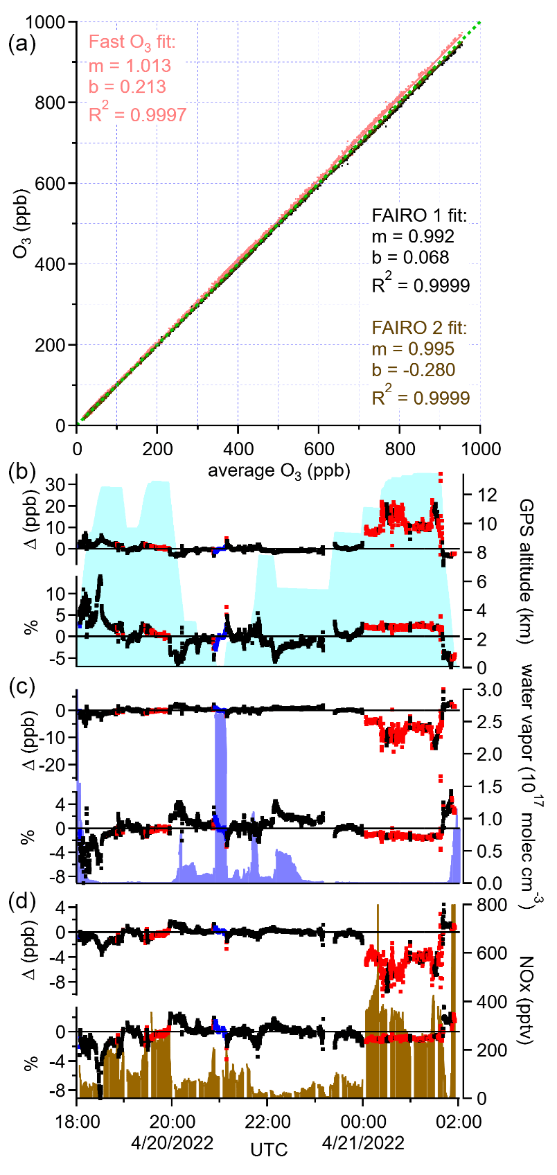
Figure 3 (a) Aggregated data from RF03–07 with fits relative to global average, with the 1 : 1 line in green. Absolute and relative differences from average during RF05 for Fast O₃ in panel (b), FAIRO 1 in panel (c), and FAIRO 2 in panel (d). Background shading for GPS altitude in panel (b), VCSEL in panel (c), and NO_x in panel (d).

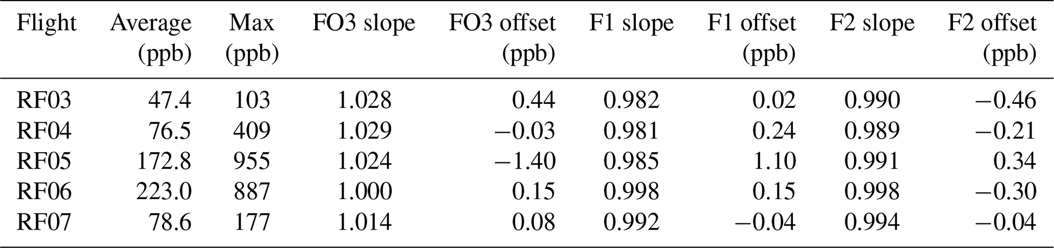
The agreement of the instruments was also evaluated individually for RFs 03–07. The fit results for each flight are shown in Table 1.

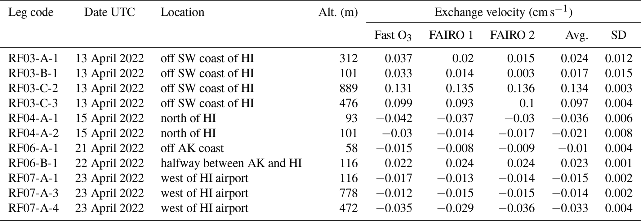
Table 1 Linear fit parameters of individual instruments to average. F1 and F2 refer to FAIROs 1 and 2, respectively.​​​​​​​

A subset of flux legs with low ozone variability was used to infer an upper limit of the precision of each instrument, as the contribution by additional atmospheric variability cannot be fully eliminated. The ozone time series from each flux leg is smoothed over 1 s, and the range of the smoothed data is calculated. Variability is calculated as the relative range of ozone in that leg. Flux legs are characterized as having low variability if the relative range of the smoothed time series is less than 5 % for at least two instruments. Precision is calculated as the standard deviation of the unsmoothed time series. All three instruments have comparable precision, with Fast O₃ precision at 1.4 % (0.45 ppb) at 10 Hz, FAIRO 1 at 1.2 % (0.36 ppb) at 12.5 Hz, and FAIRO 2 at 1.1 % (0.36 ppb) at 12.5 Hz. These precision estimates represent an upper bound as some of the variability could be true atmospheric variability. More detail on the precision calculations can be found in Table S2.

3.2 Eddy covariance flux

Potential temperature (Θ) and equivalent potential temperature (Θ_e) profiles are used to determine whether flux legs were conducted within the MBL. Example profiles are shown in Fig. 4. The profiles shown are taken from both descent and ascent except in the case of the RF03-C flux legs, which were performed as the plane approached the airport for landing. The flux legs in RF04 were conducted over the tropical Pacific Ocean, and both profiles indicate an MBL height of ∼ 800 m. The utility of Θ_e in determining the MBL height is evident in the RF06-A legs, which were conducted off the coast of Alaska. The Θ profile on the descent does not unambiguously show an MBL height, but the Θ_e profile clearly indicates an MBL height of ∼ 200 m on both the descent and ascent. Such a shallow MBL near the Kenai Fjords combined with the strong temperature inversion suggests RF06-A may be subject to distinct “pools” of air; yet the Θ_e profiles suggest mixing up to the surface. The MBL height in RF03-A is difficult to distinguish and may be ∼ 500 m. In all cases, flux legs were conducted at heights well within the MBL except in RF03, where flux legs were conducted at 107, 476, and 889 m.

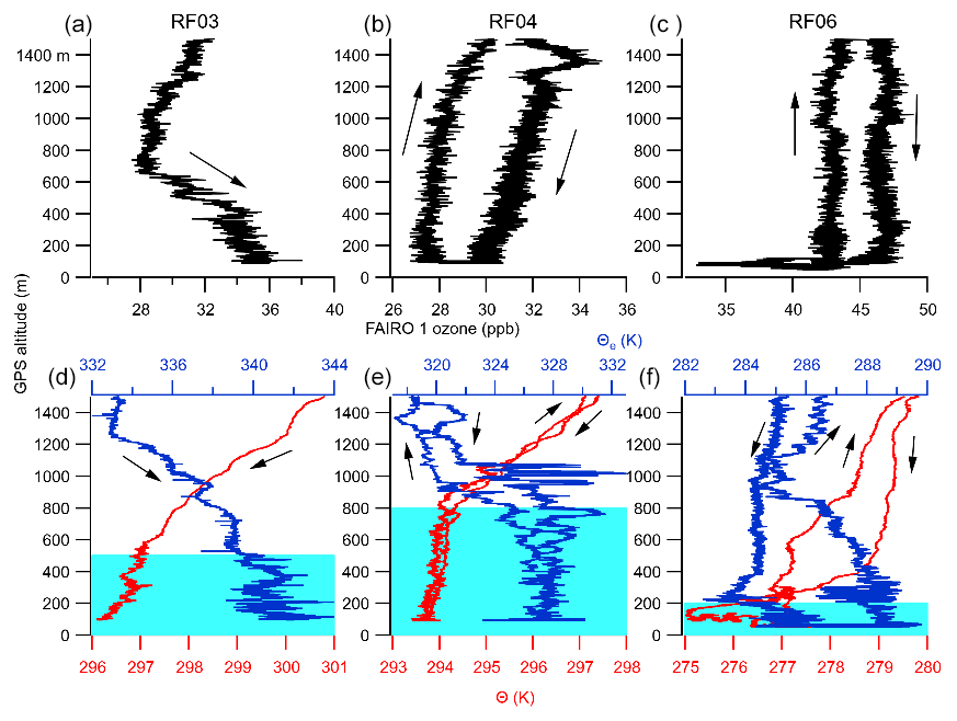
Figure 4 (a–c) Profiles of ozone during RF03-C, RF04-A, and RF06-A, respectively. (d–f) Corresponding potential temperature and equivalent potential temperature profiles for RF03-C, RF04-A, and RF06-A, respectively. MBL height is shown as light-blue shading. Arrows indicate profile ascents and descents.

Whereas the Fast O₃ instrument used constant mass flow at constant pressure, the FAIRO instruments used constant volume flow at ambient pressure. In principle, the flow rates in the two instrument designs could differ between the high-altitude–low-pressure legs typically used for time synchronization and the low-altitude–high-pressure legs used for flux measurements. Although the different flow rates can create a time lag between wind and ozone data, no systematic error is introduced into the ozone flux because we empirically determine the time offset and do not prescribe a constant offset in the MATLAB flux toolkit. Rather, the time synchronization is used in conjunction with water vapor fluxes calculated from VCSEL data to find the true ozone time offset.

The time delay between VCSEL and the wind data is determined by calculating the water vapor flux. VCSEL and wind speed data are well synchronized; in most (12) cases, the water vapor cross-covariance had a peak at a time lag of zero points, and in six cases, the optimal lag was −1 point on the 12.5 Hz FAIRO time stamp (within 0.08 s). In one case (RF07-A-4) the VCSEL cross-covariance peaked at +5 points, but this is likely a spurious correlation because the VCSEL data from the previous leg were well synchronized (zero time lag). Cross-covariance and cospectra for ozone and water vapor are shown for selected flux legs (RF03-C-2, RF04-A-1, and RF06-A-1) in Fig. 5 (see Sect. 3.4).

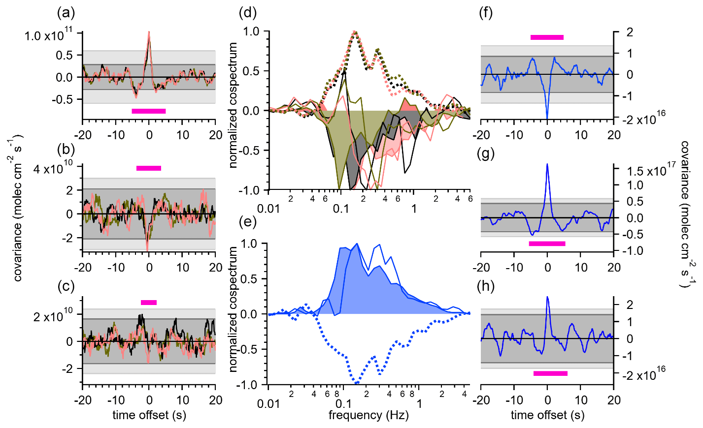
Figure 5 Cross-covariance plots for RF03-C-2 (a), RF04-A-1 (b), and RF06-A-1 (c) and their respective water vapor fluxes (f–h). Normalized cospectra are shown in panels (d) and (e). Detrending the data at 10 s removes spectral power and frequencies below 0.1 Hz. For ozone data, Fast O₃ is shown in salmon, FAIRO 1 in black, and FAIRO 2 in olive. In panels (d) and (e), RF03 is shown as a dotted line, RF04 as a shaded line, and RF06 as a solid line. Integral timescales are shown as fuchsia bars.

Because water vapor fluxes are strong and always above detection, the VCSEL-to-wind time offset allows us to anchor the ozone time offset and limit our search for an ozone covariance peak to ±0.7 s from the VCSEL time offset since that is the maximum observed ozone-to-VCSEL time delay. An ozone flux is only reported for an instrument if a cross-covariance peak is found within that window. A flux is not reported for an instrument if the covariance behavior within that window is primarily one of sign change, e.g., if the covariance linearly increases from negative to positive or if there are many zero crossings. If all three instruments show a covariance that survives this filter, then an average flux is reported for that leg. Of the 19 flux legs, 11 had fluxes that met this criterion, and they are summarized in Table 2. A full version of Table 2 with meteorological conditions and other compounds of interest is included in the Supplement. The cospectra in Fig. 5 peak from 0.1–0.2 Hz, indicating that the bulk of the fluxes occur at 5–10 s timescales. These timescales are typical of fluxes in the MBL and an order of magnitude larger than the mixing time for the Fast O₃ instrument, which for background characterization purposes had zero air injected from the aircraft inlet. The e-fold rise time was < 0.5 s, fast enough not to introduce bias into the flux measurements (see Fig. S3). Indeed, the cumulative frequency graph (ogive) shows that in the case of RF03-C-2, less than 10 % of the total flux is carried on < 1 s timescales. Ogives are shown in Fig. S4. The residence time in the fast ozone instrument detection volume implied a maximum frequency response of 9 Hz. However, high pass attenuation in the inlet manifold limited the frequency response of the Fast O₃ instrument to 3 Hz (Lenschow and Raupach, 1991). The FAIRO instruments were not equipped with zero-air injection at the inlet. However, the residence time in the FAIRO flow is shorter than that in Fast O₃. A calculation of the FAIRO inlet manifold indicates attenuation of high-frequency signals above 20 Hz, and therefore this was not the limiting factor in the FAIRO instrument frequency response. Thus, the FAIRO was more sensitive to high-frequency fluxes than the Fast O₃ instrument.

Table 2 ​​​​​​​Summary of ozone EC flux results.

3.3 Comparison with literature

A previous study has compared ozone EC flux measurements from dry chemiluminescence ozone instruments over grassland (Muller et al., 2010), but to our knowledge no instrument intercomparisons have been performed on board aircraft. Aircraft measurements of ozone flux have been reported before over land (Lenschow et al., 1980; Wolfe et al., 2015, 2018) and over the ocean during PASE (Conley et al., 2011). In the latter, ozone exchange velocities were −0.024 ± 0.014 cm s⁻¹. Larger datasets for marine ozone flux have been produced by ship campaigns. The TexAQS cruise reported ozone exchange velocities as large as −0.81 ± 0.27 cm s⁻¹ in coastal channels and −0.034 ± 0.003 cm s⁻¹ in offshore areas, and the STRATUS cruise measured −0.009 ± 0.001 cm s⁻¹ over open-ocean areas (Bariteau et al., 2010; Helmig et al., 2006). All three instruments tested here can detect exchange velocities in the lower range observed in the remote ocean.

3.4 Constraining the error estimate

Figure 5 shows three examples of covariance plots from flux legs that are representative of the range of conditions observed. Ozone plots are shown on the left, and the corresponding plots for VCSEL are shown on the right. For all cross-covariances, the Langford LOD is calculated using Γ = 30 s at the beginning and end of the cross-covariance plot, and the Langford 99 % CL LOD for Fast O₃ is shown with light-gray shading. Panel (a) (RF03-C-2) is a case in which all three ozone instruments measured an upward-directed flux, and VCSEL (panel f) shows water vapor directed downward toward the ocean; this case is described in more detail below. Panel (b) (RF04-A-1) shows ozone depositing into the ocean and water vapor evaporating out of the ocean. These two cases are examples of EC flux strong enough to be unambiguously identified by all three ozone instruments; i.e., each instrument's flux measurement is above the LOD as defined by Langford et al. (2015).

Panel (c) (RF06-A-1) shows a case in which no ozone-instrument-derived flux is above the Langford LOD. Viewed in isolation, no instrument's cross-covariance is convincing on its own. However, a small candidate peak can be identified within the ±0.5 s interval.

The average exchange velocity measured by all three instruments in RF06-A-1 is −0.010 cm s⁻¹ with a standard deviation of 0.004 cm s⁻¹. The Langford RE_RMSE for this leg corresponds to 0.0057–0.0074 cm s⁻¹ depending on the instrument and thus overstates the error and LOD. We propose a modification of the Langford approach by restricting the interval Γ by calculating the integral timescale. The integral timescale τ characterizes the period over which covariance persists. We estimate τ by integrating outward from the peak until the integral crosses zero (Lenschow et al., 2000). It is possible in certain cases for the calculation of τ to fail. This happened for the VCSEL data shown in panel (h) (RF06-A-1). In this case τ was estimated as the width between the second zero crossings from the peak.

We then apply the Langford RE_RMSE calculation to intervals +Γ and −Γ, which are τ in length and are centered around relatively smooth areas of cross-correlation near the candidate peak. Identifying “smooth” areas was necessarily subjective as the cross-correlation behavior is unique to each leg. The 99 % LOD calculated in this modified approach is shown in Fig. 5 as dark-gray shading. The RE_RMSE estimated by the modified approach corresponds to 0.0053–0.0064 cm s⁻¹, which is more in line with the “true” random error among the three measurements.

3.5 Spatial variability of ozone and water vapor fluxes

The fluxes of ozone and water vapor were in the counterintuitive directions during the RF03-C legs. Figure 6 shows profiles, fluxes, and flight movie stills from this leg. Water vapor was carried downwards, although the ocean surface is usually a water vapor source by evaporation. Conversely, ozone was carried upwards, even though the ocean surface is expected to be an ozone sink. The ozone exchange velocity in this leg (RF03-C-2) was +0.134 cm s⁻¹ measured at an altitude of 889 m. At a lower altitude of 476 m (RF03-C-3), the exchange velocity was +0.097 cm s⁻¹. These velocities are consistent with the lower range of nocturnal entrainment velocities (0.12–0.72 cm s⁻¹) measured during the DYCOMS-II campaign over the eastern Pacific Ocean (Faloona et al., 2005).

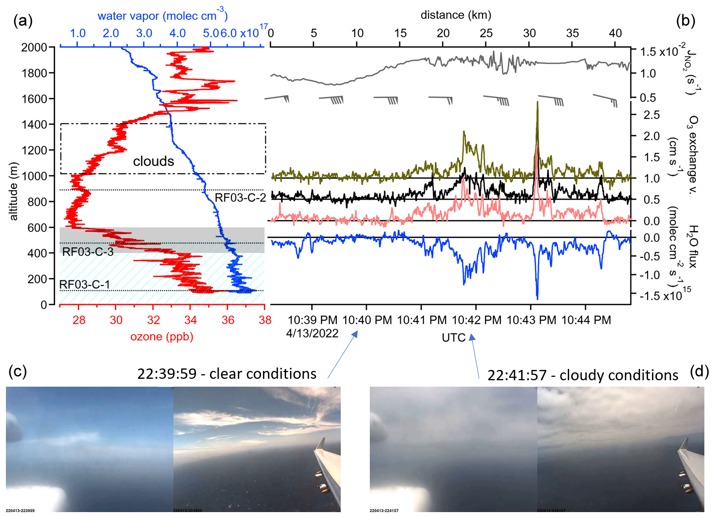
Figure 6 (a) Ozone and water vapor vertical profiles and time series for EC fluxes from the RF03-C leg. Ozone profile is the average of all three instruments. Dashed lines indicate flight altitudes, and the dashed rectangle represents visually estimated cloud layer. (b) $J_{{\mathrm{NO}}_{\mathrm{2}}}$ (gray) and fluxes from Fast O₃ (salmon), FAIRO 1 (black), FAIRO 2 (olive), and VCSEL (blue). Vertical offsets of 0.5 and 1 cm s⁻¹ have been added to FAIRO 1 and 2 to better illustrate the close agreement between the three O₃ instruments. (c, d) Images of the webcams from RF03 flight movies illustrate cloud cover conditions.

The entrainment velocity as defined by Deardorff (1976) is modified here, as in exchange velocity, such that the upward flux is positive:

$$\begin{array}{}\text{(9)}& w_{\mathrm{e}}={\displaystyle \frac{\text{flux}\left(\mathrm{ppb}\mathrm{m}{\mathrm{s}}^{-\mathrm{1}}\right)}{\mathrm{\Delta }-\text{concentration}\left(\mathrm{ppb}\right)}}\times {\displaystyle \frac{\mathrm{100}\mathrm{cm}}{\mathrm{1}\mathrm{m}}}.\end{array}$$

In Eq. (9), Δ concentration is the difference in the concentration of a species across a boundary to the mixed layer. In previous work, the flux in the transition layer (TL) was extrapolated from the measured fluxes in stacked legs within the MBL and used to estimate the entrainment velocity (Faloona et al., 2005; Wolfe et al., 2015). This method is not applicable to the RF03-C legs because the conditions are not mixed to the surface and because RF03-C-2 is flown en route to the airport in a decoupled TL characterized by minimum O₃ concentrations and a partial cloud layer near the top (visually estimated from flight videos as ∼ 1 km). The MBL below extends to ∼ 500 m, and the entrainment velocity measured during RF03-C-3 at this altitude (Fig. 6a, shaded) is 6.3 times smaller than the exchange velocity based on the observed ΔO₃ of 5.2 ppb and Eq. (9) (existence of a concentration change is not necessarily indicative of a flux). Contributions due to entrainment of ozone from the free troposphere would result in a negative exchange velocity during RF03-C-2 (the O₃ profile increases with altitude in the free troposphere) and cannot explain the positive O₃ exchange velocity observed. If there were a significant O₃ entrainment from aloft, the observed positive O₃ exchange velocity would have a lower limit.

Furthermore, the temporal correlation between the O₃ and H₂O fluxes along RF03-C-2 is consistent with neither entrainment from above nor detrainment from below as a driver of the observed exchange velocities, since the H₂O profile is continuously decreasing with altitude. The negative H₂O flux during RF03-C-2 cannot be explained by entrainment from above or from below. Overhead cloud cover can be qualitatively estimated from NO₂ photolysis frequency ($J_{{\mathrm{NO}}_{\mathrm{2}}}$) measured by the HIAPER Airborne Radiation Package (HARP) actinic flux instrument (Fig. 6b). During cloud-free portions of RF03-C-2 the exchange velocity approaches zero for both H₂O and O₃, indicating that the observed exchange velocities are cloud related. There are only two possible explanations: (1) the cloud induces dynamical change to increase O₃ entrainment from the MBL into the decoupled TL (in which case the H₂O source above the aircraft is a lower limit), or (2) the cloud above is a sink of O₃ and a source of H₂O (evaporating cloud). Notably, the WA time series in Fig. 6 reveals a pronounced maximum O₃ exchange velocity of +1.8 cm s⁻¹ at the edge of a cloud. Such a large O₃ exchange velocity would require a 5-fold-larger value of ΔO₃ towards the MBL than is compatible with the observed O₃ profile and would require O₃ concentrations in the MBL well in excess of 50 ppbv. No such elevated O₃ concentrations were observed anywhere near this case study or during landing (the O₃ concentration 2 min before landing was 32 ppbv, compatible with the profile shown in Fig. 6). Detrainment of O₃ from below and entrainment of O₃ from the free troposphere hence cannot explain the observed positive O₃ exchange velocity during portions of RF03-C-2. We conclude that a chemical O₃ sink related to an evaporating cloud is responsible for the lower O₃ (by at least 5.2 ppb) in the decoupled TL.

Previously, it was proposed that an increase in aqueous-phase chemistry in cloud droplets would decrease ozone production in high-NO_x environments and enhance ozone destruction in low-NO_x environments (Lelieveld and Crutzen, 1990). Computational simulations suggest that ozone could be stabilized within the air–water interface (within the first 4 Å) and that modification of the ozone UV–vis absorption cross section and activation of photolytic pathways at the interface can increase the ozone photolysis rate constant by more than a factor of 20 (Anglada et al., 2014). The observations from the RF03-C legs may represent the first field evidence of these proposed processes. Critically, the RF03-C-1 flux leg performed at 107 m immediately prior to the RF03-C-2 887 m leg found fluxes below detection for all three ozone instruments. Thus, if cloud effects are operative, they may well be invisible to surface-based platforms such as ships.

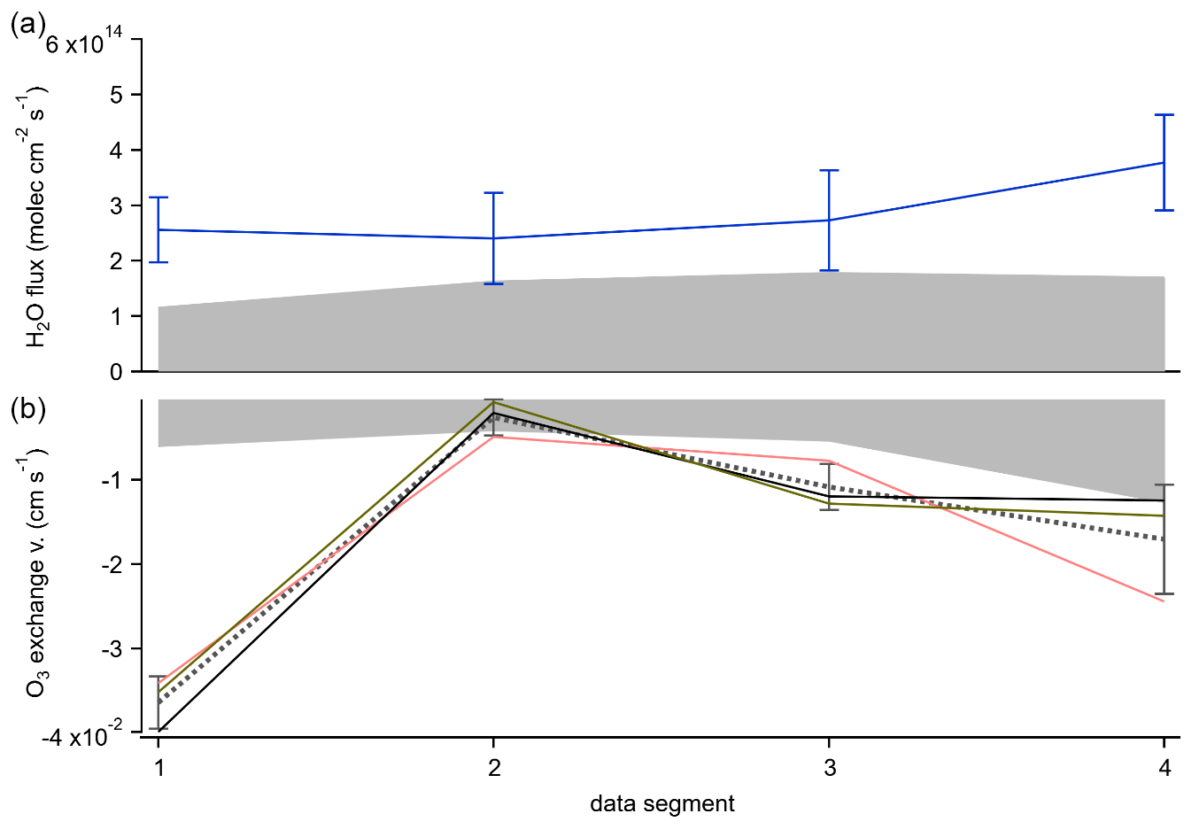
Figure 7 Segments of RF06-A-1. (a) VCSEL is shown in blue. Error bars represent modified Langford RE_RMSE. (b) FO3 in salmon, FAIRO 1 in black, and FAIRO 2 in dark olive. The average is shown as the dotted line. Error bars represent standard deviation. In both panels, the 95 % LOD is shaded. Each data segment is 75 s long.

Compared to shipborne measurements taken over the course of days or weeks, the flux legs here are necessarily shorter, with the longest leg being 10 min and the legs being only ∼ 5 min long on average. To assess the consistency between sensors on shorter timescales, the ozone EC fluxes were also calculated in 75 s long quarters for the flux example RF06-A-1 shown in Fig. 7. The ozone flux observed in this leg is carried in the first, third, and last quarters, with flux in the second quarter below detection. However, the water vapor flux is above detection in all segments and exhibits different trends from the ozone flux. Since the water vapor and ozone are both carried by the same eddies, the difference in behavior cannot be attributed to meteorology. Rather, the ozone flux variability must reflect true heterogeneity in the ocean and/or atmospheric chemical states. NO_x data were unavailable during the first of the four segments. However, during the last three segments, NO_x concentrations are constant, with NO at 10 ± 5 pptv and NO₂ at 30 ± 15 pptv (note the accuracy of the NO₂ sensor is not better than 50 pptv). Unlike the previous case studies presented, RF06-A-1 was flown near the coast of Alaska, where conditions are expected to be different from those over the open ocean. Low NO_x variability rules out apparent ozone flux by titration by emissions from urban or shipping sources.

Assuming chemical measurements are available on similar timescales, the ozone flux can help characterize atmospheric chemistry on ∼ 10 km spatial scales. For measuring average fluxes, we recommend flying multiple flux legs over regions of interest for better statistics as ozone fluxes are often near the LOD.

4 Conclusions and outlook

In the aggregate, Fast O₃ and FAIRO instruments operate at comparable frequencies (10 vs. 12.5 Hz data rate; 3 Hz practical resolution estimated from the mixing time of zero-air puffs at the Fast O₃ inlet), are accurate within 2 %, and have similar LOD at their typical sampling rates (1.5 ppbv). Large excursions in measured ozone VMRs (of up to 30 %, or 5 ppbv difference) are sometimes observed in the ratio of high data rate between the instruments, but the excursions show no systematic behavior with respect to ozone concentration, water vapor, or NO_x. These differences did not occur during the flux legs. From an operational standpoint, the FAIRO design is advantageous because the instrument and pump fit into a single 19 in. rack and require no hazardous NO gas.

Simultaneous, high-frequency H₂O measurements in the free stream are essential for synchronizing the O₃ sensors and wind measurements and provide context to the interpretation of O₃ EC fluxes. Inlet line delays, clock drifts, and small inaccuracies in clock synchronizations lead to time offsets that are difficult to characterize with certainty. Correlation events between water vapor and ozone present direct means for clock synchronization. In principle, an ozone time lag could be prescribed by matching the ozone time stamp to the water vapor time stamp and searching for the time lag at which water vapor flux peaks since the water vapor flux is always above detection. In practice, clock drifts still necessitate a search for a cross-covariance peak in the ozone flux, albeit in a constrained time window.

The availability of three ozone instruments during TI³GER allowed for the estimation of the “true” LOD of the ozone flux (LOD_ECflux) using the standard deviation of the EC fluxes measured by each instrument. We use this information to provide a modified procedure to estimate the error and LOD_ECflux: the RE_RMSE formula (Eq. 7) (Langford et al., 2015) is combined with the concept of “integral timescale” (Lenschow et al., 2000). We find that the “true” LOD_ECflux (defined as the 95 % CI on the mean EC flux) is overestimated by the EC flux uncertainty on an individual sensor when Γ is a large time window (30 s, as used in Lenschow et al., 2000). Estimating the RE_RMSE over a smaller time window shrinks the RE_RMSE and brings the EC flux uncertainty closer to the “true” error inferred from the EC flux standard deviation of three separate sensors, without underestimating the EC flux error. We find that the integral timescale Γ suitable to estimate error is usually a few seconds and define it here as Γ found by integrating outward from a candidate covariance peak until the first zero crossing of the covariance integral. Typical LODs for O₃ exchange velocities are 30 %–50 % lower with shorter Γ, with typical LOD ∼ 0.005 cm s⁻¹, limited by spurious covariance peaks that are clearly non-physical as they exceed the believable bounds of instrument synchronization.

Ozone EC fluxes measured from aircraft in the remote MBL can exhibit significant time variability on the order of minutes (6–10 km). A similar variability is not seen in the H₂O EC fluxes. While the H₂O EC fluxes are spatially more homogeneous and de facto constant (within 25 %), a variability in the O₃ EC fluxes of larger than 600 % is observed and highly significant (above 6σ to below detection) on spatial scales of 20 km. This variability is seen consistently by all three sensors over the open-ocean environments probed here. Cloud cover can reverse the direction of the O₃ and H₂O fluxes, indicating a source of water vapor and a sink for O₃ above the aircraft, consistent with webcam images of clouds. The drivers of the horizontal variability in O₃ EC fluxes directed into the ocean on fine spatial scales are currently not well understood but could relate to changes in overhead cloud cover, as well as possibly variability in ocean and atmospheric states. Future studies are needed and would benefit from repeat legs and measurements of ocean state variables.