Evaluation of Aeolus feature mask and particle extinction coefficient profile products using CALIPSO data

The Atmospheric LAser Doppler INstrument (ALADIN) on board Aeolus was the first high-spectral-resolution lidar (HSRL) in space. It was launched in 2018 and re-entered in 2023. The FeatureMask (A-FM) and extinction profile algorithms (A-PRO) developed for the Earth Cloud Aerosol and Radiation Explorer (EarthCARE) HSRL ATmospheric LIDar (ATLID) have been adapted to Aeolus and called AEL-FM and AEL-PRO, respectively. These algorithms have been purposely built to process low signal-to-noise ratio space-based lidar signals. A short description of the AEL-FM and AEL-PRO algorithms is provided in this paper. AEL-FM and AEL-PRO prototype products (v1.7) have been evaluated using the collocated Cloud–Aerosol Lidar and Infrared Pathfinder Satellite Observations (CALIPSO) vertical feature mask (VFM) product and level 2 aerosol profile product for 2 months of data in October 2018 and May 2019. Aeolus and CALIPSO are both polar-orbiting satellites, but they have different overpass times. The evaluations are focused on desert dust aerosols over Africa. These types of scenes are often stable in space (tens of kilometres) and time (on the order of 0.5–1 h), and thus, a useful number of collocated cases can be collected.

We have found that the AEL-FM feature mask and the CALIPSO VFM show similar aerosol patterns in the collocated orbits, but AEL-FM does not separate aerosol and cloud features. Aeolus and CALIPSO have a good agreement for the extinction coefficients for the dust aerosols, especially for the cloud-free scenes. The Aeolus aerosol optical thickness (AOT) is larger than the CALIPSO AOT, mainly due to cloud contamination. Because of the missing a cross-polar channel, it is difficult to distinguish aerosols and thin ice clouds using the Aeolus extinction coefficients alone.

The AEL-FM and AEL-PRO algorithms have been implemented in the Aeolus level 2A (L2A) processor. The findings here are applicable to the AEL-FM and AEL-PRO products in L2A Baseline 17. This is the first time that the AEL-FM and AEL-PRO products have been evaluated using CALIPSO data.

1 Introduction

The Atmospheric LAser Doppler INstrument (ALADIN) on board the Aeolus satellite from the European Space Agency (ESA) was launched in August 2018 and performed measurements for about 5 years. ALADIN is a high-spectral-resolution lidar (HSRL) designed to measure wind using Rayleigh and Mie channels at the wavelength of 354.8 nm (Stoffelen et al., 2005; Reitebuch et al., 2018). Aeolus measured global wind profiles from the ground surface up to about 25 km. The wind products were assimilated in the ECMWF (European Centre for Medium-Range Weather Forecasts) model and proved to be beneficial for the numerical weather prediction model (Rennie et al., 2020).

Aerosols and clouds can also be measured by Aeolus; however, the lidar is not optimized for aerosol and cloud sensing. For example, both range bins are large (ranging from about 0.25 to 2 km), and the horizontal resolution is also coarse (3–15 km). Despite the limitations of Aeolus with respect to cloud and aerosol remote sensing, valuable information can be extracted, and several algorithms have been developed for the Aeolus level 2A (L2A) aerosol products. The standard correct algorithm (SCA) and Mie correct algorithm (MCA) (Flamant et al., 2008, 2022; Flament et al., 2021) have been implemented in the L2A processor of the Aeolus mission. The SCA and MCA products are provided for every Aeolus observation interval (about 87 km horizontal resolution) in 24 altitude bins. The SCA algorithm is very sensitive to noise, while the Aeolus signals had a rather low signal-to-noise ratio. Ehlers et al. (2022) built upon the SCA to produce a physically constrained maximum likelihood estimation (MLE) algorithm. The MLE algorithm has shown considerable noise suppression capabilities compared to the SCA algorithm.

The Earth Cloud Aerosol and Radiation Explorer (EarthCARE) mission is being implemented by the ESA, in cooperation with the Japan Aerospace Exploration Agency (JAXA), to measure profiles of aerosol, cloud, and precipitation properties, together with radiative fluxes (Illingworth et al., 2015; Wehr et al., 2023). The EarthCARE satellite includes four scientific instruments: a 94 GHz Doppler cloud-profiling radar (CPR), a 355 nm high-spectral-resolution ATmospheric LIDar (ATLID), a multi-spectral imager (MSI), and a long- and short-wave broadband radiometer (BBR). ATLID is a HSRL depolarization lidar operating at a wavelength of 355 nm, which measures the co-polar signals, cross-polar signals, and Rayleigh signals. Unlike ALADIN (Atmospheric LAser Doppler INstrument), ATLID does not measure winds and is optimized for aerosol and cloud sensing. The range gate structure is fixed (100 m from 0 to 20 km and 0.5 km from 20 to 40 km), and the horizontal resolution is nominally 280 m.

The ATLID FeatureMask (A-FM) product provides a probability mask for the presence of atmospheric features, such as clouds, aerosols, and clear skies, in the lidar profiles (van Zadelhoff et al., 2023). A-FM is the first processor in the EarthCARE L2 processor chain, and the feature mask output is used by other processors in the chain (Eisinger et al., 2024). The aerosol profile retrieval algorithm (A-PRO) uses the feature mask to determine where features are present and to help guide the signal-averaging process. Satellite lidar instruments usually suffer from relatively low signal-to-noise ratios; thus, the averaging of signals is needed for the aerosol products. However, the averaging must respect the presence of strong features. Both A-FM and A-PRO algorithms have been tested using simulated EarthCARE observations (van Zadelhoff et al., 2023; Donovan et al., 2023, 2024a).

The FeatureMask algorithm (A-FM) and aerosol profile retrieval algorithm (A-PRO) developed for the ATLID in the EarthCARE mission have been adapted to Aeolus and called AEL-FM and AEL-PRO (Donovan et al., 2024a). The AEL-PRO algorithm takes into account the generally low signal-to-noise ratio (SNR) and uses a feature mask as a guideline to the average signals in order to further improve the SNR in the aerosol profile retrievals.

The Cloud–Aerosol Lidar and Infrared Pathfinder Satellite Observations (CALIPSO) satellite was launched in 2006 to study the impact of clouds and aerosols on the Earth's radiation budget and climate (Winker et al., 2009), and it carried out measurements for 17 years. The Cloud–Aerosol LIdar with Orthogonal Polarization (CALIOP) on board CALIPSO is an elastic backscatter lidar that emits linearly polarized laser light at 532 and 1064 nm and receives both the linear polarized signals and the cross-polarized signals at 532 nm only.

CALIPSO observations were used to characterize the global 3D distributions of aerosols and their seasonal and inter-annual variations (Winker et al., 2013). We have used the vertical feature mask and the aerosol extinction profile data in the level 2 products (see Sect. 3 for more information).

The AEL-FM and AEL-PRO prototype algorithms (v1.7) have been implemented in the Aeolus L2A processor, but the products are not available to the public yet. Therefore, we compared the AEL-FM and AEL-PRO prototype products with the CALIPSO products. The AEL-FM and AEL-PRO prototype products were generated using AEL-FM v1.7 and AEL-PRO 1.7.2, using L1B Baseline 14 data. This is the first time that the AEL-FM and AEL-PRO products are evaluated using CALIPSO data for dust aerosol scenes.

In this paper, we provide a short introduction of the AEL-FM and AEL-PRO algorithms in Sect. 2. In Sect. 3, the data and methodology used in the evaluation of the AEL-FM and AEL-PRO products are described. Section 4 presents the results. Conclusions are given in Sect. 5.

2 Aeolus feature mask and particle extinction profile retrieval algorithms

The main differences in the AEL-FM and AEL-PRO algorithms compared to the A-FM and A-PRO algorithms were due to the missing cross-polar channel, the coarse and variable vertical bin sizes, the large along-track pixel size, and the large slanted viewing angle of 35° in the Aeolus measurements. Another difference was the fact that the range bin settings for Aeolus data were adaptive. That is, they were optimized for wind retrievals and could change at every “observation” interval. Aeolus data were structured such that each observation interval consisted of a number (e.g. 30) of separate measurements. Each measurement within an observation interval maintained a constant range gate setting; however, the range gate settings between each observation would often change. This made horizontal averaging across different observations problematic. These differences meant that the adaptation of A-FM and A-PRO to Aeolus was far from a trivial task.

Another issue was linked to the need for accurate pure Rayleigh and Mie attenuated backscatter signals (or “cross-talk corrected” signals). To this end, a procedure for producing cross-talk-free attenuated backscatter profiles using the Mie spectrometer (MSP) data alone was implemented. This procedure is briefly outlined in the next section and then AEL-FM and AEL-PRO are briefly described.

2.1 Attenuated backscatter signals

The AEL-FM and AEL-PRO algorithms use Rayleigh (Ray) and Mie attenuated backscatters (ATBs) derived from the Mie spectrometer (MSP) only. The signals from the Mie spectrometer are imaged onto an accumulation charge-coupled device (ACCD) with 20 detector columns in the spectral domain, where the first and last two columns of the ACCD are used to detect dark currents, while the other 16 ACCD columns are used to detect backscatter signals (Reitebuch et al., 2018). The Mie measurements are derived by grouping the CCD pixels close to the Mie peak position together, while the Rayleigh measurements are derived from the pixels at two sides of the Mie peak. Figure 1 illustrates the peaks in the Mie measurements at the altitudes of 11540.66, 10531.65, and 9522.71 m (bins 4, 5, and 6); at the latitude of 64.74° N; and at the longitude of −40.55° E (along-track horizontal ground pixel 3) in orbit 646 on 2 October 2018. In this example, the Mie peaks indicate that clouds/aerosols are present in bins 5 and 6 but not in bin 4. The MSP data are corrected for the dark count and background offset and are then corrected for an effective Mie spectrometer response (EMSR) because the response of each ACCD pixel is different. The EMSR is calculated using cloud-free and aerosol-free Mie measurements per orbit. The EMSR data for orbit 646 are shown in Fig. 2 as an example. The EMSR is normalized so that the mean of the 16 values is 1.0.

Figure 1 Mie spectrometer measurement counts on the ACCD in Aeolus level 1b data for orbit 646 on 2 October 2018 at the horizontal along-track pixel 3 in altitude bins 4, 5, and 6. Two pixels at the left and right edges of the ACCD, respectively, are not plotted.

Figure 2 Effective Mie spectrometer response (EMSR) for orbit 646 on 2 October 2018.

Cross-talk between the Mie and Rayleigh signals is accounted for with the use of pre-calculated cross-talk coefficients. The cross-talk coefficients correspond to a zero Doppler shift and a uniform intensity distribution across the MSP. The EMSR is used to correct for the non-uniform intensity distribution across the MSP. The cross-talk coefficients are somewhat insensitive to expected Doppler shifts. As a simple way to account for possible Doppler shifts, the centroid of the spectra is calculated and used to adjust the Mie and Rayleigh regions. The absolute calibration coefficients of the ATBs are calculated using simulated Rayleigh ATBs at high altitudes where almost no aerosols and clouds are present. The bins used for calibration are selected using a threshold of a scattering ratio (typically 1.1), and the heights of the bins should be above 10 km.

Because the Mie and Rayleigh ATBs are derived from the same MSP, we only need to take into account the parameters related to the MSP in the calibration and cross-talk correction. This results in a system that is easier to quantify than using the combined Rayleigh spectrometer (RSP) and MSP signals. The presence of cross-talk degrades the SNR of the cross-talk-corrected ATBs. The cross-talk correction associated with the MSP-only approach degrades the SNR much less than the correction appropriate to using the full MSP and RSP signals. Another advantage of the MSP-only procedure is that the altitude bins of the Rayleigh and Mie channels can be different, but using the Rayleigh signal derived from the MSP solves this problem automatically. Details about the calculations of the ATBs are provided by Donovan et al. (2024b).

2.2 Feature mask

The feature mask is an input to the Aeolus aerosol extinction profile retrievals. Because of low SNR, the individual measurements have to be averaged before quantitative aerosol retrievals can be performed. However, cloud signals can be an order of magnitude larger than aerosol signals, so the cloud signals have to be removed when averaging the aerosol signals. A-FM and AEL-FM are described in detail by van Zadelhoff et al. (2023); here, a brief overview is given.

The AEL-FM main output is a feature detection probability index ranging between 0 (clear sky) and 10 (likely very thick clouds). The feature detection probability mask is based on exploiting the two-dimensional time–height correlation of the data. AEL-FM detects features using the median hybrid method in Russ (2007, Chap. 4) for strong features and a data smoothing strategy based on a simplified maximum entropy method (Smith and Grandy, 1985) for the detection of weak features. The advantage of the approach is to enable the retrieval to deal with the low SNR at a single-pixel level.

The feature mask is retrieved at about 3 km (up to 15 km) resolution horizontally. The altitude bin size varies from 0.25 to 2 km, with 24 bins in total, typically from −0.5 to 20 or 25 km. The configuration of the FeatureMask algorithm has to be modified for the Aeolus measurements. The most important configuration parameters are the size of the convolution window and the maximum signal for the Rayleigh channel.

2.3 Aerosol profile retrieval

AEL-PRO is based on the extinction backscatter depolarization (EBD) component of the A-PRO (ATLID Profile) processor (Donovan et al., 2024a). AEL-PRO is an optimal estimation retrieval algorithm which shares the same lidar forward model as A-PRO. Figure 3 shows a schematic depiction of the AEL-PRO algorithm.

Figure 3 Schematic depiction of the AEL-PRO optimal estimation retrieval algorithm.

Similar to A-PRO, a two-pass approach is used for retrieving both cloud and aerosol optical properties. Unlike A-PRO, in AEL-PRO an optimal estimation approach is used for both passes (while in A-PRO the first pass is performed using a direct retrieval method). In the first pass (Steps 1–5), the retrieval is applied to the “strong feature” screened attenuated backscatter signals averaged over an ALADIN observation interval. The results of the first pass are treated as an a priori “background state” for the measurement-by-measurement second pass (Steps 6–8). ALADIN did not measure the cross-polarized return signal; such measurements were not possible for ALADIN. Thus, the classification procedures associated with AEL-PRO are simplified with respect to those associated with A-PRO (Donovan et al., 2024a; Irbah et al., 2023).

AEL-PRO employs the principle of optimal estimation (Rodgers, 2000) in the retrievals (Steps 5 and 8 in Fig. 3). Like all optimal-estimation approaches, a cost function (J) is formulated which expresses the sum of the weighted difference between the observations and the observations predicted by a forward model (F), given a certain state (x) and the weighted difference between the state and an a priori state (x_a).

The particular cost function used by AEL-PRO can be written as

$$\begin{array}{}\text{(1)}& \begin{array}{rl}J& ={\left[\mathit{y}-\mathbf{F}\left(\mathit{x}\right)\right]}^T{\mathbf{S}}_y^{-\mathrm{1}}\left[\mathit{y}-\mathbf{F}\left(\mathit{x}\right)\right]\\ & +{\left[{\mathit{x}}_{\mathrm{r}}-{\mathit{x}}_{\mathrm{a}}\right]}^T{\mathbf{S}}_x^{-\mathrm{1}}\left[{\mathit{x}}_{\mathrm{r}}-{\mathit{x}}_{\mathrm{a}}\right],\end{array}\end{array}$$

where the following points apply.

• y is the observation vector, including the observed Rayleigh and Mie attenuated backscatters,

  $$\begin{array}{}\text{(2)}& \mathit{y}={\left(B_{\mathrm{R},\mathrm{1}},B_{\mathrm{R},\mathrm{2}},\mathrm{\dots }{B}_{\mathrm{R},N},B_{\mathrm{M},\mathrm{1}},B_{\mathrm{M},\mathrm{2}},\mathrm{\dots }{B}_{\mathrm{M},N}\right)}^T,\end{array}$$

  where N is the number of range gates, B_R,i ($i=\mathrm{1},\mathrm{\dots }N$) is the attenuated Rayleigh co-polar backscatter, and B_M,i is the attenuated Mie co-polar backscatter. Both B_R,i and B_M,i have been corrected for two-way Rayleigh transmission.

• x is the state vector defined as

  $$\begin{array}{}\text{(3)}& \begin{array}{rl}\mathit{x}={\log }_{\mathrm{10}}(& {\mathit{\alpha }}_{\mathrm{M},\mathrm{1}},{\mathit{\alpha }}_{\mathrm{M},\mathrm{2}},\mathrm{\dots }{\mathit{\alpha }}_{\mathrm{M},N},S_{\mathrm{1}},S_{\mathrm{2}},\mathrm{\dots }{S}_N,\\ & R_{\mathrm{a},\mathrm{1}},R_{\mathrm{a},\mathrm{2}},\mathrm{\dots }{R}_{\mathrm{a},N},C_{\mathrm{lid}}{)}^T,\end{array}\end{array}$$

  where α_M,i is the particle extinction coefficient, S_i is the lidar ratio (i.e. the extinction to backscatter ratio appropriate for co-polar backscatter), R_a,i is the particle effective area radius, and C_lid is a factor used to account for calibration errors. The use of the log form constrains the retrieved state vector elements to be positive and is consistent with the distribution of the state variables being better described by log normal rather than normal distributions.

• x_a is the a priori state vector. Here it is defined as a vector consisting of the log base 10 values of the a priori lidar ratios (S_a,i), particle effective area radii ($R_{{\mathrm{a}}_{\mathrm{a},i}}$), and the value of C_lid appropriate for calibrated attenuated backscatter signals (i.e. 1). Using a log form here is consistent with the a priori errors being proportional in nature rather than absolute.

  $$\begin{array}{}\text{(4)}& \begin{array}{rl}{\mathit{x}}_{\mathrm{a}}={\log }_{\mathrm{10}}(& S_{\mathrm{a},\mathrm{1}},S_{\mathrm{a},\mathrm{2}},\mathrm{\dots }{S}_{\mathrm{a},N},\\ & R_{{\mathrm{a}}_{\mathrm{a},\mathrm{1}}},R_{{\mathrm{a}}_{\mathrm{a},\mathrm{2}}},\mathrm{\dots }{R}_{{\mathrm{a}}_{\mathrm{a},N}},\mathrm{1}{)}^T\end{array}\end{array}$$

  Note that here no a priori constraints are placed upon the log extinction values, so they are not present in the a priori state vector. This leads to the defining of the reduced-state vector (x_r), which is just the state vector excluding the extinction coefficients.

• S_x is the a priori error covariance matrix, which is assumed to be diagonal. Here the form of the entries is the one appropriate for a logarithmic state vector, i.e.

  $$\begin{array}{}\text{(5)}& S_{x_{i,i}}={\log }_{\mathrm{10}}\left(\mathrm{1}+{\displaystyle \frac{{\mathit{\sigma }}_{x_{{\mathrm{a}}_i}}^{\mathrm{2}}}{x_{{\mathrm{a}}_i}^{\mathrm{2}}}}\right),\end{array}$$

  where ${\mathit{\sigma }}_{x_{{\mathrm{a}}_i}}$ is the a priori (linear) uncertainty assigned to the ith component of x_a.

• S_y is the observational error covariance matrix. The errors for the Mie and Rayleigh signals at the same altitudes will be correlated due to cross-talk. For details, see Donovan et al. (2024b).

• F is the forward model which predicts the Rayleigh and Mie attenuated backscatter profiles when given the state vector as an input. The forward model accounts for multiple scattering. The multiple scattering lidar equation used in this work is described in detail in Appendix B of Donovan et al. (2024a), and the exact discrete form used in this work, along with its Jacobian, is described in Appendix C of Donovan et al. (2024a).

A simple classification approach based on the scattering ratio, Mie ATB, and temperature is implemented within AEL-PRO (Steps 3 and 6 in Fig. 3) to distinguish between water clouds, ice clouds, supercooled water clouds, stratospheric aerosols, stratospheric clouds, and tropospheric aerosols. These simple classifications are needed to select a priori values for the state vector, which are provided in the output file. In a configuration file, the a priori values of lidar ratio (S) and R_a are specified for water clouds, ice clouds, two kinds of stratospheric ice clouds, aerosols, and stratospheric aerosols, based on the simulated data for ATLID (Donovan et al., 2023) and the values in Floutsi et al. (2023). The a priori values of α_M are computed using the calculated scattering ratio, Rayleigh backscatter, and the a priori value of S. We find that the retrieval algorithm is not very sensitive to the a priori values.

As mentioned earlier, AEL-PRO uses a two-pass approach to cloud screening and to process strong features (e.g. clouds) and weak features (e.g. aerosols). Pass-I of the algorithm is at ALADIN's so-called observation horizontal resolution of about 90 km, while Pass-II is at the highest available resolution (the measurement scale or about 3 km). The AEL-PRO algorithm first separates strong and weak features, using the feature mask as a guidance. The weak features are averaged at a horizontal resolution of 90 km (observations). The retrievals are first applied to the weak features. Then the retrievals (Pass-II) are run again, using the output of Pass-I as an a priori for every measurement at the 3 km horizontal resolution. However, the Pass-I output is only valid for the weak features; for the strong features or invalid Pass-I output, Pass-II selects the a priori values from the configuration file.

The output of AEL-PRO is the extinction coefficient, extinction-to-backscatter ratio (lidar ratio), particle effective area radius at the middle altitude of each bin, and the variances of these parameters. It is important to note that the lidar ratio derived in AEL-PRO is an effective lidar ratio. It is the ratio of the extinction to the backscatter of the co-polar signal instead of the total backscatter. The co-polar backscatter is typically smaller than the total backscatter; therefore, the effective lidar ratio is larger than the true lidar ratio if the depolarization ratio of the particles is not 0. When comparing S from AEL-PRO with S derived from a linear polarized lidar, the conversion of the circular depolarization ratio to linear depolarization ratio and then the conversion of co-polar to total backscatter are needed. The conversions were presented by Abril-Gago et al. (2022). The effective S can be a factor of 1.86 and 1.06 higher compared to the lidar ratio appropriate for total (e.g. cross-polar and co-polar) backscattering if the linear depolarization ratio is 0.3 and 0.03, respectively.

An example of extinction coefficient and lidar ratio retrievals corresponding to orbit 5221 (18 July 2019) is shown in Fig. 4. Results from both the SCA-mid algorithm (Flament et al., 2021) and the AEL-PRO algorithm are shown. Here data were aggregated to a resolution of 0.5 km (vertically) by 90 km (horizontally). There is a large degree of correspondence between the SCA and AEL-PRO results; however, the AEL-PRO results are more precise and sensitive, particularly with regard to the lidar ratio retrievals. In particular, the SCA approach tends to only produce usable estimates of the lidar ratio for extinction values above 0.05 km⁻¹, while AEL-PRO supplies usable estimates of the lidar ratio for extinctions above 0.002 km⁻¹. The more precise nature of the AEL-PRO results can again be seen in Fig. 5. Here the difference in precision (noise) is evident between the SCA and AEL-PRO results. This difference in precision is due to the combined effects of both more precise attenuated backscatter profile estimates, as discussed earlier, and the regularization (or stabilization) effect afforded by the optimal estimation approach used by AEL-PRO. It can also be seen that the resolution of the AEL-PRO products is finer than the SCA products at lower altitudes. This is a direct consequence of the need to create a merged grid to combine the MSP and RSP signals used by the SCA process. The AEL-PRO approach uses the MSP vertical grid, which tends to have a finer resolution than the RSP vertical grid.

Figure 4 AEL-PRO and SCA-mid retrievals (both Baseline 2A16) of (a, b) the particle extinction coefficient and (c, d) the lidar ratio for orbit 5221 (18 July 2019). The lower thick black line represents the surface height, the black contour lines represent the temperatures, and the magenta symbols represent the tropopause height.

Figure 5 AEL-PRO (a, b; black) and SCA-mid profiles (c, d; red) of the retrieved extinction coefficient and lidar ratio (with an error bar) for observation 51 (approximately 76° N, 201° E) for orbit 5221. The blue line is the temperature profile (upper x-axis scale).

The lidar ratios in Fig. 4 are often in yellow (around 100 sr). This is mostly caused by dust and/or cirrus clouds and related to the fact that the cross-polarized signal component is missing in the Aeolus observations. The orbit shown in Fig. 4 passed over eastern Siberia and North America at the beginning (0–9000 km) and the end (> 42 000 km) of the orbit. In these areas, the large extinction coefficients (yellow to red colours) and lidar ratios of 50–60 sr indicate that the biomass burning smoke is present from the ground surface up to the tropopause. In Fig. 5, the layer from 7.5 to 11 km height over eastern Siberia on the way to Alaska seems like a smoke layer. There were lots of wildfires in July 2019 in eastern and central Siberia, and the biomass-burning smoke was transported to North America (Johnson et al., 2021). The lidar ratio values were reasonable, most probably because of the small depolarization ratio of these smoke particles, as reported by Ohneiser et al. (2021). In the Southern Hemisphere, close to −63.2° N, 228.4° E, the high extinction coefficient features could be due to cirrus or PSCs (polar stratospheric clouds).

3 Data and methodology

3.1 CALIPSO data

The CALIPSO v4.51 L2 aerosol profile product (CAL_LID_L2_05kmAPro-Standard-V4-51) at a uniform spatial resolution of 5 km horizontally and 60 m vertically with an altitude range from 30 to −0.5 km has been used in this analysis. Although the aerosol data are provided at 5 km horizontal grid, the products may have been averaged up to 80 km horizontally before being detected by the CALIPSO feature-finder algorithm. The aerosol profile product reports profiles of particle extinction and backscatter, additional profile information, and layer optical depths. These products are produced using the same basic algorithm (Young and Vaughan, 2009; Young et al., 2018). The CALIPSO extinction coefficient profiles are computed from the retrieved backscatter profiles and not measured directly.

In order to compare with Aeolus extinction coefficient profiles, we used the CALIPSO tropospheric aerosol extinction profile between 20 and −0.5 km. The CALIPSO aerosol optical thickness (AOT; Column_Optical_Depth_Tropospheric_Aerosols_532) and extinction coefficient at 532 nm (Extinction_Coefficient_532) were converted to the AOT and extinction coefficient at 355 nm. The Ångström coefficient of 0.55 for dust was used to convert the AOT and extinction coefficient from 532 to 355 nm (Amiridis et al., 2015). We also used the CALIPSO L2 vertical feature mask (VFM) images (Vaughan et al., 2009), which describe the vertical and horizontal distribution of cloud and aerosol layers observed by the CALIOP lidar.

We used one Ångström coefficient of 0.55 to convert the CALIPSO extinction coefficient and AOT from 532 to 355 nm; i.e. the CALIPSO extinction coefficient and AOT were multiplied by 1.25. If we use an Ångström coefficient of 0.1, 0.2, or 0.9, the CALIPSO extinction coefficient will be multiplied by 1.04, 1.08, or 1.44, which could cause an uncertainty of < ±20 % compared to using the Ångström coefficient of 0.55.

3.2 Aeolus data

During the Aeolus mission, switches between the operation using the primary (FM-A) and the secondary laser (FM-B) were made. Data from September 2018 to June 2019 were measured by the laser FM-A, data from July 2019 to November 2022 were measured by the laser FM-B, and data from December 2022 to April 2023 were measured by FM-A again. We used the Aeolus L1B products from the FM-A reprocessed data Baseline 14 (reprocess v3) from September 2018 to June 2019. We processed the AEL-FM and AEL-PRO data using the prototype codes at KNMI (Royal Netherlands Meteorological Institute) (v1.7) using the reprocessed L1B data Baseline 14. The prototype version (v1.7) has been implemented in the L2A processor, but the Aeolus L2A data have not yet been reprocessed using v1.7. We have, however, verified the implementation of AEL-FM and AEL-PRO from Baselines 14 to 16 in the L2A processor using the prototype codes and found that the AEL-FM and AEL-PRO in L2A are almost identical to the prototype products (see Appendix A). The AEL-FM and AEL-PRO algorithms derive the attenuated Rayleigh and Mie backscatter signals from the L1B Mie measurement data (counts); the impacts from L1B and the auxiliary data are mainly the hot-pixel detection, dark current, and background signal. We do not expect significant changes in these parameters between L1B Baselines 14 and 16.

The temperature and pressure data were taken from the L2A product, which was originally supplied by the ECMWF (Rennie et al., 2020). Aeolus had 15 orbits d⁻¹, with an orbit-repeating cycle of 7 d. Typically, one L1B file has one full orbit of data. The AEL-FM and AEL-PRO products are provided for every measurement at the Mie measurement altitude bins; therefore, the horizontal resolution is about 3 km (up to 15 km), and the vertical resolution varies from 0.25 to 2 km. The AEL-FM and AEL-PRO products include Rayleigh ATB, Mie ATB, FeatureMask, EMSR, the particulate extinction coefficient profile, the extinction-to-backscatter ratio profile, the particulate effective area radius profile, the simple classification, and additional information used in the retrievals.

3.3 Data collocation

Collocated Aeolus and CALIPSO data were selected per orbit between the longitude range of [60° W, 60° E] and the latitude range of [60° S, 60° N]. The time differences between collocated data were smaller than 4 h. The collocated orbits were selected with longitude differences smaller than 3°. Then, the collocated pixels closest in latitude were selected. Quality flags in the CALIPSO and Aeolus data were used to select the most reliable data. The CALIPSO data with an Extinction_QC_Flag_532 value of 0 or 1 (Young et al., 2018) and Aeolus data with a quality index smaller than 32 were used. In the comparison with the Aeolus data, the CALIPSO L2 aerosol extinction profiles were averaged using the vertical bins of Aeolus. The aerosol optical thickness of AEL-PRO was integrated using the extinction profile from the surface to 6 km. The reason for this choice is explained later in Sect. 4.1.2. We did not compare the backscatter profiles between Aeolus and CALIPSO because Aeolus measured only the co-polar signal of circular polarization, and CALIPSO measured linear polarization; therefore, the backscatter profiles are not directly comparable.

Figure 6 illustrates the collocated Aeolus orbit 646 on 2 October 2018 and orbit 766 on 10 October 2018 with CALIPSO orbits in the selected region. In the southern hemispheric part of orbit 646, the Aeolus and CALIPSO orbits have large difference in longitude, but in the northern hemispheric part, these two orbits satisfy the selection criteria. So in the quantitative evaluations, we only selected the data in the northern part of the orbits. In the images, we show the orbits from 60° N to 60° S.

Figure 6 Aeolus (a) orbit 646 on 2 October 2018 and (b) orbit 766 on 10 October 2018 with the collocated CALIPSO orbits at 10:56:23 UT on 2 October (daytime orbit) and at 00:27:07 UT on 10 October 2018 (nighttime orbit), respectively.

4 Results

4.1 Comparison of Aeolus and CALIPSO products per orbit

4.1.1 Feature masks

The AEL-FM data have been compared with the CALIPSO VFM by van Zadelhoff et al. (2023) for dust plumes in cloud-free scenes with almost no cloud above the dust plumes. There are often thin (cirrus) clouds above dust plumes or clouds and aerosols in the boundary layers.

Figure 7 shows the feature mask of CALIPSO for the orbit between 11:09 and 11:36 UT on 2 October 2018 and the collocated Aeolus orbit 646 between 15:41 and 16:06 UT; the geolocation of this orbit is shown in Fig. 6. In Fig. 7a, the CALIPSO feature mask images (separated into two panels) taken from the CALIPSO online browser archive are shown. The second granule has good collocation with the Aeolus orbit 646. CALIPSO detects thick high clouds with a cloud-top height between 10 and 12 km at about 40–34° S; the thick clouds are also detected in the Aeolus feature mask in this latitude range. The cloud-top height is about 12–13 km. The real cloud base is not detected since the CALIPSO and Aeolus signals are both fully attenuated. Although there are differences of 4.5 h and about 5° longitude, CALIPSO and Aeolus detect similar cloud features. Along the orbit further to the north, both CALIPSO and Aeolus detect aerosols above the ocean up to 1 km. However, CALIPSO also detects some boundary layer clouds on top of the aerosols at 1 km; Aeolus does not show a cloud layer above the aerosol layer, mostly due to the coarse vertical bins. In this orbit, the Aeolus vertical bin size is 250 m below 2 km, and from 2 to 12.5 km, the bin size is 1 km. In the CALIPSO feature masks between 20 and 2° S, there are clouds at 5 km and aerosols below the clouds. These features are also detected by Aeolus. In the second granule of CALIPSO, the aerosol layer between 10 and 19° N is detected from the surface up to 5 km, with a few clouds at the top of the aerosol layer; similar features are detected by AEL-FM. North of 27° N, high clouds at about 12 km are observed in the Aeolus data, but in the CALIPSO data, the high clouds appear north of 33° N. Consequently, between the latitude range of 27.5 and 40° N some aerosols close to the surface are not detected in the Aeolus data due to the clouds.

Figure 7 Comparison of Aeolus orbit 646 on 2 October 2018 and the collocated CALIPSO orbit (11:09:51 to 11:23:19 UTC) for feature masks. (a) CALIPSO vertical feature mask (version 4.51) for standard daytime hours. (b) Aeolus feature mask. (c) Aeolus Mie attenuated backscatter.

Figure 8 shows the comparison of Aeolus and CALIPSO feature mask products on 10 October 2018, with the orbit depicted in Fig. 6b. CALIPSO measured dust at 37–12° N and biomass-burning aerosols at 5.54–24° S on 10 October 2018. The Aeolus feature mask exhibits a similar shape and altitude compared to the CALIPSO feature mask for both clouds and aerosols. The aerosol plumes are from the ground surface up to 5 km, with some small scattered clouds on top of the aerosols. The heights of the aerosol plumes are higher than the aerosol plumes in Fig. 7. The low clouds at about 1 km over ocean, for example, between 48.13 and 59.95° S, are also detected as thick cloud in the Aeolus feature mask. However, the Aeolus feature mask does not provide aerosol types.

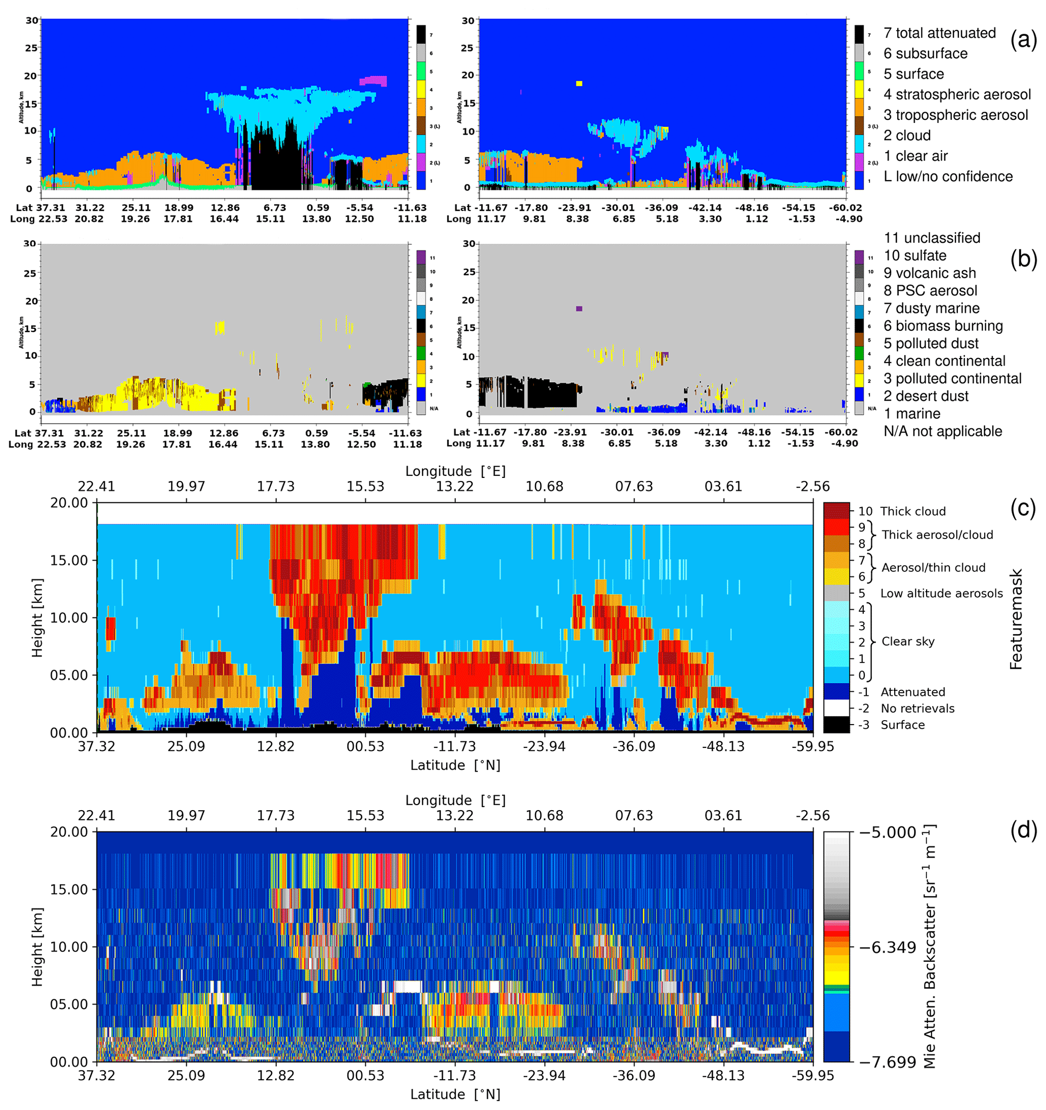
Figure 8 Comparison of Aeolus orbit 766 on 10 October 2018 and the collocated CALIPSO orbit (00:40:35 to 00:54:04 UTC) for feature masks. (a) CALIPSO vertical feature mask (version 4.51) standard nighttime hours. (b) CALIPSO aerosol subtype (version 4.51) standard nighttime hours. (c) Aeolus feature mask. (d) Aeolus Mie attenuated backscatter.

In general, the AEL-FM product compares well with the features of CALIPSO, but due to the time differences and large vertical bin sizes, we cannot expect the same features everywhere in the orbits. The cloud features often have some differences in height and geolocations. So in the evaluation of the extinction profiles, we only compared the aerosol extinction profiles between Aeolus and CALIPSO.

4.1.2 Extinction coefficient profiles

The particle extinction coefficient profiles from CALIPSO at 532 nm and Aeolus at 355 nm for the collocated orbits on 2 October 2018 are shown in Fig. 9. The aerosol extinction profiles from AEL-PRO were selected based on the AEL-PRO classification data (index = 103 for aerosols). The aerosol extinction image of CALIPSO looks cleaner than the extinction image of Aeolus. For the aerosols below 5 km, the two images have similar patterns and colours. So qualitatively, the CALIPSO and Aeolus aerosol extinction profiles are comparable. The Aeolus extinction profiles exhibit more low values in the range from 10⁻⁵ to 10⁻⁶ m⁻¹. The large extinction coefficients close to the tropopause are most likely from clouds and not aerosols. Because there is no cross-polar Mie channel in Aeolus, it is difficult to distinguish thin ice clouds from aerosols (much of the return from ice clouds is depolarized and thus not detected by Aeolus; this results in a lower apparent backscatter which decreases the contrast between less depolarizing elevated aerosols). The classification of cloud and aerosol is mainly based on the threshold applied to the backscatter coefficient. The images are plotted at 3 km horizontal resolution, but the actual resolution is roughly 90 km because of horizontal averaging. As shown in Fig. 9b, there are some high-resolution horizontal pixels but more horizontally averaged pixels. The extinction-to-backscatter (lidar) ratio profiles are also shown in Fig. 9d. The lidar ratio image looks more noisy than the extinction image because it is the ratio between two small values.

Figure 9 Comparison of Aeolus orbit 646 on 2 October 2018 and the collocated CALIPSO orbit for extinction coefficient profiles. (a) CALIPSO tropospheric aerosol extinction coefficient profiles (L2 5 km aerosol profiles v4.51), (b) Aeolus extinction coefficient profiles for all measurements, (c) Aeolus extinction coefficient profiles for tropospheric aerosols, and (d) Aeolus lidar ratios for tropospheric aerosols with extinction coefficients greater than $\mathrm{1.0}\times {\mathrm{10}}^{-\mathrm{5}}$ m⁻¹. The purple symbols mark the tropopause height in kilometres. The thin black contours indicate the atmospheric temperatures (units in K). The thick black line represents the surface height (units in km). CALIPSO extinction coefficients are at 532 nm. Aeolus extinction coefficients and lidar ratios are at 355 nm.

Figure 10 shows the comparison of aerosol extinction profiles between CALIPSO at 532 nm and Aeolus at 355 nm for orbit 766 on 10 October 2018. Figure 10b shows all Aeolus extinction profiles, both clouds and aerosols, for which there are lots of extinction coefficients greater than 10⁻³ m⁻¹. The total extinction profiles include the aerosol extinction profiles which are very similar to the CALIPSO aerosol extinction profiles. After the cloud-contaminated bins are removed, the Aeolus aerosol extinction profiles have similar colours to the CALIPSO extinction profiles. However, it clearly indicates that too many bins at the top of the aerosol plumes between 2.5 and 5 km are removed from the Aeolus extinction profiles. The aerosol extinction coefficients between 5 km and the tropopause height are also too large compared to the CALIPSO aerosol extinction profiles.

Figure 10 Comparison of Aeolus orbit 766 on 10 October 2018 and the collocated CALIPSO orbit for extinction coefficient profiles. (a) CALIPSO tropospheric aerosol extinction coefficient profiles (L2 5 km aerosol profiles v4.51), (b) Aeolus extinction coefficient profiles for all measurements, (c) Aeolus extinction coefficient profiles for tropospheric aerosols, and (d) Aeolus lidar ratios for tropospheric aerosols with extinction coefficients greater than $\mathrm{1.0}\times {\mathrm{10}}^{-\mathrm{5}}$ m⁻¹. The purple symbols mark the tropopause height in kilometres. The thin black contours indicate the atmospheric temperatures (units in K). The thick black line represents the surface height (units in km). CALIPSO extinction coefficients are at 532 nm. Aeolus extinction coefficients and lidar ratios are at 355 nm.

Figure 10d shows lots of large S values (in yellow colours) which are mostly related to cirrus clouds and dust. We have analysed the distribution of S for dust at latitudes of 15–30° N and altitude bins below 5 km and for smoke at latitudes of 10–25° S and altitude bins below 5 km. The aerosol types were taken from the CALIPSO aerosol subtype image (Fig. 8b). As shown in Fig. 11, the lidar ratios for the smoke and dust scenes have different distributions. The smoke lidar ratio has a peak close to 75 (72–78) sr, but the distribution is rather broad from 25 to 120 sr. The dust lidar ratio has a large peak close to 54 (48–60) sr and a second peak close to 102 sr. In AEL-PRO, the a priori of aerosol lidar ratio is 60 sr and depolarization 0.15. The retrievals are not sensitive to the a priori values.

Figure 11 Histogram of Aeolus lidar ratios for dust aerosols (latitudes of 15–30° N; height below 5 km) and smoke aerosols (latitudes of 10–25° S; height below 5 km) in orbit 766 on 10 October 2018. The aerosol types are selected based on the CALIPSO aerosol subtype in Fig. 8b.

Floutsi et al. (2023) reported that the Saharan dust has S of 53.5 ± 7.7 sr and a depolarization ratio of 0.244 ± 0.025; in this case, the effective S can be 1.646 times the true S. The smoke has S of 68.2 ± 7.4 sr and a depolarization ratio of 0.027 ± 0.013; the effective S can be 1.055 times the true S. We think the lidar ratios in Fig. 11 are reasonable compared to the Sahara dust and smoke lidar ratios.

To provide further insight into the differences between the Aeolus and CALIPSO extinction profiles, we selected three collocated extinction profiles at latitudes of 30, 15, and −9.5° N. The longitude differences in the CALIPSO and Aeolus orbits are within 1.0°. The profiles were selected at cloud-free regions, according to the extinction images. The CALIPSO extinction coefficients at 532 nm were interpolated at the middle of each Aeolus altitude bin. The uncertainties in the CALIPSO extinction coefficients (Extinction_Coefficient_Uncertainty_532) were also interpolated at the Aeolus altitude bins. Figure 12 shows these three collocated extinction profiles and is a magnified view of the extinction profile images. The Aeolus extinction profiles are the full profiles; clouds are not removed. We can see that the extinction profiles have good agreement if the clouds can be removed properly. Although some bins have clouds, it seems that the retrieved aerosol extinction profiles are not affected by the clouds in other bins.

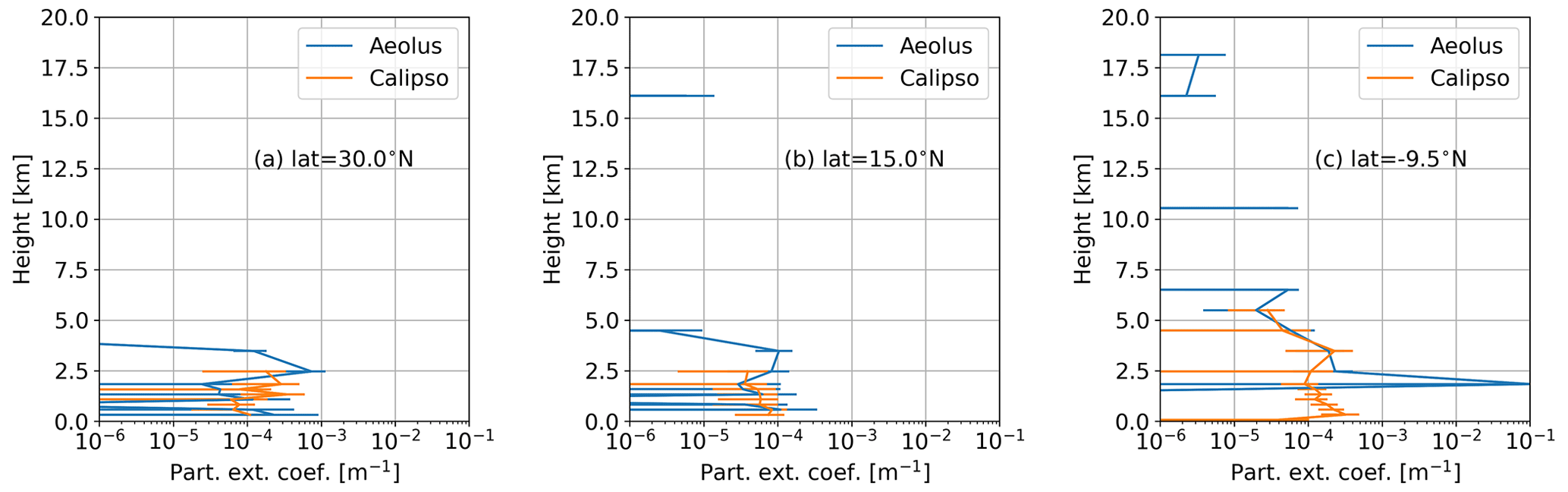
Figure 12 Comparison of Aeolus and CALIPSO extinction coefficient profiles (with error bars) at three locations in Aeolus orbit 766 on 10 October 2018 at latitudes (a) 30° N, (b) 15° N, and (c) −9.5° N, respectively, with the same data as in Fig. 10a and b. CALIPSO extinction coefficients are at 532 nm. Aeolus extinction coefficients are at 355 nm.

4.2 Comparison of monthly data

4.2.1 Aerosol extinction coefficient profiles

We processed the AEL-FM and AEL-PRO data in September and October 2018 and May and June 2019 because there were more aerosol events in the Sahara desert in the summer months. Unfortunately, there were missing data in CALIPSO in September 2018, and only half a month of Aeolus data were available in June 2019. So for the statistics, we use the collocated data, which include about 48 orbits in October 2018 and 43 orbits in May 2019. The Aeolus and CALIPSO extinction profiles are further selected for the region within the longitude range from −10 to 50° E and the latitude range from 0–30° N because the aerosol types are mainly dust in this region. The AEL-PRO aerosol extinction coefficient in each Aeolus altitude bin was compared with the CALIPSO aerosol extinction that was averaged in the Aeolus altitude bin and extrapolated to 355 nm.

The scatter plot of Aeolus and CALIPSO aerosol extinction coefficients for this region is shown in Fig. 13. The aerosol extinction coefficients show reasonable agreement between Aeolus and CALIPSO for October 2018 and May 2019. The data have large scatter which can be explained by the time differences and the possible evolution of aerosols. When selecting collocated extinction coefficients, some Aeolus aerosol extinction coefficients affected by clouds may be removed due to the absence of the CALIPSO aerosol extinction data in these bins.

Figure 13 Scatter plots of Aeolus tropospheric aerosol extinction coefficients versus CALIPSO tropospheric aerosol extinction coefficients for (a) October 2018 and (b) May 2019 in the region of −10 to 50° E longitude and 0 to 30° N latitude. The colour bar indicates the number of data points on a logarithmic scale. CALIPSO extinction coefficients are corrected to 355 nm. Aeolus extinction coefficients are at 355 nm.

Figure 14 shows the monthly mean extinction profiles with the same data as in Fig. 13 but averaged in vertical bins. Both profiles show that the dust layer is mainly below 5 km, and the extinction coefficient is larger at the ground surface and decreases at a higher altitude until 5 km. AEL-PRO extinction coefficient estimates are larger than CALIPSO close to the ground surface and above 7.5 km. This indicates the possible impact of clouds in the AEL-PRO aerosol profiles. It is also known that CALIPSO underestimates the aerosol extinction coefficients in the free troposphere due to limited sensitivity (Winker et al., 2013). In fact, the AEL-PRO results seem more consistent with, e.g., results from airborne lidar (Winker et al., 2013).

Figure 14 Monthly mean Aeolus and CALIPSO extinction coefficient profiles for collocated orbits, (a) October 2018 and (b) May 2019, in the region of −10 to 50° E longitude and 0 to 30° N latitude. Extinction coefficient profiles with AOT > 1 are excluded in both the CALIPSO and Aeolus extinction coefficient profiles. CALIPSO extinction coefficients are corrected to 355 nm. Aeolus extinction coefficients are at 355 nm.

4.2.2 Aerosol optical thickness

The Aeolus AOT was integrated using the aerosol extinction profile from the ground surface to 6 km but not the whole profile. As can be seen in the Aeolus aerosol extinction image, AEL-PRO often classified thin clouds as aerosols. In these 2 months, there were very few aerosols above 6 km based on the CALIPSO images, so we only used extinction profiles until 6 km to calculate the AOT. The CALIPSO AOT values at 532 nm were taken from the L2 product and then they were converted to the AOT at 355 nm.

Figures 15 and 16 show the AOT maps for October 2018 and May 2019 derived using AEL-PRO extinction profiles and the CALIPSO AOT, respectively. The CALIPSO AOT map clearly shows more aerosols over land and the transport of Saharan dust over ocean, with the AOT values mostly larger than 0.3. In the Aeolus AOT map over the land, the values are similar to the CALIPSO AOT. However, over the ocean, where CALIPSO shows lower AOT, Aeolus often shows high AOT. This suggests that some boundary layer clouds or cirrus were included in the Aeolus AOT calculations. Because of no depolarization data, AEL-PRO cannot really distinguish thin clouds and aerosols. The coarse vertical bin size may result in clouds and aerosols being in the same vertical bin.

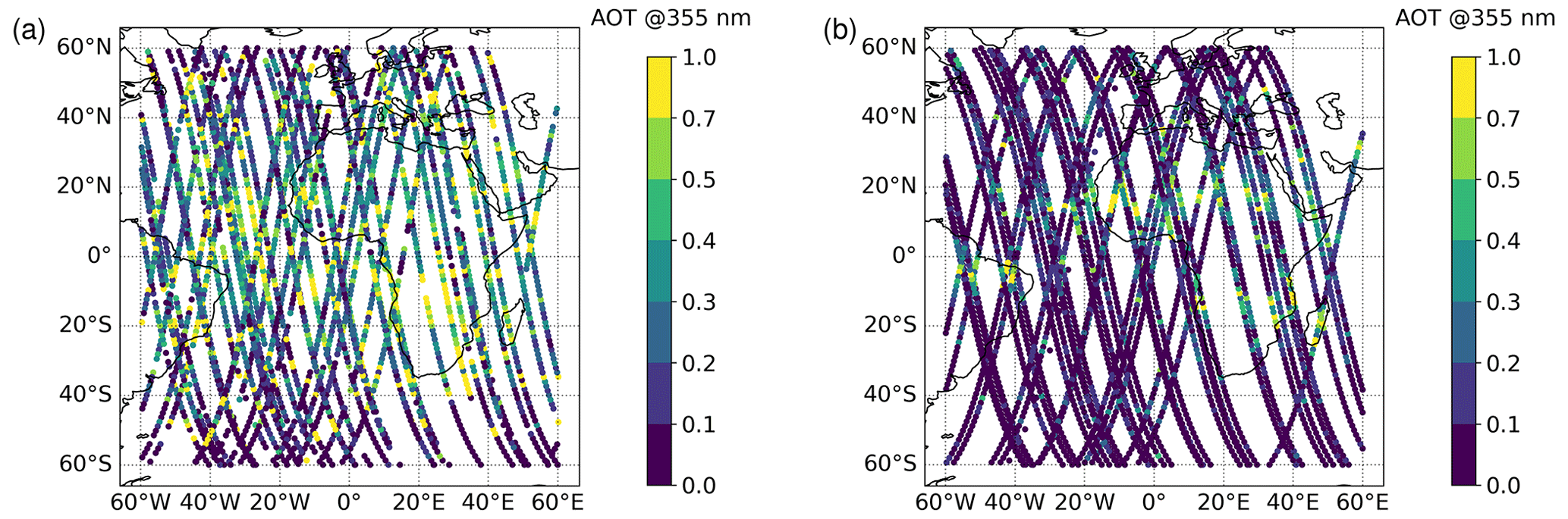
Figure 15 Maps of (a) Aeolus and (b) CALIPSO tropospheric aerosol optical thickness at 355 nm in October 2018.

Figure 16 Maps of (a) Aeolus and (b) CALIPSO tropospheric aerosol optical thickness at 355 nm in May 2019.

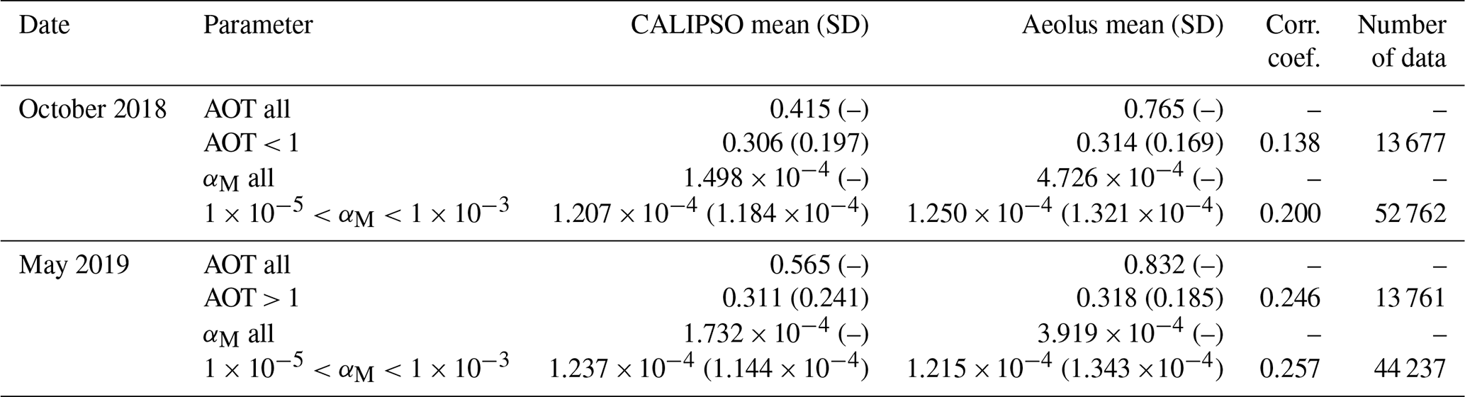
The Aeolus and CALIPSO AOT values are further selected for the region within the longitude range from −10 to 50° E and the latitude range from 0–30° N because the aerosol types are mainly dusts, and there are relatively high AOT values in this region. The scatter plot of Aeolus and CALIPSO AOT at 355 nm for this region is shown in Fig. 17. The Aeolus and CALIPSO AOTs have some correlations. The agreement is better at the small AOT than at the large AOT. It is possible that the small AOT represents background dust aerosols, which is more stable than the dust plumes with large AOT. If the AOT values larger than 1 are excluded, the mean Aeolus AOT is 0.314 (±0.169) in October 2018 and 0.318 (±0.185) in May 2019, and the mean CALIPSO AOT is 0.306 (±0.197) in October 2018 and 0.311 (±0.241) in May 2019. The results are summarized in Table 1.

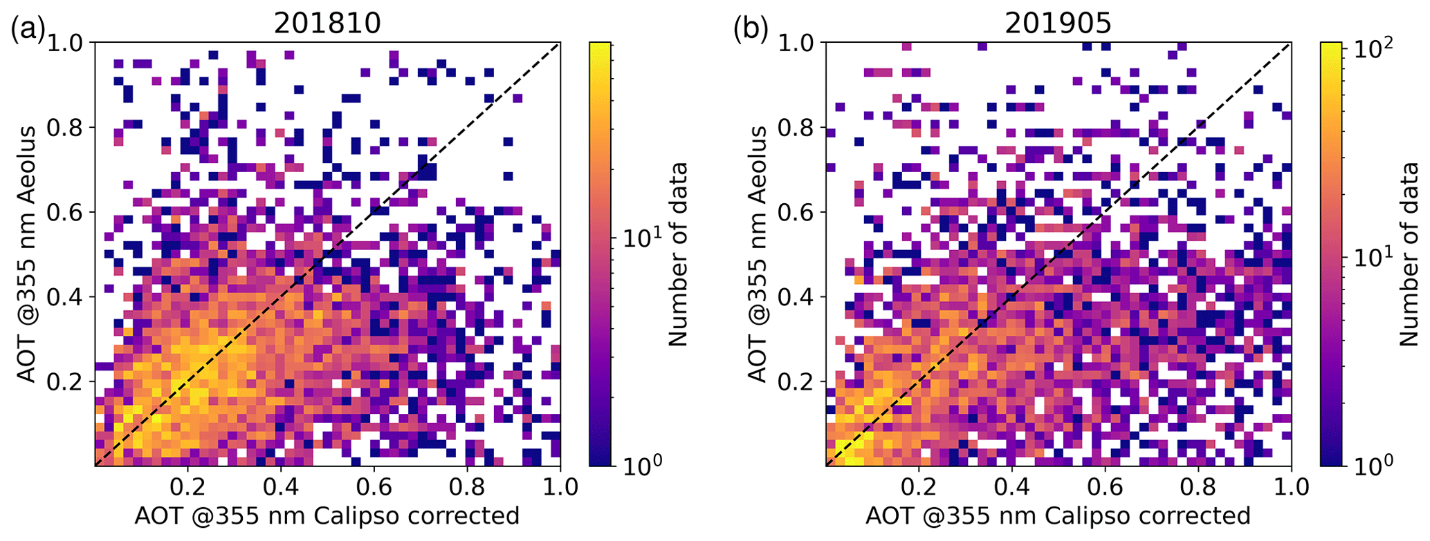
Figure 17 Scatter plots of Aeolus tropospheric aerosol optical thickness versus CALIPSO tropospheric aerosol optical thickness for (a) October 2018 and (b) May 2019 in the region of −10 to 50° E longitude and 0 to 30° N latitude. The colour bar indicates the number of data points on a logarithmic scale. CALIPSO AOTs are corrected to 355 nm. Aeolus AOTs are at 355 nm.

Table 1 Monthly mean AOT and extinction coefficient (α_M, unit m⁻¹) for CALIPSO and Aeolus at 355 nm in selected region for dust aerosols. Note that “Corr. coef.” stands for correlation coefficient. SD stands for standard deviation.

According to Floutsi et al. (2023), the Ångström coefficient is 0.1 ± 0.2 for Sahara dust, 0.2 ± 0.1 for central Asian dust, 0.1 ± 0.1 for Middle Eastern dust, 0.5 ± 0.5 for dust and marine, and 0.7 ± 0.4 for dust and pollution. So the Ångström coefficient we used is close to the dust and marine case. If we use the Ångström coefficient of 0.1 or 0.2, the CALIPSO extinction coefficient at 355 nm will be smaller. The conversion factor will be changed from 1.25 to 1.08 or 1.04.

5 Conclusions

The AEL-FM feature mask and AEL-PRO extinction profile products have been compared to the CALIPSO vertical feature mask and extinction profile products for desert dust aerosols over Africa using 2 months of collocated data in October 2018 and May 2019. Generally, Aeolus feature masks appear at similar altitude locations to the CALIPSO vertical feature masks, although there are 4 h time differences. The extinction profiles have good agreement for cloud-free aerosol extinction profiles. The monthly mean tropospheric extinction coefficients are about $\mathrm{1.2}\times {\mathrm{10}}^{-\mathrm{4}}$ m⁻¹; this is similar for Aeolus and CALIPSO if we limit the individual values between $\mathrm{1.0}\times {\mathrm{10}}^{-\mathrm{5}}$ and $\mathrm{1.0}\times {\mathrm{10}}^{-\mathrm{3}}$ m⁻¹. Without this limitation, the Aeolus monthly mean extinction coefficients are about 2–3 times larger than the CALIPSO extinction coefficients, which suggests contamination by thin clouds. The monthly mean AOT values are also similar between Aeolus and CALIPSO if the individual AOT values are limited to between $\mathrm{1.0}\times {\mathrm{10}}^{-\mathrm{6}}$ and 1. Without the limit of the AOT, the Aeolus monthly mean AOT values are 1.5 to 1.9 times larger than the CALIPSO AOT values in the selected dust aerosol region.

The separation of aerosols from clouds has to be improved in the Aeolus aerosol products. However, due to the missing cross-polar channel in the Aeolus measurements, there is consequently no depolarization ratio product. The lack of depolarization ratio information makes it difficult to separate aerosols and thin clouds. Also because of the large vertical bins and horizontal pixels, some bins may be partly filled with clouds. Without the depolarization ratio and true lidar ratio products, we cannot derive aerosol subtypes. We hope the cross-polar channel can be included in Aeolus-2 to provide better aerosol and cloud identification.

The AEL-FM and AEL-PRO products have been implemented and verified in the Aeolus Baseline 16 L2A product. We expect the AEL-FM and AEL-PRO products in L2A Baseline 16, and later baselines have a similar or better quality than the prototype products used in this analysis.

In spite of the difficulties in separating aerosol and cloud in the Aeolus observations, both the Aeolus feature mask and extinction coefficient profile products show good agreement with the CALIPSO L2 products, which gives us confidence in the A-FM and A-PRO products to be produced by EarthCARE. It is expected that the addition of a depolarization channel, better SNR, and a better resolution for ATLID will result in an improved ability to separate clouds and aerosols.

Appendix A: Verification of AEL-FM and AEL-PRO in Aeolus L2A products

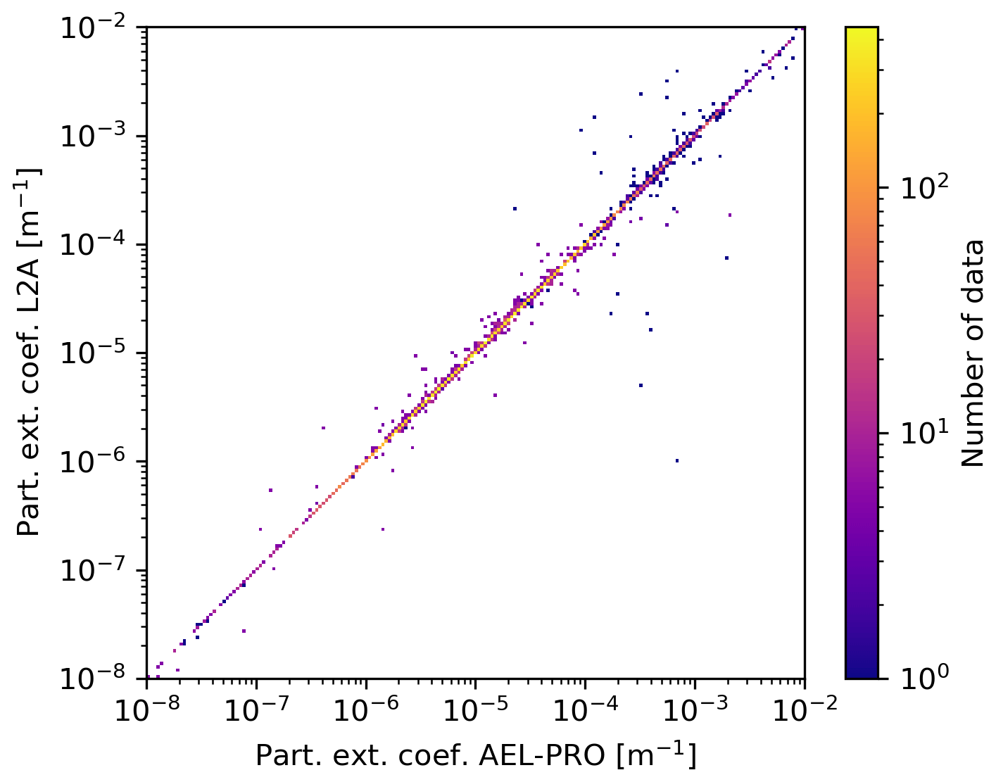
The AEL-FM and AEL-PRO products in L2A were verified with the prototype products during the implementation in L2A processor from versions 3.14 to 3.17 (Baselines 14 to 17). The products were also verified during the third and fourth data reprocessing. We found that the L2A and prototype products are almost identical for most orbits. Figures A1 and A2 show an example of the verification of the prototype and L2A AEL-FM and AEL-PRO products for L2A version 3.16.4 (Baseline 16). Figure A3 shows a scatter plot of the L2A AEL-PRO extinction coefficients versus the prototype. There are only a few data points with large differences between L2A and the prototype extinction coefficients.

Figure A1 Comparison of the AEL-FM featuremask in (a) L2A with (b) the prototype product for orbit 23453 on 9 September 2022. L2A version 3.16.4 (Baseline 16) is used.

Figure A2 Comparison of AEL-PRO extinction coefficient profiles in (a) L2A and (b) the prototype for orbit 23453 on 9 September 2022. L2A version 3.16.4 (Baseline 16) is used. The purple symbols mark the tropopause height in kilometres. The thin black contours indicate the atmospheric temperatures (units in K). The thick black line represents the surface height (units in km).

Figure A3 Scatter plot of AEL-PRO extinction coefficients in L2A versus the prototype for orbit 23453 on 9 September 2022, with the same data as in Fig. A2. The colour bar indicates the number of data points on a logarithmic scale.