Estimating the turbulent kinetic energy dissipation rate from one-dimensional velocity measurements in time

The turbulent kinetic energy dissipation rate is one of the most important quantities characterizing turbulence. Experimental studies of a turbulent flow in terms of the energy dissipation rate often rely on one-dimensional measurements of the flow velocity fluctuations in time. In this work, we first use direct numerical simulation of stationary homogeneous isotropic turbulence at Taylor-scale Reynolds numbers $\mathrm{74}\le R_{\mathit{\lambda }}\le \mathrm{321}$ to evaluate different methods for inferring the energy dissipation rate from one-dimensional velocity time records. We systematically investigate the influence of the finite turbulence intensity and the misalignment between the mean flow direction and the measurement probe, and we derive analytical expressions for the errors associated with these parameters. We further investigate how statistical averaging for different time windows affects the results as a function of R_λ. The results are then combined with Max Planck Variable Density Turbulence Tunnel hot-wire measurements at $\mathrm{147}\le R_{\mathit{\lambda }}\le \mathrm{5864}$ to investigate flow conditions similar to those in the atmospheric boundary layer. Finally, practical guidelines for estimating the energy dissipation rate from one-dimensional atmospheric velocity records are given.

1 Introduction

Turbulence is fundamental to many natural and engineering processes, such as transport of heat and moisture in the Earth's atmosphere (e.g., Wyngaard, 1992; Garratt, 1994; Muschinski and Lenschow, 2001; Fairall and Larsen, 1986; Hsieh and Katul, 1997), wind energy conversion (Smalikho et al., 2013), entrainment and mixing (e.g., Warhaft, 2000; Sreenivasan, 2004; Deshpande et al., 2009; Gerber et al., 2008, 2013; Siebert et al., 2013; Fodor and Mellado, 2020), and warm rain initiation (e.g., Shaw, 2003; Devenish et al., 2012; Pumir and Wilkinson, 2016; Li et al., 2020), to name just a few. In three-dimensional turbulence, the kinetic energy is typically injected into the flow at the largest scales and is successively transferred to smaller eddies by means of the direct energy cascade. At the smallest scales characterized by the Kolmogorov length scale (or the dissipation scale) η_K, kinetic energy is dissipated by viscous effects at the energy dissipation rate (a list of all the parameters and symbols used in this study can be found in Tables A1 and A2). The energy dissipation rate is one of the most fundamental quantities in turbulence and is used to estimate many relevant features of a turbulent flow, such as the Kolmogorov length scale η_K; the Taylor microscale λ; the Taylor-scale Reynolds number R_λ; and, by means of dimensional estimates, the energy injection scale.

The instantaneous energy dissipation field ϵ₀(x,t), which is a function of the fluid kinematic viscosity ν and the velocity gradient tensor, is highly intermittent with strong small-scale fluctuations (Pope, 2000; Davidson, 2015, and references therein), which are at the core of the intermittency problem in turbulence (Sreenivasan and Antonia, 1997; Muschinski et al., 2004; Buaria et al., 2019). By “instantaneous” we want to emphasize here that ϵ₀ is the energy dissipation rate at one point in space and time within the flow. It also plays an important role in turbulent mixing in reacting flows (e.g., Sreenivasan, 2004; Hamlington et al., 2012; Sreenivasan, 2019) or turbulence-induced rain initiation in warm clouds (Devenish et al., 2012). ϵ₀(x,t), however, is extremely difficult to measure experimentally because it requires complete knowledge of the three-dimensional velocity field with spatial and temporal resolution that can resolve scales smaller than or at least comparable to the Kolmogorov scales.

Apart from the instantaneous dissipation field ϵ₀(x,t), the energy dissipation in a turbulent flow can be statistically described by either the local or global mean energy dissipation rate, which are both important. Local volume averages of the instantaneous dissipation field 〈ϵ₀〉_R and related surrogates, e.g., diagonal or off-diagonal components of the velocity gradient, can capture intermittency of turbulence (Lefeuvre et al., 2014; Almalkie and de Bruyn Kops, 2012, and references therein). The local volume averages of the dissipation field converge to the global mean energy dissipation rate 〈ϵ〉 for statistically converged sampling. The mean dissipation rate 〈ϵ〉 can be used to parameterize the statistics of statistically homogeneous and locally isotropic turbulence based on Kolmogorov's phenomenology (K41) (Kolmogorov, 1941). Note that even if the global mean energy dissipation rate 〈ϵ〉 is known, it is also of high interest to know how locally averaged dissipation rates 〈ϵ₀〉_R differ from the global mean energy dissipation rate 〈ϵ〉. For example, the local dissipation rate determines whether droplets in a cloud behave as tracer or inertial particles, which in turn can affect the probability of collision and coalescence of the droplets and thus the likelihood of precipitation initiation (e.g., see Shaw, 2003).

For a statistically stationary homogeneous isotropic (SHI) turbulent flow, 〈ϵ〉 can be estimated from time-dependent single-point one-dimensional velocity measurements through different methods, such as longitudinal or transverse velocity gradients (Wyngaard and Clifford, 1977; Elsner and Elsner, 1996; Antonia, 2003; Siebert et al., 2006, among others), inertial-range scaling laws comprising the famous $\mathrm{4}/\mathrm{5}$ law (Kolmogorov, 1941, 1991; Muschinski et al., 2001), counting zero crossings of the velocity fluctuation time series (Sreenivasan et al., 1983; Wacławczyk et al., 2017), or dimensional arguments (e.g., Taylor, 1935; McComb et al., 2010; Vassilicos, 2015). These methods usually invoke Taylor's hypothesis to map temporal signals onto spatial signals, which requires a sufficiently small turbulence intensity. The turbulence intensity is defined as the ratio of the root mean square velocity fluctuations ${\mathit{\sigma }}_{u^{\prime }}$ to the mean velocity U. When all of these criteria are met, single-point velocity measurements with hot-wire anemometers at a high temporal resolution have been shown to be suitable for accurately estimating the global energy dissipation rate (see also below) (Lewis et al., 2021; Sinhuber, 2015; Elsner and Elsner, 1996; Antonia, 2003; Frehlich et al., 2003). However, in atmospheric flows, the assumption of ideal stationary homogeneous isotropic turbulence needs to be considered very carefully, as, for example, thermals change in local weather conditions, and of course the diurnal cycle may lead to non-stationarity and inhomogeneity.

Then the global mean energy dissipation rate 〈ϵ〉 is not representative, as the turbulence can be highly time- and space-dependent even at the energy injection scales. As a result, one needs to calculate a local 〈ϵ₀〉_τ and 〈ϵ₀〉_R, respectively, based on velocity statistics for a properly chosen averaging window τ in time and R in space, which is short enough for resolving the temporal or spatial variations but also long enough to obtain statistically representative values with acceptable systematic and/or random errors (e.g., Wyngaard, 1992; Lenschow et al., 1994). Therefore, a conflict arises with respect to the averaging time between resolving small-scale features of a turbulent flow and statistical convergence under non-stationary and inhomogeneous conditions.

In the case of atmospheric flows, in situ measurements made via airborne (e.g., Malinowski et al., 2013; Siebert et al., 2006, 2013; Muschinski et al., 2004; Frehlich et al., 2004; Nowak et al., 2021; Dodson and Small Griswold, 2021) as well as ground-based (e.g., Chamecki and Dias, 2004; O'Connor et al., 2010; Risius et al., 2015; Siebert et al., 2015) platforms can typically only resolve the coarse-grained time series of the local mean energy dissipation rate 〈ϵ₀〉_τ. However, it remains unclear how large the errors in estimating the coarse-grained time series of the local mean energy dissipation rate are due to individual choices of the averaging window, since there is currently no high-resolution three-dimensional velocity measurement available during in situ measurements to serve as the ground truth. In the absence of a ground-truth reference, the comparison between different methods was used as the next best benchmark for validity of a given method (Siebert et al., 2010; Wacławczyk et al., 2020; Siebert et al., 2006; Risius et al., 2015; Wacławczyk et al., 2017), which in some cases makes the interpretation of the data difficult due to the large discrepancies between the estimates obtained by different methods. As an example, Wacławczyk et al. (2020) found deviations of about 5 %–50 % with respect to estimating the mean energy dissipation rate depending on the method and averaging windows using synthetic data modeled via a von Kármán spectrum. Another example is the work of Akinlabi et al. (2019), who found that estimates of the mean energy dissipation rate by one-dimensional longitudinal velocity can differ by a factor of 2 to 3 from those calculated using direct numerical simulations (DNSs), depending on the method used.

Our literature review indicates that a systematic investigation is still needed to fully understand how the choice of averaging window, analysis methods, turbulence intensity and large-scale random flow velocities can influence estimating the mean energy dissipation rate and its deviations from the instantaneous energy dissipation rate. To this end, we systematically benchmark different techniques available in the literature using fully resolved DNS of statistically stationary, homogeneous, isotropic turbulence. Since the full dissipation field is available from DNS, this approach provides a ground-truth reference for comparisons with various estimation techniques. To bridge the gap between typical R_λ of DNS and atmospheric flows, we use high-resolution measurements of the longitudinal velocity components of the Variable Density Turbulence Tunnel (VDTT) (Bodenschatz et al., 2014; Sinhuber, 2015; Küchler et al., 2019) at various Taylor-scale Reynolds numbers R_λ between 140 and 6000. The impact of turbulence intensity, large-scale random-sweeping velocities, the size of the averaging window, the Reynolds number and also possible experimental imperfections such as anemometer misalignment are investigated in detail. Our work aims to be a step towards the goal of extracting the time-dependent energy dissipation rate from non-ideal naturally occurring turbulent flows, mitigating the impact of non-ideal features of the flow, e.g., anisotropy or inhomogeneity. In Sect. 2, we first define the central statistical quantities and the individual methods for estimating the energy dissipation rate in detail. An analysis of the individual methods including discrepancies, errors due to finite turbulence intensity and alignment errors are discussed in Sect. 3 followed by a summary of our findings.

2 Methods

Suppose $\mathit{u}(\mathit{x},t)=u_{\mathrm{1}}(\mathit{x},t){\mathit{e}}_{\mathrm{1}}+u_{\mathrm{2}}(\mathit{x},t){\mathit{e}}_{\mathrm{2}}+u_{\mathrm{3}}(\mathit{x},t){\mathit{e}}_{\mathrm{3}}$ denotes the three-dimensional velocity vector of the turbulent flow, where $\mathit{x}=x_{\mathrm{1}}{\mathit{e}}_{\mathrm{1}}+x_{\mathrm{2}}{\mathit{e}}_{\mathrm{2}}+x_{\mathrm{3}}{\mathit{e}}_{\mathrm{3}}$ is the position and t is the time. We assume that the streamwise direction of the global mean flow U is in the direction of e₁ such that U=Ue₁ is (by definition) constant in space and time. We refer to e₁ as the longitudinal direction and the components normal to that, i.e., e₂ and e₃, as the transverse directions of the flow. As mentioned earlier, many experimental setups record only a one-dimensional flow velocity at one location and as a function of time. We consider this one-dimensional velocity time record to be in the longitudinal flow direction unless otherwise stated, e.g., when the probe misalignment is investigated. In the following, we first introduce different averaging principles that can be used to analyze turbulence statistics and Taylor's frozen hypothesis, and then we present the commonly used methods for extracting the energy dissipation rate. An introduction of the basic statistical description of turbulent flows is provided in the Appendix (Appendix A) for the sake of completeness.

2.1 On averaging, Reynolds decomposition and Taylor's hypothesis

Most methods used to retrieve the dissipation rate require spatially resolved velocity statistics, although the velocity is recorded only at a single point and as a function of time in many experiments. Therefore, prior to estimating the energy dissipation rate, the one-dimensional velocity time record should first be mapped onto a spatially resolved velocity field. This is achieved by invoking Taylor's hypothesis (Taylor, 1938), which requires a Reynolds decomposition of the velocity time record by separating the velocity fluctuations from the mean velocity. To perform the Reynolds decomposition, we first have to clarify what is meant by the mean velocity.

Generally, we have to distinguish between the global mean velocity $\mathit{U}=\langle \mathit{u}(\mathit{x},t)\rangle =U{\mathit{e}}_{\mathrm{1}}$, the volume-averaged velocity 〈u(x,t)〉_R over a sphere of radius R (for one-dimensional data 〈⋅〉_R denotes spatial averages over a window of size R), the time-averaged velocity 〈u(x,t)〉_τ over a time interval τ and the ensemble-averaged velocity 〈u(x,t)〉_N over N realizations (Wyngaard, 2010; Pope, 2000, among others). In this work, 〈⋅〉 denotes the global mean, i.e., for infinitely large averaging windows in time or space. Thus, U is by definition independent of time and space, which in reality is valid only when u(x,t) is statistically stationary and homogeneous. Implicitly, $\langle \mathit{u}(\mathit{x},t){\rangle }_R=\mathrm{3}/\left(\mathrm{4}\mathit{\pi }{R}^{\mathrm{3}}\right){\iiint }_{\mathrm{0}}^R\mathrm{d}\mathit{x}\mathit{u}(\mathit{x},t)$ and $\langle \mathit{u}(\mathit{x},t){\rangle }_{\mathit{\tau }}=\frac{\mathrm{1}}{\mathit{\tau }}{\int }_{-\mathit{\tau }/\mathrm{2}}^{\mathit{\tau }/\mathrm{2}}\mathrm{d}{t}^{\prime }\mathit{u}(\mathit{x},t^{\prime })$ are, respectively, local volume and time averages, as both R and τ are typically finite. In the limit of R, τ→∞, 〈u(x,t)〉_R and 〈u(x,t)〉_τ tend toward U. For repeatable experiments where identical experimental conditions are guaranteed, 〈u(x,t)〉_N tends toward U when N→∞.

The mean of a one-dimensional velocity time record in the longitudinal direction U_τ here is defined by

$$\begin{array}{}\text{(1)}& U_{\mathit{\tau }}=\langle u_{\mathrm{1}}\left(t\right){\rangle }_{\mathit{\tau }}={\displaystyle \frac{\mathrm{1}}{\mathit{\tau }}}\underset{-\mathit{\tau }/\mathrm{2}}{\overset{\mathit{\tau }/\mathrm{2}}{\int }}\mathrm{d}{t}^{\prime }{u}_{\mathrm{1}}\left(t^{\prime }\right)\end{array}$$

such that the global mean $U={lim}_{\mathit{\tau }\to \mathrm{\infty }}{U}_{\mathit{\tau }}$, where τ is the averaging window. It should be noted that the global mean of the transverse velocity will be equal to zero; i.e., $\langle u_{\mathrm{2},\mathrm{3}}\left(t\right){\rangle }_{\mathit{\tau }}=\mathrm{0}$ when τ→∞, since here it is assumed that they are orthogonal to the mean flow direction. According to the Reynolds decomposition, the longitudinal velocity time record is composed of the mean velocity U and the random velocity fluctuation component $u_{\mathrm{1}}^{\prime }\left(t\right)=u_{\mathrm{1}}\left(t\right)-U$ so that the mean of the longitudinal velocity fluctuations $\langle u_{\mathrm{1}}^{\prime }\left(t\right)\rangle =\mathrm{0}$.

In certain circumstances, it is possible to map $u_{\mathrm{1}}^{\prime }\left(t\right)$ from time to space coordinates by applying Taylor's (frozen-eddy) hypothesis (Taylor, 1938; Wyngaard, 2010), which relates temporal and spatial velocity statistics. Taylor (1938) argues that eddies can be regarded as frozen in time if they are passing the probing volume much faster than they evolve in time. This is the case if the turbulence intensity $I={\mathit{\sigma }}_{u_{\mathrm{1}}^{\prime }}/U$ is much smaller than unity, i.e., I≪1, where ${\mathit{\sigma }}_{u_{\mathrm{1}}^{\prime }}=\langle u_{\mathrm{1}}^{\prime \mathrm{2}}{\rangle }^{\mathrm{1}/\mathrm{2}}$ is the root mean square (rms) velocity fluctuation. Then, the series of time lags $\mathrm{\Delta }t=t-t_{\mathrm{0}}$ relative to the start time t₀ is mapped onto a distance vector with $\mathit{x}={\mathit{x}}_{\mathrm{0}}+U\mathrm{\Delta }t{\mathit{e}}_{\mathrm{1}}$ (Taylor, 1938), where x₀ is the initial position at time t₀. This approach is found to be reliable for I≲0.25 (Nobach and Tropea, 2012; Wilczek et al., 2014; Risius et al., 2015), while it has been shown to fail when I>0.5 (Willis and Deardorff, 1976). The application of Taylor's hypothesis is inaccurate in the case of large-scale variations in the velocity fluctuation field comparable with the mean velocity, which are known as “random-sweeping velocity” (Kraichnan, 1964; Tennekes, 1975). Complicating the estimation of the mean velocity, random-sweeping causes the mean energy dissipation rate to be consistently overestimated (Lumley, 1965; Wyngaard and Clifford, 1977).

One way to cope with non-stationary velocity time records is to evaluate the mean velocity for a subset of this signal. If the averaging time τ is finite, the time average U_τ may differ from the mean velocity U, causing a systematic bias in the subsequent data analysis. The estimation variance of the time average U_τ can be analytically expressed as (Wyngaard, 2010; Pope, 2000, among others)

$$\begin{array}{}\text{(2)}& \langle (U_{\mathit{\tau }}-U{)}^{\mathrm{2}}\rangle \approx {\displaystyle \frac{\mathrm{2}\langle u_{\mathrm{1}}^{\prime \mathrm{2}}\rangle T}{\mathit{\tau }}},\end{array}$$

where T is the integral timescale and $\langle u_{\mathrm{1}}^{\prime \mathrm{2}}\rangle$ the variance of the velocity time series. Notably, the size of the averaging window has to be large enough such that it fulfills $\langle u_{\mathrm{1}}^{\prime }\left(t\right){\rangle }_{\mathit{\tau }}\approx \mathrm{0}$ to apply the Reynolds decomposition.

2.2 Estimating the energy dissipation rate

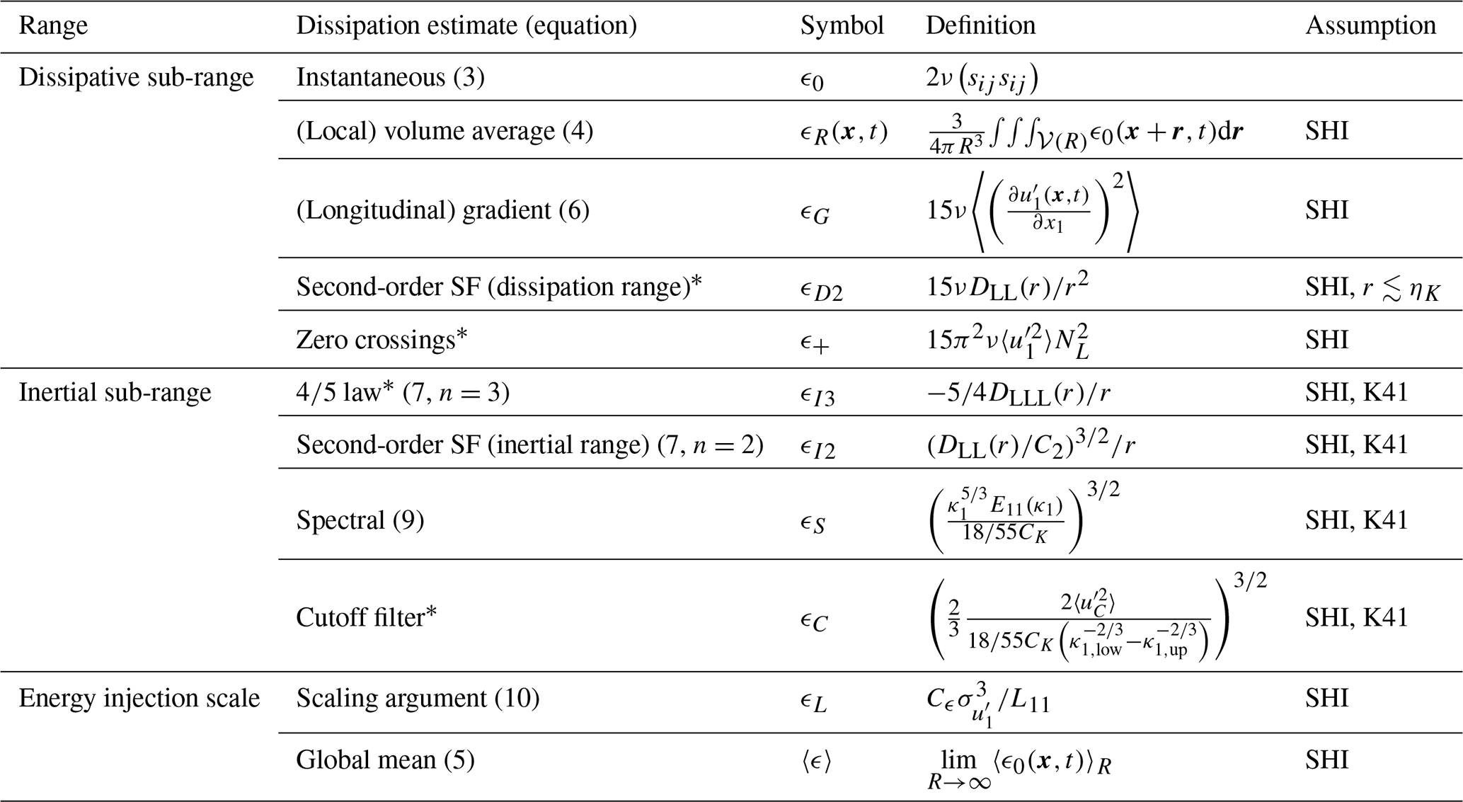
The energy dissipation rate can be derived from various statistical quantities. A non-exhaustive list of the most common methods applicable to single-point measurements is shown in Table 1. Details of selected methods considered in this study are presented in the following subsections. If not explicitly mentioned, the averages denoted with 〈⋅〉 are defined globally.

Table 1 Various definitions of the energy dissipation rate from the dissipative and inertial sub-range to the energy injection range. Here, the definitions for various dissipation estimates are given in the space or wavenumber domain, where ν is the viscosity, s_ij is the velocity fluctuation strain-rate tensor, R is the radius of the averaging volume 𝒱(R) (window size for one-dimensional data), $u_{\mathrm{1}}^{\prime }\left(\mathit{x}\right)$ is the longitudinal velocity fluctuation field along e₁, D_L…L(r) is the nth-order longitudinal structure function (SF) for distance r, $\langle u_{\mathrm{1}}^{\prime \mathrm{2}}\rangle$ is the variance of $u_{\mathrm{1}}^{\prime }\left(\mathit{x}\right)$, ${\mathit{\sigma }}_{u_{\mathrm{1}}^{\prime }}$ is the standard deviation of $u_{\mathrm{1}}^{\prime }\left(\mathit{x}\right)$, N_L is the number of zero crossings of a velocity fluctuation signal per unit length, C₂≈2, E₁₁(κ₁) is the one-dimensional energy spectrum with wavenumber κ₁, C_K≈1.5, $\langle u_C^{\prime \mathrm{2}}\rangle$ is the variance of a band-pass-filtered signal for wavenumbers ${\mathit{\kappa }}_{\mathrm{1}}\in [{\mathit{\kappa }}_{\mathrm{1},\mathrm{low}},{\mathit{\kappa }}_{\mathrm{1},\mathrm{up}}]$, C_ϵ is the dissipation constant, L₁₁ is the longitudinal integral scale and η_K is the Kolmogorov length scale. Dissipation estimates indicated with ^* are not considered in detail in this work. The assumptions of stationarity (S), homogeneity (H), local isotropy (I) and Kolmogorov's second similarity hypothesis from 1941 (K41) are represented by their individual abbreviations. References are given in the corresponding sections in the main text.

2.2.1 Dissipative sub-range

Proceeding from the Navier–Stokes equations for an incompressible Newtonian fluid, the instantaneous energy dissipation rate is given by 2ν(S_ijS_ij) (e.g., Pope, 2000; Davidson, 2015). As the velocity gradients are dominated by small-scale fluctuations, turbulent kinetic energy is dissipated into heat at small scales. Therefore, the contribution of large-scale variations in the velocity is small compared with the contribution of the small scales (Pope, 2000; Elsner and Elsner, 1996). Hence, the instantaneous energy dissipation rate can be defined in terms of the velocity fluctuations only, i.e., replacing S_ij with the fluctuation strain-rate tensor $s_{ij}=(\partial u_i^{\prime }(\mathit{x},t)/\partial x_j+\partial u_j^{\prime }(\mathit{x},t)/\partial x_i)/\mathrm{2}$ (Pope, 2000):

$$\begin{array}{}\text{(3)}& {\mathit{ϵ}}_{\mathrm{0}}(\mathit{x},t)=\mathrm{2}\mathit{\nu }\left(s_{ij}{s}_{ij}\right).\end{array}$$

Averaged over a sphere with radius R and volume 𝒱(R), the (local) volume average of the instantaneous energy dissipation rate is (Pope, 2000)

$$\begin{array}{}\text{(4)}& {\mathit{ϵ}}_R(\mathit{x},t)=\langle {\mathit{ϵ}}_{\mathrm{0}}(\mathit{x},t){\rangle }_R={\displaystyle \frac{\mathrm{3}}{\mathrm{4}\mathit{\pi }{R}^{\mathrm{3}}}}\underset{\mathcal{V}\left(R\right)}{\iiint }{\mathit{ϵ}}_{\mathrm{0}}(\mathit{x}+\mathit{r},t)\mathrm{d}\mathit{r}.\end{array}$$

The local volume average ϵ_R(x,t) converges to the global mean energy dissipation rate if R tends toward infinity (Pope, 2000):

$$\begin{array}{}\text{(5)}& \langle \mathit{ϵ}\rangle =\underset{R\to \mathrm{\infty }}{lim}\langle {\mathit{ϵ}}_{\mathrm{0}}(\mathit{x},t){\rangle }_R.\end{array}$$

In experiments, it is often not possible to measure ϵ₀(x,t). Under the assumption of statistically homogeneous and isotropic turbulence, the volume- and time-averaged energy dissipation rate are typically inferred from one-dimensional surrogates (Taylor, 1935; Elsner and Elsner, 1996; Siebert et al., 2006; Almalkie and de Bruyn Kops, 2012; Champagne, 1978; Donzis et al., 2008, among others), such as from the longitudinal velocity gradient (hence, the subscript G):

$$\begin{array}{}\text{(6)}& \begin{array}{rl}{\mathit{ϵ}}_G& =-\mathrm{15}\mathit{\nu }\underset{\left|\mathit{r}\right|\to \mathrm{0}}{lim}{\partial }_{r_{\mathrm{1}}}^{\mathrm{2}}{R}_{\mathrm{11}}(\mathit{r},t)=\mathrm{15}\mathit{\nu }〈{\left({\displaystyle \frac{\partial u_{\mathrm{1}}^{\prime }(\mathit{x},t)}{\partial x_{\mathrm{1}}}}\right)}^{\mathrm{2}}〉\\ & ={\displaystyle \frac{\mathrm{15}\mathit{\nu }}{U^{\mathrm{2}}}}〈{\left({\displaystyle \frac{\partial u_{\mathrm{1}}^{\prime }\left(t\right)}{\partial t}}\right)}^{\mathrm{2}}〉,\end{array}\end{array}$$

where the mapping between space and time domains is possible by applying Taylor's hypothesis if ${\mathit{\sigma }}_{u_{\mathrm{1}}^{\prime }}/U\ll \mathrm{1}$ and R₁₁ is the longitudinal component of the velocity covariance tensor defined in Eq. (A1) (Siebert et al., 2006; Muschinski et al., 2004). The relationship shown in Eq. (6) is often called the “direct” method in the literature (e.g., Muschinski et al., 2004; Siebert et al., 2006) and requires a spatial resolution higher than the Kolmogorov length scale η_K to be accurate within ∼10 % (see Fig. A8).

2.2.2 Inertial sub-range: structure functions

Kolmogorov's second similarity hypothesis from 1941 (Kolmogorov, 1941) provides another method for estimating the energy dissipation rate in the inertial range. Based on the inertial-range scaling of the nth-order longitudinal structure function, the mean energy dissipation rate can be calculated by (Pope, 2000)

$$\begin{array}{}\text{(7)}& D_{\mathrm{L}\mathrm{\dots }\mathrm{L}}\left(r\right)=C_n({\mathit{ϵ}}_{\mathrm{In}}r{)}^{{\mathit{\zeta }}_n}\iff {\mathit{ϵ}}_{\mathrm{In}}={\left({\displaystyle \frac{D_{\mathrm{L}\mathrm{\dots }\mathrm{L}}\left(r\right)}{C_n}}\right)}^{\mathrm{1}/{\mathit{\zeta }}_n}{\displaystyle \frac{\mathrm{1}}{r}},\end{array}$$

where C_n is a constant, e.g., C₂≈2 (Pope, 2000), and ${\mathit{\zeta }}_n=n/\mathrm{3}$ according to K41 by dimensional analysis. In practice, ϵ_I2 (Table 1) is retrieved by fitting either a constant to the compensated longitudinal second-order structure function D_LL(r), n=2 in Eq. (7), or a power law ($\propto r^{\mathrm{2}/\mathrm{3}}$) to the inertial range of D_LL, defined in Eq. (A3), if the inertial range is pronounced over at least a decade. Accounting for intermittency, the scaling exponent of the nth-order structure function is modified to ${\mathit{\zeta }}_n=\frac{n}{\mathrm{3}}\left[\mathrm{1}-\frac{\mathrm{1}}{\mathrm{6}}\mathit{\mu }(n-\mathrm{3})\right]$, where μ is the internal intermittency exponent (Kolmogorov, 1962; Obukhov, 1962; Pope, 2000). The inertial range is bounded by the energy injection scale L at large scales and by the dissipation range at small scales. That is why the fit range has to be chosen such that ${\mathit{\eta }}_K\ll r\ll L$. If the inertial range is not sufficiently pronounced, the extended self-similarity may be used to extend the inertial range (Benzi et al., 1993b, a). Otherwise, ϵ_I2 can also be approximated by the maximum of Eq. (7) (for n=2) within the same range as before. This is possible because the maximum lies on the plateau in the case of a perfect K41 inertial-range scaling.

In the inertial range, the transverse second-order structure function D_NN(r) is equal to $\mathrm{4}{D}_{\mathrm{LL}}\left(r\right)/\mathrm{3}$ in a coordinate system where r=re₁ is parallel to the longitudinal flow direction (Pope, 2000), highlighting the importance of the measurement direction.

2.2.3 Inertial sub-range: spectral method

According to K41 (Kolmogorov, 1941), the inertial sub-range of the energy spectrum function scales as $E\left(\mathit{\kappa }\right)\propto \langle \mathit{ϵ}{\rangle }^{\mathrm{2}/\mathrm{3}}{\mathit{\kappa }}^{-\mathrm{5}/\mathrm{3}}$ with the wavenumber κ by dimensional analysis. In isotropic turbulence, the energy spectrum function can be converted into a one-dimensional energy spectrum E₁₁(κ₁); see Eq. (A7). The wavenumber space is not directly accessible from one-dimensional velocity time records. Relying on Taylor's hypothesis, the one-dimensional energy spectrum E₁₁(κ₁) transforms into the frequency domain with $F_{\mathrm{11}}\left(f\right)=\mathrm{2}\mathit{\pi }{E}_{\mathrm{11}}\left({\mathit{\kappa }}_{\mathrm{1}}\right)/U$, where ${\mathit{\kappa }}_{\mathrm{1}}=\mathrm{2}\mathit{\pi }f/U$ (e.g., Wyngaard and Clifford, 1977; Oncley et al., 1996), yielding

$$\begin{array}{}\text{(8)}& F_{\mathrm{11}}\left(f\right)={\displaystyle \frac{\mathrm{18}}{\mathrm{55}}}{C}_K{\left({\displaystyle \frac{U}{\mathrm{2}\mathit{\pi }}}{\mathit{ϵ}}_S\right)}^{\mathrm{2}/\mathrm{3}}{f}^{-\mathrm{5}/\mathrm{3}},\end{array}$$

which yields

$$\begin{array}{}\text{(9)}& {\mathit{ϵ}}_S={\displaystyle \frac{\mathrm{2}\mathit{\pi }}{U}}{\left({\displaystyle \frac{f^{\mathrm{5}/\mathrm{3}}{F}_{\mathrm{11}}\left(f\right)}{\mathrm{18}/\mathrm{55}{C}_K}}\right)}^{\mathrm{3}/\mathrm{2}},\end{array}$$

with the Kolmogorov constant C_K=1.5 (Sreenivasan, 1995; Pope, 2000). Applying Taylor's hypothesis to a flow with a randomly sweeping mean velocity causes the Kolmogorov constant to be systematically overestimated, whereas the scaling of power-law spectra remains unaffected (Wyngaard and Clifford, 1977; Wilczek and Narita, 2012; Wilczek et al., 2014). Hence, Eq. (9) is still valid for a randomly sweeping mean velocity, although ϵ_S is overestimated if C_K is not corrected for random sweeping.

F₁₁ has the units of a power spectral density of square meters per second (m² s⁻¹), and $\langle u_{\mathrm{1}}^{\prime \mathrm{2}}\rangle ={\int }_{\mathrm{0}}^{\mathrm{\infty }}{F}_{\mathrm{11}}\left(f\right)\mathrm{d}f$. Under the assumption of Kolmogorov scaling in the inertial sub-range, this identity can be adopted to estimate the mean energy dissipation rate from low- and moderate-resolution velocity measurements of a finite averaging window (Fairall et al., 1980; Siebert et al., 2006; O'Connor et al., 2010; Wacławczyk et al., 2017).

2.2.4 Energy injection scale

In equilibrium turbulence, the rate at which turbulent kinetic energy is transported across eddies of a given size is constant in the inertial range assuming high enough Reynolds numbers (e.g., Lumley, 1992). In a dimensional argument, this rate is proportional to $u^{\mathrm{3}}\left(l\right)/l$, where u(l) is the characteristic velocity scale of eddies of length l. Considering the integral scale L₁₁ and its characteristic velocity scale u(L₁₁), namely the rms velocity fluctuation ${\mathit{\sigma }}_{u_{\mathrm{1}}^{\prime }}$, the mean energy dissipation rate can be calculated by (Taylor, 1935)

$$\begin{array}{}\text{(10)}& {\mathit{ϵ}}_L=C_{\mathit{ϵ}}{\displaystyle \frac{{\mathit{\sigma }}_{u_{\mathrm{1}}^{\prime }}^{\mathrm{3}}}{L_{\mathrm{11}}}},\end{array}$$

where C_ϵ is the dissipation constant, and for time- and space-varying turbulence, it depends on both initial and boundary conditions as well as the large-scale structure of the flow (Sreenivasan, 1998; Sreenivasan et al., 1995; Burattini et al., 2005; Vassilicos, 2015). C_ϵ is found to be about 0.5 for shear turbulence (Sreenivasan, 1998; Pearson et al., 2002) and 1.0 (Sreenivasan, 1984; Sreenivasan et al., 1995) or 0.73 (Sreenivasan, 1998) for grid turbulence. In this work, C_ϵ is assumed to be 0.5, which holds approximately in a variety of flows (Risius et al., 2015; Sreenivasan, 1995, and references therein).

Usually, the longitudinal integral length scale L₁₁ is defined as (Pope, 2000)

$$\begin{array}{}\text{(11)}& L_{\mathrm{11}}=\underset{r_{\mathrm{0}}\to \mathrm{\infty }}{lim}\underset{\mathrm{0}}{\overset{r_{\mathrm{0}}}{\int }}\mathrm{d}rf\left(r\right)={\displaystyle \frac{\mathit{\pi }{E}_{\mathrm{11}}\left(\mathrm{0}\right)}{\mathrm{2}\langle u_{\mathrm{1}}^{\prime \mathrm{2}}\rangle }},\end{array}$$

where $f\left(r\right)=R_{\mathrm{11}}\left(r{\mathit{e}}_{\mathrm{1}}\right)/R_{\mathrm{11}}\left(\mathbf{0}\right)$ is the longitudinal autocorrelation function (see also Eq. A1 and Table A1). However, due to experimental limitations, r₀ is often given by the first zero crossing of f(r) in both laboratory and in situ measurements (e.g., Risius et al., 2015) or, alternatively, by the position where $f\left(r\right)=\mathrm{1}/$e (Tritton, 1977; Bewley et al., 2012). Griffin et al. (2019) carried out an integration for r→∞ by performing an exponential fit in the vicinity of $f\left(r\right)=\mathrm{1}/$e. Notably, $E_{\mathrm{11}}\left(\mathrm{0}\right)={\int }_{\mathrm{0}}^{\mathrm{\infty }}\mathrm{d}\mathit{\kappa }E\left(\mathit{\kappa }\right)/\mathit{\kappa }$ so that the estimation of L₁₁ from the power spectrum is only recommended if $E\left(\mathit{\kappa }\right)=\frac{\mathrm{1}}{\mathrm{2}}{\mathit{\kappa }}^{\mathrm{3}}\frac{\mathrm{d}}{\mathrm{d}\mathit{\kappa }}\left(\frac{\mathrm{1}}{\mathit{\kappa }}\frac{\mathrm{d}{E}_{\mathrm{11}}\left(\mathit{\kappa }\right)}{\mathrm{d}\mathit{\kappa }}\right)$ (Pope, 2000) is accurately determined like in DNS. This approach requires not only a fully resolved velocity measurement but also a well-converged E₁₁(κ₁) as the conversion is highly sensitive to statistical scatter. Ultimately, the choice of L₁₁ strongly affects ϵ_L. In this work, we integrate f(r) to the first zero crossing because it does not depend on assumptions on the decay of f(r) and the choice of the fit range.

2.3 Simulations of homogeneous isotropic turbulence

In this study, the direct numerical simulations of statistically homogeneous isotropic turbulent flow with $\mathrm{74}\le R_{\mathit{\lambda }}\le \mathrm{321}$ are used as the basis for evaluating the different methods for determining the dissipation rate (see Table 2). Thereby, the performance of the different methods in estimating the energy dissipation rate is not affected by violating fundamental assumptions, e.g., isotropy or homogeneity. The simulations are carried out with the parallel solver TurTLE (Lalescu et al., 2022), which solves the Navier–Stokes equations on a periodic domain using a pseudo-spectral method with a third-order Runge–Kutta time stepping. Here, we use a forcing scheme with a fixed energy injection rate on large scales.

To mimic an ensemble of single-point measurements, we introduced 1000 virtual probes into the flow (one-way coupled, i.e., without back reaction on the flow), which move with a given constant speed in randomly directed straight paths to record the local flow velocity. Since the trajectories of the virtual probes are randomly oriented and the probability that they are exactly aligned with the simulation boundaries is low, the effect of periodic boundaries on the recorded velocity signal is expected to be small. We assume that the virtual probe records idealized velocity time series, neglecting the effect of transfer function associated with the anemometer (e.g., Horst and Oncley, 2006; Freire et al., 2019) or noise (Lenschow and Kristensen, 1985; Antonia, 2003; Lewis et al., 2021). While the root mean square velocity fluctuation is determined by the Navier–Stokes simulation, we can control the mean flow speed through the speed of the virtual probe. The range of constant speeds used corresponds to turbulence intensities of 1 %–50 %. Along the trajectories, we then sample the local three-dimensional velocity field (see Fig. 1) as well as the velocity gradient field, where we use spline interpolation to determine values in between grid points (Lalescu et al., 2010, 2022). By projecting the velocity vector onto the direction of the trajectory, e₁, and the orthogonal directions, e₂ and e₃, we split the velocity field into longitudinal and transverse components, respectively. From the sampled velocity gradient tensor, we compute the local instantaneous dissipation ϵ₀. The time step is limited either by the stability requirements of the flow solver or, for smaller turbulence intensities, by the sampling frequency required to capture the underlying flow. Here, we choose the time step such that the distance traveled by the probe within one step is around 1$/$10 of the grid spacing, UΔt≈0.1Δx. The grid spacing Δx is chosen such that the highest resolved wavenumber k_max satisfies $k_{max}{\mathit{\eta }}_K\approx \mathrm{3}$.

Using Taylor's hypothesis, the longitudinal velocity time series correspond to at least 13L₁₁ (for more details, see Table 2) so that second- and third-order moments of both longitudinal velocity fluctuations and increments are reasonably converged (see Fig. A3). To estimate ϵ_I3, ϵ_I2 and ϵ_S, the longitudinal structure functions are evaluated for scales $\mathrm{20}{\mathit{\eta }}_K\le r\le \mathrm{500}{\mathit{\eta }}_K$ or in the frequency domain for $\frac{U}{\mathrm{500}{\mathit{\eta }}_K}\le f\le \frac{U}{\mathrm{20}{\mathit{\eta }}_K}$. The ground-truth reference for the mean energy dissipation rate per virtual probe is given by 〈ϵ₀(x,t)〉_VP, i.e., the average of the dissipation field along the trajectory of each virtual probe. The global mean energy dissipation rate can be approximated by the ensemble average of all 〈ϵ₀(x,t)〉_VP from all virtual probes, i.e., 〈〈ϵ₀(x,t)〉_VP〉_N.

Table 2 Parameter overview for each DNS. R_λ is the Taylor-scale Reynolds number, η_K is the Kolmogorov length scale, $I={\mathit{\sigma }}_{u_{\mathrm{1}}^{\prime }}/U$ is the turbulence intensity, L₁₁ is the longitudinal integral length scale derived from E(κ), ℒ is the average probe track distance and N_p is the number of virtual probes. The turbulence intensity I is controlled by setting the probe mean velocity where ${\mathit{\sigma }}_{u_{\mathrm{1}}^{\prime }}\approx \mathrm{1}$ is the root mean square longitudinal velocity fluctuation. For all cases $k_{max}{\mathit{\eta }}_K\approx \mathrm{3}$, with k_max being the largest resolved wavenumber. For DNS 1.x and 2.x, the energy injection rate ${\dot{E}}_{\mathrm{in}}$ in code units is 0.4, while for DNS 3.x it is set to 0.5. The number of virtual probes N_p for DNS 1.x is 10 000, whereas for DNS 2.x and DNS 3.x N_p=1000.

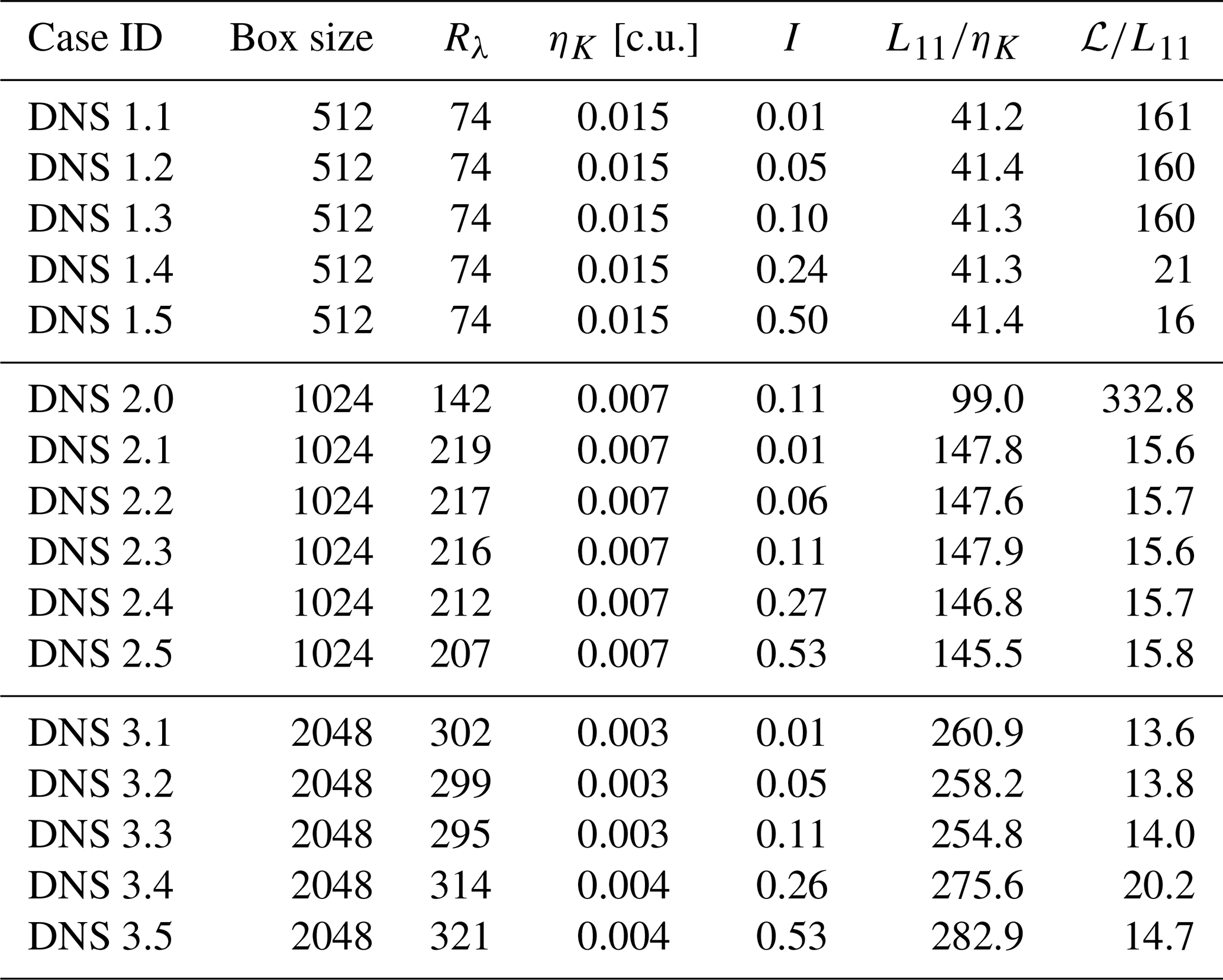
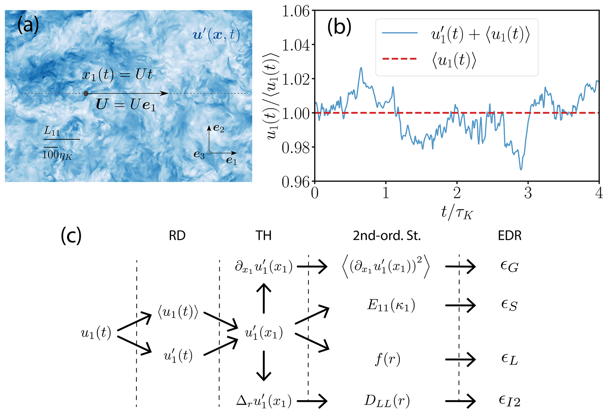
Figure 1 Schematic representation of the procedure for calculating energy dissipation rates from single-point velocity time records. (a) Virtual probe sampling the three-dimensional velocity field of the DNS 3.1 (see Table 2) in time and space at a mean velocity U along its e₁ direction corresponding to a turbulence intensity of 1 %. (b) One-dimensional velocity time series u₁(t) (blue solid) with its corresponding time average U=〈u₁(t)〉 (dashed red line, i.e., Eq. (1)) of the same DNS 3.1, where u₁(t) is re-scaled by 〈u₁(t)〉. (c) Visualization of the workflow from the one-dimensional velocity time record u₁(t) to the energy dissipation rate via different methods. First, u₁(t) is decomposed in its mean and fluctuating part according to Reynolds decomposition (RD). Then, the velocity time series is converted into a one-dimensional velocity field by invoking Taylor's hypothesis (TH). Subsequently, second-order statistics (2nd-ord. St.) of the longitudinal velocity fluctuations, their increments and their first spatial derivative are inferred, from which the energy dissipation rate is estimated with the help of different methods.

2.4 Variable Density Turbulence Tunnel (VDTT)

To evaluate the performance of different methods at Reynolds numbers applicable to atmospheric flows, we use the high-resolution hot-wire measurements of the longitudinal velocity components in the MPIDS VDTT (Bodenschatz et al., 2014). The VDTT datasets used here are associated with $\mathrm{147}\le R_{\mathit{\lambda }}\le \mathrm{5864}$, which enables us to bridge the gap between DNS ($\mathrm{74}\le R_{\mathit{\lambda }}\le \mathrm{321}$) and atmospheric R_λ∼𝒪(10³) (Risius et al., 2015).

The VDTT is a recirculating wind tunnel where the working gas SF₆ is pressurized up to 15 bar to increase its density, thereby enhancing the Taylor-scale Reynolds number. To achieve the same density in air, the pressure would have had to be about 100 bar, which would have required a much thicker tunnel wall and more expensive construction. The VDTT has a horizontal length of 11.68 m and an inner diameter of 1.52 m where the rotation frequency of the fan sets the mean flow velocity ranging from 0.5 to 5.5 m s⁻¹ (Bodenschatz et al., 2014). Long-range correlations of the turbulent flow determine its anisotropy. These long-range correlations are shaped with the help of an active grid consisting of 111 independently rotating winglets (Küchler et al., 2019; Küchler, 2021).

Longitudinal velocity fluctuations are temporally recorded with 30 to 60 µm long nanoscale thermal anemometry probes (NSTAPs; Bailey et al., 2010; Vallikivi et al., 2011, among others) or a 450 µm long conventional hot wire from Dantec (Jørgensen, 2001) corresponding to a resolution of <3η_K and <5η_K, respectively (Küchler et al., 2019), at variable distances from the active grid ranging from ≈ 6–9 m. The velocity measurements have been extensively characterized in terms of the mean flow profiles (Küchler, 2021) as well as the decay of turbulent kinetic energy (Sinhuber et al., 2015; Sinhuber, 2015), exposing velocity probability distribution functions (PDFs) as being flatter than Gaussian (Küchler, 2021). The inertial-range scaling exponent ζ₂ of the longitudinal second-order structure function is in agreement with Kolmogorov's revised phenomenology from 1962 (${\mathit{\zeta }}_{\mathrm{2}}=\mathrm{0.693}\pm \mathrm{0.003}$ for R_λ>2000) for a large variety of wake generation schemes (Küchler et al., 2020). In the case of hot-wire measurements in the VDTT, the ground-truth energy dissipation rate for a given averaging window R is given by the gradient method 〈ϵ_G〉_R, which converges the fastest, as shown in Sect. 3.5.

2.5 Strategies for the evaluation of systematic and random errors

The virtual probes record one-dimensional time records of the DNS longitudinal velocity component, from which the mean energy dissipation rate can be estimated by various methods and compared with the energy dissipation rate obtained directly from the DNS dissipation field. Generally, there are two different errors when estimating the mean energy dissipation rate, namely the systematic errors and random errors. The latter is related to the estimation variance of the mean energy dissipation rate, i.e., the statistical scatter of the 〈ϵ〉_R estimates around the ground truth of the local mean energy dissipation rate defined in Eq. (4). The systematic error in the mean energy dissipation rate estimates expresses itself in a non-vanishing ensemble average of the deviations from the ground truth, i.e., the global volume average defined in Eq. (5).

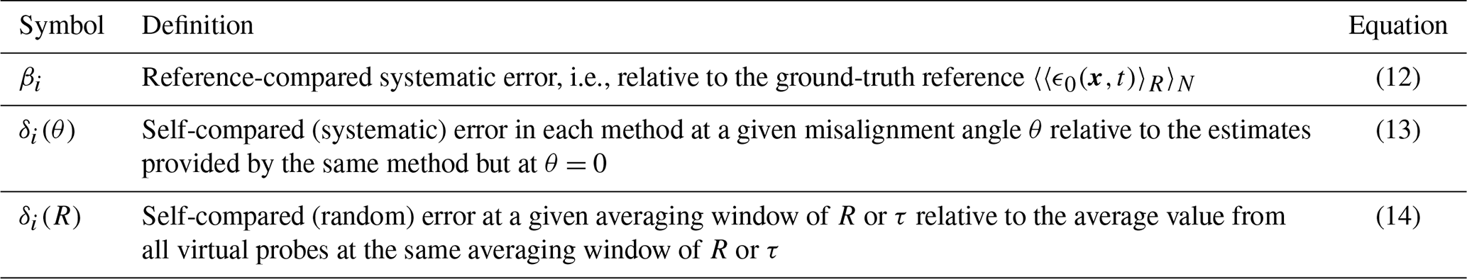
Systematic errors are an inherent feature of the methods used for estimating the dissipation rate but are also affected by experimental limitations and imperfections such as averaging windows and finite turbulence intensity parameterized by R and I, respectively. One way to estimate these errors is to compare the estimated mean energy dissipation rate for a given averaging window R with the ground truth of the DNS defined by the mean energy dissipation rate per virtual probe track, i.e., $\langle {\mathit{ϵ}}_{\mathrm{0}}(\mathit{x},t){\rangle }_{\mathrm{VP},R}$. Another possibility is to compare the estimates with the ensemble average of the mean energy dissipation rate from all virtual probes, i.e., $\langle \langle {\mathit{ϵ}}_{\mathrm{0}}(\mathit{x},t){\rangle }_{\mathrm{VP},R}{\rangle }_N$, where N=1000 is the total number of virtual probes. Either of these possibilities is valid and would be interesting to understand. However, our analysis (not presented here) shows that the second approach is associated with a slightly higher value for the systematic error and a slightly higher standard deviation. For that reason, we have chosen the second approach to make a conservative assessment of the systematic errors; i.e., we compare the estimates of each method against $\langle \langle {\mathit{ϵ}}_{\mathrm{0}}(\mathit{x},t){\rangle }_{\mathrm{VP},R}{\rangle }_N$ by

$$\begin{array}{}\text{(12)}& {\mathit{\beta }}_i={\displaystyle \frac{\langle {\mathit{ϵ}}_i{\rangle }_R}{\langle \langle {\mathit{ϵ}}_{\mathrm{0}}(\mathit{x},t){\rangle }_{\mathrm{VP},R}{\rangle }_N}}-\mathrm{1},\end{array}$$

where $i\in \mathit{\{}G,I\mathrm{3},I\mathrm{2},S,L\mathit{\}}$ and 〈ϵ_i〉_R are the estimates of the energy dissipation rate via method i under the experimental limitation and imperfection such as the size of the averaging window or finite turbulence intensity. To distinguish between the different error terms in this paper, we refer to β as a “reference-compared” systematic error.

In addition, the systematic error can be evaluated by comparing the estimates of the energy dissipation rate obtained by a method with imperfect data against the estimates obtained by the same method with optimal data. We denote these types of errors with δ and refer to them as “self-compared” errors. An experimental imperfection we considered here is the sensor misalignment: this is a non-zero angle of incidence θ between the true longitudinal flow direction along U and the one expected based on the sensor orientation. To investigate the isolated effect of sensor misalignment, we consider a specific set of DNSs with constant turbulence intensity (I=1 %) and the entire track length for each virtual probe. The self-compared systematic error in each method due to misalignment is defined as

$$\begin{array}{}\text{(13)}& {\mathit{\delta }}_i\left(\mathit{\theta }\right)={\displaystyle \frac{{\mathit{ϵ}}_i\left(\mathit{\theta }\right)}{{\mathit{ϵ}}_i\left(\mathrm{0}\right)}}-\mathrm{1},\end{array}$$

where ϵ_i(θ) is the estimate of the energy dissipation rate via method $i\in \mathit{\{}G,I\mathrm{3},I\mathrm{2},S,L\mathit{\}}$ from data with misalignment θ and ϵ_i(0) is the estimated dissipation rate from the same method and flow conditions but with an aligned sensor; i.e., θ=0.

Estimates of the mean energy dissipation rate are susceptible not only to systematic errors, but also to random errors due to statistical uncertainty. For the averaging window, errors given by Eq. (12) would be the best indicator of systematic errors. However, random errors due to the size of the averaging window can also be significant. When the spatial averaging window R (or temporal averaging window τ) is finite, we capture the self-compared random error for each individual method by

$$\begin{array}{}\text{(14)}& {\mathit{\delta }}_i\left(R\right)=\sqrt{{〈{\left({\displaystyle \frac{\langle {\mathit{ϵ}}_i{\rangle }_R}{\langle \langle {\mathit{ϵ}}_i{\rangle }_R{\rangle }_N}}-\mathrm{1}\right)}^{\mathrm{2}}〉}_N},\end{array}$$

where 〈ϵ_i〉_R is the local mean energy dissipation rate based on the averaging window R normalized by its ensemble average, i.e., 〈〈ϵ_i〉_R〉_N. Equation (14) indeed calculates the standard deviation of the normalized 〈ϵ_i〉_R, which is used here as a proxy for the random error. Table 3 provides an overview of the different error types and terminologies used here.

Table 3 Different types of errors investigated in this study and their definitions. Subscript $i\in \mathit{\{}G,I\mathrm{3},I\mathrm{2},S,L\mathit{\}}$, where G stands for the gradient method, I3 for the 4/5 law, I2 for the second-order structure function in the inertial range, S for the spectral method and L for the scaling argument. The averaging window is denoted spatially by R and temporally by τ. The misalignment angle is represented by θ.

3 Results and discussion

In the following, we first focus on the DNS data to calculate ϵ_G, ϵ_I3, ϵ_I2, ϵ_S and ϵ_L from the entire longitudinal velocity time records of all virtual probes and compare these estimates against the ground-truth reference. Then, we systematically investigate the impact of the turbulence intensity, (virtual) probe orientation and averaging window size for all methods of interest. The influence of the flow Reynolds number on the presented results is then discussed by taking into account the VDTT data together with the DNS data. Finally, we provide a proof of concept for a time-dependent dissipation rate calculation by comparing the dissipation time series measured by ϵ_G, ϵ_I2 and ϵ_L and its coarse-grained surrogate. In the following, we use the definitions of systematic and random errors as mentioned in Sect. 2.5 and Table 3.

3.1 Verification of the analytical methods and a first insight into their performance under ideal conditions

To verify the implementation of our methods, only data from cases with a low turbulence intensity of 0.01 and an averaging window covering the entire size of the probe track are used in this section. Furthermore, ϵ_I2 and ϵ_I3 are obtained by a fit according to Eq. (7) with n=2 and n=3, respectively, in the inertial range with $r\in [\mathrm{20}{\mathit{\eta }}_K,\mathrm{500}{\mathit{\eta }}_K]$ for DNS 2.1 and 3.1. Analogously, ϵ_S is inferred from the inertial-range fit in Eq. (9) in the range $f\in [U/(\mathrm{500}{\mathit{\eta }}_K),U/(\mathrm{20}{\mathit{\eta }}_K\left)\right]$. For DNS 1.1 with R_λ=74, due to the absence of an inertial range for low Taylor-scale Reynolds numbers (see Fig. A7), the maximum of Eq. (7) is used to infer ϵ_I2 and ϵ_I3 instead of fitting the inertial range.

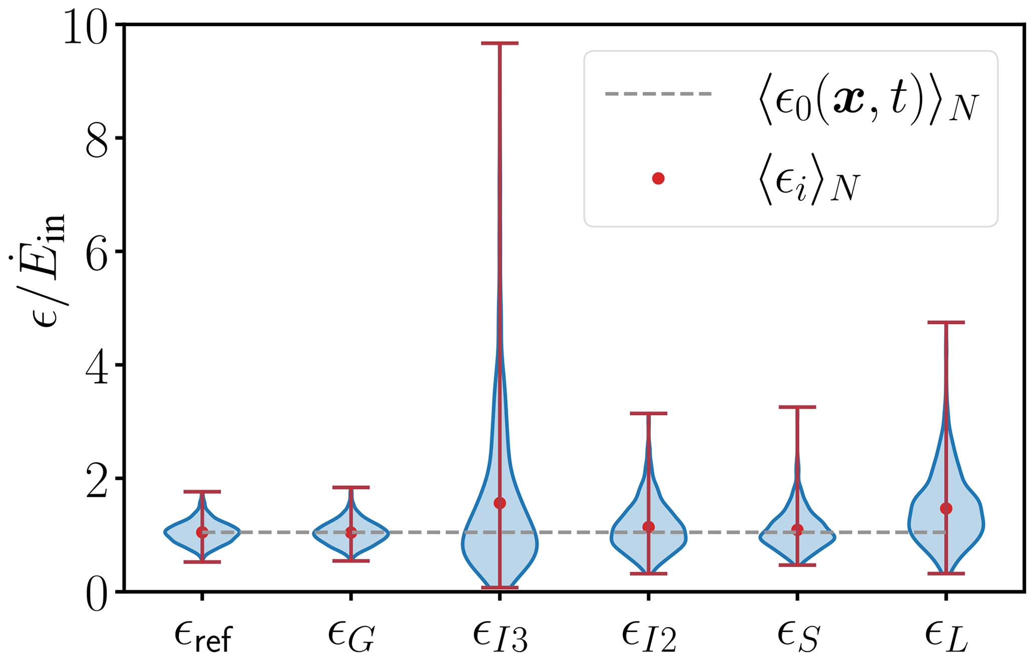
Figure 2 Validation of estimating the energy dissipation rate from ${\mathit{ϵ}}_G,{\mathit{ϵ}}_{I\mathrm{2}},{\mathit{ϵ}}_{I\mathrm{3}},{\mathit{ϵ}}_S$ and ϵ_L re-scaled by the energy injection rate ${\dot{E}}_{\mathrm{in}}$. The data are taken from DNS 3.1 with 1000 probes, R_λ=302, I=1 %, θ=0^∘ and the maximal available averaging window (R≈3550η_K). The ensemble mean of each method 〈ϵ_i〉_N is denoted by red dots where the whiskers extend from the minimal to maximal estimate of ϵ_i where $i\in \mathit{\{}G,I\mathrm{3},I\mathrm{2},S,L\mathit{\}}$. The reference mean energy dissipation rate for each probe is given by ϵ_ref. The dashed line represents the re-scaled global mean energy dissipation rate of DNS 3.1, which is approximated by the ensemble average of the true mean energy dissipation rate along the trajectory of each virtual probe.

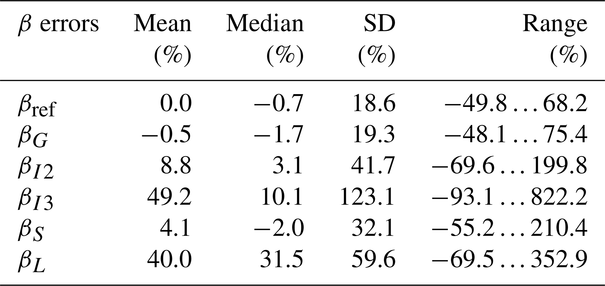
Table 4 Statistics (mean, median, standard deviation (SD) and range) of the reference-compared systematic errors for different methods and case DNS 3.1 with R_λ=302. Here β_ref is defined as $=\langle {\mathit{ϵ}}_{\mathrm{0}}(\mathit{x},t){\rangle }_{\mathrm{VP}}/\langle \langle {\mathit{ϵ}}_{\mathrm{0}}(\mathit{x},t){\rangle }_{\mathrm{VP}}{\rangle }_N-\mathrm{1}$, which shows the actual variability in the dissipation rate field. The last column shows the range of the minimum to maximum percentage deviation from the mean.

The distribution of the mean energy dissipation rate estimated by ${\mathit{ϵ}}_G,{\mathit{ϵ}}_{I\mathrm{2}},{\mathit{ϵ}}_{I\mathrm{3}},{\mathit{ϵ}}_S$ and ϵ_L for each probe at R_λ=302 is shown in Fig. 2 and Table 4. Estimations for other R_λ values are shown in Fig. A1. The best-performing method is the gradient method ϵ_G, with the range also being very close to the range of β_ref, whereas ϵ_I3 is associated with the mean highest deviation. The superior performance of ϵ_G compared with the others is mainly due to the fact that it relies on (dissipation-range) second-order statistics that can be captured with fast statistical convergence within a short sampling interval. Hence, the distributions of ϵ_G and ϵ_ref are similar. ϵ_I3, on the other hand, relies on third-order moments of the velocity increments of inertial scales associated with slower statistical convergence compared to ϵ_G. Therefore, ϵ_I3 requires longer velocity records than ϵ_G to converge under stationary conditions. For this reason, the third-order structure function is not considered further in this study, as one of the main objectives of this study is to evaluate different methods suitable for extracting the time-dependent energy dissipation rate.

Figure 2 and Table 4 also show that the estimates of the energy dissipation rate provided by D_LL(r) and E₁₁(κ₁) are close to each other, which can be explained by the fact that they are both second-order quantities (in real and Fourier space, respectively) connected by f(r). Unlike ϵ_G, both ϵ_I2 and, to a lesser extent, ϵ_S tend to overestimate the energy dissipation rate. However, ϵ_S more strongly depends on properly setting the fit range than ϵ_I2 (Fig. A2). The spectral method ϵ_S can differ by a factor of 2 from ϵ_I2 depending on the high-frequency limit. This factor of 2 is in accordance with a comparison of ϵ_I2 and ϵ_S by a linear fit, resulting in a slope close to 0.5 (Akinlabi et al., 2019). In the DNS, the power spectrum is subject to strong statistical uncertainty at high frequencies without ensemble averaging the spectra of each virtual probe or longer DNS runtimes. As the high-frequency limit of the inertial range of the spectrum is hardly distinguishable from its dissipation range, the choice of the fit range for ϵ_S is related to the fit range of the longitudinal second-order structure function by $f\in \left[U/\left(\mathrm{500}{\mathit{\eta }}_K\right),U/\left(\mathrm{20}{\mathit{\eta }}_K\right)\right]$ as mentioned above. Wacławczyk et al. (2020) found that the estimation of the energy dissipation rate from the power spectral density is generally robust at small wavenumbers (i.e., larger length scales), whereas the second-order structure function performs better at small length scales (i.e., larger wavenumbers). With our choice of the fit range $r\in [\mathrm{20}{\mathit{\eta }}_K,\mathrm{500}{\mathit{\eta }}_K]$ for the DNS 3.1 dataset shown in Fig. 2, we confirm that ϵ_I2 is already reliable at the lower end of the inertial range where dissipative effects are negligible.

Lastly, ϵ_L overestimates by 40 % on average. This systematic overestimation might be due to the difficulty in determining L₁₁, as different methods for estimating the integral length L₁₁ can contribute to the systematic bias in ϵ_L. As mentioned above, we infer the longitudinal integral length from fitting f(r) to the first zero crossing which yields, at least in the DNS of this work, a systematic underestimation due to the scatter in both ${\mathit{\sigma }}_{u_{\mathrm{1}}^{\prime }}$ and L₁₁, as illustrated in Figs. A3 and A4. However, the accuracy of the dissipation constant C_ϵ, which is a function of large-scale forcing and initial conditions (Vassilicos, 2015; Sreenivasan, 1998; Sreenivasan et al., 1995; Burattini et al., 2005), can potentially cause larger mean deviations. Advantageously, the large-scale estimate ϵ_L is applicable to low-resolution measurement. Figure A1 and Table A3 give an overview of the systematic errors in the different methods at different Reynolds numbers, showing that the above conclusions are also valid for lower R_λ.

3.2 The validity of Taylor's hypothesis and the impact of random-sweeping effects

For a large turbulence intensity the local speed and direction of the flow vary significantly in time and space, which hinders the applicability of Taylor's hypothesis. Here, we quantify the impact of random sweeping on the accuracy of determining the mean energy dissipation rate. Therefore, we set the mean speed of the virtual probes in each DNS so that the turbulence intensity, and consequently the random sweeping, is a control parameter.

Figure 3 shows the systematic error β_i for ϵ_G, ϵ_I2, ϵ_S and ϵ_L at different turbulence intensities for DNS 3.1–3.5. For each virtual probe taken into account in Fig. 3, we used the entire time series so that the size of the averaging window is maximal. While each method has a different systematic error and scatter, Fig. 3 indicates that the mean relative deviation of each estimate from the global mean 〈〈ϵ₀(x,t)〉_VP〉_N increases with turbulence intensity. This is particularly strong for the gradient method. For I=1 % and I=10 %, the gradient method has the lowest scatter in terms of the standard deviation ${\mathit{\sigma }}_{{\mathit{\beta }}_G}$ (19.3 % and 27.3 %) and the lowest systematic error in terms of 〈β_G〉_N (−0.5 % and 6.1 %), respectively. At higher turbulence intensities, ϵ_I2 is the least affected method, with 〈β_I2〉_N=6.5 % and ${\mathit{\sigma }}_{{\mathit{\beta }}_{I\mathrm{2}}}=\mathrm{37.2}$ % for I=25 % as well as 〈β_I2〉_N=24.5 % and ${\mathit{\sigma }}_{{\mathit{\beta }}_{I\mathrm{2}}}=\mathrm{56.9}$ % for I=50 %. At the highest turbulence intensities, both ϵ_L and ϵ_S are associated with lower mean β than that of ϵ_G.

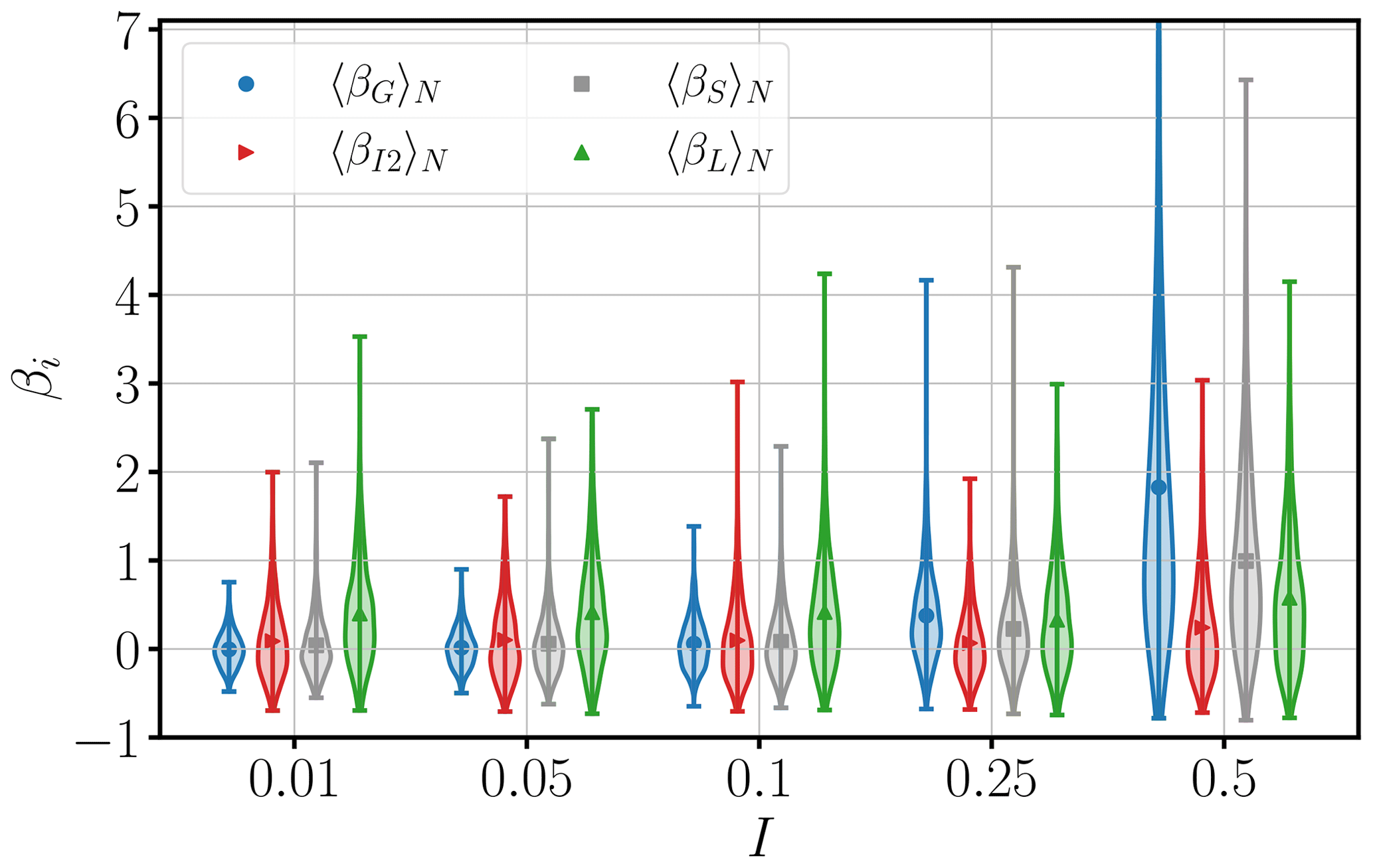
Figure 3 Systematic error β_i in Eq. (12) as a function of turbulence intensity $I\in \mathit{\{}\mathrm{0.01},\mathrm{0.05},\mathrm{0.1},\mathrm{0.25},\mathrm{0.5}\mathit{\}}$ for ϵ_G (•), ϵ_I2 (▸), ϵ_S (▪) and ϵ_L (▴). The energy dissipation rates are estimated from each longitudinal velocity time series of DNS 3.1–3.5 with ideal alignment (θ=0^∘) where the maximal available window size was used. The fit range for the inertial range of the power spectral density is chosen to be within $U/\left(\mathrm{500}{\mathit{\eta }}_K\right)\le f\le U/\left(\mathrm{20}{\mathit{\eta }}_K\right)$, where η_K is the Kolmogorov length scale, and, equivalently in the space domain, $\mathrm{20}{\mathit{\eta }}_K\le r\le \mathrm{500}{\mathit{\eta }}_K$ for the longitudinal second-order structure function. The upper limit of the y axis is chosen to be 7.1 in order to improve the plot visibility (upper whiskers of ϵ_G for I=50 % are not shown for better visibility of other cases).

The fraction of track samples that can lead to a deviation of larger than 100 % increases from 0 % to ∼60 % for ϵ_G as the turbulence intensity increases from 1 % to 50 %. We hypothesize that these deviations of the mean are the result of random-sweeping effects, which limit the applicability of Taylor's hypothesis. In frequency space, Taylor's hypothesis (Taylor, 1938) establishes a one-to-one mapping between the frequency and the streamwise wavenumber; i.e., ω=κ₁U. As the turbulence intensity grows, a randomly sweeping mean velocity smears out this correspondence between frequencies and wavenumbers. For the spectrum, this smearing out effectively moves energy from larger scales to smaller and less energetic ones (Lumley, 1965; Tennekes, 1975). Therefore, it leads to an overestimation in the inertial and dissipation range of the spectrum, thus affecting the inertial range and gradient method. To visualize this overestimation, we evaluate the effect of random sweeping on the spectrum (Eq. B2) numerically for different turbulence intensities at the example of a model spectrum (Eq. B4). The result is shown in Fig. 4, where the spectrum is premultiplied by ${\mathit{\kappa }}_{\mathrm{1}}^{\mathrm{2}}$ to later highlight the effect on the gradient method. Here, the overestimation is most pronounced in the dissipative range.

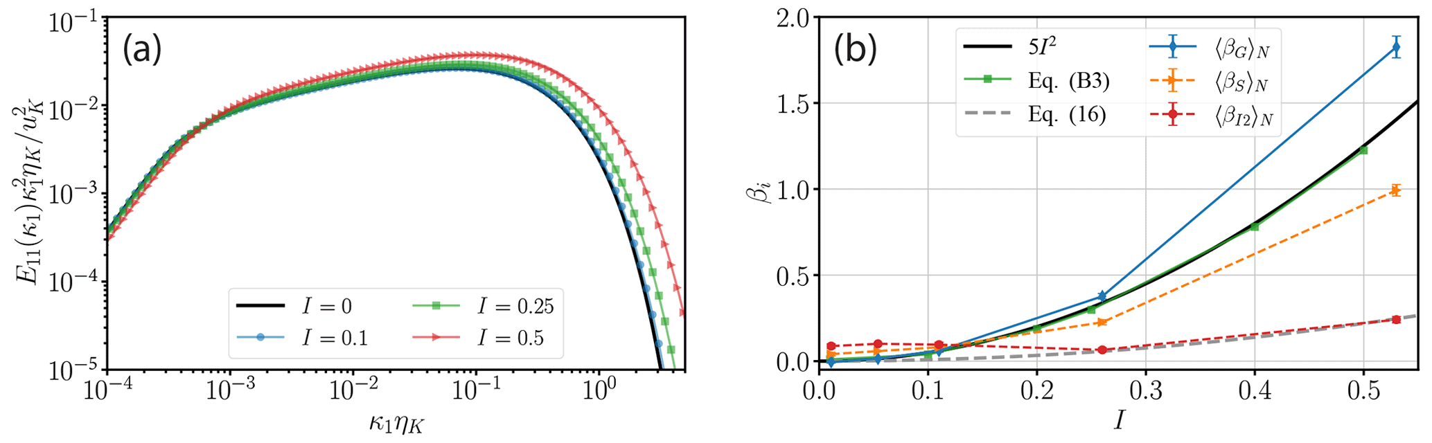
Figure 4 The effects of random sweeping on the energy dissipation estimates. (a) Premultiplied model energy spectrum with random-sweeping effects in Eq. (B2) for turbulence intensities $I\in \mathit{\{}\mathrm{0.1},\mathrm{0.25},\mathrm{0.5}\mathit{\}}$, where the original energy spectrum corresponds to I=0. $u_K=(\mathit{\nu }\langle \mathit{ϵ}\rangle {)}^{\mathrm{1}/\mathrm{4}}$ is the Kolmogorov velocity scale. (b) Systematic overprediction illustrated by the relative error β_i in Eq. (12) at different turbulence intensities. The systematic overprediction by Lumley (1965) (solid black) matches the numerically obtained systematic error β_G for the gradient method relative to the ground-truth reference 〈ϵ〉 by using the model spectrum and numerically evaluating the integral in Eq. (B3) (green squares). Both estimate the data obtained from DNS 3.1–3.5 (blue diamonds) up to a turbulence intensity of I=25 % reasonably well. Moreover, we show the systematic overprediction of inertial-sub-range methods (β_S: orange triangles and β_I2: red circles, both from Eq. 12) compared with the analytically derived error obtained by the random-sweeping model (β_I2,S, Eq. 16, grey dashed).

To quantify the impact of random sweeping on estimates of 〈ϵ〉, we first consider the influence of random sweeping on the gradient method. For the gradient method, Lumley (1965) and Wyngaard and Clifford (1977) have shown that in isotropic turbulence, random sweeping leads to an relative deviation of the volume-averaged mean energy dissipation rate by

$$\begin{array}{}\text{(15)}& \begin{array}{rl}& {\displaystyle \frac{{\mathit{ϵ}}_G}{\langle \mathit{ϵ}\rangle }}-\mathrm{1}={\mathit{\beta }}_G=\mathrm{5}{I}^{\mathrm{2}}\text{with}\\ & {\mathit{ϵ}}_G=\mathrm{15}\mathit{\nu }\int {\mathit{\kappa }}_{\mathrm{1}}^{\mathrm{2}}{E}_{\mathrm{11}}\left({\mathit{\kappa }}_{\mathrm{1}}\right)d{\mathit{\kappa }}_{\mathrm{1}}=\langle \mathit{ϵ}\rangle \left[\mathrm{1}+\mathrm{5}{I}^{\mathrm{2}}\right].\end{array}\end{array}$$

We illustrate this result in Appendix B, where we consider a model wave-number–frequency spectrum (Wilczek and Narita, 2012; Wilczek et al., 2014), which is based on the same modeling assumptions used in Wyngaard and Clifford (1977). Due to the ${\mathit{\kappa }}_{\mathrm{1}}^{\mathrm{2}}$ weighting of the gradient method, the mean dissipation rate estimate is highly sensitive to the viscous cutoff of the energy spectrum, which is overestimated by random-sweeping effects (see Fig. 4). As a consequence, deviations in the estimated dissipation rate grow rapidly with turbulence intensity. In the right panel of Fig. 4, we compare the effect of random sweeping on the gradient method obtained with a model spectrum, the one computed by Lumley (1965) and the observed deviations by measurements of the virtual probes in a DNS flow; shown here are the DNS 3.1–3.5 cases. In fact, the estimate from Lumley (1965) can explain the magnitude of deviations observed by the virtual probes in the case of ϵ_G up to I=25 %. The strong deviation in β_G at I=50 % is likely due to the sensitivity of the gradients to the space-to-time conversion via Taylor's hypothesis: at high turbulence intensities, the mean velocity becomes smaller compared with the fluctuations. Therefore, the error in estimating the mean velocity due to the finite averaging window (Eq. 2) increases relative to the mean velocity. Larger relative errors in the estimated mean velocity lead – applying Taylor's hypothesis – to both under- and overestimated spatial gradients for the individual averaging windows, in addition to the effect of random sweeping. Similarly this results in an additional overestimation of the dissipation rate. These deviations do not appear in evaluating random-sweeping effects based on a model spectrum, as there the mean velocity is a parameter we choose.

Now let us consider the two inertial-sub-range methods. Here, as one can see in Figs. 3 and 4, the increase in the mean relative deviation, β_i, is less pronounced. In the inertial sub-range, random sweeping causes an overestimation of the spectrum of merely several percent, while the inertial-range scaling is preserved as shown in Wyngaard and Clifford (1977) and Wilczek et al. (2014). As both the second-order structure function and the spectral method are based on the inertial sub-range of the energy spectrum, the effect of a randomly sweeping mean velocity on ϵ_I2 and ϵ_S is expected to be small. Here, the overestimation of the spectrum can be used to express the relative systematic deviation in both ϵ_I2 and ϵ_S for different turbulence intensities analytically:

$$\begin{array}{}\text{(16)}& \begin{array}{rl}& {\displaystyle \frac{{\mathit{ϵ}}_{I\mathrm{2}/S}}{\langle \mathit{ϵ}\rangle }}-\mathrm{1}={\mathit{\beta }}_{I\mathrm{2}/S}={\left(C_{\mathrm{T}}\left(I\right)\right)}^{\mathrm{3}/\mathrm{2}}-\mathrm{1}\text{with}\\ & C_{\mathrm{T}}\left(I\right)={\displaystyle \frac{\mathrm{5}}{\mathrm{6}}}\underset{\mathrm{0}}{\overset{\mathrm{\infty }}{\int }}\left[\text{erf}\left({\displaystyle \frac{y+\mathrm{1}}{\sqrt{\mathrm{2}}I}}\right)-\text{erf}\left({\displaystyle \frac{y-\mathrm{1}}{\sqrt{\mathrm{2}}I}}\right)\right]y^{\mathrm{2}/\mathrm{3}}\mathrm{d}y,\end{array}\end{array}$$

where C_T(I) quantifies the spectral overestimation as a function of mean wind and fluctuations defined as in Wilczek et al. (2014). In Fig. 4b, we compare the observed deviations from the DNS to Eq. (16). This shows that Eq. (16) underestimates β_I2 for $I\in \mathit{\{}\mathrm{0.01},\mathrm{0.05},\mathrm{0.1}\mathit{\}}$ (i.e., DNS 3.1, 3.2 and 3.3). The underestimation is most likely due to additional random errors associated with finite averaging window lengths. It is obvious from Table 2 that DNS 3.3 statistically has the shortest probe tracks of ∼3440η_K (DNS 3.1: ∼3550η_K, DNS 3.2: ∼3560η_K). Nonetheless, β_I2 matches the prediction of Eq. (16) for $I\in \mathit{\{}\mathrm{0.25},\mathrm{0.5}\mathit{\}}$ where the corresponding probe tracks statistically amount to ∼5570η_K and ∼4260η_K, respectively. The effect of the averaging window size on ϵ_I2 is explored in Sect. 3.4. We conclude that Eq. (16) can be used to estimate the error introduced by random sweeping of ϵ_I2.

For the spectral method, Eq. (16) underestimates the relative error β_S for all turbulence intensities. This may be due to the strong dependence of ϵ_S on the U-based fitting range (see Fig. A2), i.e., $f\in \left[U/\left(\mathrm{500}{\mathit{\eta }}_K\right),U/\left(\mathrm{20}{\mathit{\eta }}_K\right)\right]$, which can differ significantly between virtual probes at high turbulence intensities. Further work is needed to assess the dependence of the spectral method on the choice of the fit range for finite turbulence intensities.

Overall, random-sweeping effects explain why the gradient method is more sensitive to turbulence intensity than inertial-range methods. Here, random sweeping accurately captures the deviations of the second-order structure function method as a function of turbulence intensity, whereas it can only partially account for the observed deviations for the spectral method.

3.3 Probe misalignment

In this section, we assess the influence of probe misalignment with respect to the mean flow direction on estimating the energy dissipation rate at the energy injection scale, the inertial range and the dissipation range. Here, we assume the angle θ between the (virtual) anemometer and the global mean wind direction $\frac{\mathit{U}}{\left|\mathit{U}\right|}$ to be constant throughout the sampling trajectory. As can be seen from Eq. (C6), ϵ_L depends on θ. Then, the analytically derived error for ϵ_L due to misalignment of the sensor and the longitudinal wind direction is given by

$$\begin{array}{}\text{(17)}& {\mathit{\delta }}_L\left(\mathit{\theta }\right)={\displaystyle \frac{{\mathit{ϵ}}_L\left(\mathit{\theta }\right)}{{\mathit{ϵ}}_L\left(\mathrm{0}\right)}}-\mathrm{1}={\displaystyle \frac{\mathrm{2}}{\cos \mathit{\theta }(\mathrm{1}+{\cos }^{\mathrm{2}}\mathit{\theta })}}-\mathrm{1},\end{array}$$

where ϵ_L(θ) represents the energy dissipation that is derived given an angle of incidence θ, and ϵ_L(0) is the reference value for perfect alignment of the mean flow direction and the probe, i.e., when θ=0.

Analogously, the second-order structure function tensor is affected by misalignment (cf. Appendix C). Thus, it can be shown that the analytically derived error δ_I2(θ) as a function of θ reads

$$\begin{array}{}\text{(18)}& {\mathit{\delta }}_{I\mathrm{2}}\left(\mathit{\theta }\right)={\displaystyle \frac{{\mathit{ϵ}}_{I\mathrm{2}}\left(\mathit{\theta }\right)}{{\mathit{ϵ}}_{I\mathrm{2}}\left(\mathrm{0}\right)}}-\mathrm{1}={\left({\displaystyle \frac{\mathrm{4}-{\cos }^{\mathrm{2}}\mathit{\theta }}{\mathrm{3}}}\right)}^{\mathrm{3}/\mathrm{2}}{\displaystyle \frac{\mathrm{1}}{\cos \mathit{\theta }}}-\mathrm{1},\end{array}$$

where ϵ_I2(θ) represents the energy dissipation that is derived given an angle of incidence θ, and ϵ_I2(0) is the reference value for perfect alignment of the mean flow direction and the probe. As outlined in Appendix C and with Eq. (5), the analytically derived error in ϵ_G as a function of θ can be calculated to

$$\begin{array}{}\text{(19)}& {\mathit{\delta }}_G\left(\mathit{\theta }\right)={\displaystyle \frac{{\mathit{ϵ}}_G\left(\mathit{\theta }\right)}{{\mathit{ϵ}}_G\left(\mathrm{0}\right)}}-\mathrm{1}=\mathrm{2}\left({\displaystyle \frac{\mathrm{1}}{{\cos }^{\mathrm{2}}\mathit{\theta }}}-\mathrm{1}\right),\end{array}$$

where ϵ_G(θ) represents the energy dissipation that is derived given an angle of incidence θ, and ϵ_G(0) is the reference value for perfect alignment of the mean flow direction and the probe.

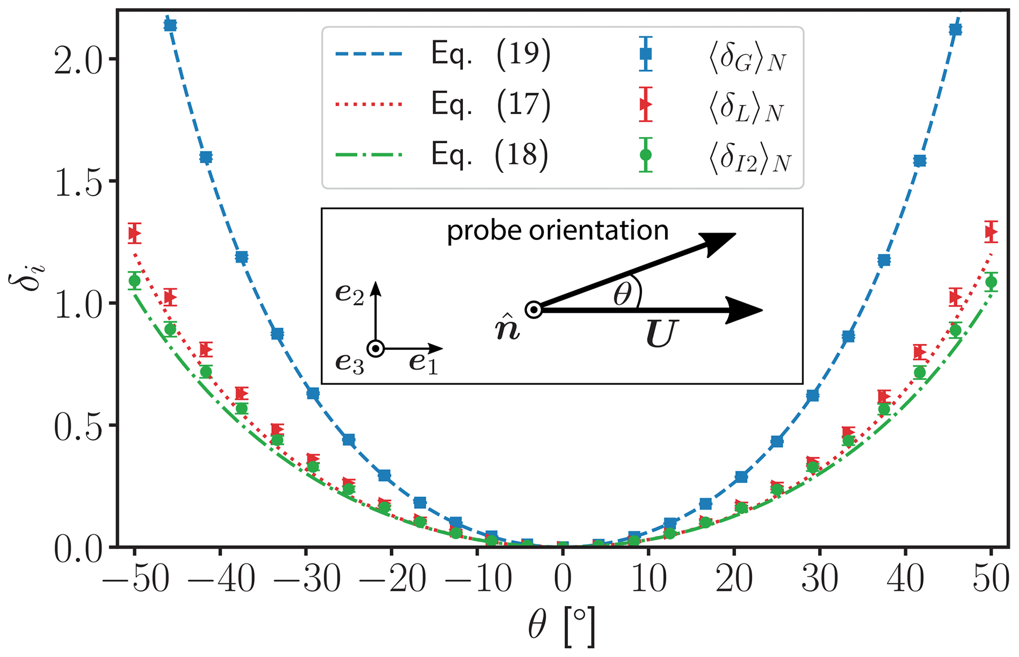
Figure 5 Influence of misalignment between probe orientation and the mean flow direction U in terms of the average error in the energy dissipation rate δ_i(θ) as a function of the angle of attack θ. The energy dissipation rates are derived from DNS 3.1 with a turbulence intensity of 1 %, an R_λ=293 and the maximally available window size. The error bars are given by the standard error of the mean. The analytically derived errors δ_L(θ), δ_I2(θ) and δ_G(θ) are given by Eqs. (17), (18) and (19), respectively. The ordinate is limited from 0 to 2.2 to guarantee better visibility for δ_L(θ) and δ_I2(θ). The inset visualizes the misalignment angle θ between the probe orientation and the mean flow direction U. The rotation axis is denoted by $\widehat{\mathit{n}}$. As mentioned above, the mean flow direction U is considered to be the longitudinal direction of the flow.

To compare the analytical expressions with DNS results, the sensing orientation of the virtual probes is rotated around the e₃ axis in the coordinate system of each virtual probe by an angle θ relative to their direction of motion, i.e., the e₁ axis. Then, ϵ_L(θ), ϵ_I2(θ) and ϵ_G(θ) are inferred from the new longitudinal velocity component. The ensemble-averaged relative errors in the estimated energy dissipation rates δ(θ) due to misalignment are shown as a function of θ in Fig. 5 in the range of ±50^∘ both for DNS and for the analytically derived Eqs. (17)–(19). In general, the ensemble-averaged systematic errors follow the analytically derived errors reliably in terms of the limits of accuracy for all R_λ values at turbulence intensity I=1 %. The longitudinal second-order structure function is the best-performing method, with a systematic error 〈δ_I2〉_N of lower than 20 % for $\mathit{\theta }\in [-\mathrm{25}{}^{\circ },\mathrm{25}{}^{\circ }]$, which increases to 100 % at $\mathit{\theta }=\pm \mathrm{50}$^∘. 〈δ_L〉_N is similarly affected by misalignment but is slightly larger than 〈δ_I2〉_N. Despite its rapid statistical convergence, ϵ_G is the method most vulnerable to misalignment compared with the other two methods.

In experiments where the sensor can be aligned to the mean wind direction within $\mathit{\theta }\in [-\mathrm{10}{}^{\circ },\mathrm{10}{}^{\circ }]$ over the entire record time, δ_i(θ) is expected to be small. Further work is needed to evaluate the impact of a time-dependent misalignment angle θ(t). We suppose that keeping the angle of attack θ fixed over the entire averaging window, here the entire time record of each probe, potentially leads to overestimation of δ_i(θ), with θ being a function of time in practice.

3.4 Systematic errors due to the finite averaging window of size R

Here, our goal is to investigate how the accuracy of estimating the global mean energy dissipation rate depends on the averaging window size by investigating the associated systematic and random errors individually. To do this, we select an averaging window of size R from the beginning of each track of virtual probes for the DNS 3.1 case. In this way, we obtain one subrecord for each virtual probe, which amounts to a total of 1000 subrecords for each averaging window R. From each of these subrecords, mean values of ϵ₀ (i.e., $\langle {\mathit{ϵ}}_{\mathrm{0}}(\mathit{x},t){\rangle }_{\mathrm{VP},R}$), 〈ϵ_G〉_R, 〈ϵ_L〉_R and 〈ϵ_I2〉_R are then evaluated. The smallest R considered for these analyses is 501η_K, which is limited by the upper bound of the fitting range $r\in [\mathrm{20}{\mathit{\eta }}_K,\mathrm{500}{\mathit{\eta }}_K]$ for estimating ϵ_I2. The largest window size considered in this section is 3000η_K, which is limited by the total length of the virtual probe track (Table 2).

Before comparing estimates of the energy dissipation rate using different methods, let us first compare the locally averaged energy dissipation rate $\langle {\mathit{ϵ}}_{\mathrm{0}}(\mathit{x},t){\rangle }_{\mathrm{VP},R}$ with the instantaneous energy dissipation rate, which is shown in Fig. 6a. All averaging window sizes create PDFs with similar shapes but significantly different from the shape of the instantaneous field. The larger the volume over which the dissipation field is averaged, the more the PDF$(\langle {\mathit{ϵ}}_{\mathrm{0}}(\mathit{x},t\left){\rangle }_{\mathrm{VP},R}\right)$ converges to a peak at the global mean energy dissipation rate normalized by ${\dot{E}}_{\mathrm{in}}$, i.e., $\langle {\mathit{ϵ}}_{\mathrm{0}}(\mathit{x},t)\rangle /{\dot{E}}_{\mathrm{in}}\approx \mathrm{1.0}$.

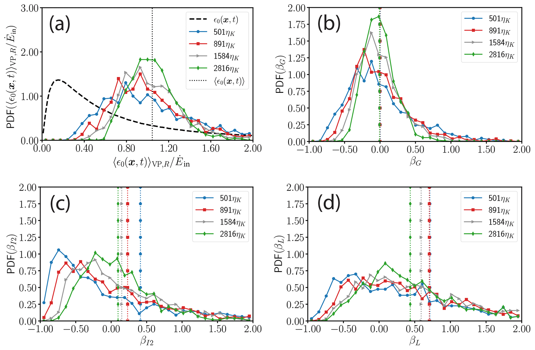
Figure 6 The effect of the averaging window size R (a) on the distribution of $\langle {\mathit{ϵ}}_{\mathrm{0}}(\mathit{x},t){\rangle }_{\mathrm{VP},R}/{\dot{E}}_{\mathrm{in}}$ and on the accuracy of estimates obtained via (b) 〈ϵ_G〉_R, (c) 〈ϵ_I2〉_R and (d) 〈ϵ_L〉_R in terms of the systematic errors β_G, β_I2 and β_L, respectively, from the ground-truth reference $\langle {\mathit{ϵ}}_{\mathrm{0}}(\mathit{x},t){\rangle }_{\mathrm{VP},R}$ as given by Eq. (12). The velocity time records of the longitudinal component are taken from DNS 3.1 (R_λ=302, I=1 %, θ=0^∘). In panel (a), the distribution of the instantaneous dissipation rate ${\mathit{ϵ}}_{\mathrm{0}}(\mathit{x},t)/{\dot{E}}_{\mathrm{in}}$ sampled by all virtual probes is shown by the dashed line, and the global average energy dissipation rate normalized by ${\dot{E}}_{\mathrm{in}}$ is shown by the vertical dotted line. The other PDFs in (a) are from the local average of the energy dissipation rate obtained from a window of size R at the beginning of each virtual probe, i.e., 1000 averaged values for a given R. In panels (b), (c) and (d) the vertical dotted lines correspond to the ensemble averages of the systematic errors β_i. The ensemble average of β_G decreases slightly from 0.4 % for R=501η_K to −0.7 % for R=2815η_K where the standard deviation of β_G decreases from 50 % to 22 %. The ensemble average of β_I2 decreases from 41 % to 10 % and the standard deviation from 185 % to 5 %. β_L exhibits stronger deviations (mean β_L of ∼44 % and standard deviation of ∼67 % for R=2816η_K).

We can further explore the influence of the averaging window R for each method by examining the distribution of systematic errors, i.e., β_i, as shown in Fig. 6b–d. The first main point to note is the fact that at small R all methods tend to peak at a dissipation rate lower than the global. Hence, the mean energy dissipation rate is most likely underestimated. All PDF(β_i(R)) values become narrower, and the mean relative error β_i(R) converges to zero as R increases. The second main point to consider is the statistical uncertainty, causing a random error in estimating the local mean energy dissipation rate $\langle {\mathit{ϵ}}_{\mathrm{0}}(\mathit{x},t){\rangle }_{\mathrm{VP},R}$. As can be seen in Fig. 6b–d, the width of the distribution is wide with asymmetric long tails, especially for β_I2 and β_L. This is an indication that high random errors are to be expected in the estimation of the mean energy distribution rate.

3.5 Random errors due to the finite averaging window of size R

We now analytically focus on random errors associated with ϵ_G, ϵ_L and ϵ_I2. We denote 〈ϵ_G〉_R, 〈ϵ_L〉_R and 〈ϵ_I2〉_R as the energy dissipation rates that are estimated for a longitudinal velocity time record for a window of size R. For the calculation of random errors caused by the choice of the size of the averaging window, we consider DNS 1.3, 2.3 and 3.3, as well as wind tunnel experiments that all have a comparable turbulence intensity of I≈10 %.

Both the second-order structure function in Eq. (A3) and the scaling argument in Eq. (10) depend on the variance $\langle u_{\mathrm{1}}^{\prime \mathrm{2}}\rangle$ of the longitudinal velocity time record. ϵ_G is also related to $\langle u_{\mathrm{1}}^{\prime \mathrm{2}}\rangle$ through Eqs. (6) and (A1). The variance $\langle u_{\mathrm{1}}^{\prime \mathrm{2}}\rangle$ itself is subject to both systematic and random errors in the case of a finite averaging window R<∞. Assuming an ergodic and hence stationary velocity fluctuation time record with a vanishing mean, the systematic error in estimating the variance over an averaging window of size R is given by (following Lenschow et al., 1994, while applying Taylor's hypothesis)

$$\begin{array}{}\text{(20)}& {\mathrm{\Delta }}_{\langle u_{\mathrm{1}}^{\prime \mathrm{2}}\rangle }={〈{\displaystyle \frac{\langle u_{\mathrm{1}}^{\prime \mathrm{2}}{\rangle }_R}{\langle u_{\mathrm{1}}^{\prime \mathrm{2}}\rangle }}-\mathrm{1}〉}_N\approx -\mathrm{2}{\displaystyle \frac{L_{\mathrm{11}}}{R}},\end{array}$$

where $\langle u_{\mathrm{1}}^{\prime \mathrm{2}}{\rangle }_R$ is the estimated variance based on the (finite) averaging window R, $\langle u_{\mathrm{1}}^{\prime \mathrm{2}}\rangle$ is the true variance and it is assumed R≫L₁₁. The always negative error predicted by Eq. (20) indicates that, for finite averaging window sizes, the variance $\langle u_{\mathrm{1}}^{\prime \mathrm{2}}\rangle$ is always statistically underestimated, which agrees with Fig. A3a. Equation (20) furthermore indicates that the systematic error in the variance estimates can be neglected for sufficiently long averaging windows R≫L₁₁.

The variance estimates are also subject to statistical uncertainty, which is also known as the random error in variance estimation (Lenschow et al., 1994). Assuming that $u_{\mathrm{1}}^{\prime }\left(t\right)$, which has a zero mean, can be modeled by a stationary Gaussian process and that its autocorrelation function is sufficiently well represented by an exponential, the random error in estimating the variance can be expressed as (following Lenschow et al., 1994, while applying Taylor's hypothesis)

$$\begin{array}{}\text{(21)}& \begin{array}{rl}{e}_{\mathrm{rand}}& =\sqrt{{〈{\left({\displaystyle \frac{\langle u_{\mathrm{1}}^{\prime \mathrm{2}}{\rangle }_R-{〈\langle u_{\mathrm{1}}^{\prime \mathrm{2}}{\rangle }_R〉}_N}{\langle u_{\mathrm{1}}^{\prime \mathrm{2}}\rangle }}\right)}^{\mathrm{2}}〉}_N}\\ & \approx \sqrt{{〈{\left({\displaystyle \frac{\langle u_{\mathrm{1}}^{\prime \mathrm{2}}{\rangle }_R}{{〈\langle u_{\mathrm{1}}^{\prime \mathrm{2}}{\rangle }_R〉}_N}}-\mathrm{1}\right)}^{\mathrm{2}}〉}_N}\approx \sqrt{{\displaystyle \frac{\mathrm{2}{L}_{\mathrm{11}}}{R}}},\end{array}\end{array}$$

where it is assumed R≫L₁₁ such that the systematic error can be neglected and, hence, ${〈\langle u_{\mathrm{1}}^{\prime \mathrm{2}}{\rangle }_R〉}_N\approx \langle u_{\mathrm{1}}^{\prime \mathrm{2}}\rangle$. Here, ${〈\langle u_{\mathrm{1}}^{\prime \mathrm{2}}{\rangle }_R〉}_N$ is the ensemble average of the variance estimates $\langle u_{\mathrm{1}}^{\prime \mathrm{2}}{\rangle }_R$ for an averaging window R. It can be seen that e_rand is larger than the systematic error in Eq. (20) when R>L₁₁.

Consequently, the estimation of the mean energy dissipation rate by the scaling argument in Eq. (10) is affected by the (absolute) random error in the variance estimation given by the product of e_rand and ${〈\langle u_{\mathrm{1}}^{\prime \mathrm{2}}{\rangle }_R〉}_N$. Invoking the Gaussian error propagation, the analytically estimated error reads

$$\begin{array}{}\text{(22)}& \begin{array}{rl}& {\mathit{\delta }}_L\left(R\right)\\ & ={\displaystyle \frac{\mathrm{1}}{\langle {\mathit{ϵ}}_L{\rangle }_R}}{\displaystyle \frac{\partial \langle {\mathit{ϵ}}_L{\rangle }_R}{\partial \langle u_{\mathrm{1}}^{\prime \mathrm{2}}{\rangle }_R}}\underset{\mathrm{absolute}\mathrm{random}\mathrm{error}\mathrm{in}\langle u_{\mathrm{1}}^{\prime \mathrm{2}}{\rangle }_R}{\underbrace{\underset{\mathrm{relative}\mathrm{random}\mathrm{error}\mathrm{in}\langle u_{\mathrm{1}}^{\prime \mathrm{2}}{\rangle }_R}{\underbrace{e_{\mathrm{rand}}}}{〈\langle u_{\mathrm{1}}^{\prime \mathrm{2}}{\rangle }_R〉}_N}}\\ & \approx {\displaystyle \frac{\mathrm{3}}{\mathrm{2}}}\sqrt{{\displaystyle \frac{\mathrm{2}{L}_{\mathrm{11}}}{R}}},\end{array}\end{array}$$

where e_rand is the relative random error in the variance estimate of the velocity fluctuations $\langle u_{\mathrm{1}}^{\prime \mathrm{2}}{\rangle }_R$ defined in Eq. (21), and $\langle u_{\mathrm{1}}^{\prime \mathrm{2}}{\rangle }_R$ is the variance estimate of $u_{\mathrm{1}}^{\prime }$ based on the averaging window R. Then, the absolute random error in the variance estimate of the velocity fluctuations $\langle u_{\mathrm{1}}^{\prime \mathrm{2}}{\rangle }_R$ is given by $e_{\mathrm{rand}}\langle u_{\mathrm{1}}^{\prime \mathrm{2}}{\rangle }_R$. δ_L(R) is a relative error itself, hence the prefactor $\mathrm{1}/\langle {\mathit{ϵ}}_L{\rangle }_R$. Notably, δ_L(R) scales as $R^{-\mathrm{1}/\mathrm{2}}$.

Similarly, the longitudinal second-order structure function is also affected by the estimation variance $\langle {u_{\mathrm{1}}^{\prime }}^{\mathrm{2}}{\rangle }_R$,

$$\begin{array}{}\text{(23)}& \begin{array}{rl}{e}_{D_{\mathrm{LL}}}& =\sqrt{{〈{\left({\displaystyle \frac{D_{\mathrm{LL}}(r;R)}{\langle D_{\mathrm{LL}}(r;R){\rangle }_N}}-\mathrm{1}\right)}^{\mathrm{2}}〉}_N}\\ & =\sqrt{{〈{\left({\displaystyle \frac{\mathrm{2}\langle u_{\mathrm{1}}^{\prime \mathrm{2}}{\rangle }_R\left(\mathrm{1}-f\left(r\right)\right)}{\mathrm{2}{〈\langle u_{\mathrm{1}}^{\prime \mathrm{2}}{\rangle }_R〉}_N\left(\mathrm{1}-f\left(r\right)\right)}}-\mathrm{1}\right)}^{\mathrm{2}}〉}_N}\\ & \approx \sqrt{{\displaystyle \frac{\mathrm{2}{L}_{\mathrm{11}}}{R}}},\end{array}\end{array}$$

where D_LL(r;R) is the longitudinal second-order structure function evaluated over an averaging window of size R and under the assumption that the longitudinal autocorrelation function f(r) is sufficiently converged over the range of the averaging window. This is a simplistic assumption that may be questionable in some cases, but a more robust evaluation of the validity of the assumption is complex and beyond the scope of this study.

Thus, the uncertainty in estimating the variance propagates to 〈ϵ_I2〉_R relying on D_LL(r;R) (Eq. 7 for n=2). The random error δ_I2(R) can be analytically inferred from the random error in the second-order structure function ${\mathit{\sigma }}_{D_{\mathrm{LL}}}$ by Gaussian error propagation, yielding

$$\begin{array}{}\text{(24)}& {\mathit{\delta }}_{I\mathrm{2}}\left(R\right)={\displaystyle \frac{\mathrm{1}}{\langle {\mathit{ϵ}}_{I\mathrm{2}}{\rangle }_R}}{\displaystyle \frac{\partial \langle {\mathit{ϵ}}_{I\mathrm{2}}{\rangle }_R}{\partial D_{\mathrm{LL}}}}{e}_{D_{\mathrm{LL}}}\langle D_{\mathrm{LL}}(r;R){\rangle }_N\approx {\displaystyle \frac{\mathrm{3}}{\mathrm{2}}}\sqrt{{\displaystyle \frac{\mathrm{2}{L}_{\mathrm{11}}}{R}}},\end{array}$$

which shows that δ_I2(R) scales as $R^{-\mathrm{1}/\mathrm{2}}$ similar to δ_L(R). Considering Eqs. (6) and (A1), the gradient method can also be expressed as a function of the variance $\langle u_{\mathrm{1}}^{\prime \mathrm{2}}\rangle$. Hence, Gaussian error propagation yields

$$\begin{array}{}\text{(25)}& \begin{array}{rl}{\mathit{\delta }}_G\left(R\right)& ={\displaystyle \frac{\mathrm{1}}{\langle {\mathit{ϵ}}_G{\rangle }_R}}{\displaystyle \frac{\partial \langle {\mathit{ϵ}}_G{\rangle }_R}{\partial \langle u_{\mathrm{1}}^{\prime \mathrm{2}}{\rangle }_R}}{e}_{\mathrm{rand}}{〈\langle u_{\mathrm{1}}^{\prime \mathrm{2}}{\rangle }_R〉}_N\\ & =-\mathrm{15}\mathit{\nu }{\displaystyle \frac{\mathrm{1}}{\langle {\mathit{ϵ}}_G{\rangle }_R}}\underset{\left|\mathit{r}\right|\to \mathrm{0}}{lim}{\partial }_r^{\mathrm{2}}f\left(r\right)e_{\mathrm{rand}}{〈\langle u_{\mathrm{1}}^{\prime \mathrm{2}}{\rangle }_R〉}_N\\ & \approx \sqrt{{\displaystyle \frac{\mathrm{2}{L}_{\mathrm{11}}}{R}}},\end{array}\end{array}$$

assuming R≫L₁₁ such that the systematic error is negligible so that ${〈\langle u_{\mathrm{1}}^{\prime \mathrm{2}}{\rangle }_R〉}_N\approx \langle u_{\mathrm{1}}^{\prime \mathrm{2}}\rangle$.

Equations (22), (24) and (25) are expressed as a function of R and L₁₁, which do not reveal the dependency of random errors on the Reynolds number. In addition, this expression relies on large scales that depend on the scale of the energy injection, which makes it difficult to fairly compare the errors between different flows as it is not a universal feature. Therefore, we want to link the averaging window to the Kolmogorov length scale η_K, which only depends on the viscosity and the mean energy dissipation rate. We can rewrite these equations in terms of η_K, R and R_λ as follows:

$$\begin{array}{}\text{(26)}& {\displaystyle }\begin{array}{rl}{\mathit{\delta }}_{I\mathrm{2}}\left(R\right)& ={\mathit{\delta }}_L\left(R\right)={\displaystyle \frac{\mathrm{3}}{\mathrm{2}}}\sqrt{{\displaystyle \frac{\mathrm{2}{L}_{\mathrm{11}}}{R}}}={\displaystyle \frac{\mathrm{3}}{\mathrm{2}}}\sqrt{\mathrm{2}{\displaystyle \frac{{\mathit{\eta }}_K}{R}}{\displaystyle \frac{L_{\mathrm{11}}}{L}}{\left({\displaystyle \frac{\mathrm{3}}{\mathrm{20}}}{R}_{\mathit{\lambda }}^{\mathrm{2}}\right)}^{\mathrm{3}/\mathrm{4}}}\\ & \approx {\displaystyle \frac{\mathrm{3}}{\mathrm{2}}}\sqrt{{\displaystyle \frac{{\mathit{\eta }}_K}{R}}{\left({\displaystyle \frac{\mathrm{3}}{\mathrm{20}}}{R}_{\mathit{\lambda }}^{\mathrm{2}}\right)}^{\mathrm{3}/\mathrm{4}}},\end{array}\text{(27)}& {\displaystyle }{\mathit{\delta }}_G\left(R\right)=\sqrt{{\displaystyle \frac{\mathrm{2}{L}_{\mathrm{11}}}{R}}}\approx \sqrt{{\displaystyle \frac{{\mathit{\eta }}_K}{R}}{\left({\displaystyle \frac{\mathrm{3}}{\mathrm{20}}}{R}_{\mathit{\lambda }}^{\mathrm{2}}\right)}^{\mathrm{3}/\mathrm{4}}},\end{array}$$

where we have invoked $L_{\mathrm{11}}/L\sim \mathrm{1}/\mathrm{2}$, which is valid at sufficiently high R_λ, and have used the relationship $L/{\mathit{\eta }}_K={\left(\frac{\mathrm{3}}{\mathrm{20}}{R}_{\mathit{\lambda }}^{\mathrm{2}}\right)}^{\mathrm{3}/\mathrm{4}}$ (Pope, 2000). Following the intuition, the longer the averaging window, the smaller the random error in each method.

Furthermore, Eqs. (26) and (27) provide means to choose a suitable averaging window size to achieve a given random-error threshold a. Let R_a be the averaging window of size R such that δ_i(R)<a. Then, the required averaging window R_a for ϵ_I2 and ϵ_L is

$$\begin{array}{}\text{(28)}& R_a/{\mathit{\eta }}_K={\displaystyle \frac{\mathrm{9}}{\mathrm{4}}}{\left({\displaystyle \frac{\mathrm{3}}{\mathrm{20}}}{R}_{\mathit{\lambda }}^{\mathrm{2}}\right)}^{\mathrm{3}/\mathrm{4}}{\displaystyle \frac{\mathrm{1}}{a^{\mathrm{2}}}},\end{array}$$

where the required averaging window size R_a scales with $R_{\mathit{\lambda }}^{\mathrm{3}/\mathrm{2}}$. Similarly, the required averaging window for ϵ_G is

$$\begin{array}{}\text{(29)}& R_a/{\mathit{\eta }}_K={\left({\displaystyle \frac{\mathrm{3}}{\mathrm{20}}}{R}_{\mathit{\lambda }}^{\mathrm{2}}\right)}^{\mathrm{3}/\mathrm{4}}{\displaystyle \frac{\mathrm{1}}{a^{\mathrm{2}}}}.\end{array}$$

For example, for the random errors of ϵ_I2 and ϵ_L to be less than 10 % at R_λ=1000, the averaging window should be $R\sim \mathrm{2}\times {\mathrm{10}}^{\mathrm{6}}{\mathit{\eta }}_K\sim \mathrm{2}\times {\mathrm{10}}^{\mathrm{4}}{L}_{\mathrm{11}}$, while for ϵ_G the required averaging window is $R\sim \mathrm{8}\times {\mathrm{10}}^{\mathrm{5}}{\mathit{\eta }}_K\sim {\mathrm{10}}^{\mathrm{4}}{L}_{\mathrm{11}}$.

Figure 7 shows the empirical random errors δ_G(R) (Fig. 7a) and δ_I2(R) (Fig. 7b) as a function of the averaging window size for various R_λ values based on VDTT data (for ϵ_L, see Fig. A5). To do this, we select an averaging window of size R, where $\mathrm{1000}{\mathit{\eta }}_K<R<\mathcal{O}\left({\mathrm{10}}^{\mathrm{6}}{\mathit{\eta }}_K\right)$, from the beginning of each 30 s time segment of the VDTT longitudinal velocity records (a total of 47 to 597 time segments depending on R_λ).

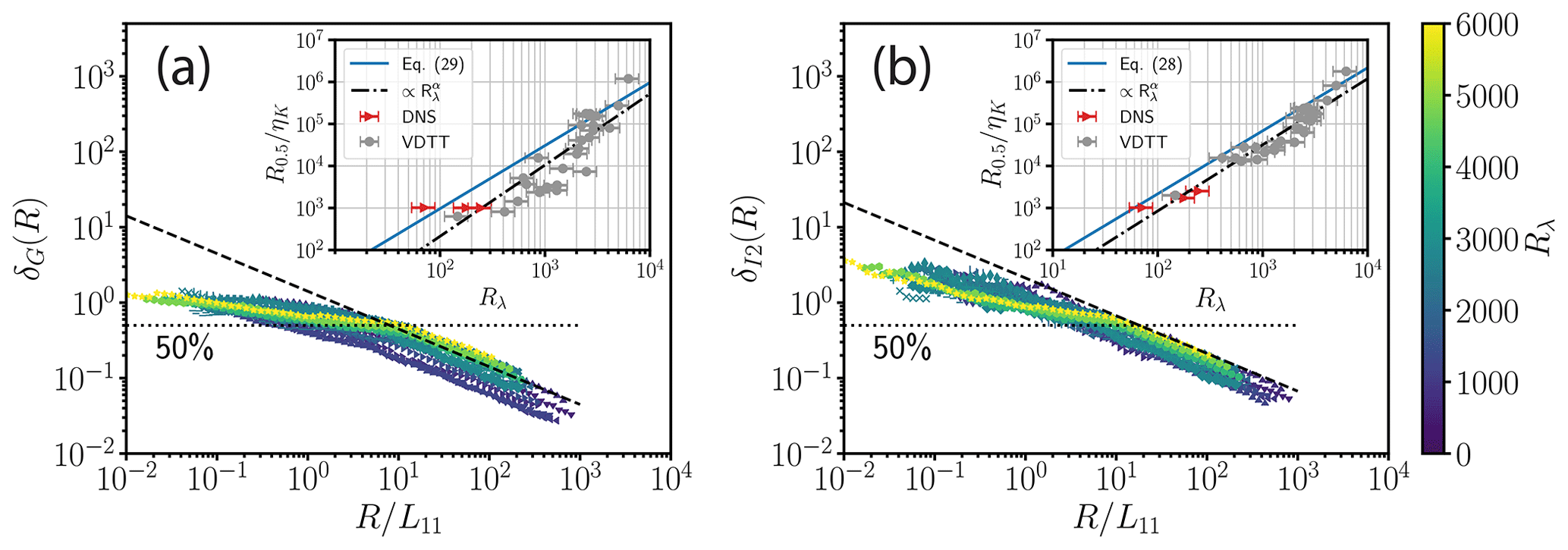
Figure 7 Random errors δ_G(R) (a) and δ_I2(R) (b) as a function of the re-scaled averaging window size $R/L_{\mathrm{11}}$ obtained from VDTT data at various R_λ values shown by the color bar. The analytical results for δ_G(R) (a, Eq. 25) and δ_I2(R) (b, Eq. 24) are shown by the dashed black lines. The dotted black line annotated with 50 % in each subplot corresponds to a 50 % error threshold. The insets show the sizes of the averaging windows in terms of η_K when ${\mathit{\delta }}_{G,I\mathrm{2}}\left(R\right)\le \mathrm{0.5}$ as a function of the Taylor-microscale Reynolds number R_λ. The inset plots include data from both the DNS (red triangles) and the VDTT (grey circles). DNS data used for the inset plots are from cases 1.3, 2.3 and 3.3 with I=10 % and θ=0^∘. The solid blue lines show the prediction of the required averaging window according to Eq. (29) (a – inset) and Eq. (28) (b – inset). The black dash-dotted line in the inset plots is a fit to the data: $\log R/{\mathit{\eta }}_K=\frac{\mathrm{3}}{\mathrm{4}}\log \frac{\mathrm{3}}{\mathrm{20}}-\mathrm{2}\log a_{\mathrm{fit}}+\mathit{\alpha }\log R_{\mathit{\lambda }}$, yielding $\mathit{\alpha }=\mathrm{1.70}\pm \mathrm{0.18}$ and $a_{\mathrm{fit}}=\mathrm{1.67}\pm \mathrm{0.64}$ (a – inset); $\log R/{\mathit{\eta }}_K=\log \frac{\mathrm{9}}{\mathrm{4}}{\frac{\mathrm{3}}{\mathrm{20}}}^{\mathrm{3}/\mathrm{4}}-\mathrm{2}\log a_{\mathrm{fit}}+\mathit{\alpha }\log R_{\mathit{\lambda }}$, yielding $\mathit{\alpha }=\mathrm{1.57}\pm \mathrm{0.09}$ and $a_{\mathrm{fit}}=\mathrm{0.95}\pm \mathrm{0.32}$ (b – inset).

The scaling of δ_G(R) and δ_I2(R) is predicted well for R≳10L₁₁ as expected from Eqs. (25) and (24) and the assumptions we made to derive them. However, for smaller R a statistical convergence of ϵ_G, ϵ_I2 or ϵ_L against the mean energy dissipation rate cannot be expected, in particular if $R/L_{\mathrm{11}}<\mathrm{1}$.

Furthermore, it is evident from Fig. 7 that the random errors do not fully collapse on each other for different Reynolds numbers and at a given $R/L_{\mathrm{11}}$. Moving horizontally on a line of constant random error, e.g., the dashed line of 50 % error, the required window size increases with R_λ, as shown in the insets of Fig. 7a and b. Predictions of Eqs. (28) and (29) are also shown in these plots via solid blue lines.

For both ϵ_G and ϵ_I2, the theoretical expectation for R_a tends to overestimate the actual averaging window size at which a random error of 50 % is achieved. This overestimation is expected as the theoretical expectation for R_a in Eqs. (28) and (29) is derived assuming that large-scale quantities such as f(r) and L₁₁ are fully converged. However, ϵ_G is technically relying on small scales. ϵ_G depends on velocity fluctuation gradients, which are numerically obtained by central differences. Hence, each increment in the velocity record contributes to the average in the gradient method (Eq. 6). In the case of ϵ_I2, the number of possible increments reduces for larger separations for a finite averaging window. By definition, the exact computation of L₁₁ even requires a fully converged f(r) for all r values.

However, VDTT experiments with R_λ>3000 underestimate the prediction of Eq. (20) by about a factor of 2. This is particularly clear for ϵ_L shown in Fig. A5. This deviation at high R_λ can be explained, at least in part, by the strong assumptions made for the derivation of the random errors, i.e., Eqs. (24), (22) and (25). In particular, for experiments with high Re in VDTT, the assumption of Gaussian velocity fluctuations with zero skewness is questionable, as shown in Fig. A6. Lenschow et al. (1994) have already established that the size of the averaging window for a skewed Gaussian process (see Eq. 19 in Lenschow et al., 1994) must be twice as large as for a Gaussian process with vanishing skewness. However, further work is needed to investigate these deviations and improve the theoretical prediction.

3.6 Estimating the transient energy dissipation rate

As has been shown previously in Figs. 6 and 7, both systematic and random errors decrease with the size of the averaging window. For a correct estimate of the magnitude, it is therefore advantageous to choose the averaging window as large as possible, but the price of this is that the transient trend smaller than the selected window size cannot be reproduced. In addition, it is also important to know to what extent statistical uncertainties originating from the estimation methods themselves disguise the true trends of the underlying turbulent flow. Given a certain averaging window size R, here, we empirically evaluate if trends in the coarse-grained time series are physical or rather statistical. In other words, we ask the question whether local estimates of the mean energy dissipation rate follow the ground-truth reference $\langle {\mathit{ϵ}}_{\mathrm{0}}(\mathit{x},t){\rangle }_{\mathrm{VP},R}$ or not. Respecting the intermittent nature of turbulence and energy dissipation, the standard deviation of $\langle {\mathit{ϵ}}_{\mathrm{0}}(\mathit{x},t){\rangle }_{\mathrm{VP},R}$ is a first proxy for the variability of the trend in $\langle {\mathit{ϵ}}_{\mathrm{0}}(\mathit{x},t){\rangle }_{\mathrm{VP},R}$. Hence, detecting the true trend requires that β_i and δ_i(R) are smaller than the standard deviation of $\langle {\mathit{ϵ}}_{\mathrm{0}}(\mathit{x},t){\rangle }_{\mathrm{VP},R}$.

It can already be concluded from Figs. 2, 7, A1 and A5 that ϵ_G is the most promising candidate to capture the true trend. However, to fully answer the above questions, we need to conduct a more in-depth analysis. The upper plot in Fig. 8 shows the re-scaled and coarse-grained dissipation field $\langle {\mathit{ϵ}}_{\mathrm{0}}(\mathit{x},t){\rangle }_{\mathrm{VP},R}$ for a sliding window of size R≈5500η_K and a turbulence intensity I=10 % obtained from the time series of one virtual probe for case DNS 2.0 (“probe 0”). Consistent with results shown earlier, 〈ϵ_G〉_R follows $\langle {\mathit{ϵ}}_{\mathrm{0}}(\mathit{x},t){\rangle }_{\mathrm{VP},R}$ best in comparison with 〈ϵ_I2〉_R and 〈ϵ_L〉_R. Both 〈ϵ_I2〉_R and 〈ϵ_L〉_R are associated with substantial scatter, although 〈ϵ_I2〉_R has smaller deviations from the ground truth overall. Other probe tracks sample different portions of the flow, which is why a quantitative conclusion is not possible from one single probe. A more comprehensive evaluation of which method is able to capture the true trend is conducted below.

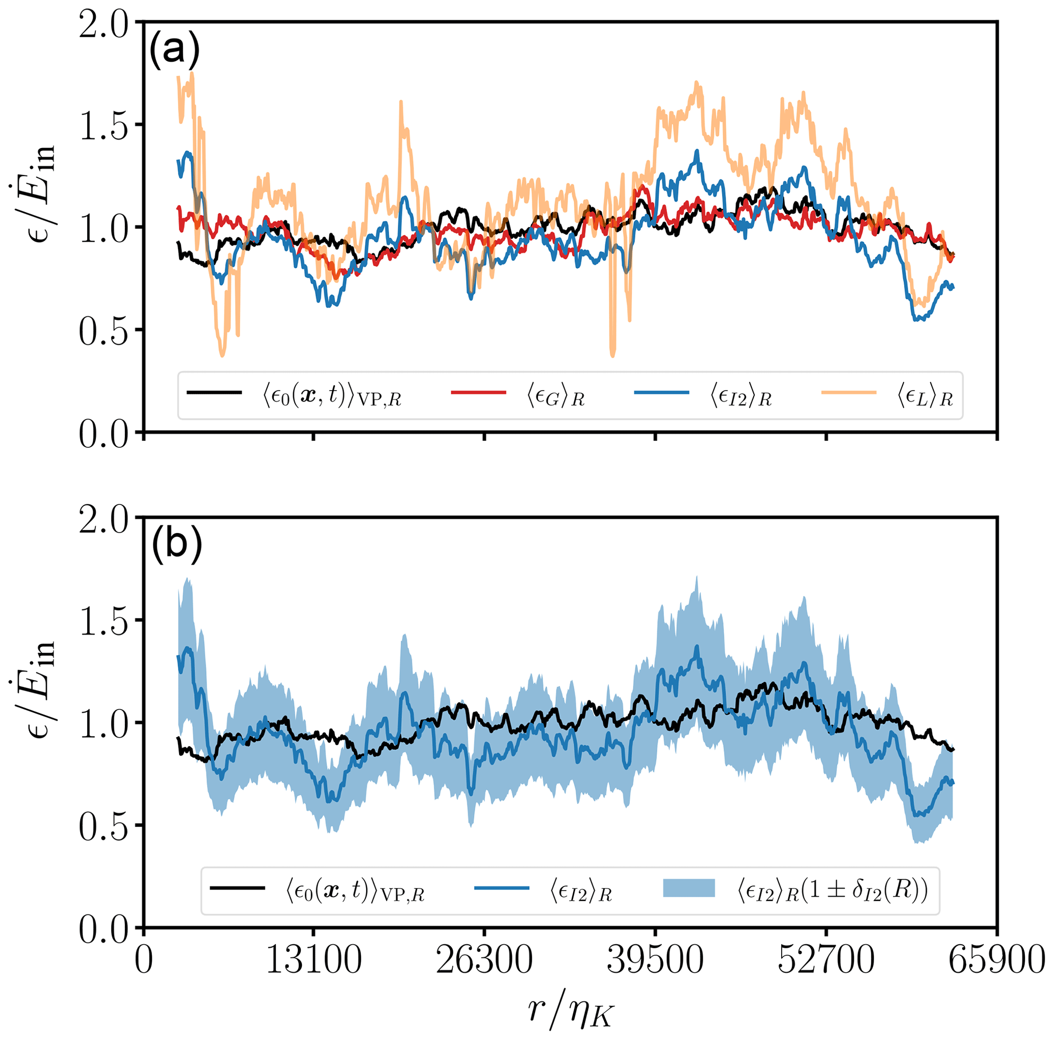
Figure 8 (a) Proof of concept for estimating the coarse-grained energy dissipation rate $\langle {\mathit{ϵ}}_{\mathrm{0}}(\mathit{x},t){\rangle }_{\mathrm{VP},R}$ re-scaled by the energy injection rate ${\dot{E}}_{\mathrm{in}}$ via the one-dimensional surrogates 〈ϵ_G〉_R, 〈ϵ_I2〉_R and 〈ϵ_L〉_R for R_λ=142, $R/{\mathit{\eta }}_K\approx \mathrm{5500}$, θ=0^∘ and a turbulence intensity I=10 % (DNS 2.0). All estimates are re-scaled by the energy injection rate ${\dot{E}}_{\mathrm{in}}$, too. We narrowed the fit range to $\mathrm{20}{\mathit{\eta }}_K\le r\le \mathrm{200}{\mathit{\eta }}_K$, ensuring optimal fit results. (b) Comparison between $\langle {\mathit{ϵ}}_{I\mathrm{2}}{\rangle }_R/{\dot{E}}_{\mathrm{in}}$ with the estimated random error according to Eq. (24) for the averaging window R and $\langle {\mathit{ϵ}}_{\mathrm{0}}(\mathit{x},t){\rangle }_{\mathrm{VP},R}$.

The lower plot in Fig. 8 shows 〈ϵ_I2〉_R together with the random error of ϵ_I2 as defined by Eq. (24). Despite the strong scatter, the ground-truth reference is nearly always within the error bar of ϵ_I2, with some exceptions, e.g., $r/{\mathit{\eta }}_K<\mathrm{5000}$ or $r/{\mathit{\eta }}_K\approx$ 60 000. It can also be seen that 〈ϵ_I2〉_R is, if at all, only weakly correlated with the ground-truth reference $\langle {\mathit{ϵ}}_{\mathrm{0}}(\mathit{x},t){\rangle }_{\mathrm{VP},R}$ for a window size of $R/{\mathit{\eta }}_K\approx \mathrm{5500}$. This shows that it is extremely difficult, if at all possible, to track the true trend with low-resolution time records.

To assess this correlation more quantitatively, we evaluate the Pearson correlation coefficient between the ground-truth reference $\langle {\mathit{ϵ}}_{\mathrm{0}}(\mathit{x},t){\rangle }_{\mathrm{VP},R}$ and ϵ_G, ϵ_I2 as well as ϵ_L, respectively, as a function of the re-scaled averaging window size $R/{\mathit{\eta }}_K$ for all virtual probes of case DNS 2.0. As an example, the Pearson correlation coefficient between ϵ₀(x,t)〉_R and ϵ_I2 is 0.33 in Fig. 8 (upper plot). Figure 9a shows the ensemble averages of the Pearson correlation coefficient together with the standard error (shaded area). While 〈ϵ_G〉_R has a pronounced correlation with the ground-truth reference $\langle {\mathit{ϵ}}_{\mathrm{0}}(\mathit{x},t){\rangle }_{\mathrm{VP},R}$, both 〈ϵ_I2〉_R and 〈ϵ_L〉_R are only very weakly correlated with 〈ϵ_G〉_R.

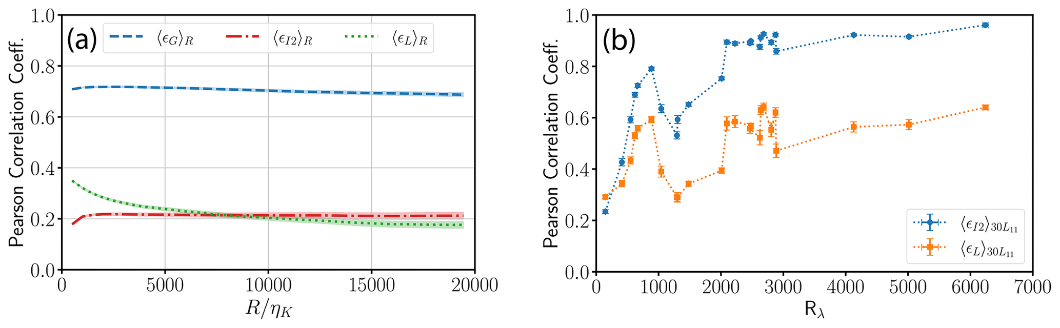
Figure 9 (a) Dependence of the Pearson correlation coefficient between 〈ϵ_i〉_R and $\langle {\mathit{ϵ}}_{\mathrm{0}}(\mathit{x},t){\rangle }_{\mathrm{VP},R}$ as a function of the re-scaled averaging window $R/{\mathit{\eta }}_K$ where $i\in \mathit{\{}G,I\mathrm{2},L\mathit{\}}$. Time records of the longitudinal velocity by all virtual probes and $\langle {\mathit{ϵ}}_{\mathrm{0}}(\mathit{x},t){\rangle }_{\mathrm{VP},R}$ are taken from DNS 2.0 with R_λ=142, turbulence intensity I=10 % and perfect alignment (θ=0^∘). The shaded region is given by the standard error. (b) Dependence of the Pearson correlation coefficient between 〈ϵ_I2,L〉_R and 〈ϵ_G〉_R as a function R_λ for a fixed re-scaled averaging window R=30L₁₁. The error bars of the ensemble-averaged coefficients are given by the standard error.

The effect of R_λ on the Pearson correlation coefficient is also shown in Fig. 9b for the VDTT experiments at various R_λ values. Here, we compare ϵ_I2 and ϵ_L to ϵ_G in the absence of a ground-truth reference. To ensure a negligible systematic error, we chose a fixed averaging window of R=30L₁₁ for each R_λ. Figure 9b shows that the correlation for ϵ_I2 is always higher than that of ϵ_L, except for very low R_λ. There is a non-monotonic behavior in the correlation coefficients in Fig. 9b that seems to be related to the skewness values shown in Fig. A6. Nonetheless, there is a clear increase in correlation coefficients with R_λ. Firstly, the random error in δ_I2(R) ranges from 20 % to 40 % at R=30L₁₁. Secondly, the kurtosis of the instantaneous energy dissipation field scales with $R_{\mathit{\lambda }}^{\mathrm{3}/\mathrm{2}}$ (Pope, 2000), which is why the variability in the instantaneous energy dissipation field increases with R_λ. Hence, at small $R_{\mathit{\lambda }}^{\mathrm{3}/\mathrm{2}}$ and R=30L₁₁, $\langle {\mathit{ϵ}}_{I\mathrm{2}}{\rangle }_{\mathrm{30}{L}_{\mathrm{11}}}$ scatters only randomly around the global mean energy dissipation rate (with a 3 % standard deviation of $\langle {\mathit{ϵ}}_G{\rangle }_{\mathrm{30}{L}_{\mathrm{11}}}$), which is why the correlation coefficient is low. In contrast, at large R_λ and R=30L₁₁, the locally averaged mean energy dissipation rate $\langle {\mathit{ϵ}}_G{\rangle }_{\mathrm{30}{L}_{\mathrm{11}}}$ fluctuates more strongly (≈30 % standard deviation of $\langle {\mathit{ϵ}}_G{\rangle }_{\mathrm{30}{L}_{\mathrm{11}}}$) where δ_I2(R) is already comparable.

4 Practical guidelines

Up to this point, we have presented the results largely as is so that one can interpret them with minimal bias. However, the amount of data and details given may make the use of the results in practice difficult. Therefore, we propose here practical guidelines for measuring the energy dissipation rate from one-dimensional velocity records in atmospheric flows.

The gradient method should be preferred over other methods for conditions where the turbulence intensity is low and where the probe could be perfectly aligned in the direction of the mean wind. In particular, the gradient method is more sensitive to turbulence intensity than inertial-range methods due to random-sweeping effects. Low values of turbulence intensity and ideal alignment of probes can be best controlled in ground-based measurements. Measurements aboard research aircraft traveling at a true speed of 100 m s⁻¹ can also satisfy these conditions, but the spatial and temporal resolution required to measure the velocity gradients (see Fig. A8) is challenging to achieve; i.e., a robust probe with a wire length ideally smaller than 1 mm (or of the same order as η_K) and a true response frequency of 10⁵ Hz are needed. Other airborne platforms, such as helicopters, balloons and kites, would encounter higher turbulence intensities, making Taylor's frozen flow assumption more difficult to satisfy. Most importantly, however, they all suffer from probe alignment into the local wind at the scale of the measurement platform.

Other estimates based on inertial-sub-range methods (cf. Table 1) are less sensitive to a high turbulence intensity and probe alignment. Regarding the impact of a high turbulence intensity, we find the most reliable method for most field applications to be the second-order structure function. However the accuracy is at least 10 %, even in most ideal conditions considered here (Table 4). Considering experimental imperfections, the actual deviation is expected to be of the order of 100 % (Figs. 3 and 5).

Given atmospheric turbulence with η_K∼1 mm and L₁₁∼100 m, the inertial range of the second-order structure function extends from about 60η_K (Pope, 2000) to at most the integral scale, if at all. However, for applying the second-order SF method (inertial range), at least 1 to 2 decades of the inertial range are needed. Assuming that the fitting range is chosen from 0.1 to 10 m, a measurement platform with a true air speed of 10–100 m s⁻¹ requires an anemometer with a sampling frequency of 100–1000 Hz in order to provide about 2 decades of data within the inertial range.

Our analysis further shows that estimating the transient energy dissipation in atmospheric clouds (L₁₁∼100 m, 𝒪(R_λ)∼10³–10⁴) via the second-order structure function (inertial range) with an averaging window of R=100 m is prone to random errors of the order of 100 % (Fig. 7b). Shorter averaging windows involve even higher random errors. It is therefore recommended to choose the averaging window as large as possible but still smaller than length and timescales on which the atmosphere remains homogeneous and stationary, respectively. This recommendation is not easy to achieve in an atmosphere. For example, measurements in the marine boundary layer with intermittent shallow cumulus clouds require a careful consideration in regard to stationary conditions. Then, two approaches can be recommended. On the one hand, one can choose a very long averaging window to average over many individual clouds associated with a small random error but potentially violating the stationary and homogeneity condition. On the other hand, one could investigate the transient mean energy dissipation rate (as a proxy for the local mean energy dissipation rate per cloud), while accepting a large random error.

The large random errors also preclude the possibility of interpreting trends in the measured energy dissipation rate via the second-order structure function if we consider the results shown in Figs. 8 and 9a. Even if we consider the promising correlations shown in Fig. 9b at high Reynolds numbers, interpreting trends and patterns in atmospheric data from one-dimensional time records remains a challenge, especially in an atmosphere with intermittent cloudiness. As an example, in a cloud with a horizontal extent of 1 km, one can obtain 10 non-overlapping data blocks with a window length of 100 m, which corresponds to a random error of about 100 % to be combined with a systematic error of the same order of magnitude. With 10 data points combined with such large uncertainties, it would be extremely difficult to interpret the change in the dissipation rate in this cloud. Interpretations of trends in the energy dissipation rate would be particularly flawed if the size of the averaging window is <10L₁₁. At best, one average value can be determined for such small clouds, which would still deviate from the global mean by at least 50 %–100 % if (and this is a big if) the cloud is sufficiently stationary and homogeneous for averaging. However, the limitations imposed by the validity of the Taylor hypothesis can be mitigated by using an array of high-resolution anemometers. The array should be oriented so that the anemometers point in the mean local wind direction. The calculation of transverse velocity gradients or second-order structure functions would no longer depend on the applicability of the Taylor hypothesis, since the distances between the sensors are predefined by the design.

5 Summary

We have presented an extensive review on the analysis procedure for estimating the energy dissipation rate from single-point one-dimensional velocity time records along with an overview of the advantages and disadvantages (see Table 1). To conclude, this paper provides means to estimate errors in the global and local mean energy dissipation rates due to experimental imperfections and limitations. These estimated errors can be used to assess the quality and accuracy of the measurement. Furthermore, error estimates of the global and local mean energy dissipation rates can be used to assess the errors in other turbulence and cloud droplet parameters, e.g., various turbulence length scales and the cloud droplet Stokes number, with the help of Gaussian error propagation. A set of practical guidelines for measurement and analysis strategies has been provided in the previous section, and the following presents a technical summary of the main results.

The main methods considered in this study are the gradient method ϵ_G, the second-order SF (inertial-range) method ϵ_I2, the spectral method ϵ_S and the scaling argument ϵ_L. We have provided a systematic assessment of the accuracy of inferring the energy dissipation rate from such one-dimensional velocity time series as a function of turbulence intensity, probe orientation with respect to the longitudinal direction and the effect of a finite averaging window size. We used DNS data with Reynolds numbers in the range $\mathrm{74}\le R_{\mathit{\lambda }}\le \mathrm{321}$ as well as experimental data from high-resolution one-dimensional wind tunnel measurements with Reynolds numbers in the range $\mathrm{147}\le R_{\mathit{\lambda }}\le \mathrm{5864}$ to evaluate the performance of different methods against robust benchmark values. The results presented in this study help to assess the accuracy of the energy-dissipation-rate estimates as a function of several parameters, such as finite turbulence intensity, misalignment between sensor and longitudinal flow direction, and finite size of the averaging window. The main results are as follows:

• Each method could reproduce the ground-truth reference 〈ϵ(x,t)〉 to within less than 10 % for well-converged statistics and at low turbulence intensity. The most accurate method is the gradient method (ϵ_G), and the least accurate method is the one based on the $\mathrm{4}/\mathrm{5}$ law (ϵ_I3) (see Fig. 2). The reference-compared systematic error tends to be overestimated due to the global choice of the fit range; e.g., lower systematic errors for ϵ_I2 can be obtained by choosing a fit range for each DNS dataset that is in a range where the scaling of the structure function is closest to the expected scaling.

• In the case of finite turbulence intensities, ϵ_G, ϵ_S and ϵ_I2 systematically overestimate the ground-truth energy dissipation rate. The gradient method (ϵ_G) is the most affected by a finite turbulence intensity I, whereas ϵ_I2 is the least affected (see Figs. 3 and 4b). The overestimation can be captured by a random-advection model (Fig. 4). Regarding the small-scale estimate ϵ_G, the error formula provided by Lumley (1965) (β_G∝5I²) captures the effect of random advection.

• Considering the probe orientation, the gradient method (ϵ_G) is the most affected by misalignment between the probe orientation and the longitudinal flow direction, whereas ϵ_I2 is the least affected (Fig. 5) (compare Eqs. 19, 17 and 18).

• We provide scaling arguments δ_i(R) to estimate the required averaging window size optimized for a desired random-error threshold for ϵ_G in Eq. (29), ϵ_I2 in Eq. (28) and ϵ_L in Eq. (28). With this, we can estimate a coarse-grained energy dissipation rate to within a predicted uncertainty as shown in Fig. 8. Systematic errors β_i are smaller than random errors δ_i(R) for R>2L₁₁.

• The random error in the gradient method δ_G(R) converges at least 4–5 times faster than ϵ_I2 (compare Eqs. 28 and 29).

• Only ϵ_G estimates the transient energy dissipation rate 〈ϵ₀〉_R reliably, although it is the most vulnerable to experimental imperfections/limitations.

Appendix A: Preliminaries on second-order statistics

As discussed in detail below, the mean energy dissipation rate can be related to second-order statistics of the velocity field, either in terms of velocity gradients or in terms of velocity increments. In any case, the two-point velocity covariance tensor turns out to be the central quantity of interest from which the second-order structure function tensor, the spectral energy tensor and the velocity gradient covariance tensor can be obtained.

In the following, we assume a zero mean SHI turbulence so that two-point quantities depend only on the separation vector r. All averages are invariant under rotations of the coordinate system, and the mean squared velocity fluctuation is identical for all velocity components; i.e., $\langle u^{\prime \mathrm{2}}\rangle =\langle u_{\mathrm{1}}^{\prime \mathrm{2}}\rangle =\langle u_{\mathrm{2}}^{\prime \mathrm{2}}\rangle =\langle u_{\mathrm{3}}^{\prime \mathrm{2}}\rangle$. We provide an overview of the most relevant definitions, their notations and their conventions. This section does not explicitly discuss the effect of the averaging window, but the definitions presented can be applied to windowed inputs with no or straightforward modifications.

Under the given assumptions, the two-point velocity covariance tensor takes the form (e.g., Pope, 2000; Robertson, 1940; Batchelor, 1953)

$$\begin{array}{}\text{(A1)}& \begin{array}{rl}{R}_{ij}\left(\mathit{r}\right)& =\langle u_i^{\prime }(\mathit{x}+\mathit{r},t)u_j^{\prime }(\mathit{x},t)\rangle \\ & =\langle u^{\prime \mathrm{2}}\rangle \left(g\left(r\right){\mathit{\delta }}_{ij}+\left[f\left(r\right)-g\left(r\right)\right]{\displaystyle \frac{r_i{r}_j}{r^{\mathrm{2}}}}\right),\end{array}\end{array}$$

where $f\left(r\right)=R_{\mathrm{11}}\left(r\right)/R_{\mathrm{11}}\left(\mathrm{0}\right)$ and $g\left(r\right)=f\left(r\right)+r{\partial }_{r}f\left(r\right)/\mathrm{2}$ are the longitudinal and transverse autocorrelation functions, respectively, with $f\left(\mathrm{0}\right)=g\left(\mathrm{0}\right)=\mathrm{1}$. Notably, if one chooses r=re₁, then $R_{\mathrm{11}}\left(r\right)=\langle u^{\prime \mathrm{2}}\rangle f\left(r\right)$ and $R_{\mathrm{22}}\left(r\right)=R_{\mathrm{33}}\left(r\right)=\langle u^{\prime \mathrm{2}}\rangle g\left(r\right)$ as well as all other components vanish (e.g., Pope, 2000). As a remarkable consequence, R_ij(r) is uniquely defined by f(r) in isotropic turbulence. As mentioned below, the integral length scale as well as the Taylor microscale are determined by f(r) (Pope, 2000).

Analogously, a covariance tensor can be defined for velocity increments, i.e., the second-order velocity structure function tensor (Pope, 2000; Davidson, 2015)

$$\begin{array}{}\text{(A2)}& \begin{array}{rl}& D_{ij}\left(\mathit{r}\right)\\ & =〈\left[u_i^{\prime }(\mathit{x}+\mathit{r},t)-u_i^{\prime }(\mathit{x},t)\right]\left[u_j^{\prime }(\mathit{x}+\mathit{r},t)-u_j^{\prime }(\mathit{x},t)\right]〉\\ & =D_{\mathrm{NN}}\left(r\right){\mathit{\delta }}_{ij}+\left[D_{\mathrm{LL}}\left(r\right)-D_{\mathrm{NN}}\left(r\right)\right]{\displaystyle \frac{r_i{r}_j}{r^{\mathrm{2}}}}.\end{array}\end{array}$$

The longitudinal second-order structure function D₁₁(r) is related to f(r) by (e.g., Pope, 2000; Davidson, 2015)

$$\begin{array}{}\text{(A3)}& \begin{array}{rl}{D}_{\mathrm{11}}(\mathit{r}=r{\mathit{e}}_{\mathrm{1}})& =D_{\mathrm{LL}}\left(r\right)\\ & =\langle \left(u_{\mathrm{1}}^{\prime }\right(\mathit{x}+r{\mathit{e}}_{\mathrm{1}},t)-u_{\mathrm{1}}^{\prime }(\mathit{x},t){)}^{\mathrm{2}}\rangle \\ & =\mathrm{2}\langle u^{\prime \mathrm{2}}\rangle (\mathrm{1}-f(r\left)\right).\end{array}\end{array}$$

As explained below, by measuring the longitudinal second-order structure function D_LL(r), the mean energy dissipation rate can be inferred from the inertial-range scaling of the longitudinal structure function (cf. Eq. 7).

Furthermore, the velocity gradient covariance tensor can also be defined in terms of the velocity covariance tensor

$$\begin{array}{}\text{(A4)}& R_{ijkl}\left(\mathit{r}\right)=〈{\displaystyle \frac{\partial u_i^{\prime }(\mathit{x},t)}{\partial x_k}}{\displaystyle \frac{\partial u_j^{\prime }({\mathit{x}}^{\prime },t)}{\partial x_l^{\prime }}}〉=-{\partial }_{r_k}{\partial }_{r_l}{R}_{ij}\left(\mathit{r}\right).\end{array}$$

Since the local and instantaneous energy dissipation rate (cf. Eq. 3) is defined in terms of the strain-rate tensor $S_{ik}=\left(\partial u_i^{\prime }(\mathit{x},t)/\partial x_k+\partial u_k^{\prime }(\mathit{x},t)/\partial x_i\right)/\mathrm{2}$, the mean energy dissipation rate can be directly related to contractions of the velocity gradient covariance tensor evaluated at zero. Note that in a turbulent flow with a zero mean velocity, the strain-rate tensor S_ik is equal to the fluctuation strain-rate tensor s_ik.

The two-point velocity covariance tensor can be expressed in Fourier space through the energy spectrum tensor (Pope, 2000)

$$\begin{array}{}\text{(A5)}& {\mathrm{\Phi }}_{ij}\left(\mathit{\kappa }\right)={\displaystyle \frac{\mathrm{1}}{(\mathrm{2}\mathit{\pi }{)}^{\mathrm{3}}}}\underset{-\mathrm{\infty }}{\overset{+\mathrm{\infty }}{\iiint }}{R}_{ij}\left(\mathit{r}\right)e^{-i\mathit{\kappa }\cdot \mathit{r}}\mathrm{d}\mathit{r},\end{array}$$

where κ is the wave vector. For SHI turbulence, Φ_ij(κ) takes the form

$$\begin{array}{}\text{(A6)}& {\mathrm{\Phi }}_{ij}\left(\mathit{\kappa }\right)={\displaystyle \frac{E\left(\mathit{\kappa }\right)}{\mathrm{4}\mathit{\pi }{\mathit{\kappa }}^{\mathrm{2}}}}\left({\mathit{\delta }}_{ij}-{\displaystyle \frac{{\mathit{\kappa }}_i{\mathit{\kappa }}_j}{{\mathit{\kappa }}^{\mathrm{2}}}}\right),\end{array}$$

where E(κ) is the energy spectrum function.

Since access to the full energy spectrum function is not always available, one-dimensional spectra are of interest, too. The mean energy dissipation rate can be estimated from the inertial-range scaling of the longitudinal one-dimensional spectrum (as shown in Eq. 9), which can be calculated by both the energy spectrum function and the velocity covariance tensor (Pope, 2000)

$$\begin{array}{}\text{(A7)}& \begin{array}{rl}{E}_{\mathrm{11}}\left({\mathit{\kappa }}_{\mathrm{1}}\right)& =\underset{{\mathit{\kappa }}_{\mathrm{1}}}{\overset{\mathrm{\infty }}{\int }}{\displaystyle \frac{E\left(\mathit{\kappa }\right)}{\mathit{\kappa }}}\left(\mathrm{1}-{\displaystyle \frac{{\mathit{\kappa }}_{\mathrm{1}}^{\mathrm{2}}}{{\mathit{\kappa }}^{\mathrm{2}}}}\right)\mathrm{d}\mathit{\kappa }\\ & ={\displaystyle \frac{\mathrm{1}}{\mathit{\pi }}}\underset{-\mathrm{\infty }}{\overset{\mathrm{\infty }}{\int }}{R}_{\mathrm{11}}\left({\mathit{e}}_{\mathrm{1}}{r}_{\mathrm{1}}\right)e^{-i{\mathit{\kappa }}_{\mathrm{1}}{r}_{\mathrm{1}}}\mathrm{d}{r}_{\mathrm{1}},\end{array}\end{array}$$

with the wavenumber κ₁ corresponding to the e₁ direction and $R_{\mathrm{11}}\left(\mathrm{0}\right)=\langle u^{\prime \mathrm{2}}\rangle ={\int }_{\mathrm{0}}^{\mathrm{\infty }}{E}_{\mathrm{11}}\left({\mathit{\kappa }}_{\mathrm{1}}\right)\mathrm{d}{\mathit{\kappa }}_{\mathrm{1}}$.

This concludes the second-order statistics in terms of the velocity that we consider in the main text to determine the mean energy dissipation rate.

Table A1 Nomenclature for the turbulent flow. If our naming convention differs from the terminology in Pope (2000), we add the convention of Pope (2000) in parentheses. Equations are either directly given or referenced from definitions below.

Table A2 Nomenclature for the subscripts.

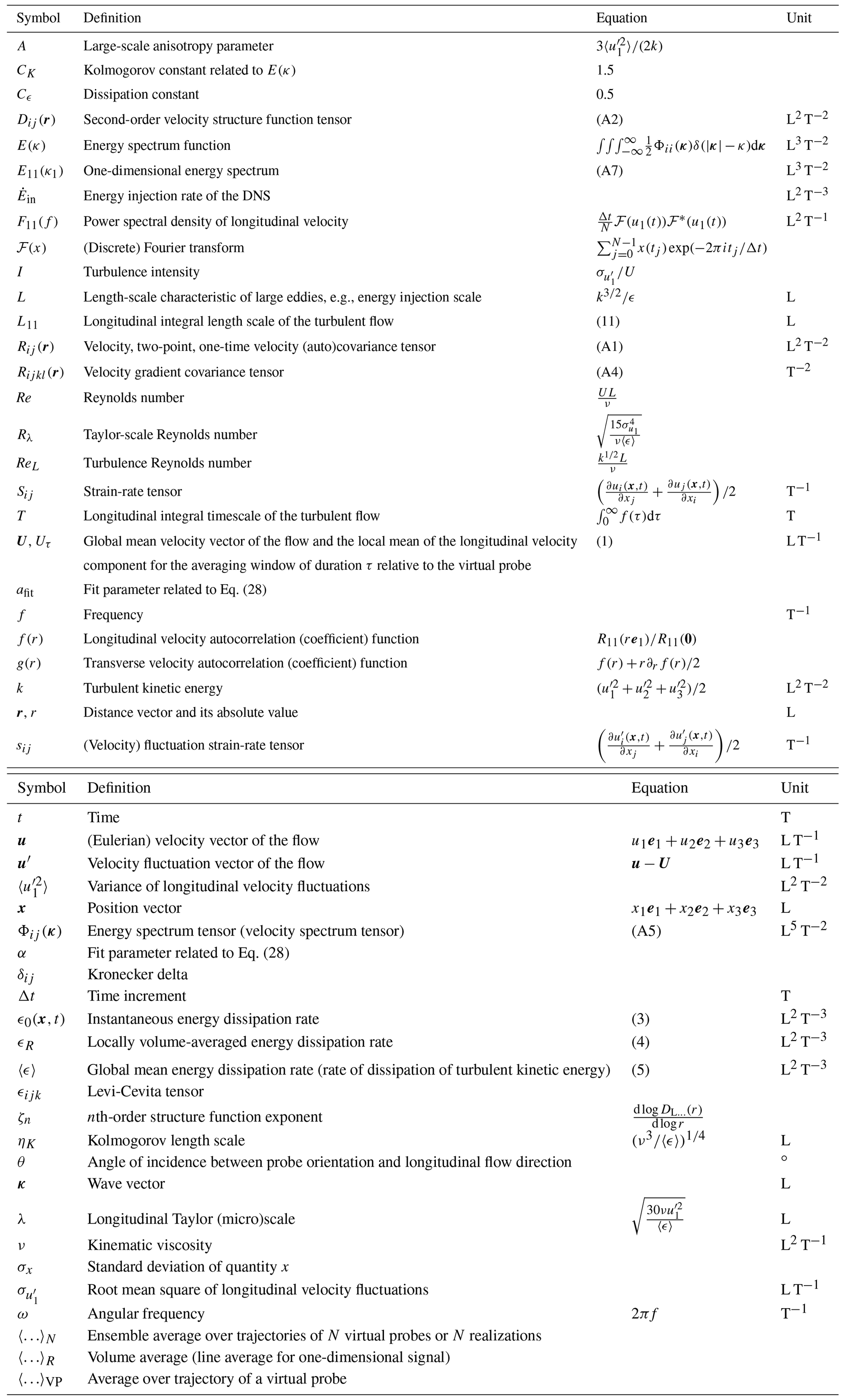
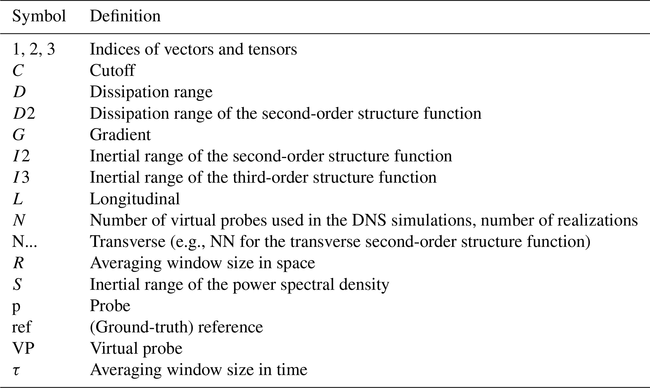
Table A3 The systematic error in each method β_i relative to the global mean energy dissipation rate in Eq. (12) of each DNS where $i\in \mathit{\{}G,I\mathrm{3},I\mathrm{2},S,L\mathit{\}}$. The error is given by the standard error, which is defined as the standard deviation divided by the square root of the number of samples. In both DNS 2.1 and DNS 3.1, ϵ_I2 and ϵ_I3 were obtained by fitting Eq. (7) for n=2 and n=3, respectively, in the range $r\in \left[\mathrm{20}{\mathit{\eta }}_K,\mathrm{500}{\mathit{\eta }}_K\right]$. This fit range is also used for calculating ϵ_S, and it was converted into the frequency domain by $f=U/r$, where U is the mean velocity. In the case of DNS 1.1, the maximum of Eq. (7) was used to infer ϵ_I2 due to the absence of a pronounced inertial range. We used the maximum available window size R in all cases and fixed turbulence intensity I=1 % and considered perfect alignment; i.e., θ=0^∘.

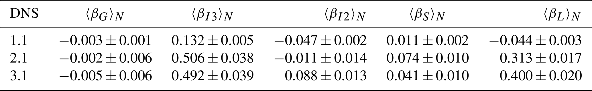
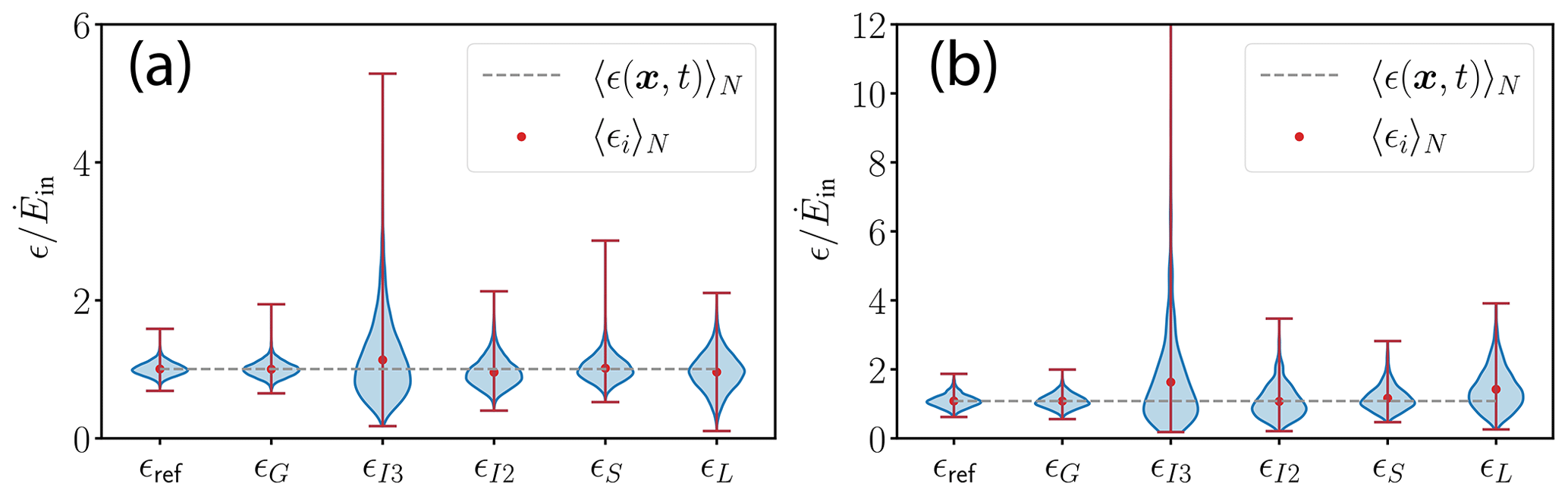
Figure A1 Validation of estimating the energy dissipation rate from ${\mathit{ϵ}}_G,{\mathit{ϵ}}_{I\mathrm{2}},{\mathit{ϵ}}_{I\mathrm{3}},{\mathit{ϵ}}_S$ and ϵ_L. All estimates are re-scaled by the energy injection rate ${\dot{E}}_{\mathrm{in}}$. The data are taken from DNS 1.1 (a) and 2.1 (b); turbulence intensity I=1 %. The ensemble mean of each method 〈ϵ_i〉_N is denoted by red dots where the whiskers extend from the minimal to maximal estimate of ϵ_i where $i\in \mathit{\{}G,I\mathrm{3},I\mathrm{2},S,L\mathit{\}}$. As the inertial range of DNS 1.1 (I=1 %, θ=0^∘ and maximal available averaging window) is not pronounced well due to the low R_λ∼74, we used the maximum of Eq. (7) in order to retrieve ϵ_I2,3. The dashed line represents the global mean energy dissipation rate of DNS 1.1 and 2.1 (R_λ=219, I=1 %, θ=0^∘ and maximal available averaging window), respectively, which is approximated by the ensemble average of the true mean energy dissipation rate along the trajectory of each virtual probe. ϵ_ref is the reference distribution of the ground-truth global mean energy dissipation field originating from the dissipation field along the trajectory of each virtual probe.

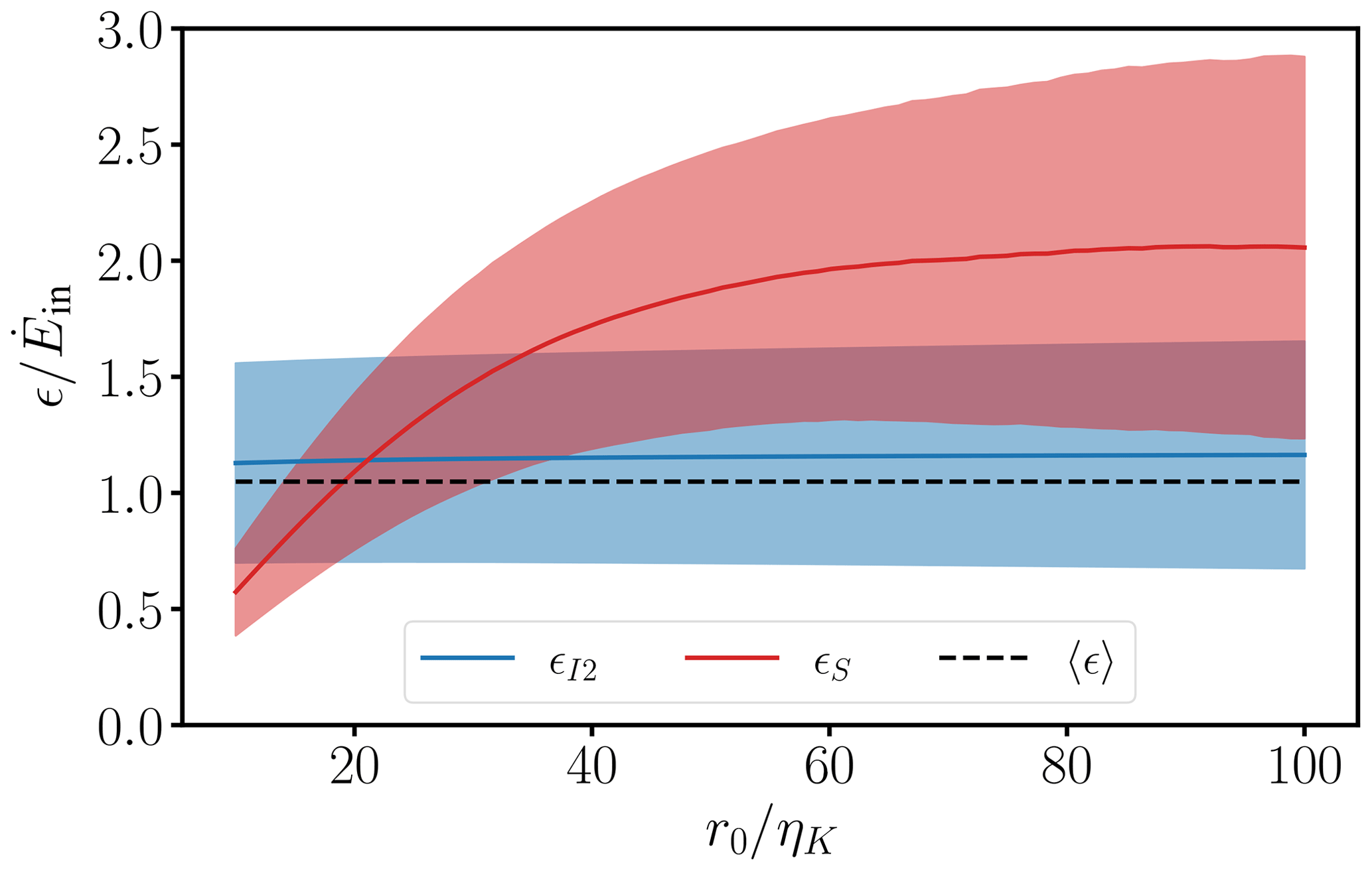
Figure A2 Estimates of the mean energy dissipation rate as a function of the fit range for ϵ_I2 and ϵ_S for DNS 3.1 (1000 probes, R_λ=302, I=1 %, θ=0^∘ and maximal available averaging window) re-scaled by the energy injection rate ${\dot{E}}_{\mathrm{in}}$. The solid line represents the ensemble average, whereas the shaded region is given by the standard deviation. $r_{\mathrm{0}}\in [\mathrm{10}{\mathit{\eta }}_K,\mathrm{100}{\mathit{\eta }}_K]$ is the lower boundary of the fit range for ϵ_I2 where the upper boundary is fixed at r₁=500η_K. For ϵ_S, the fit range is given by $f\in [U/r_{\mathrm{1}},U/r_{\mathrm{0}}]$. The dashed line denotes the global mean energy dissipation rate.

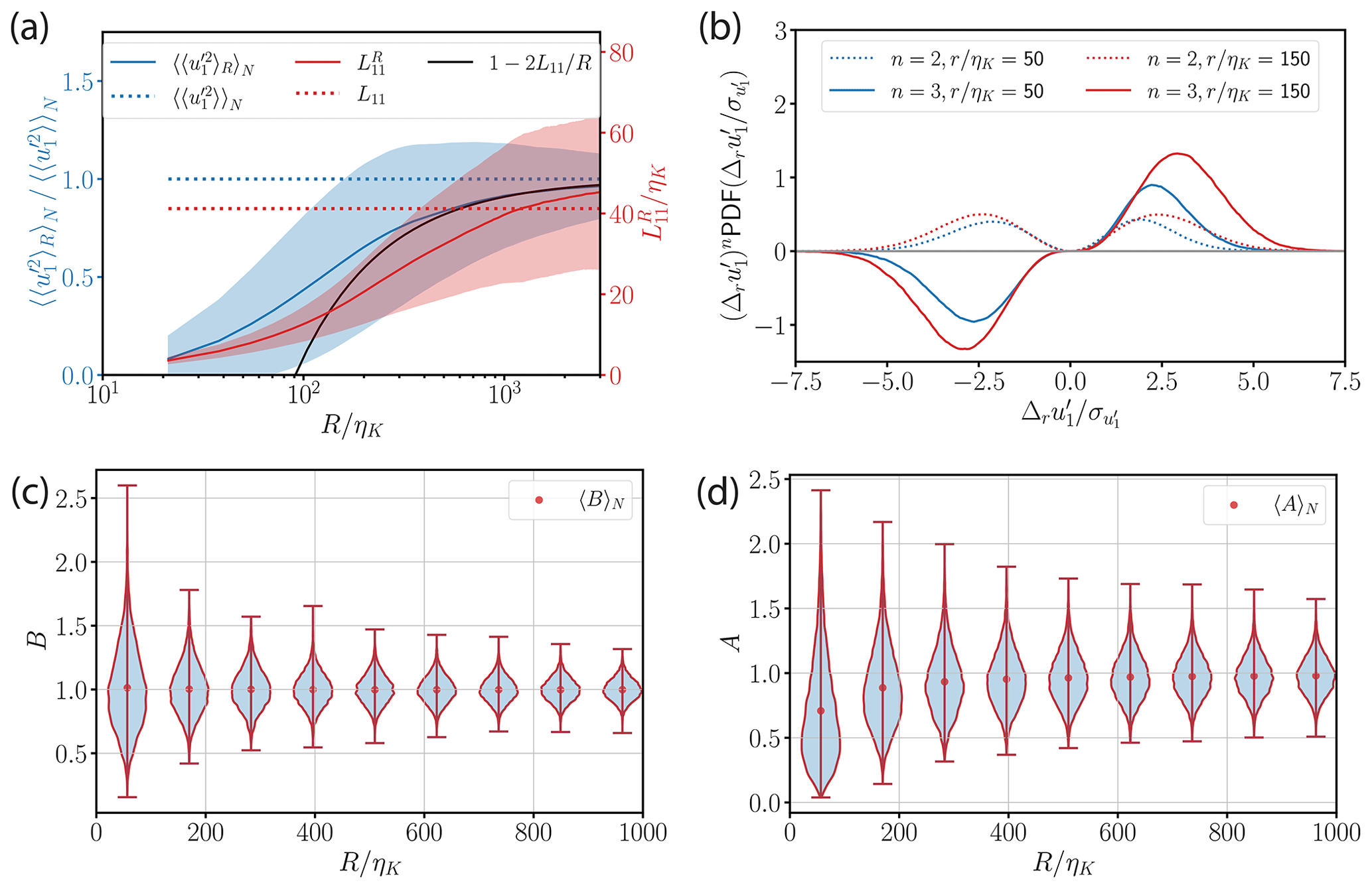
Figure A3 Convergence of higher-order statistical quantities and longitudinal integral length scales as well as small- and large-scale anisotropy obtained from all virtual probes of DNS 1.1 (R_λ=74, I=1 %, θ=0^∘). (a) The variance of the longitudinal velocity fluctuations $\langle u_{\mathrm{1}}^{\prime \mathrm{2}}\rangle$ and the longitudinal integral length scale $L_{\mathrm{11}}^R$ as a function of the averaging window size R normalized by the Kolmogorov length scale η_K. $\langle u_{\mathrm{1}}^{\prime \mathrm{2}}\rangle$ is re-scaled by the ensemble-averaged variance of the longitudinal velocity fluctuations. For large R, $\langle \langle u_{\mathrm{1}}^{\prime \mathrm{2}}{\rangle }_R{\rangle }_N$ converges to $\langle u_{\mathrm{1}}^{\prime \mathrm{2}}\rangle \approx \langle \langle u_{\mathrm{1}}^{\prime \mathrm{2}}\rangle {\rangle }_N$ (blue-dotted line) and the systematic error in the variance (solid black line), Eq. (20), decays to zero. $L_{\mathrm{11}}^R$ is the longitudinal integral length scale obtained from averaging windows of size R. For large R, $L_{\mathrm{11}}^R$ should converge to L₁₁ (red-dotted line), which is not fully achieved in this range of R. (b)  Premultiplied PDFs of second- and third-order velocity increments over distances r=50η_K and r=150η_K. The tails of the premultiplied PDFs have decayed to zero for large (and re-scaled) increments ${\mathrm{\Delta }}_r{u}_{\mathrm{1}}^{\prime }/{\mathit{\sigma }}_{u_{\mathrm{1}}^{\prime }}$ so that they can globally be considered converged. (c) Small-scale anisotropy based on the ratio of longitudinal gradients to the instantaneous energy dissipation $B={\mathit{ϵ}}_G/\langle {\mathit{ϵ}}_{\mathrm{0}}(\mathit{x},t)\rangle$. In isotropic turbulence, B=1 on average. (d) Large-scale anisotropy parameter $A=\mathrm{3}\langle u_{\mathrm{1}}^{\prime \mathrm{2}}\rangle /\left(\mathrm{2}k\right)$ as a function of the averaging window R where k is the turbulent kinetic energy and $\langle u_{\mathrm{1}}^{\prime \mathrm{2}}\rangle$ the variance of the longitudinal velocity fluctuations. In isotropic turbulence, A=1 on average.

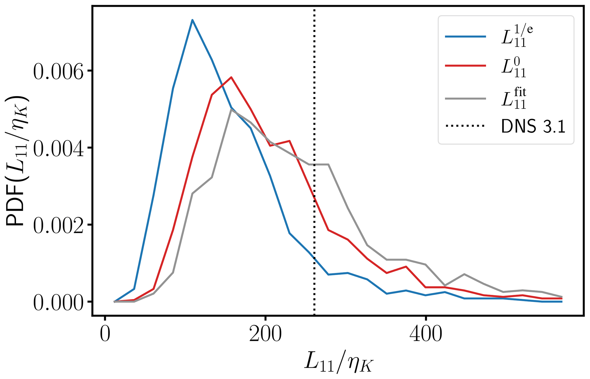
Figure A4 Different estimates of the integral length from DNS 3.1 with R_λ=302, I=1 %, θ=0^∘ and the maximal available averaging window. $L_{\mathrm{11}}^{\mathrm{0}}$ is inferred from integrating f(r) to its first zero, whereas $L_{\mathrm{11}}^{\mathrm{1}/\mathrm{e}}$ refers to the integration of $f\left(r\right)>\mathrm{1}/\mathrm{e}$. $L_{\mathrm{11}}^{\mathrm{fit}}$ extends f(r) with an exponential tail where the integration is performed up to infinity. The dotted black line is the reference from DNS 3.1 obtained by Eq. (11). All estimates are re-scaled by η_K.

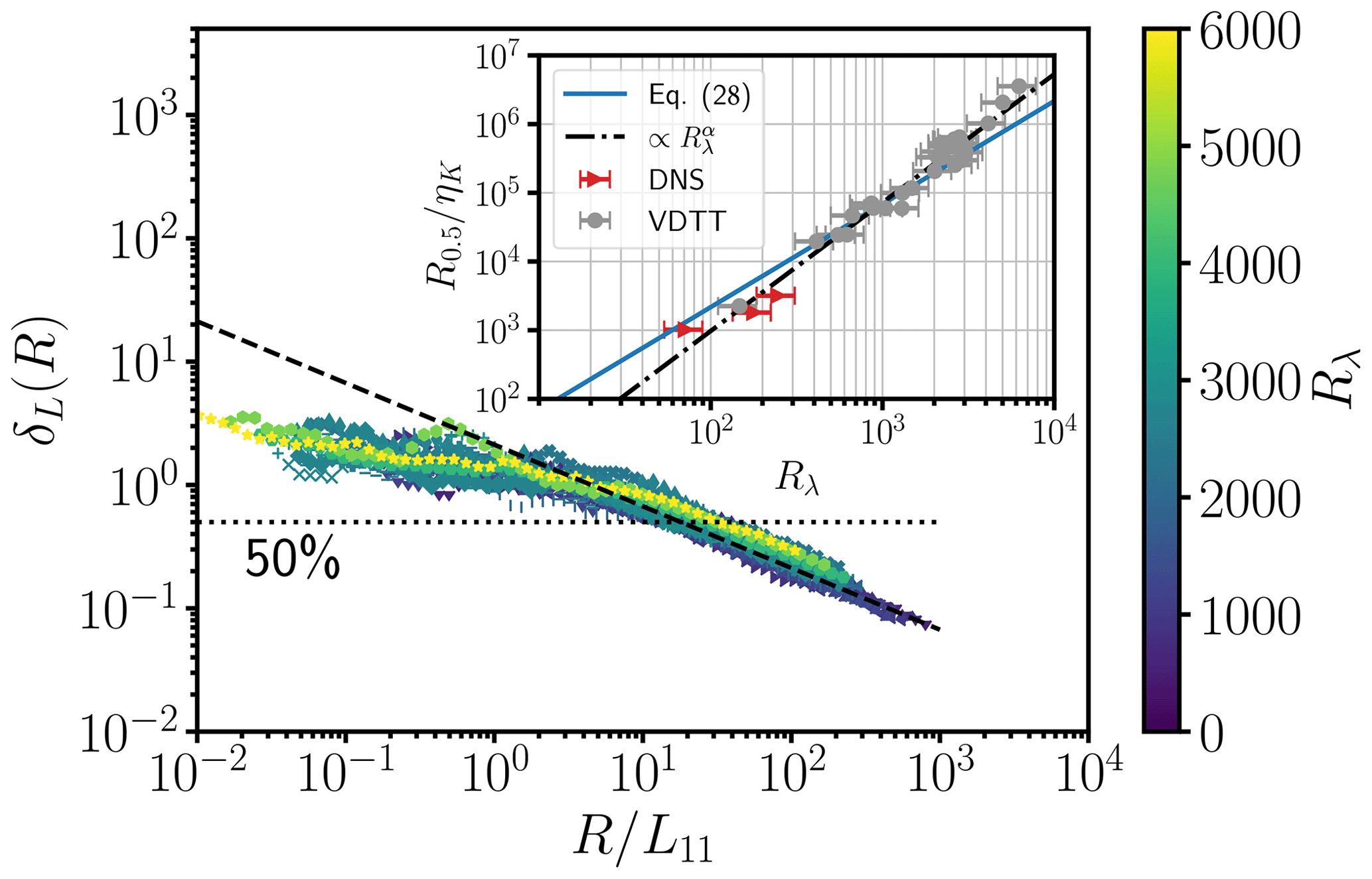
Figure A5 Convergence of energy dissipation rate estimates for ϵ_L. The empirical random error δ_L(R) is plotted as a function of the re-scaled averaging window size $R/L_{\mathrm{11}}$ from VDTT experiments at various R_λ values. The analytical result for the random error (Eq. 22) is shown by the dashed black line. Inset: the insets show the length of the averaging window in terms of η_K where δ_L(R) is less than 50 % as a function of the Taylor-microscale Reynolds number R_λ. The inset plot shows data from DNS 1.3, 2.3 and 3.3 (red triangles) and the VDTT (grey circle). The three red dots mark the experiments with the highest R_λ where the isotropy of the grid forcing in the VDTT is not guaranteed anymore. The solid blue line shows Eq. (28) resolved for $R_{\mathrm{0.5}}/{\mathit{\eta }}_K$. The double logarithmic fit ($\log R/{\mathit{\eta }}_K=\frac{\mathrm{3}}{\mathrm{4}}\log \frac{\mathrm{9}}{\mathrm{4}}\frac{\mathrm{3}}{\mathrm{20}}-\mathrm{2}\log a_{\mathrm{fit}}+\mathit{\alpha }\log R_{\mathit{\lambda }}$) is performed for the scaling argument, resulting in $\mathit{\alpha }=\mathrm{1.87}\pm \mathrm{0.06}$ and $a_{\mathrm{fit}}=\mathrm{1.75}\pm \mathrm{0.22}$ (dash-dotted black line).

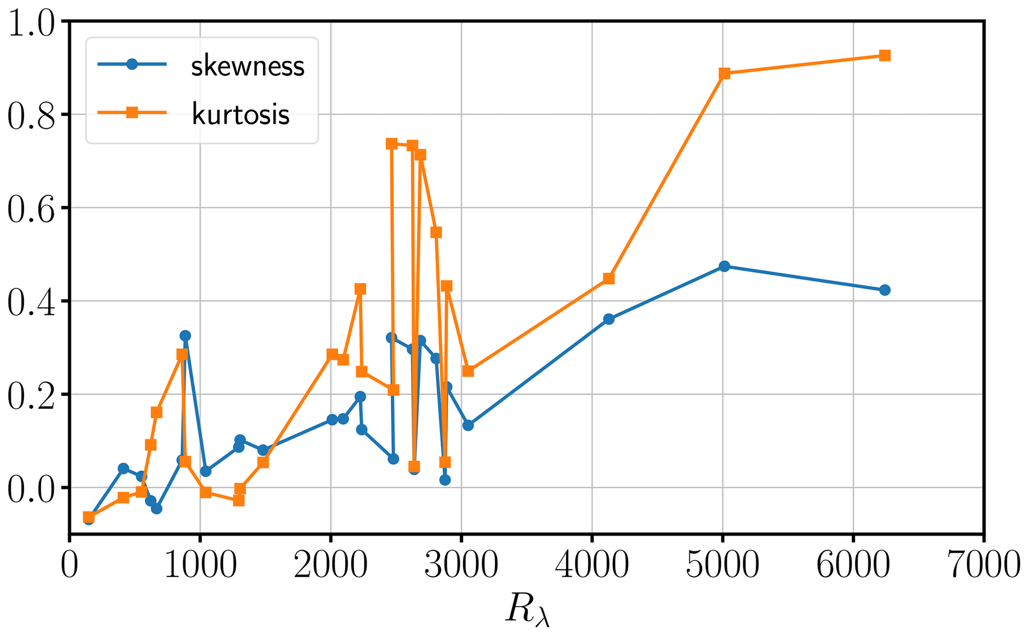
Figure A6 Skewness and kurtosis of all VDTT experiments as a function of R_λ. The skewness vanishes for normally distributed velocity time records. Similarly, the kurtosis equals zero for normally distributed velocity time records, according to Fisher's convention, which is a measure for the excess kurtosis.

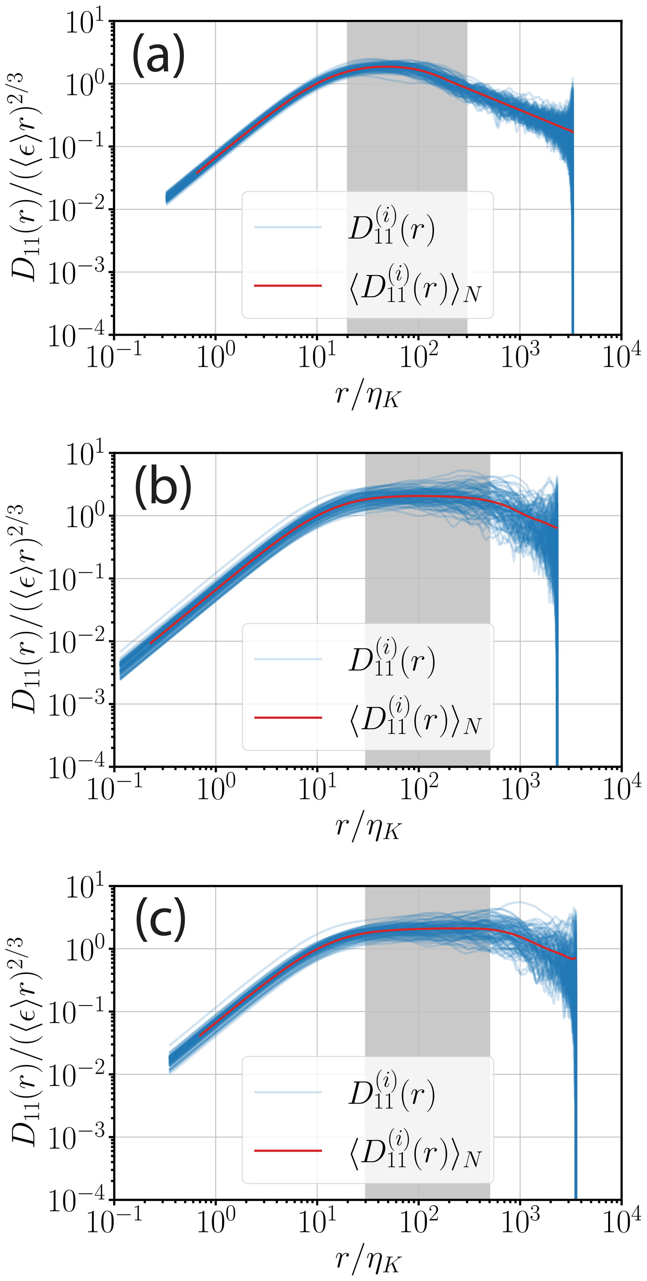
Figure A7 Compensated longitudinal second-order structure functions for DNS 1.1 (a), DNS 2.1 (b) and DNS 3.1 (c). The grey shaded region represents the fit range (Eq. 7) for each DNS. The individual longitudinal second-order structure functions are calculated from the velocity time records along the e₁ direction of each virtual probe (blue lines). The ensemble-averaged longitudinal second-order structure functions are shown in red.

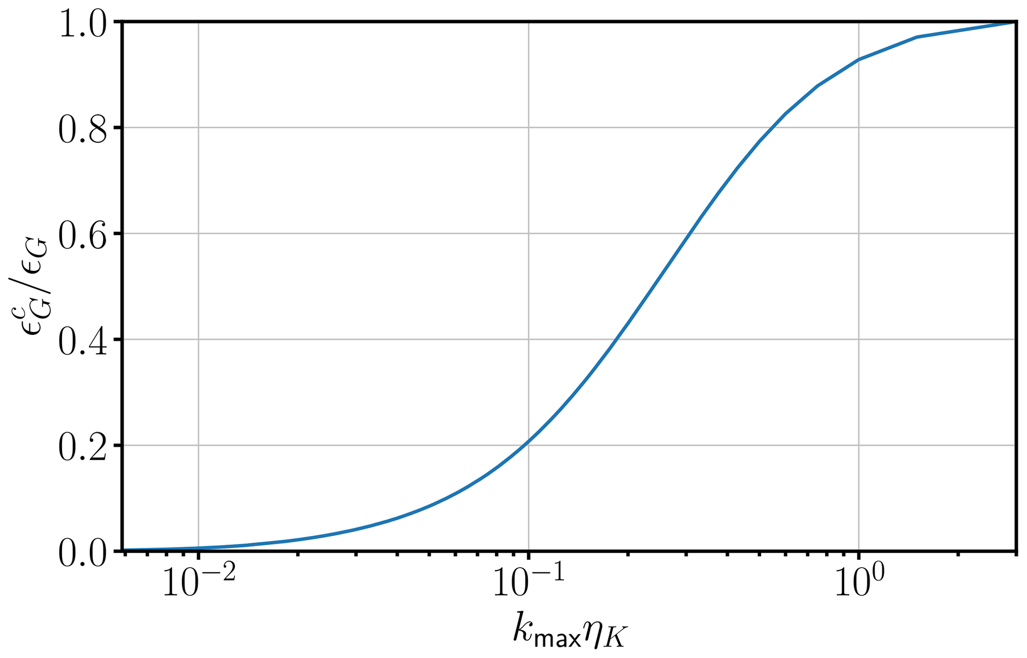
Figure A8 Resolution effect on ϵ_G. ${\mathit{ϵ}}_G^{\mathrm{c}}$ refers to the coarse-grained velocity time record. Coarse graining is realized by taking only every nth value of the fully resolved velocity time record where $n\in [\mathrm{1},\mathrm{512}]$, thereby controlling the resolution k_maxη_K. Velocity data are taken from DNS 2.0 (R_λ=142, R≈32 000η_K, I=10 %, θ=0^∘).

Appendix B: Impact of random-sweeping effects on the gradient method

In the following, we illustrate how one obtains an expression for the impact of random-sweeping effects on the dissipation rate estimate in terms of the turbulence intensity using the gradient method ${\mathit{ϵ}}_G=\langle \mathit{ϵ}\rangle [\mathrm{1}+\mathrm{5}{I}^{\mathrm{2}}]$ (Lumley, 1965; Wyngaard and Clifford, 1977). We consider a model wave-number–frequency spectrum (Wilczek and Narita, 2012; Wilczek et al., 2014), which is based on the same modeling assumptions used in Wyngaard and Clifford (1977). It enables us to conduct a systematic assessment of the interplay between Taylor's hypothesis and the random-sweeping effects. The model wave-number–frequency spectrum tensor Φ_ij(κ,ω) can be derived from an elementary linear random-advection model (Kraichnan, 1964; Wilczek and Narita, 2012; Wilczek et al., 2014), which in the case of SHI turbulence can be expressed in terms of the energy spectrum tensor Φ_ij(κ):

$$\begin{array}{}\text{(B1)}& {\mathrm{\Phi }}_{ij}(\mathit{\kappa },\mathit{\omega })={\displaystyle \frac{{\mathrm{\Phi }}_{ij}\left(\mathit{\kappa }\right)}{\sqrt{\mathrm{2}\mathit{\pi }{\mathit{\kappa }}^{\mathrm{2}}{I}^{\mathrm{2}}{U}^{\mathrm{2}}}}}\exp \left(-{\displaystyle \frac{(\mathit{\omega }/U-{\mathit{\kappa }}_{\mathrm{1}}{)}^{\mathrm{2}}}{\mathrm{2}{\mathit{\kappa }}^{\mathrm{2}}{I}^{\mathrm{2}}}}\right).\end{array}$$

Within the model, the wave-number–frequency spectrum Φ_ij(κ,ω) consists of the energy spectrum tensor in wavenumber space Φ_ij(κ) multiplied by a Gaussian frequency distribution. Φ_ij(κ,ω) has a mean value determined by ω=κ₁U, i.e., Taylor's hypothesis expressed in Fourier space, and a variance proportional to the turbulence intensity. When the turbulence intensity tends toward zero at a fixed mean velocity, the frequency distribution tends toward a delta function, re-establishing the one-to-one correspondence between the frequency and the wavenumber in the direction of the mean flow. To establish the connection to the different methods using longitudinal components and Taylor's hypothesis, we consider the $i=j=\mathrm{1}$ component of Eq. (B1). One obtains the estimate for the longitudinal wavenumber spectrum based on Taylor's hypothesis, which includes the effect of random sweeping, by first integrating over the wave vector space. This leads to the frequency spectrum, which corresponds to the one obtained from temporal single-point measurements of the longitudinal velocity component. Then, one applies Taylor's hypothesis, corresponding to the substitution ω=κ₁U, which leads to

$$\begin{array}{}\text{(B2)}& {\displaystyle }\mathrm{2}\left[\int {\mathrm{\Phi }}_{\mathrm{11}}({\mathit{\kappa }}^{\prime },\mathit{\omega })d{\mathit{\kappa }}^{\prime }\right]d\mathit{\omega }\stackrel{\mathit{\omega }={\mathit{\kappa }}_{\mathrm{1}}U}{=}{E}_{\mathrm{11}}\left({\mathit{\kappa }}_{\mathrm{1}}\right)d{\mathit{\kappa }}_{\mathrm{1}}.\end{array}$$

Finally, this enables us to evaluate the influence of random sweeping on the gradient method since it is closely related to the wavenumber spectrum. Expressed in wavenumber space, the relation (Eq. 6) takes the following form, where we insert Eqs. (B1)–(B2) and solve the corresponding Gaussian integral over ω in the second step:

$$\begin{array}{}\text{(B3)}& {\mathit{ϵ}}_G=\mathrm{15}\mathit{\nu }\int {\mathit{\kappa }}_{\mathrm{1}}^{\mathrm{2}}{E}_{\mathrm{11}}\left({\mathit{\kappa }}_{\mathrm{1}}\right)\mathrm{d}{\mathit{\kappa }}_{\mathrm{1}}=\langle \mathit{ϵ}\rangle [\mathrm{1}+\mathrm{5}{I}^{\mathrm{2}}].\end{array}$$

Hence, we recover, as expected, the result by Lumley (1965) and Wyngaard and Clifford (1977).

To numerically assess how random sweeping smears out the spectrum at finite turbulence intensities (see Fig. 4), we assumed a model wavenumber spectrum (Pope, 2000, Eq. 6.246 ff.):

$$\begin{array}{}\text{(B4)}& \begin{array}{rl}E\left(\mathit{\kappa }\right)=& C_K\langle \mathit{ϵ}{\rangle }^{\mathrm{2}/\mathrm{3}}{\mathit{\kappa }}^{-\mathrm{5}/\mathrm{3}}{\left({\displaystyle \frac{\mathit{\kappa }L}{{\left[(\mathit{\kappa }L{)}^{\mathrm{2}}+c_L\right]}^{\mathrm{1}/\mathrm{2}}}}\right)}^{\mathrm{5}/\mathrm{3}+p_{\mathrm{0}}}\\ & \exp \left(-\mathit{\beta }\mathit{\kappa }{\mathit{\eta }}_K\right),\end{array}\end{array}$$

where L is the energy injection scale and c_L=6.78, p₀=2 and β=2.094 are positive constants. Based on this model wavenumber spectrum, we first obtain E₁₁(κ) through Eq. (A7). One can then evaluate Eq. (B2), resulting in the spectrum being smeared out by random sweeping.

Appendix C: Effect of probe misalignment

Due to the misalignment, the probe frame of reference is rotated with respect to the frame given by the mean velocity. Without loss of generality, we assume that the misalignment is due to a rotation around the $\widehat{\mathit{n}}={\mathit{e}}_{\mathrm{3}}$ axis with the angle θ; see Fig. 5.

The misalignment has two consequences. First, the estimated mean velocity differs from the true mean velocity, which leads to errors when evaluating Taylor's hypothesis. Second, the measured velocity component is not the true velocity component but rather a combination of the longitudinal and transverse components.

In the probe frame of reference, we assume that we measure the longitudinal velocity field component, i.e., the component along the probe orientation ${\mathit{e}}_{\mathrm{1}}^{\prime }$. The mean of this component gives us the estimate of the mean velocity of the probe U^′. Due to the misalignment between probe and true mean velocity, we underestimate the mean velocity $U^{\prime }=U\cos \mathit{\theta }$ compared to the true mean velocity U. As we apply Taylor's hypothesis to convert temporal increments into spatial distances, we therefore also underestimate the spatial distances:

$$\begin{array}{}\text{(C1)}& \stackrel{\mathrm{̃}}{r}=U^{\prime }\mathrm{\Delta }t=\cos \mathit{\theta }U\mathrm{\Delta }t=\cos \mathit{\theta }r.\end{array}$$

Here $\stackrel{\mathrm{̃}}{r}$ denotes the estimated spatial distance and r the true distance that the probe moved.

The sampling direction of the probe, given by the direction of the mean velocity, e₁, can be expressed in the probe frame of reference:

$$\begin{array}{}\text{(C2)}& {\mathit{e}}_{\mathrm{1}}=\cos \mathit{\theta }{\mathit{e}}_{\mathrm{1}}^{\prime }-\sin \mathit{\theta }{\mathit{e}}_{\mathrm{2}}^{\prime }.\end{array}$$

Combining these two aspects, the vectorial distance covered by the probe in terms of the estimated one, therefore, becomes

$$\begin{array}{}\text{(C3)}& {\displaystyle }r{\mathit{e}}_{\mathrm{1}}={\displaystyle \frac{\stackrel{\mathrm{̃}}{r}}{\cos \mathit{\theta }}}(\cos \mathit{\theta }{\mathit{e}}_{\mathrm{1}}^{\prime }-\sin \mathit{\theta }{\mathit{e}}_{\mathrm{2}}^{\prime }).\end{array}$$

In the probe frame of reference, the covariance tensor is given by (see Eq. A1)

$$\begin{array}{}\text{(C4)}& {\displaystyle }{R}_{ij}^{\prime }\left({\mathit{r}}^{\prime }\right)=\langle {u^{\prime }}^{\mathrm{2}}\rangle \left(g\left(r^{\prime }\right){\mathit{\delta }}_{ij}+\left[f\left(r^{\prime }\right)-g\left(r^{\prime }\right)\right]{\displaystyle \frac{r_i^{\prime }{r}_j^{\prime }}{{r^{\prime }}^{\mathrm{2}}}}\right).\end{array}$$

By application of Taylor's hypothesis, we can evaluate this tensor at ${\mathit{r}}^{\prime }=\stackrel{\mathrm{̃}}{r}/\cos \mathit{\theta }(\cos \mathit{\theta }{\mathit{e}}_{\mathrm{1}}^{\prime }+\sin \mathit{\theta }{\mathit{e}}_{\mathrm{2}}^{\prime })$. So the corresponding longitudinal component $i=j=\mathrm{1}$ in terms of the estimated distance $\stackrel{\mathrm{̃}}{r}$ becomes

$$\begin{array}{}\text{(C5)}& \begin{array}{rl}{R}_{\mathrm{11}}^{\prime }& \left({\mathit{r}}^{\prime }\right(\stackrel{\mathrm{̃}}{r}\left)\right)/\langle {u^{\prime }}^{\mathrm{2}}\rangle =g(\stackrel{\mathrm{̃}}{r}/\cos \mathit{\theta })+\left[f(\stackrel{\mathrm{̃}}{r}/\cos \mathit{\theta })\right.\\ & \left.-g(\stackrel{\mathrm{̃}}{r}/\cos \mathit{\theta })\right]{\cos }^{\mathrm{2}}\mathit{\theta },\end{array}\end{array}$$

which, due to the misalignment, we interpret as the measured autocorrelation function. Then, the measured longitudinal integral length scale, Eq. (11), amounts to

$$\begin{array}{}\text{(C6)}& \begin{array}{rl}{L}_{\mathrm{11}}^{\prime }\left(\mathit{\theta }\right)=& \underset{\mathrm{0}}{\overset{\mathrm{\infty }}{\int }}d\stackrel{\mathrm{̃}}{r}{R}_{\mathrm{11}}^{\prime }\left({\mathit{r}}^{\prime }\right(\stackrel{\mathrm{̃}}{r}\left)\right)/\langle {u^{\prime }}^{\mathrm{2}}\rangle \\ =& \underset{\mathrm{0}}{\overset{\mathrm{\infty }}{\int }}dr\cos \mathit{\theta }\left({\cos }^{\mathrm{2}}\mathit{\theta }f\right(r)+(\mathrm{1}-{\cos }^{\mathrm{2}}\mathit{\theta }\left)g\right(r\left)\right)\\ =& {\displaystyle \frac{\mathrm{1}}{\mathrm{2}}}{L}_{\mathrm{11}}\cos \mathit{\theta }\left(\mathrm{1}+{\cos }^{\mathrm{2}}\mathit{\theta }\right),\end{array}\end{array}$$

where the integration of f(r) and g(r) is carried out in the last step (see Eq. 11) while considering the fact that $L_{\mathrm{22}}=L_{\mathrm{11}}/\mathrm{2}$ for isotropic turbulence (Pope, 2000). Therefore, the energy injection scale estimate of the dissipation rate, Eq. (10), overestimates the dissipation rate due to misalignment as follows:

$$\begin{array}{}\text{(C7)}& {\displaystyle }{\mathit{ϵ}}_L\left(\mathit{\theta }\right)=C_{\mathit{ϵ}}{\displaystyle \frac{{\mathit{\sigma }}_{u_{\mathrm{1}}^{\prime }}^{\mathrm{3}}}{L_{\mathrm{11}}^{\prime }}}={\displaystyle \frac{\mathrm{2}}{\cos \mathit{\theta }\left(\mathrm{1}+{\cos }^{\mathrm{2}}\mathit{\theta }\right)}}{\mathit{ϵ}}_L\left(\mathrm{0}\right).\end{array}$$

The same arguments that we applied to the covariance tensor, of course, also hold for the second-order structure function tensor, Eq. (A2). Due to the effects of misalignment, it takes the form

$$\begin{array}{}\text{(C8)}& \begin{array}{rl}{D}_{\mathrm{11}}\left({\mathit{r}}^{\prime }\right(\stackrel{\mathrm{̃}}{r}\left)\right)& =D_{\mathrm{NN}}(\stackrel{\mathrm{̃}}{r}/\cos \mathit{\theta })+\left[D_{\mathrm{LL}}(\stackrel{\mathrm{̃}}{r}/\cos \mathit{\theta })\right.\\ & \left.-D_{\mathrm{NN}}(\stackrel{\mathrm{̃}}{r}/\cos \mathit{\theta })\right]{\cos }^{\mathrm{2}}\mathit{\theta }\\ & =D_{\mathrm{LL}}(\stackrel{\mathrm{̃}}{r}/\cos \mathit{\theta })\left({\displaystyle \frac{\mathrm{4}-{\cos }^{\mathrm{2}}\mathit{\theta }}{\mathrm{3}}}\right),\end{array}\end{array}$$

where in the inertial range of SHI turbulence the transverse second-order structure function $D_{\mathrm{NN}}\left(r\right)=D_{\mathrm{22}}\left(r\right)=D_{\mathrm{33}}\left(r\right)$ can be expressed as $D_{\mathrm{NN}}\left(r\right)=\mathrm{4}{D}_{\mathrm{LL}}\left(r\right)/\mathrm{3}=\mathrm{4}{C}_{\mathrm{2}}(r\mathit{ϵ}{)}^{\mathrm{2}/\mathrm{3}}/\mathrm{3}$ (Pope, 2000). Therefore, the estimated dissipation rate using the second-order SF method (cf. Eq. 7) is affected by misalignment as

$$\begin{array}{}\text{(C9)}& \begin{array}{rl}{\mathit{ϵ}}_{I\mathrm{2}}\left(\mathit{\theta }\right)& ={\left({\displaystyle \frac{D_{\mathrm{11}}\left({\mathit{r}}^{\prime }\right(\stackrel{\mathrm{̃}}{r}\left)\right)}{C_{\mathrm{2}}}}\right)}^{\mathrm{3}/\mathrm{2}}{\displaystyle \frac{\mathrm{1}}{\stackrel{\mathrm{̃}}{r}}}\\ & ={\displaystyle \frac{\mathrm{1}}{\cos \mathit{\theta }}}{\left({\displaystyle \frac{\mathrm{4}-{\cos }^{\mathrm{2}}\mathit{\theta }}{\mathrm{3}}}\right)}^{\mathrm{3}/\mathrm{2}}{\mathit{ϵ}}_{I\mathrm{2}}\left(\mathrm{0}\right).\end{array}\end{array}$$

The misalignment error for the gradient method can be estimated analytically starting from the longitudinal component of the velocity gradient covariance tensor $R_{\mathrm{1111}}^{\prime }$, Eq. (A4). Following similar arguments as above and starting from Eq. (A4), we obtain

$$\begin{array}{}\text{(C10)}& \begin{array}{rl}& R_{\mathrm{1111}}^{\prime }\left(\mathbf{0}\right)=-\underset{r^{\prime }\to \mathrm{0}}{lim}{\partial }_{r_{\mathrm{1}}^{\prime }}^{\mathrm{2}}{R}_{\mathrm{11}}^{\prime }\left({\mathit{r}}^{\prime }\right)=-\underset{\stackrel{\mathrm{̃}}{r}\to \mathrm{0}}{lim}{\partial }_{\stackrel{\mathrm{̃}}{r}}^{\mathrm{2}}{R}_{\mathrm{11}}^{\prime }\left({\mathit{r}}^{\prime }\right(\stackrel{\mathrm{̃}}{r}\left)\right)\\ & =-{\displaystyle \frac{\langle {u^{\prime }}^{\mathrm{2}}\rangle }{{\cos }^{\mathrm{2}}\mathit{\theta }}}\underset{r\to \mathrm{0}}{lim}{\partial }_r^{\mathrm{2}}\left[g\left(r\right)+\left[f\right(r)-g(r\left)\right]{\displaystyle \frac{r^{\mathrm{2}}{\cos }^{\mathrm{2}}\mathit{\theta }}{r^{\mathrm{2}}}}\right],\end{array}\end{array}$$

where we expressed the estimated distance through the true one $\stackrel{\mathrm{̃}}{r}=r\cos \mathit{\theta }$ in the second line. Using ${\partial }_r^{\mathrm{2}}g\left(r\right)=\mathrm{2}{\partial }_r^{\mathrm{2}}f\left(r\right)+\frac{r}{\mathrm{2}}{\partial }_r^{\mathrm{3}}f\left(r\right)$ (Pope, 2000), the velocity gradient covariance tensor reduces to

$$\begin{array}{}\text{(C11)}& \begin{array}{rl}{R}_{\mathrm{1111}}^{\prime }\left(\mathbf{0}\right)& =-{\displaystyle \frac{\langle {u^{\prime }}^{\mathrm{2}}\rangle }{{\cos }^{\mathrm{2}}\mathit{\theta }}}\underset{r\to \mathrm{0}}{lim}\left[(\mathrm{2}-{\cos }^{\mathrm{2}}\mathit{\theta }){\partial }_r^{\mathrm{2}}f\left(r\right)\right.\\ & \left.+(\mathrm{1}-{\cos }^{\mathrm{2}}\mathit{\theta }){\displaystyle \frac{r}{\mathrm{2}}}{\partial }_r^{\mathrm{3}}f\left(r\right)\right]\\ & =〈{\left({\displaystyle \frac{\partial u}{\partial x_{\mathrm{1}}}}\right)}^{\mathrm{2}}〉{\displaystyle \frac{\mathrm{2}-{\cos }^{\mathrm{2}}\mathit{\theta }}{{\cos }^{\mathrm{2}}\mathit{\theta }}},\end{array}\end{array}$$

where $-\langle {u^{\prime }}^{\mathrm{2}}\rangle {lim}_{r\to \mathrm{0}}{\partial }_r^{\mathrm{2}}f\left(r\right)=\langle (\partial u/\partial x_{\mathrm{1}}{)}^{\mathrm{2}}\rangle$ (Pope, 2000) is used for the last step. The energy dissipation rate based on the gradient method, Eq. (6), is overestimated by the very same factor due to misalignment:

$$\begin{array}{}\text{(C12)}& {\displaystyle }{\mathit{ϵ}}_G\left(\mathit{\theta }\right)={\displaystyle \frac{\mathrm{2}-{\cos }^{\mathrm{2}}\mathit{\theta }}{{\cos }^{\mathrm{2}}\mathit{\theta }}}{\mathit{ϵ}}_G\left(\mathrm{0}\right).\end{array}$$