the Creative Commons Attribution 4.0 License.
the Creative Commons Attribution 4.0 License.
 | 09 Jan 2024
New insights from the Jülich Ozone Sonde Intercomparison Experiment: calibration functions traceable to one ozone reference instrument
Deniz Poyraz
Roeland Van Malderen
Anne M. Thompson
David W. Tarasick
Ryan M. Stauffer
Bryan J. Johnson
Debra E. Kollonige
Although in principle ECC (electrochemical concentration cell) ozonesondes are absolute measuring devices, in practice they have several “artefacts” which change over the course of a flight. Most of the artefacts have been corrected in the recommendations of the Assessment of Standard Operating Procedures for Ozone Sondes (ASOPOS) report (Smit et al., 2021), giving an overall uncertainty of 5 %–10 % throughout the profile. However, the conversion of the measured cell current into the sampled ozone concentration still needs to be quantified better, using time-varying background current and more appropriate pump efficiencies. We describe an updated methodology for ECC sonde data processing that is based on the Jülich Ozone Sonde Intercomparison Experiment (JOSIE) 2009/2010 and JOSIE Southern Hemisphere Additional Ozonesondes (JOSIE-SHADOZ) 2017 test chamber data. The methodology resolves the slow and fast time responses of the ECC ozonesonde and in addition applies calibration functions to make the sonde data traceable to the JOSIE ozone reference UV photometer (OPM). The stoichiometry () factors and their uncertainties along with fast and slow reaction pathways for the different sensing solution types used in the global ozonesonde network are determined. Experimental evidence is given for treating the background current of the ECC sensor as the superposition of a constant ozone-independent component (IB0, measured before ozone exposure in the sonde preparation protocol) and a slow time-variant ozone-dependent current determined from the initial measured ozone current using a first-order numerical convolution. The fast sensor current is refined using the time response determined in sonde preparation with a first-order deconvolution scheme. Practical procedures for initializing the numerical deconvolution and convolution schemes to determine the slow and fast ECC currents are given. Calibration functions for specific ozonesondes and sensing solution type combinations were determined by comparing JOSIE 2009/2010 and JOSIE-SHADOZ 2017 profiles with the JOSIE OPM. With fast and slow currents resolved and the new calibration functions, a full uncertainty budget is obtained. The time response correction methodology makes every ozonesonde record traceable to one standard, i.e. the OPM of JOSIE, enabling the goal of a 5 % relative uncertainty to be met throughout the global ozone network.
- Article
(15304 KB) - Full-text XML
-
Supplement
(10898 KB) - BibTeX
- EndNote


Although it is a minor trace gas constituent of the Earth's atmosphere, ozone plays several essential roles in its chemistry and physics. In the stratosphere, where about 90 % of the total ozone amount resides, ozone protects life on Earth by absorbing the harmful ultraviolet (UV) radiation from the sun, adding heat to the stratosphere. In the upper troposphere, ozone is an important absorber of infrared radiation, acting as a powerful greenhouse gas (IPCC-Climate Change, 2013, 2023). Ozone is the primary source of the hydroxyl (OH) radical in the troposphere, controlling the lifetime of hundreds of pollutants (Seinfeld and Pandis, 2016) and determining the oxidizing capacity of the atmosphere (Thompson, 1992). The stratosphere is a natural source of tropospheric ozone, but approximately half of the ozone in the troposphere is formed photochemically when combustion (vehicular, industrial or pyrogenic) processes release NOx (), carbon monoxide (CO) and hydrocarbons (also referred to as volatile organic compounds (VOCs)) that react through free-radical cycles in the presence of UV. VOCs may also originate from combustion or natural sources, the latter predominantly from vegetation and to a lesser extent from the ocean. Surface ozone is considered a pollutant with adverse impacts on human and animal health (e.g. respiratory problems) and on vegetation (Mills et al., 2018) and is a primary marker for “air quality,” setting the scale for good, fair and unhealthy definitions used by local air quality agencies (Garner and Thompson, 2013). The photochemistry of ozone pollution or “smog” was first identified by Haagen-Smit (1952) in the early 1950s and was found to typically occur at very high concentrations of VOCs and NOx, whereby organic particles also play an important role (e.g. Seinfeld and Pandis, 2016); surface ozone measurements became widespread as regions or nations enacted regulations to mitigate episodes of high ozone.
Measurements of stratospheric ozone gained attention in the 1960s and 1970s when it was recognized that natural levels of ozone were regulated by catalytic cycles involving nitrogen oxides (NOx, N2O5, NO3 and HNO3), hydrogen oxides (with H2O vapour a source of OH and HO2; ) and halogens (XO and XO2, where X is Cl or Br derived from oceanic methyl chloride and methyl bromide). Anthropogenic perturbations of these cycles were investigated when it was recognized that emissions of N- and Cl-containing compounds by rockets and high-altitude aircraft could threaten stratospheric ozone (Crutzen, 1970; Stolarski and Cicerone, 1974). A worse threat was hypothesized when it was realized that chlorofluorocarbons (CFCs) present in the atmosphere (Lovelock et al., 1973) that were relatively inert in the troposphere could enter the stratosphere and destroy ozone photochemically there (Molina and Rowland, 1974). Perturbed stratospheric ozone chemistry by CFCs was a cause for alarm, leading to the first regulations in CFC usage in the 1970s. However, it was not until ground-based total ozone monitoring (Farman et al., 1985) discovered catastrophic springtime ozone loss over Antarctica in 1984–1985 that international action was taken to phase out ozone-depleting substances through the 1987 signing of the Montreal Protocol (UNEP-Ozone Secretariat, 2020). Implementation of the Montreal Protocol and its follow-on amendments requires governments to monitor ozone, reporting every 4 years to the World Meteorological Organization (WMO) and United Nations Environment Programme (UNEP) in scientific assessments on the global vertical distribution of ozone and its long-term changes. Since 1991 there have been nine WMO/UNEP scientific assessments, with the most recent report released in 2022 (WMO/UNEP, 2023).
Global monitoring of total ozone has relied on satellite instruments since the 1970s, but ground-based instrumentation deployed on all continents still provides ground truth. In particular, ozonesondes are essential for satellite algorithms and validation of satellite-derived profiles and reanalysis products (Wang et al., 2020; Thompson et al., 2021, 2022). Balloon-borne ozonesondes, flown together with radiosondes, make relatively inexpensive, accurate, all-weather measurements of the ozone concentrations from the ground to 30 km or higher, with ∼100 m vertical resolution (Smit, 2014). The electrochemical concentration cell (ECC) ozonesonde has been deployed for more than 50 years with approximately 60 stations currently launching ozonesondes on all continents (global ozonesonde network shown in Figs. 1 and 2 in Smit et al., 2021; Thompson et al., 2022; Stauffer et al., 2022). Ozonesonde data constitute the most important record for deriving ozone trends throughout both the stratosphere and the troposphere, particularly in the climate-sensitive altitude region near the tropopause where satellite measurements are most uncertain. Strategic ozonesonde networks like Match and IONS (Intensive Ozonesonde Network Study) have been organized to support aircraft campaigns in characterizing photochemical and dynamical interactions affecting vertical and regional ozone distributions (Thompson et al., 2007a, 2011; Tarasick et al., 2010).
1.1 Establishing quality assurance/quality control (QA/QC) practices for ozonesondes (1996–2021)
Despite the advantages of ozonesonde profiles, there is a challenge in that each ozonesonde instrument is unique, is typically launched only once and must be carefully prepared prior to launch in order to obtain accurate data. Processing of the final measurement is carried out using certain parameters determined pre-launch. In addition, there are two manufacturers of ozonesondes that show systematic offsets relative to each other. Further biases in ozonesonde datasets can occur because three variants of the sensing solution that produce the ECC current signal from the ozone are currently in use. The ozonesonde community has created guidelines for operations and data processing applicable to the range of instrument and sensing solution types used in the global ECC sonde network. When the guidelines are followed, it is possible for consistently high-quality data to be collected across the global network.
The creation of guidelines or “best practices” has evolved over the past 20 years in a process referred to as the Assessment of Standard Operating Procedures (SOPs) for Ozone Sondes (ASOPOS) and organized through the WMO Global Atmosphere Watch (GAW). The key element of ASOPOS was the establishment of the World Calibration Centre for Ozone Sondes (WCCOS) with a custom-designed Environmental Simulation Facility (ESF) at the Forschungszentrum in Jülich, Germany, in 1995 (GAW Report No. 104, 1994; Smit et al., 2000). The ESF consists of an absolute ozone measuring reference; a fast response (2 s); and an accurate (2 %–3 %), dual-beam UV-absorption ozone photometer (OPM) (Proffitt and McLaughlin, 1983) attached to the chamber that enables control of pressure, temperature and ozone concentration simulating flight conditions of an ozone sounding at up to 35 km over ∼2 h (Smit et al., 2007). Up to four ozonesonde instruments at once can be intercompared through this process. Simulations in the ESF included conditions of polar, mid-latitude, subtropical and tropical sonde launches. Other aspects of sonde operations, e.g. response times to rapid changes in ozone concentration, are also tested in the ESF. Since 1996, nine Jülich Ozone Sonde Intercomparison Experiment (JOSIE) campaigns have been conducted at WCCOS and documented in a series of publications for JOSIE 1996 (Smit and Kley, 1998), JOSIE 1998 (Smit and Sträter, 2004a), JOSIE 2000 (GAW Report No. 158; Smit and Sträter, 2004b; Smit et al., 2007; Thompson et al., 2007b), JOSIE 2009/2010 and JOSIE 2017 (Thompson et al., 2019). The first three JOSIE campaigns, which tested several non-ECC instruments as well as Science Pump Corporation (SPC) and Environmental Science (EN-SCI) ECC instruments, showed the ECC sonde to be more accurate. After JOSIE 2000 only ECC sondes were tested in WCCOS.
In 2004 the WMO BESOS (Balloon Experiment on Standards for Ozonesondes) field campaign, carried out in Laramie (Wyoming, USA), deployed a large gondola with 18 ozonesondes and the OPM of WCCOS (Deshler et al., 2008) with results similar to those of JOSIE 2000. These early experiments demonstrated that high precision and accuracy depend not only on the sonde manufacturer and sensing solution strength, but also on pre-launch preparation details. Smit et al. (2007) concluded that standardization of operating procedures for ECC sondes yields a precision better than ± (3 %–5 %) and an accuracy of about ± (5 %–10 %) for up to 30 km altitude.
In 2004 an expert team of ozonesonde operators, data providers and manufacturers formally instituted ASOPOS to analyse the results of BESOS and the JOSIE campaigns up to that time. The ASOPOS goal was to ensure consistency of data quality across stations and within individual station time series by specifying how to prepare and operate the ozonesonde instrument and to accurately process and report profile data. The first set of SOPs recommended by ASOPOS, based on the JOSIE campaigns from 1996 to 2000 and BESOS, was published online in 2012 and as GAW Report No. 201 in 2014 (Smit and the ASOPOS Panel, 2014). To make (historical) ozonesonde time series records compliant with the ASOPOS standards, an OzoneSonde Data Quality Assessment (O3S-DQA) activity was initiated in 2011 within the framework of SI2N,1 resulting in procedures for “homogenizing” data and estimating uncertainties (Smit and O3S-DQA Panel, 2012; https://www.wccos-josie.org/en/o3s-dqa, last access: 10 December 2023); transfer functions in support of the guidelines were documented in Deshler et al. (2017). Within several years, roughly half of the global network stations had reprocessed their data (Tarasick et al., 2016; Van Malderen et al., 2016; Thompson et al., 2017; Sterling et al., 2018; Witte et al., 2017, 2018, 2019; Ancellet et al., 2022). Comparisons between original and homogenized data allowed elimination of significant systematic errors, particularly where changes in technique and/or equipment had been made.
The homogenized time series were based on having raw currents from the ozonesonde cells, a prerequisite for the analysis and processing methods of the present paper. However, the ozonesonde community agreed that several issues were unresolved. These included the complexity of the so-called “background current” characterized during the preparation and the lack of traceability of the archived ozone profile to an absolute standard. A JOSIE 2017 campaign was designed to address these concerns. In addition to the tests of prior JOSIE campaigns, the 2017 tests focused on a single regime, tropical profiles, to gather a larger set of statistics. A special challenge of tropical soundings is that near the tropopause the ozone concentrations can be very low such that the signal-to-noise ratio is very small (Thompson et al., 2007b), causing large relative uncertainties in the ozonesonde readings (Smit et al., 2007). JOSIE 2017 (also called JOSIE-SHADOZ) was carried out with eight SHADOZ operators, who supplied their home-prepared sensing solutions following their own preparation procedures for half the simulations (Thompson et al., 2019). The other half of the simulations tested a lower-buffer variant of the sensing solution with the WMO GAW SOPs. The overall results of JOSIE 2017 resembled those of the 1996–2000 JOSIE and BESOS campaigns. In other words, the offsets of the various instruments–sensing solution types (SSTs) from the OPM reference and associated biases of ECC sonde instruments and SSTs had not changed over more than 20 years.
The ASOPOS 2.0 Panel formed in 2018 to review the JOSIE 2017 campaign data along with lessons learned from reprocessed datasets and the JOSIE 2009/2010 results. ASOPOS 2.0 published GAW Report No. 268, “Ozonesonde Measurement Principles and Best Operational Practices” (Smit et al., 2021), as an update to Smit and the ASOPOS Panel (2014). The newer report gives the same recommendations as Smit and the ASOPOS Panel (2014) on sonde manufacturer–SST combinations but stricter and more unified SOPs. The latter consist of more detailed recommendations based on physical principles of the ozonesonde measurement. More explicit procedures are given for data quality indicators, hardware usage, and maintenance and metadata. Smit et al. (2021) also specified for the first time how to report ozone profiles traceable to the standard OPM. However, the issues of a time-varying background current and the specification of uncertainties in the ozone measurement (and related pump efficiencies) required analysis beyond Smit et al. (2021) before consensus could be reached on data-processing recommendations. That is the scope of this paper.
1.2 Addressing residual ozonesonde QA/QC issues from Smit et al. (2021): outline of paper
Chapter 3 of Smit et al. (2021) draws on the Tarasick et al. (2021) review of ozonesonde performance characteristics. Both documents point out that the greatest barriers to reducing uncertainties in the final ozone measurement derive from (1) the use of improper pump efficiencies and (2) a background current that varies with ozone exposure (hence with time) over the course of the balloon ascent. The current paper revisits fundamentals of the ozonesonde measurement to overcome these two shortcomings. The methodology reported here to resolve the fast and slow time responses builds on an earlier study by Imai et al. (2013) and on the more recent work by Tarasick et al. (2021) and Vömel et al. (2020). We first give a more detailed description of the physical and chemical origin of the ECC ozonesonde signal (Sect. 2), illustrated with laboratory measurements from the Uccle, Belgium, ozonesonde station. Section 3 first corrects for the background signal composed of (i) a constant physical component (IB0) and (ii) a small and slowly varying (time constant 25 min) chemical component that varies with ozone exposure. The remaining fast component of the signal is then corrected by deconvolution with an exponential decay with a time constant between 20 and 30 s. Although the approach is similar to Vömel et al. (2020), an advantage of our updated method is that it is developed from and applied to dedicated JOSIE chamber data (JOSIE 2009/2010) that used consistently prepared ozonesondes, with detailed in-flight and post-flight measurements and metadata. Second, the simultaneous OPM measurements in the simulation chamber serve as reference data for determining key parameters of the method, e.g. the contribution of the slow component to the overall signal. In Sect. 4, the OPM reference data are used to evaluate the updated method with comparisons to the conventional method. For these analyses, measurements from all JOSIE campaigns, covering a range of simulated environments, are used. Comparing residuals of the corrected ozonesonde profiles to the OPM profiles allows us to determine a set of the calibration functions for each instrument–SST combination (Sect. 5) and to estimate uncertainties in the updated time response correction (TRC) method (Sect. 6). The TRC method is implemented with actual sounding data in Sect. 7 for ascent and descent profiles at tropical, mid-latitude and polar (Antarctic) stations, and improvements with respect to the conventional approach are quantified. A summary and outlook appear in Sect. 8.
2.1 Principle of operation
The ECC (electrochemical concentration cell) ozonesonde, developed by Komhyr (1969), uses an electrochemical method to measure ozone which is based on the titration of ozone in a neutral buffered potassium iodide (NBKI) sensing solution according to the redox reaction, Reaction (R1):
A neutral pH of ∼7 is obtained through the addition of a phosphate buffer (NaH2PO4⋅H2O and Na2HPO4⋅12H2O).
The titration involves a coulometric method employing electrochemical cells to determine the amount of generated “free” iodine (I2) per unit time through conversion into an electrical current at a depolarizing cathode electrode. The actual ECC component of the ozone sensor, made of Teflon or moulded plastic, consists of two chambers. Each chamber contains a platinum (Pt) mesh electrode that serves as cathode or anode. The chambers are immersed in a KI solution of different concentrations and linked together to provide an ion pathway and to prevent mixing of the cathode and anode concentrations.
Continuous operation is achieved by a small nonreactive gas sampling pump (Komhyr, 1967) forcing ozone in ambient air through the cathode cell that contains a lower-concentration KI sensing solution, causing an increase in free iodine (I2) according to the redox reaction, Reaction (R1). Transported by the stirring action of the air bubbles, the free I2 contacts the Pt cathode and is converted to 2 I− through the uptake of two electrons. At the Pt-anode surface, I− is converted to I2 through the release of two electrons. The overall cell reaction is
The electrical current IM (µA) generated in the external circuit of the electrochemical cell is directly related to the uptake rate of ozone in the sensing solution. By knowing the gas volume flow rate ΦP0 (cm3 s−1) of the air sampling pump and its temperature TP (K), the electrical cell current IM (µA), after subtracting a background current IB (µA), is converted to the ozone partial pressure (in mPa) (Komhyr, 1969):
The constant 0.043085 is determined by the ratio of the universal gas constant, R, to twice the Faraday constant, F (because two electrons flow in the electrical circuit from Reaction R2) (Komhyr, 1969).
The overall efficiency of conversion consists of the following.
- a.
Pump efficiency, ηP. This declines at lower pressures: at reduced air pressures (<100 hPa), the pump efficiency declines due to pump leakage, dead volume in the piston of the pump and the back pressure exerted on the pump by the cathode cell (Komhyr, 1967; Steinbrecht et al., 1998; Nakano and Morofuji, 2023).
- b.
Absorption (i.e. capture) efficiency, ηA. This is the efficiency for the transfer of the sampled gaseous ozone into the liquid phase. Although evaporation reduces the amount of the sensing solution available for ozone uptake, ηA is not significantly affected (Komhyr and Harris, 1971). This was confirmed by Davies et al. (2003), who determined experimentally at different pressures in a vacuum tank the absorption efficiency ηA from the responses of two ECC sondes connected in series. Thus, ηA remains at 1.0, with an uncertainty of % (Tarasick et al., 2021; Davies et al., 2003).
- c.
Conversion efficiency, ηC. This is the efficiency of the absorbed ozone in the cathode solution creating iodine that leads to the measured cell current IM. Historically, it has been assumed that ηC is unity at neutral pH (Saltzman and Gilbert, 1959; Komhyr, 1969, 1986). However, there is now a great deal of evidence that this is not quite the case, as will be discussed below.
Currently, there are two manufacturers of ECC ozonesondes, Science Pump Corporation and Environmental Science Corporation, most recently producing the SPC-6A and EN-SCI-Z ozonesonde series, respectively. The designs of both ECC types are similar, but differences include (i) the material of the electrochemical cell (Teflon for SPC-6A and moulded plastic for EN-SCI-Z), (ii) ion bridges (details are not known due to manufacturer proprietary issues) and (iii) the layout of the metal frame. Since 2014, a modified ECC-type ozonesonde manufactured at the Institute of Atmospheric Physics (IAP), Beijing, has been produced (Zhang et al., 2014a, b), but to date, few comparisons of the Chinese instrument with the well-characterized SPC-6A and EN-SCI models have been carried out. Thus, profiles from Chinese instruments are not included in the current study.
Three different aqueous sensing solution types (SSTs) are commonly used in the ECC sonde cathode cells: (i) SST1.0, 1.0 % KI and full buffer; (ii) SST0.5, 0.5 % KI and half buffer; and (iii) SST0.1, 1.0 % KI and th buffer (Smit et al., 2021). In all cases a KI-saturated cathode solution is employed in the anode cell. Laboratory studies by Johnson et al. (2002) found that, depending on the concentration of the cathode sensing solution, the stoichiometric ratio of the ozone to iodine conversion reaction, Reaction (R1), can increase from 1.00 up to 1.05–1.20. Johnson et al. (2002) determined that this increase is caused primarily by the phosphate buffer and to a lesser extent depends on the KI concentration. No significant influence of KBr concentration was observed, although its role is not well understood. From JOSIE 2000 (Smit et al., 2007), BESOS 2004 (Deshler et al., 2008) and multiple other sounding tests (e.g. Deshler et al., 2017), it is known that there is a significant difference in the ozone readings when sondes of the same type are operated with different sensing solutions, e.g. STT0.5 and SST1.0. Both sonde types exhibit a systematic change in sensitivity, about 5 %–10 % over the entire profile, when the sensing solution is changed from SST0.5 to SST1.0. Johnson et al. (2002) demonstrated that this offset is mostly caused by the phosphate buffer with a minor contribution from the KI concentration. In addition, the EN-SCI sonde tends to measure about 4 %–5 % more ozone than the SPC sonde when operated with the same SST for reasons that are not understood.
2.2 Impact of pump efficiency and conversion efficiency (stoichiometry)
The accuracy of the ECC ozonesonde depends on the extent of the ozone–iodide reaction in the cathode cell and the efficiency of the reduction in the iodine produced, which can be expressed primarily in terms of the overall uncertainty based on the contribution of the individual uncertainties in each parameter expressed in Eq. (1). Tarasick et al. (2021) quantified and reviewed the uncertainty budget of the measured partial pressure of ozone, confirming that the most critical parameters are the (background) current for the tropospheric part of the ozone profile and the pump and conversion efficiencies used in the post-flight data processing for the stratospheric part of the ozone profile.
Since JOSIE 1996 (Smit and Kley, 1998), it has been recognized that, if the preparation and data correction procedures prescribed by Komhyr (1986) are used, an increase in the stoichiometric factor, presumably due to evaporation of the cathode sensing solution in the course of the sounding, may be compensated for by a pump flow correction that is too low in the stratosphere above 20–25 km altitude. With new pump flow calibrations and stoichiometry investigations, Johnson et al. (2002) demonstrated that the pump efficiency tables reported by Komhyr (1986) and Komhyr et al. (1995) indeed compensate for the increase in the stoichiometric factor, i.e. the conversion efficiency. Commonly used pump efficiencies and their uncertainties recommended by ASOPOS 2.0 (Smit et al., 2021) are listed in Table 1.
Table 1Pump efficiencies (ηP) as a function of air pressure for ECC ozonesondes reported by (i) Komhyr (1986), referred to as the empirical effective K86 efficiency; (ii) Komhyr et al. (1995), referred to as the empirical effective K95 efficiency; (iii) Johnson et al. (2002), referred to as CMDL at NOAA's Climate Monitoring and Diagnostics Laboratory and UWYO at the University of Wyoming; and (iv) Nakano and Morofuji (2023) at the Japanese Meteorological Agency (JMA).
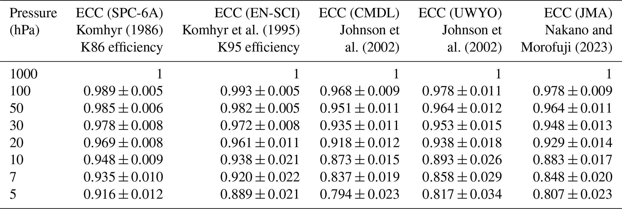
The pump efficiency tables reported by Johnson et al. (2002) and more recently by Nakano and Morofuji (2023) are both based on a large number of pump calibrations using complementary and well-established methods and can therefore be classified as true pump efficiencies. Both tables are generally consistent within statistical uncertainty but diverge significantly from the older Komhyr (1986) and Komhyr et al. (1995) tables. Although the Komhyr tables (K86 and K95) have historically been called “pump efficiencies”, the Komhyr values in Table 1 are now recognized as empirical efficiencies, which combine decreasing pump efficiency, increasing conversion efficiency, and typical memory effects in the background current for the standard buffered solutions SST1.0 and SST0.5 (Tarasick et al., 2021). For consistency with long-term data records, the values reported by Komhyr (1986) and Komhyr et al. (1995) are recommended by ASOPOS 2.0 (Smit et al., 2021) for SPC-6A and SST1.0 and EN-SCI and SST0.5 but are now referred to as the empirical effective K86 efficiency and K95 efficiency, respectively.
Normally, in the pH=7 buffered KI sensing cathode solution, the stoichiometry of the conversion reaction, Reaction (R1), of ozone into iodine is assumed to be 1.00 with an uncertainty of about ±0.03 (Dietz et al., 1973), while the initial absorption efficiency of gaseous ozone into the sensing solution will be 1.00 with an uncertainty of 0.01. These values for ηA and ηC are used in the conventional method of ozonesonde data processing as recommended by ASOPOS in Smit et al. (2021) and before in Smit and the ASOPOS Panel (2014).
2.3 Perspectives on the background current
2.3.1 IB0 and IB1 conventions for background currents
The ECC sensor background current, IB, is defined as the residual current output by the cell when sampling ozone-free air. Since the 1990s, during the preparation of the ECC sensor on the day of flight, two background currents, IB0 and IB1, respectively, have been measured: before and after exposure of a certain amount of ozone, usually about 5 µA ozone equivalent for about 10 min. Both background currents are measured after flushing the cell for 10 min with ozone-free air (Smit and the ASOPOS Panel, 2014; Smit et al., 2021). Although small (typically <0.1 µA), the ECC sensor background current may be of appreciable magnitude compared to the ozone current when there is very low ozone such as in the tropical upper troposphere or in the stratosphere above 5 hPa and also during ozone hole conditions in polar regions.
Background measurements of SPC-5A (older SPC model type, replaced in 1996 by SPC-6A) sondes operated with SST1.0 using ozone-free air showed, before about 1993, typical values of IB0=0.06 ± 0.02 µA and IB1=0.09 ± 0.02 µA, respectively (Smit, 2004). After 1993, for both SPC-5A and SPC-6A, IB0 dropped to values of 0.00–0.03 µA and at the same time IB1 dropped by about 0.06 µA. This may mean that the manufacturer made changes, most likely cleaning or conditioning the electrodes or ion bridge (e.g. less leakage of I2 into the cathode solution). In the past 30 years, both SPC-6A and EN-SCI sondes have shown similarly low IB0 and IB1 values when a high-quality gas filter flushes the cells with ozone-free “zero” air. However, the IB1−IB0 difference of ∼0.03–0.04 µA has stayed the same over decades. This is actually the “chemical” contribution of the overall O3+KI chemistry in the cathode cell to the measured background current after zero-air flushing, whereas IB0 is independent of ozone exposure and assumed to be an inherent property of the ECC sensor. The latter has been demonstrated in several laboratory experiments (Smit et al., 2007; Vömel and Diaz, 2010) and in this study (Sect. 2.3.3).
Theoretically, an ECC sensor in electrochemical equilibrium will produce no current; any current in the absence of ozone or other oxidants must be due to an imbalance of tri-iodide between the anode and cathode cells (Komhyr, 1969). Possible causes of such an imbalance include (i) a leaky ion bridge, (ii) limited mass transfer of residual tri-iodide () in the cathode solution (Thornton and Niazy, 1982), (iii) limited electron transfer at the cathode surface, (iv) an imbalance resulting from cell conditioning or contamination, or (v) previous exposure to ozone. The first three cases represent a background current that may be expected to remain roughly constant and should therefore be subtracted as a best approximation; however, the last two cases, (iv) and (v), should decline according to the response time of the cell (Tarasick et al., 2021).
2.3.2 Constant background current?
In the early days of the ECC, there was no clear distinction between IB0 and IB1 to apply for IB in Eq. (1). Komhyr (1969) suggested that IB resulted largely from a residual sensitivity of the ECC sensor to oxygen and that IB decreased with air pressure in proportion to the rate at which oxygen entered the sensor. Thornton and Niazy (1982) showed in a laboratory study that the primary source of the background current is from the removal of residual tri-iodide, normally present in the cathode solution, and not from the reaction of oxygen with iodide to produce tri-iodide or from the direct reduction in oxygen. Since 1975, the manufacturer (Science Pump Corporation) has preconditioned the ECC electrodes with iodide such that the oxygen dependence has become vanishingly small and can be neglected (Thornton and Niazy, 1982).
2.3.3 Past ozone-dependent background current
Based on simulation chamber experiments, Smit et al. (1994) recommended using IB0 for the constant IB subtraction, which was confirmed in a field experiment by Reid et al. (1996). However, the results could not be confirmed in later JOSIE campaigns, which demonstrated that the background current most likely varies with the past ozone measured, implying that two background currents operate over the sonde operation (Smit and Sträter, 2004a, b; Smit et al., 2007): (i) one background current IB0, which is independent of ozone exposure, and (ii) a second past ozone-dependent background current that will vary in the course of the sounding. This time-variant ECC background current is assumed to result from a minor, but still slowly decaying, contribution to the measured cell current. Based on laboratory experiments, Johnson et al. (2002) and Vömel and Diaz (2010) suggested that its origin is related to the ECC chemistry having a fast pathway (20–30 s) and an additional minor pathway (reaction time constant ∼20–30 min) that causes a memory effect, probably due to slow side reactions in the oxidation of iodide by O3 in the cathode sensing solution. In equilibrium this can lead to an overall stoichiometry factor, , of larger than 1.0 as observed by Johnson et al. (2002). The magnitude of the excess stoichiometry depends strongly on the phosphate buffer concentration in the cathode sensing solution. Vömel and Diaz (2010) suggested that, instead of a measured background current, it would be better to use an appropriate solution-dependent conversion efficiency and background current values in the basic ECC formula, Eq. (1). For improved data processing, the contributions of the slow (20–30 min) and fast (20–30 s) responses to the overall measured ECC ozone signal need to be considered simultaneously using an appropriate response (memory) function.
Such a possible methodology may be the deconvolution of the measured ozone profile after determining the overall frequency response of the combined sensor and air sampling system (De Muer and Malcorps, 1984). However, the method is complicated and not practical to apply to the global ozonesonde network. More accessible are first-order numerical schemes that deconvolve the fast response which were developed and tested by Imai et al. (2013) and Huang et al. (2015). Tarasick et al. (2021) further developed one simple first-order numerical scheme to resolve both the fast and the slow time responses of the ECC sensor. Vömel et al. (2020) developed the methodology for quantifying the fast and slow currents in more detail, but several aspects were not fully considered, and their methodology was not assessed with the most comprehensive database and for various pairs of sonde types and SSTs. This study remedies these gaps.
To investigate the chemical origins of the slow current, laboratory response time tests for hundreds of ECC ozone sensors (EN-SCI, SST0.5) have been made at the Uccle (Belgium) sounding station since August 2017 during every routine day-of-launch preparation to measure the two time constants in the ECC signal. In this experiment, the following steps were taken to record the ECC sensor current as a function of time:
- a.
Before ozone exposure, flush the ECC for 10 min with zero air; record IB0.
- b.
Expose the ECC for 10 min to 5 µA ozone equivalent.
- c.
Flush the ECC for 10 min with zero air; record IB1 and stop flushing (pump inactive, short-circuit sensor leads)
- d.
Do not flush until t=55 min, and then flush 5 min zero air; record IB60, and then stop flushing.
- e.
Do not flush until t=115 min, and then flush 5 min with zero air; record IB120.
The steps (a) to (c) follow exactly Smit and the ASOPOS Panel (2014) and Smit et al. (2021) SOPs. However, after these steps, most of the time between t=10 and t=120 min, flushing with ozone-free air has stopped except for the 5 min periods at t=55 and 115 min. During the 5 min of flushing, a short current increase was observed, but it declined rapidly with a typical “fast” response time of 25 s. The 120 min timing was chosen because this is the typical duration of the ascent of an ozone sounding. Summaries of the observations for the fast and slow currents appear in Fig. 1.
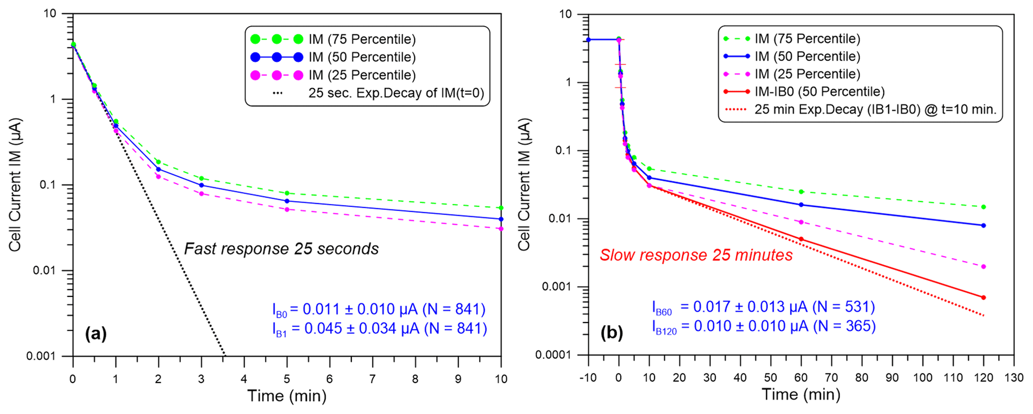
Figure 1Relaxation of the measured ECC current IM(t) (logarithmic scale) flushed with purified ozone-free air as a function of time after the cells have been exposed for 10 min with 5 µA ozone. The sequence is as follows: (i) no flushing t=10 to 55 min, (ii) flushing t=55 to 60 min, (iii) no flushing t=60 to 115 min and (iv) flushing t=115 to 120 min. Displayed are the medians of IM(t) (solid blue line) and its 25th and 75th percentiles (pink and green dashed lines, respectively). (a) The first 10 min relaxation of IM(t): dotted black line, decay of IM (t=0 min) with 25 s time constant. (b) Full 2 h of relaxation of IM(t), solid red line, median of IM(t)−IB0; dotted red line, decay of IB1−IB0 (t=10 min) with 25 min time constant.
The observed relaxations in Fig. 1 follow a typical superposition of two first-order exponential decays of the fast and the slow component, which can be expressed here as
where IF0 and IS0 are the fast-sensor-current and slow-sensor-current contributions, respectively, at the start of the response test at t=0.
Although after t=10 until t=120 min for only two short periods of 5 min the cathode cell was flushed with ozone-free air, the results are consistent with the observations of Vömel and Diaz (2010), who flushed the cathode cell over the entire 120 min relaxation period. Clearly the relaxation of the slow component of the background is independent of the flushing, i.e. no stirring action in the cathode sensing solution, and therefore most likely has a chemical origin from a slow reaction pathway. The IB0 and IB1 shown in Fig. 1 are typical of present-day ECC sondes (e.g. Smit et al., 2021). Further, the characteristic difference in IB1 and IB0 of about 0.03–0.04 µA has been observed over a large number of sondes (≅800) and is most likely the residual of the slow reaction pathway.
In contrast to Vömel and Diaz (2010), based on around 25 runs, in the more than 350 Uccle experiments the cell current does stabilize after a 1–2 h decay time to the background current before exposure to ozone, IB0. As a matter of fact, assuming a 25 min decay from the mean IB1=0.045 µA at t=10 min, the IB60 and IB120 would decay on average down to 0.006 and 0.00055 µA after 60 and 120 min, respectively. Actually, we recorded mean values of 0.017 and 0.010 µA, respectively. The average differences in IB60−IB0 and IB120−IB0 are 0.008 and <0.001 µA, respectively. This indicates that after correcting the measured cell current IM(t) for the constant background current IB0, the residual current IM(t)−IB0 (Fig. 1, solid red line) fits very well with the 25 min decay of the mean IB1−IB0 starting at t=10 min (Fig. 1, dotted red line). Similar observations were made in 1993 in the simulation chamber at WCCOS, whereby four ECC sondes were flushed for more than 90 min with zero-ozone air during the simulation of a tropical descending pressure profile. After a relaxation time of about 70 min, the cell currents approximate constant values, which are very close to the corresponding recorded IB0 (for details see Fig. S1 in the Supplement). This means that after 1–2 h of flushing the ECC sensor with zero ozone, the remaining current is identical to IB0, so during the typical duration of the ascent of an ozone sounding, the remaining current (IB0) persists, which is not the result of a 25 min decay but has another origin. This inherent IB0 of the ECC sensor, possibly caused by a small leakage of iodine (I2) from the ion bridge into the cathode solution or by a mass-transfer limit in the solution or electron transfer at the cathode surface (Thornton and Niazy, 1982, 1983), appears to be constant over the 2 h of an ozone sounding.
To understand the KI+O3 chemistry and the impact of the phosphate buffer on the stoichiometry of the conversion of the sampled ozone into free iodine, Tarasick et al. (2019, 2021) reviewed many studies in which a variety of KI-solution strengths with different pH buffers were investigated. The reaction mechanism of KI+O3 in aqueous solution in the presence of a phosphate buffer as investigated by Saltzman and Gilbert (1959) may explain the observations made here and is discussed in detail in Appendix A. In short, they proposed two reaction pathways: a primary reaction pathway without a buffer and a secondary pathway with a buffer. Experimentally, Saltzman and Gilbert (1959) showed that the impact of the slow reactions increases with the buffer concentration, whereas buffered solutions with no KI showed no evidence of any O3 reactions. This means that the additional reactions with O3 are secondary reactions after the initial O3+KI reaction. Saltzman and Gilbert further demonstrated that the secondary pathway could form additional free iodine, half of it reacting very fast (≪ than 1 s, i.e. the residence time of air sample in the cathode cell) and the other half reacting more slowly (∼25 min). This means that the secondary reaction pathway can contribute to both the fast and the slow ECC current. However, loss mechanisms may occur too. In summary, we do not know exactly the stoichiometry of the fast and slow reaction pathways leading to free iodine. Therefore, we can only indirectly quantify these two stoichiometries that lead to the fast-cell-current and slow-cell-current components observed, respectively. In other words, the measured cell current IM(t) is the superposition of
where IP,F is the sensor current contribution from the fast primary reaction pathway. IS,F is the sensor current contribution from the fast secondary reaction pathway. IS is the sensor current contribution from the slow secondary reaction pathway with a typical 20–25 min time response.
The contribution of the fast reaction pathways that form iodine fast is lumped together in the total fast-sensor-current component IF(t) with a typical time response of 20–30 s. The measured sensor current IM(t) is then expressed as
The overall stoichiometry ST of the chemical conversion of O3 into I2 is the sum of the stoichiometry factors SF and SS of the fast and slow reaction pathways, respectively.
2.4 Formulating new fast and slow components of the ECC current
From the response tests (fast decay from 5 µA down to 0.1–0.5 µA within less than 1 min) it can be concluded that SF is close to 1 (0.9–1.1) and at least a factor 10–20 larger than SS, which is small (0.01–0.10). The timescale of the slow-current component (τS=25 min) is slower by about a factor of 60 compared to the dominating fast-current component. This means that the slow current acts as a slowly time-varying background current. The latter can be treated as a superposition with the ozone-independent background IB0 to constitute the total background but given now as the time-varying IB(t) in Eq. (1).
By substituting IM(t)−IB(t) into Eq. (1), the partial pressure of ozone is now expressed as Eq. (6):
where the fast sensor current is expressed as
The conversion efficiency may depend on the sonde type and sensing solution type. It is largely related to the stoichiometry of the conversion of O3 into I2 from the primary fast reaction pathway and to a lesser degree from the secondary reaction pathway. The partial ozone pressure can be determined from Eqs. (6) and (7) in two steps:
- a.
Determine the slow current as a function of time. Because the past-ozone-exposure-dependent slow-current component IS(t) is much slower and smaller than the fast-current component IF(t), the slow current can be determined from the convolution of the measured current IM(t) with the slow time constant τS=25 min.
- b.
Calculate the fast current IF(t), and then, through deconvolution of IF(t), resolve the time delay of the relatively fast time constant τF=20 to 30 s.
The fast as well as the slow reaction path is determined by a first-order time response and can therefore be separated into a convolution part to determine IS(t) and a deconvolution part to obtain the fast-current component, IF,D(t). The mathematical techniques used here to resolve the impacts of the slow and fast time constants, τS and τF, respectively, are based on the numerical scheme described by Miloshevich et al. (2004) and were first applied by Imai et al. (2013) to resolve the time delay effects caused by the ECC fast response time. A first-order response of a measured sensor signal U (here ECC ozone sensor current) that is approximately proportional to a change in time of U is described by the common “growth law equation”:
where Um is the instantaneous measured signal, Ua is the ambient (“true”) signal that is driving the change in Um and τ is the time constant of the signal.
Integrating Eq. (8) over a small time step gives the measured signal as a function of time:
In cases where the time step Δtk is chosen to be small relative to the response time τ, it can be assumed that the true (ambient) signal Ua is quasi-stationary during time step Δtk such that . The exponential term is the response function.
Equation (9) can be expressed in a numerical convolution or deconvolution scheme. From Eq. (9) we can obtain IS(t) and IF,D(t) as follows in the next two subsections.
Case 1: slow-current component derived from convolution (time constant τS) of the ambient sensor current Ia
To obtain the slow-current component (IS), Um in Eq. (9) is substituted by the slow fraction of Ia, represented here by the stoichiometry SS multiplied with the ambient (true) ozone sensor current Ia. Equation (9) can now be re-written into the integrating form:
whereby the slow-response function XS is
Case 2: deconvolution (time constant τF) of the fast signal IF with τF
To obtain the deconvolved fast-current component IF,D, Eq. (9) should be solved to obtain Ua (=IF,D), and Um is substituted by the fast fraction IF. Equation (9) can then be re-written into the differentiating form:
where the fast-response function XF is
Compared to Vömel et al. (2020), the recursive numerical convolution scheme proposed here (Eq. 10) is the same, while the deconvolution scheme (Eq. 12) differs through the inclusion of the exponential fast-response function XF (Eq. 13) itself, rather than its first-order approximation. The latter allows larger time steps Δtk, which may become significant for older ozone-sounding records that have data with a resolution of 10 s or more.
To resolve the slow and fast time responses of the measured ECC sensor current, the JOSIE measurements conducted in several campaigns between 1996 and 2017 form an ideal dataset for several reasons. Firstly, all the ozonesonde preparations and the measurements were carried out in a controlled environment. Secondly, the availability of simultaneous reference measurements from a fast-response photometer, the OPM, with high precision and accuracy provides an absolute reference for the derived ozone profiles. Further, in the course of the simulation several response tests are performed in which the ozonesondes and the OPM are exposed to zero-ozone air for a 5 min period (see Fig. 2). These response tests enable us to determine the stoichiometry of the slow reaction pathway and subsequently the slow sensor current IS(t) as a function of time. In this sense, the JOSIE 2009/2010 campaign dataset is of particular interest because all experiments included four of those response tests in the simulation profiles themselves.
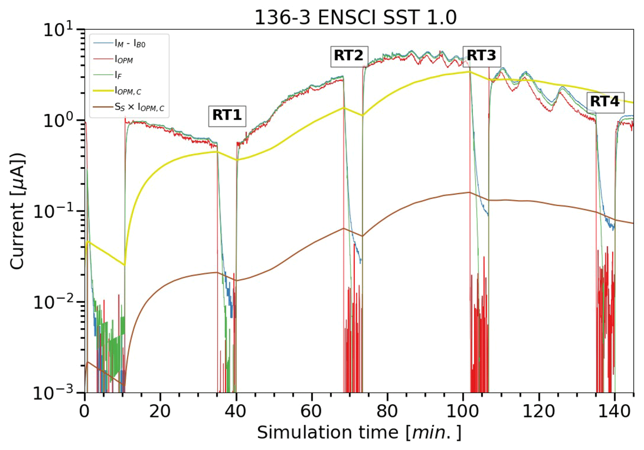
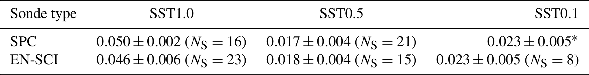
Figure 2Example of a simulation run during JOSIE 2009 as a function of the simulation time, with the measured ECC current IM minus IB0 (blue line); the generic OPM current IOPM (red line); the 25 min convolved IOPM,C (yellow line) and the 25 min convolved IOPM adapted to IM−IB0 after the determination of the slow stoichiometry factor SS or slow current IS (SS×IOPM,C) (brown line); and the fast sensor current IF (green line), obtained after correction of the measured sensor current IM for the constant background current IB0 and the slow-current contribution IS.
For the sake of clarity, it is to be noted that the ozone readings reported here of the OPM are already based on the new UV-absorption cross-section, referred to as the CCQM.O3.2019 (BIPM, 2022; Hodges et al., 2019) value, which is about 1.23 % lower than the former cross-section (Hearn, 1961) that was mostly used before in the global ozone ground-based monitoring networks. In 2024–2025 the new cross-section will be introduced into the global ozone observation networks using UV photometry (BIPM, 2022). Consequently, all measurements of the OPM reported here are about 1.23 % larger than the values reported before in earlier JOSIE publications.
3.1 JOSIE 2009/2010
The JOSIE 2009/2010 protocols are similar to the JOSIE 1998 campaign (Smit and Sträter, 2004a; Smit et al., 2007). In 2009 a set of 40 brand-new ECC sondes (20 SPC6A and 20 EN-SCI) were tested; in 2010 the same set of ECC sondes, refurbished and tested under the same conditions, was evaluated against the same OPM reference. One aim of these campaigns was to test the performance of brand-new and refurbished ozonesondes. It was found that the re-used sondes agree within 1 %–2 % with brand-new sondes, although with a slightly lower precision of ∼5 % (see Fig. 3.1 in Smit et al., 2021). The JOSIE 2009/2010 ozonesondes were prepared by only three operators, strictly following the same preparation protocols, including the use of purified air from the same cylinders for the ozone-free air source. It can therefore be considered an ideal dataset for well-prepared ozonesondes. All ozonesonde data were processed according to the guidelines of Smit et al. (2021), which we denote the “conventional” method hereafter. That means (i) subtracting the constant background current IB1; (ii) correcting the pump flow rate for the moistening effect; (iii) using the empirical effective efficiency tables by Komhyr (1986) and Komhyr et al. (1995) for SPC and EN-SCI ozonesondes, respectively; (iv) converting the measured pump temperature to the internal pump body temperature, with an additional small pressure-dependent correction (Smit et al., 2021); and (v) no total ozone normalization. Note also that all simulations were identical in representing a typical mid-latitude ozone profile (Smit et al., 2007).
During both campaigns, a total of 26 simulation runs were made, of which all but 1 had 4 ozonesondes simultaneously in the simulation chamber, giving a total number of 103 ozonesonde profiles. However, 17 of those profiles were gathered using research-mode SSTs and are not included here. A total of 14 simulations were carried out in December 2009, 2 in January 2010 and 10 in August 2010.
3.2 Determination of slow current IS(t)
3.2.1 Determination of stoichiometry SS
To determine the relative contribution SS of the slow component in the ECC ozonesonde signal, in other words, the stoichiometry factor of the slow reaction pathway of the conversion of O3 into I2, the response tests of the JOSIE 2009/2010 dataset are used. Four time response tests are included during these simulations at four different pressure levels (RT1: 475–375 hPa, RT2: 100–85 hPa, RT3: 20–15 hPa, RT4: 6–5 hPa), during which ozone-free air is provided in the simulation chamber for 5 min. A typical example of a JOSIE 2009 simulation run is given in Fig. 2. After 5 min the fast sensor current has declined by more than sixteen relaxation times and is negligible. This means that at the end of this time response test, the only contribution to the overall measured current IM(t), after correction for IB0, comes from the remaining slow-current component. At this moment, the fast co-existing OPM data (red in Fig. 2) provide the true value of the ozonesonde signal. The next paragraphs outline the different practical steps.
To obtain a direct measure of the true ECC ozone sensor current, the OPM ozone partial pressure is converted to the generic OPM current (IOPM) for each individual ozonesonde using sonde pump temperature, the sonde pump flow rate and true pump efficiency values of JMA (Nakano and Morofuji, 2023; see Table 1), as in Eq. (1).
In other words, we are calculating the generic sensor current corresponding to the ozone equivalent measured by the OPM as if it were the true ECC ozone current. This means that the generic IOPM is taken as the actual reference (true) current for determining the slow stoichiometry factor SS.
Additionally, the generic OPM current IOPM (red in Fig. 2) is convolved into IOPM,C with an exponential time response with τs=25 min using Eq. (9) to obtain a slow time response in the generic OPM current signal (yellow in Fig. 2).
Finally, the slow stoichiometry factor SS is obtained by taking the ratio of the remaining ECC sensor current IM minus the constant background current IB0 and the convolved OPM signal (IOPM,C), at the end of the time response test intervals RT1, RT2, RT3 and RT4, when only the slow component is expected to contribute to the sonde signal, such that
The ratios used to obtain the slow stoichiometry factor (SS) values are calculated during the final 50 s of each time response test, RT1, RT2, RT3 and RT4, respectively. Those values, obtained for all ozone profiles within each sonde type and SST combination, are shown in Fig. 3, together with the median and 25th and 75th percentile values. The median SS values and their median absolute deviation (MAD) uncertainties are given in Table 2. Note that the determination of the median SS values (and their uncertainties) is very robust and does not depend on the time response test interval or the slow time lag constant. We will come back to this in Sect. 6.2. Further it shows that by varying τS=25 min by ±5 min, the corresponding SS values only changed by less than 5 %, which is small compared to the MAD uncertainty in Ss (Table 2).
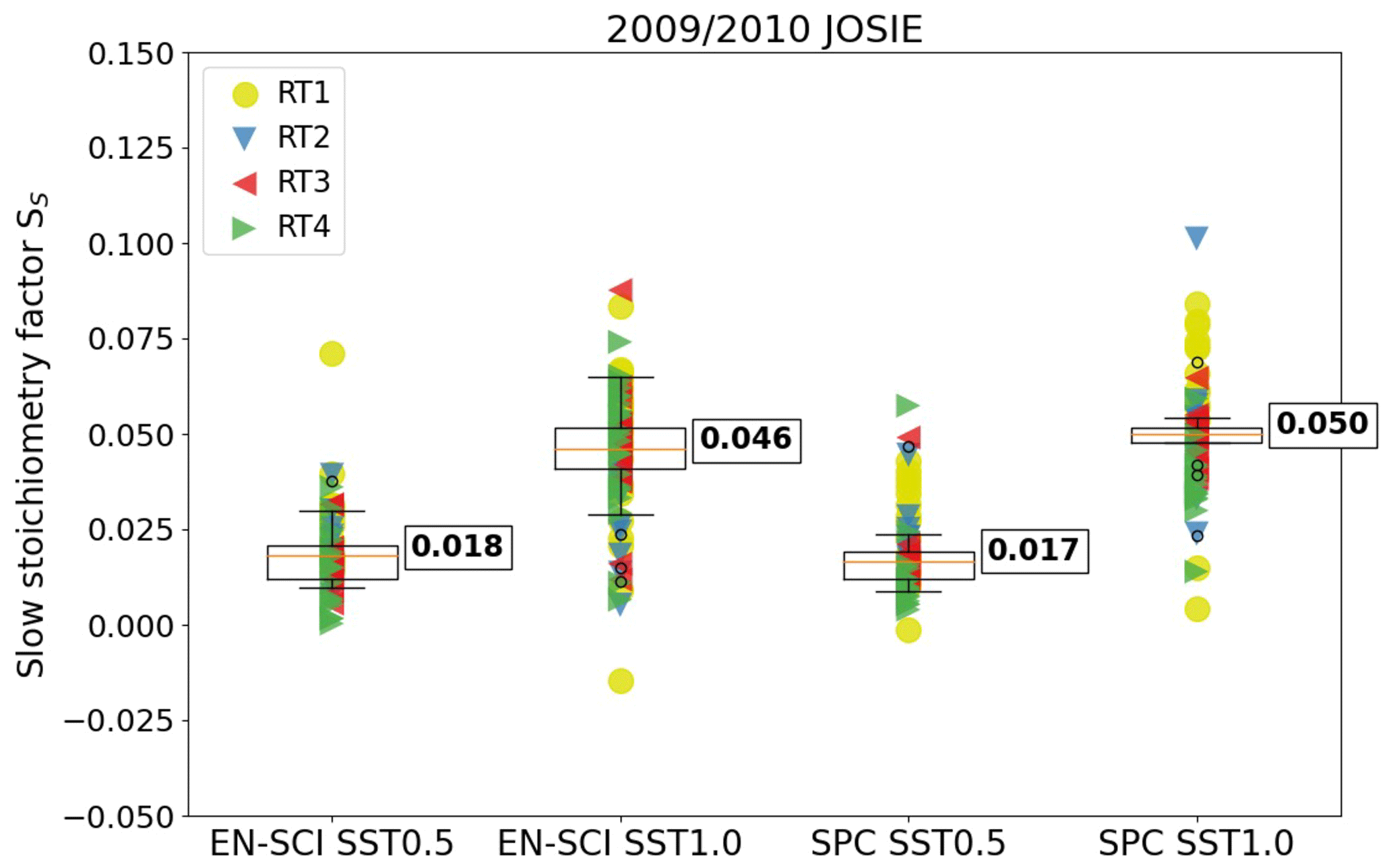
Figure 3Box–whisker plots of the slow stoichiometry factor SS as the ratio of the measured IM minus IB0 to the 25 min convolved OPM current (IOPM,C) obtained from JOSIE 2009/2010 for EN-SCI and SPC ozonesondes operated with SST0.5 and SST1.0. The yellow dots and triangle symbols (blue, red and green) represent the individual values obtained from the four response tests RT1, RT2, RT3 and RT4, respectively. Thus, every ozonesonde profile is represented four times in the graph. The Box–whisker plots are represented by the median plus the 25th and 75th percentiles (horizontal orange and black lines, respectively, for each pair of instrument–SST combination).
Table 2Median and its median absolute deviation (MAD) uncertainty values of the slow stoichiometry factor SS obtained from JOSIE 2009/2010 for SPC and EN-SCI ozonesondes operated with the sensing solution types SST0.5 and SST1.0. The stoichiometry factor SS for EN-SCI–SST0.1 has been determined with the same approach but using laboratory measurements at Uccle with an ozone reference instrument (see Appendix B).
∗ The same value for SPC–SST0.1 has been adopted as for EN-SCI 1.0 %-0.1B. NS is the number of sonde profiles.
The most striking feature is that SS only depends on the SST and not on the sonde type. This confirms our hypothesis on the origin of this slow component, as described in Sect. 2.4. For SST0.5 and SST1.0 there is an almost proportional relation between the magnitude of SS and the buffer strength. Johnson et al. (2002) have demonstrated that an increase in the stoichiometry is primarily caused by the buffer strength with only a minor contribution of the KI concentration. This result might be explained by the secondary reaction pathway of the reaction mechanism after Saltzman and Gilbert (1959), whereby the extra slow stoichiometry contribution is caused by the buffer (Appendix A). However, a comparable result does not hold for SST0.1 (Table 2). One would expect that for the low buffered case (SST0.1) SS should be much smaller than for SST0.5. This is not true; SS is even slightly larger. It seems that for SST0.1, other competing reaction mechanisms may occur, which do depend on the KI concentration, and may generate free iodine on a 25 min timescale. Such a hypothetical mechanism may also explain the fact that for low or not buffered SST we still measure IB1 background currents with values of 0.01–0.03 µA larger than IB0 as measured in JOSIE 2000 (no-buffer SST; Smit and Sträter, 2004b) and JOSIE 2017 (SST0.1; Thompson et al., 2019). A speculative mechanism is that the electronically excited oxygen singlet molecule formed in Reaction (AR3) of the primary reaction pathway of the O3+KI chemistry (Appendix A) may either be deactivated in Reaction (AR5) or react with H2O and produce hydrogen peroxide (H2O2) (e.g. Xu et al., 2002). The H2O2 formed would oxidize KI to produce free iodine but on a timescale of 25 min, which could contribute to the slow current IS(t). Further studies are required to understand the underlying chemical processes.
The stoichiometry factors SS (Table 2) to determine the slow current IS(t) are substantially lower than the so-called “steady-state bias factors” applied by Vömel et al. (2020). These steady-state bias factors were determined as the overall excess fraction of the stoichiometry of 1.00 from laboratory experiments with a fixed ozone exposure over several hours (Figs. 3 and 4 in Vömel and Diaz, 2010). In this study we derived for SST1.0 SS=0.046 to 0.050 which is only half the 0.09 value of Vömel et al. (2020). For SST0.5 and SST0.1, our respective SS=0.017 to 0.018 and 0.023 values are also smaller than their 0.024 and 0.031 steady-state bias factors. Using the same laboratory procedures as Vömel and Diaz (2010), Johnson et al. (2002) reported an excess overall stoichiometry of ∼0.07 for SST1.0. The lower factors obtained in this study, particularly for SST1.0, might also be related to the different methodology followed for determining SS. Here, SS values are determined from the response of a downward step under zero-ozone conditions. In Johnson et al. (2002) and Vömel and Diaz (2010) the excess stoichiometry factors were determined from the relatively small differences observed between the ECC sonde and a reference UV photometer after a 60 min upward-step ozone exposure. The latter requires very accurate generation of ozone values with a precision better than 1 % to determine the relatively small excess stoichiometry factors involved. Also note that for the earlier studies, reference ozone readings are based on an older UV-absorption cross-section (Hearn, 1961) that are now corrected by 1.23 % to be compatible with the new UV-absorption cross-section (Hodges et al., 2019) applied to the OPM. Accordingly, the steady-state bias factors of Johnson et al. (2002) and Vömel et al. (2020) should be decreased by subtracting 0.012. The resulting SS values would then approach the SS values obtained here for SST0.1 and SST0.5 and better approximate the SST1.0 SS values.
Another difference between the new methodology and that of Vömel and Diaz (2010) is that we subtract IB0 from the ozonesonde signal prior to determining the stoichiometry. However, we also determined the SS values without correction of IB0; the results appear in Fig. S2. It is noted that these SS values increase for all sensing solution types by only 0.005–0.009. For SST0.5 and SST0.1, they approach the Vömel and Diaz (2010) values, but the substantially lower SS values for SST1.0, as derived here (Table 2), cannot be explained exclusively by subtracting IB0. Furthermore, comparing Fig. 3 with Fig. S2 also demonstrates that the subtraction of the IB0 value makes the determination of the SS values even more independent of the selected RT intervals, which is not the case without this prior subtraction (e.g. the RT1 values being significantly larger than the other RT values).
The factors reported by Johnson et al. (2002) and Vömel and Diaz (2010) are based on a limited sample of experiments (three different sondes using three different solutions for a total of 22 runs in Vömel and Diaz, 2010) in contrast to the large statistical sample in this study (Table 2). The difference between the two approaches – in terms of exposure to ozone or not – may be then explained by assuming that when the overall excess stoichiometry originates from the secondary reaction pathway, only half of it contributes to the slow cell current IS(t) with the other half contributing to the fast cell current IF(t). For SST0.5 and this SST1.0, this can be understood by the types of reaction mechanisms of the secondary reaction pathway as proposed by Saltzman and Gilbert (1959): in this case, about half of the extra stoichiometry caused by the buffer could be still contributing to the relatively fast signal (Reaction AR7) and the other half to the slow signal (Reaction AR8) (see Appendix A). This would mean that the stoichiometry of the secondary reaction pathway could be 2 times the stoichiometry factor SS of the slow ECC current IS(t) determined here from the response tests RT1 to RT4 after IF(t)=0. However, for the SS values for SST0.1, which are even slightly larger than for SST0.5, explanations would be more speculative. More analysis and new JOSIE trials might be required to find the cause of varying factors among the different studies and SSTs.
3.2.2 Initial condition of slow current IS(t)
With the derived SS values, the slow component of the sonde signal (IS) is computed by convolution with the slow time constant τs=25 min, as in Eq. (10) (brown line in Fig. 2). Note that, in practice, to determine IS(t), the measured current IM(t) minus IB0 can be taken instead of the true generic ozone current IOPM(t) because their differences are rather small (less than 5 %–10 %); at the same time the slow stoichiometry factors SS are also smaller than 0.1. From here on, we will use the measured current IM(t) minus IB0 to determine the slow current IS(t) along with the SS values listed in Table 2.
As Eq. (10) is a recursive expression, the initial conditions of IS reflect prior ozone exposure during pre-launch preparations, although they decay exponentially in time. Exposure to ozone values during pre-launch will cause non-zero IS values at the beginning of the simulation, impacting the boundary layer ozone profile (e.g. Fig. 10 in Vömel et al., 2020). Ideally, the convolution of the slow component of the sonde signal is computed taking the pre-launch measurements into account. These pre-launch measurements are available for JOSIE 2009/2010 (as in Fig. 4), but this is often not the case for operational soundings. Using those JOSIE 2009/2010 pre-launch simulation data (with negative simulation times in Fig. 4), we found that the best approximation of the true IS (dashed red line in Fig. 4, taking all the pre-launch measurements into account) is obtained if IS(t0) equals IB1−IB0 multiplied with the exponential decay factor , where Δt is the time interval between the measurement of IB1 and the start of the launch (dashed green line in Fig. 4). It is important to mention here the good agreement of the measured IB1 value (horizontal yellow line in Fig. 4, subtracted by IB0) with the convolved, pre-launch, slow component IS (dashed red line) at s (time mark no. 2 in Fig. 4). This reinforces the selection of the IB1−IB0 measurement as a good pre-launch representation of the slow component of the ECC signal.
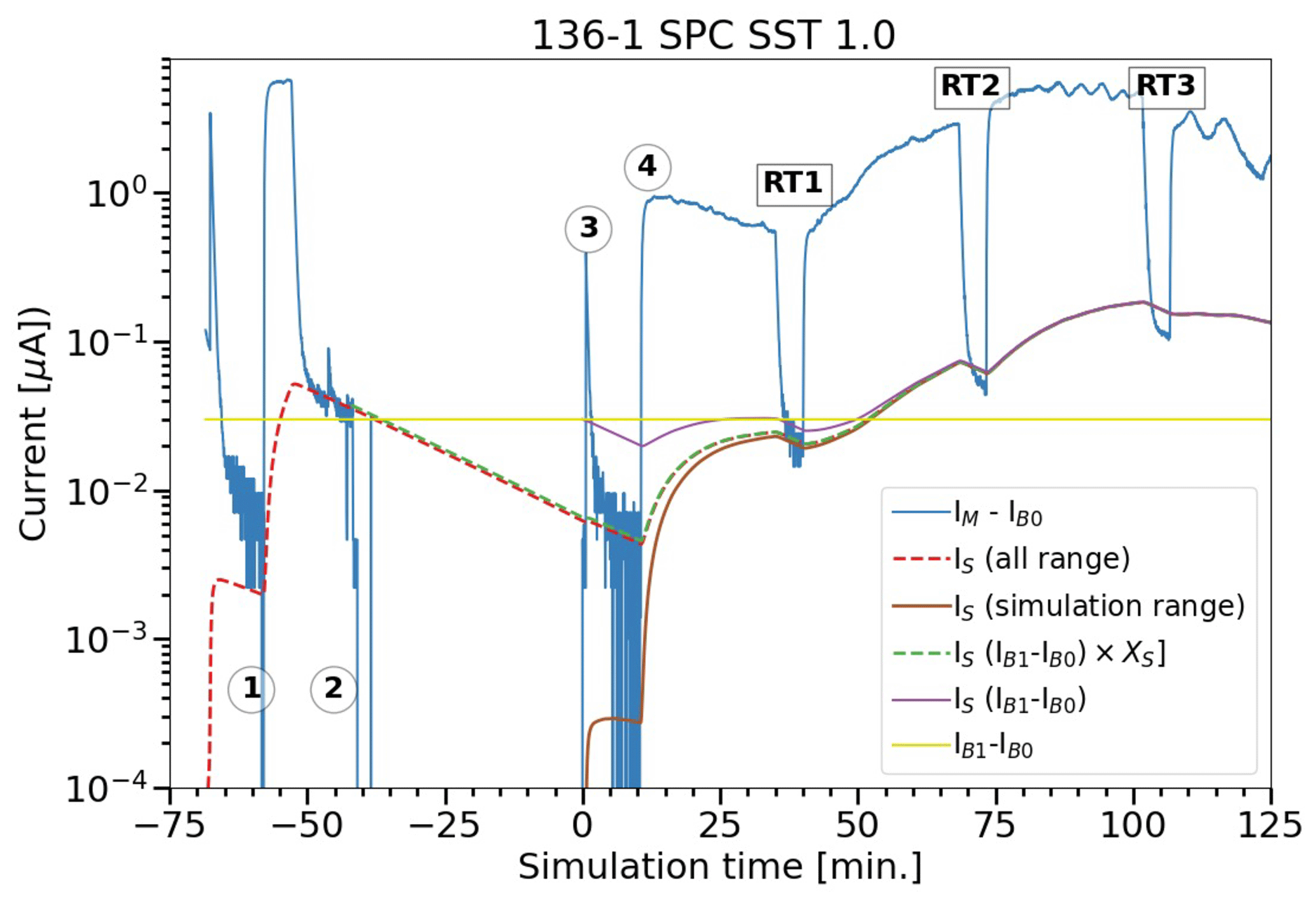
Figure 4Convolved slow ECC current obtained from different initialization scenarios as a function of the simulation time (for details see text). The dashed red line is the convolved ECC current obtained from the measured IM minus IB0, hereby including all pre-launch measurements (with negative simulation times). Time stamps 1–4: 1, record IB0; 2, record IB1; 3, turn on pump motor (at simulation time t=0); and 4, start ozone profile of simulation. RT1, RT2 and RT3 are the first three in-flight time response tests. Slow current IS(t) derived with four different start scenarios: (i) all range (IS=0 at min, dashed red line), (ii) simulation range (IS=0 at t=0 min, solid brown line), (iii) at time stamp 2 with 25 min exponential decay XS (dashed green line) and (iv) at time stamp 3 (solid purple line).
To apply this method in the ozonesonde network, it is essential to record the time difference between the IB1 measurement and the sonde launch. In Smit et al. (2021), the recording of the IB1 time stamp is included in the SOPs for ozonesonde preparations. For the JOSIE 2009/2010 data, we will use this exponential decay method for the initial condition of the convolved slow component at t=0. For the initial condition of the slow component IS(t0), we investigated two other alternatives:
-
, denoted by the horizontal yellow line in Fig. 4, which results in a slow component IS marked by the solid purple line, which clearly overestimates the true IS at the beginning of the profile (up to about 3500 s).
-
IS(t0)=0, for which the corresponding IS, represented by the solid brown line in Fig. 4, underestimates the true IS for up to about a simulation time of 2200 s for the JOSIE 2009/2010 representative example here.
For stations with a time gap of several hours between the IB1 measurement and the launch time, the current will have fallen back to IB0 (see the Uccle example in Fig. 1), resulting, after subtraction of IB0, in this particular case in IS(t0)=0.
A better understanding of the ECC time response provided a justification for quality control indicators for IB0 (<0.03 µA) and IB1 (<0.07 µA) in Smit et al. (2021). In practice, often higher background currents for IB0 and IB1 are recorded at the sounding sites on the day of the launch. These high background currents are typically caused by the use of an inadequate gas filter in the test unit; e.g. the filter provides ozone-free air but does not trap water vapour and contaminants in the laboratory air that is filtered into the preparation equipment. A poor filter combined with a leaky photolysis cuvette producing ozone by UV photodissociation of oxygen with a Hg-discharge lamp can contaminate the airflow to produce high-background-current measurements. It appears that UV irradiation can produce substances that may also react with KI to produce iodine similar to KI and O3. There are some indications (Newton et al., 2016) that high backgrounds may be due to processes with decay times ∼25 min like the slow cell current IS(t). Nevertheless, more research is necessary to investigate the cause and the time behaviour of these high background currents in the course of the sounding in order to correct for this artefact properly. As stated by ASOPOS 2.0 (Smit et al., 2021), the use of proper gas filters to provide ozone-free, dry and purified air in practice at the sounding site is essential not only in general, but also when applying the data processing proposed here.
3.3 Determination of the fast ECC ozone sensor current, IF(t)
After determining the slow component of the signal due to the secondary reaction pathway, we can subtract it from the overall measured current IM−IB0 to end up with the fast component IF (Eq. 7), as shown by the green line in Fig. 2. From the fast component IF(t), we can remove the time lag introduced by the time response of about 20–30 s through deconvolution of IF(t) according to Eq. (12). In this paper, we use τF=25 ± 4 s for EN-SCI and τF=21 ± 4 s for SPC ozonesondes, which are the average fast time responses determined from all the simulation time response tests (RT1, RT2, RT3, RT4) during JOSIE 2009/2010. The response times of the EN-SCI sondes are typically about 4 s longer than the SPC-6A sondes due to the slightly lower pump flow rates and slightly larger volume of the cathode cell of the EN-SCI sondes (Smit and Sträter, 2004a). In general, we found that the fast response times in the upward as well as in the downward direction agree within 1–2 s. Moreover, τF only varies marginally in flight with a slight decrease of less than 5 %–10 % between the surface (RT1) and the upper part of the sounding (RT4). The in-flight τF values also agree very well with the τF values determined from the response tests made during the pre-flight preparation of the ECC sensor, which confirmed earlier observations made during JOSIE (Smit and Sträter, 2004a). A close-up of the first time response interval RT1 is provided in Fig. 5, in which the deconvolved fast component is also shown in yellow.
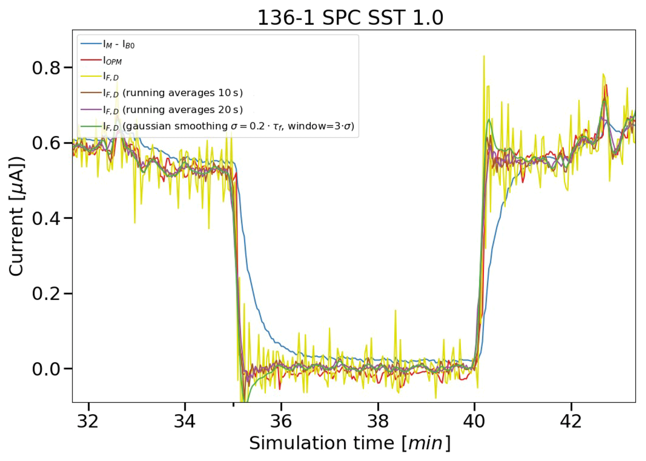
Figure 5Example of a downward and upward response of a simulation run in the tropospheric part of the vertical profile to show the impact of resolving the fast-response effects on the measured cell current IM minus IB0 (IM−IB0: solid blue line). The fast, deconvolved current IF,D without smoothing is shown in yellow and with a moving average smoothing over a time interval of 10 and 20 s in brown and purple, respectively. The Gaussian smoothing applied to IF,D and used in this paper is marked by the green line. For reference, the OPM current is shown in red.
Note that the deconvolution procedure introduces a substantial amount of noise into the data. To reduce this noise, the deconvolved current signal should be smoothed. We therefore used a smoothing with a Gaussian filter with width equal to 20 % of the time lag constant τF as in Vömel et al. (2020), their Eqs. (10) and (11). Compared to other common smoothing techniques, e.g. running averages with a time window of 10 s (see brown line in Fig. 5), this Gaussian filter still has a slight phase shift with respect to the true signal (IOPM, in red in Fig. 5) but outperforms other tested smoothing algorithms in terms of reducing the noise level. The final smoothed, deconvolved signal is shown in green in Fig. 5. It is obvious that, after correcting for the slow and the fast time responses in the signal, the resulting current better agrees with the OPM current than the original measured current. It even exhibits small-scale features that are also present in the fast(er) response OPM measurements. The remaining small differences indicate that the conversion efficiency, i.e. stoichiometry of the fast reaction, slightly deviates from 1.
To test the time response correction (abbreviated here as TRC) methodology as described in the previous section and a first version in Vömel et al. (2020), we apply the methodology to individual ozonesonde profiles of the different JOSIE simulations and compare those corrected profiles with the corresponding OPM measurements. This method involves the use of the stoichiometry factors SS from Table 2 for the different ozonesonde–SST pairs and the application of the measured true pump efficiency factors of Nakano and Morofuji (2023) (Table 1). In contrast to this TRC method, ozone partial pressures from profiles are determined according to the conventional method, as recommended in ASOPOS (Smit and the ASOPOS Panel, 2014; Smit et al., 2021), e.g. using the constant background IB1 correction with the Komhyr (1986) and Komhyr et al. (1995) empirical effective efficiency factors (Table 1). The comparisons are made for two different JOSIE campaigns: (i) JOSIE 2009/2010 with mid-latitude profiles and well-established ozonesonde preparation procedures and (ii) the JOSIE 2017 campaign with mostly tropical profiles and good ozonesonde preparation procedures.
All comparisons of the TRC method with the conventional method are processed as a function of flight time. However, to present the results as vertical profiles, they are mapped on a pressure grid with successive pressure levels of between 1000 and 5–6 hPa. Hereby, all presented JOSIE campaigns are based on a pressure, temperature and ozone profile simulating a balloon ascent velocity of about 5 m s−1 such that a quasi-realistic linking between the simulated flight time and pressure scale is obtained.
4.1 Ozone profiles from JOSIE 2009/2010 for SST1.0 and SST0.5
In Fig. 6, the relative differences with the OPM for the conventionally processed (left part of each panel) and TRC-processed (right part of each panel) ozonesonde profiles of JOSIE 2009/2010 are shown for each pair of sonde (SPC6A or EN-SCI) and solution type (SST0.5 or SST1.0), respectively, including the mean (solid black lines) and its 1σ standard deviation. The absolute ozone partial pressure differences are presented in the Supplement (Fig. S3).
Figure 6JOSIE 2009/2010: relative differences with the OPM for the conventionally processed (left part of each panel) and TRC-processed (right part of each panel) ozonesonde profiles for four pairs of sonde type and SST shown as scatterplots in four different colours in panels (a)–(d): SPC6A–SST1.0 (a, blue dots), EN-SCI–SST0.5 (b, red dots), SPC6A–SST0.5 (c, green dots) and EN-SCI–SST1.0 (d, brown dots). In each diagram for both methods the mean and 1σ standard deviation of the relative differences are included (solid black line). The dashed black lines in the TRC diagrams are the linear regressions of the difference of the ozonesonde from the OPM as a function of the pressure (on a log 10 scale). A summary plot is provided in Fig. S4, and absolute differences are available in Fig. S3.
For the conventional method, large relative deviations from the OPM exist in the pressure intervals response time tests (in particular RT1, RT2, RT3) included in a simulation. This can be explained by the difference in response time between the OPM and the ozonesondes and the fact that when ozone concentrations are close to zero, the relative differences will be magnified. The TRC method is able to correct well for the time response differences, as illustrated by the small relative differences, although with higher uncertainty (1σ standard deviation) compared to adjacent pressure levels. A major improvement of the TRC methodology compared to the conventional corrections is the fact that the relative differences with respect to the OPM are almost pressure-independent and hence past ozone exposures. Up to about 13 hPa (Z≈30 km), only a slightly increasing bias with decreasing pressure exists between the overall mean of the TRC-corrected ozonesondes and OPM for the JOSIE 2009/2010 sample (dashed black linear regression lines in Fig. 6).
At pressures lower than 13 hPa, the SPC sondes exhibit a declining behaviour, which is discussed in the next section. Overall, both EN-SCI–SST0.5 and SPC–SST1.0 agree very well within a few percent, with the TRC methodology using the correct pump efficiencies (see also Fig. S4). Consistent with earlier JOSIE and BESOS campaigns (Smit et al., 2007; Deshler et al., 2008), for both sonde types, SST0.5 gives around 3 %–5 % lower ozonesonde readings than SST1.0, whereas, for both SSTs, SPC ozonesondes read ∼3 %–5 % lower than EN-SCI.
4.2 Ozone profiles from JOSIE 2017 for SST1.0, SST0.5 and SST0.1
During the JOSIE 2017 campaign, tropical ozone profiles were simulated for three different SSTs: SST1.0, SST0.5 and SST0.1 (Thompson et al., 2019). No time-response tests were performed during these simulations. Therefore, for SST1.0 and SST0.5, the stoichiometry factors, SS, derived from the JOSIE 2009/2010 data have been applied. However, the SST0.1 solution was not tested during the JOSIE 2009/2010 campaign. Therefore, for this SST, we determined the stoichiometry factors SS with the same method as described in Sect. 3.2.1 but with time-response tests during ozonesonde laboratory measurements with a calibrated ozone analyser (details in Appendix B). The derived SS factor is 0.023 ± 0.005. For the JOSIE 2017 campaign data, the initial value of the slow-current component IS at the start of the simulation at t=0 (Sect. 3.2.2) has been chosen to equal 0 (i.e. equal to IB0 before subtracting IB0), as there were usually a few hours between the end of the day-of-launch preparations and the start of the simulation such that IB1 has decayed to IB0.
The differences of the JOSIE 2017 ozonesonde profiles from the corresponding OPM profile using the conventional and TRC data-processing methodologies are shown in Fig. 7; the absolute differences appear in Fig. S5. The most prominent feature for the conventional corrections, sonde type–SST combinations, is the dependence of the sonde on OPM differences in pressure or measured ozone amounts: the mean relative differences (as well as the corresponding standard deviations) are largest just below the tropopause at ∼ (100–200) hPa, where the ozone partial pressures are minimal. The mean relative differences increase with decreasing pressure in both the troposphere and the stratosphere (also obvious in Fig. S6) and are most pronounced in the tropics, where the ozone concentrations can be very low near the tropopause. In contrast, when the TRC method is applied to the data, the pressure–ozone amount dependence of the relative difference almost completely disappears. For the standard EN-SCI–SST0.5 and SPC–SST1.0, there remains a slightly increasing bias with decreasing pressure (dashed black lines), while for the SST0.1 ozonesonde simulations, there is a tendency for decreasing (negative) relative differences with decreasing pressure. For both SPC and EN-SCI, SST0.1 ozone readings are slightly lower than the OPM-measured ozone concentrations in the stratosphere and up to 10 % lower than the ozone values measured with the SOP-recommended solutions (SPC–SST1.0 and EN-SCI–SST0.5).
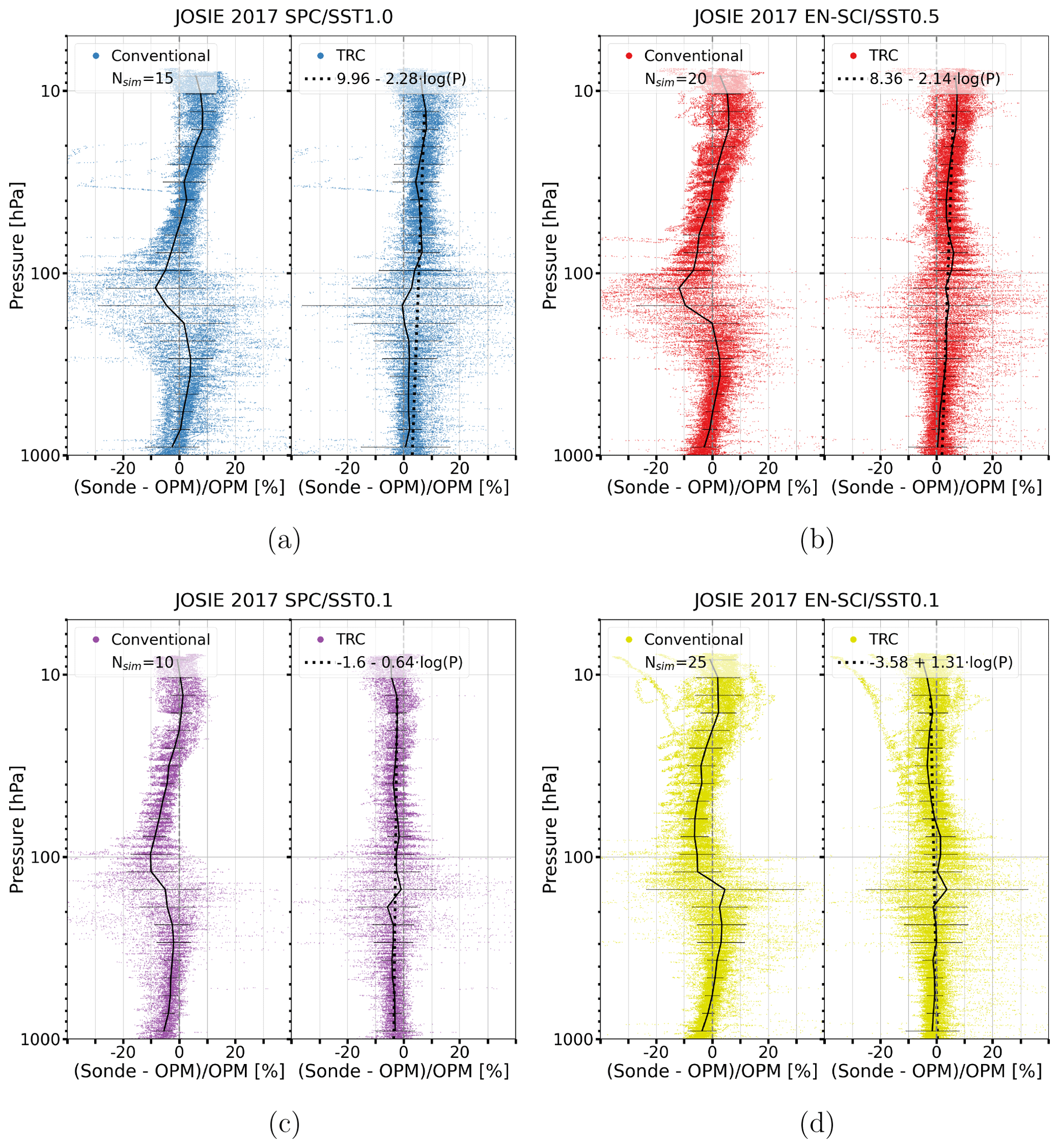
Figure 7JOSIE 2017: differences with the OPM for the conventionally processed (left part of each panel) and TRC-processed (right part of each panel) ozonesonde profiles for the four sonde–SST pairs as scatterplots: SPC6A–SST1.0 (a, blue dots), EN-SCI–SST0.5 (b, red dots), SPC6A–SST0.1 (c, purple dots) and EN-SCI–SST0.1 (d, yellow dots). In each diagram for both methods, mean and 1σ standard deviations are solid black lines. The dashed black lines in the TRC diagrams are the linear regressions of the sonde–OPM differences as a function of the pressure on a log 10 scale. A summary plot appears in Fig. S6, and absolute differences are in Fig. S5.
When comparing the mean relative OPM offsets after processing the ozonesonde measurements with the TRC methodology for the two JOSIE campaigns, e.g. Figs. 6 and 7 (also in Figs. S4 and S6), we note that the network standards SPC–SST1.0 and EN-SCI–SST0.5 are a few percent larger in the stratosphere for the “tropical” JOSIE 2017 campaign. That is, those mean relative differences are manifest in both cases as a slightly decreasing relative bias with increasing pressure during both campaigns. These differences are independent of post-ozone exposure and profile type (mid-latitude or tropical), in contrast to the conventional methodology which exhibits this past ozone memory effect. A striking disagreement between the profile–OPM offsets between JOSIE 2009/2010 and 2017 occurs at the lowest pressure range, lower than ∼13 hPa. For the JOSIE 2009/2010 data, the mean relative differences with the OPM display a stronger pressure dependence in this lowest pressure range, distinctly different for both sonde types, in contrast to the JOSIE 2017 mean relative OPM differences. The origin of this different behaviour above 13 hPa lies most likely in pump temperature differences between the simulated profiles. Whereas the mean pump temperature is close to 21 ∘C in this pressure range in JOSIE 2009/2010, it is around 15 ∘C for the tropical profiles in JOSIE 2017. Simultaneous temperature measurements during JOSIE 2017 revealed that the cell temperatures are about 5 to 10 ∘C lower than the corresponding pump temperatures, depending on the sonde type. Specifically, the differences between pump and cell temperature are more at the high-end range of this temperature interval for EN-SCI sondes, and at the low-end range for the SPC due to differences in thermal contact between cells and pump. With these cell temperatures and taking the boiling temperatures at those low pressures into account, it turns out that the solutions in the SPC sondes tested in JOSIE 2009/2010 may already start boiling at higher ambient air pressures than during JOSIE 2017. Cell weights were measured before and after all simulations for both campaigns. The weight loss due to evaporation or spraying (e.g. when boiling) of the sensing solution was considerably higher during JOSIE 2009/2010 than in JOSIE 2017: about a factor of 2 for EN-SCI–SST0.5 and even a factor of 3 for SPC–SST1.0. Although at these reduced ambient air pressures the absorption efficiency is not critical (Tarasick et al., 2021), the sensing solution losses of the sondes may have become so large during JOSIE 2009/2010 that the absorption efficiency has non-negligibly declined. This may explain the underestimation of the ozone concentrations at low pressures for the JOSIE 2009/2010 profile simulations, in particular for SPC ozonesondes.
5.1 Differences between different pairs of sonde type and SST
In the previous section it was shown that the TRC method resolves the dependence of the measured ozonesonde profile from the past ozone exposure, whereas the deconvolution of the remaining fast ozone sensor current effectively resolves the impact of gradients in the profile caused by the 20–30 s time response of the ECC sensor. The sonde-to-OPM comparisons presented in Sect. 4 for the mid-latitude profiles of JOSIE 2009/2010 (Fig. 6) and tropical profiles of JOSIE 2017 (Fig. 7) demonstrate that the TRC results are independent of the shape of the simulated ozone profiles, in contrast to the results obtained by the conventional method (e.g. Smit et al., 2007; Deshler et al., 2008, 2017; Thompson et al., 2019).
For each pair of ozonesonde type and SST for JOSIE 2009/2010, JOSIE 2017, and combined JOSIE 2009/2010 and 2017 (for SPC–SST1.0 and EN-SCI–SST0.5) a linear regression has been calculated as a function of pressure on a logarithmic scale for the TRC sonde–OPM relative differences within ±30 % for pressures up to 13 hPa. These linear regression lines are shown in Figs. 6 and 7 as dashed black curves in the TRC diagrams for the different sonde–SST pairs; they agree well with the corresponding averages (solid black lines in TRC diagrams). All TRC sonde–SST pair relative-difference scatterplots display variations within 3 %–7 % with altitude between the surface at P=1000 hPa and the upper end of the profile at P=10 hPa, as can be seen in Table 3, which displays the relative sonde–OPM differences at the intercepts P=1000 hPa and P=10 hPa of the linear regression. Table 3 illustrates the same typical differences of 3 %–5 % for the same sonde type but different sensing solutions, SST1.0 or SST0.5, as first observed in JOSIE 2000 (Smit et al., 2007). Figures S4a and b and S6a and b show the persistence of these systematic differences in detail for the conventional and TRC method as a function of pressure (i.e. altitude). The low buffered (SST0.1) EN-SCI or SPC-6A sondes slightly underestimate ozone by a few percent compared to the OPM. It is noteworthy that the EN-SCI–SST0.1 OPM offsets decrease over the course of the sounding, in contrast to all other sonde–SST pairs for which the relative differences increase (Table 3, last column).
Table 3Relative differences of the sonde from the OPM at the P=1000 hPa and P=10 hPa intercepts of the linear regression as a function of log10(P) obtained from the different JOSIE datasets (Figs. 6 and 7) and for the sonde pairs SPC-6A and EN-SCI with different sensing solutions: SST1.0, STT0.5 and SST0.1. Also included are the relative differences between EN-SCI and SPC6A sondes when operated at the same SST (last three rows).
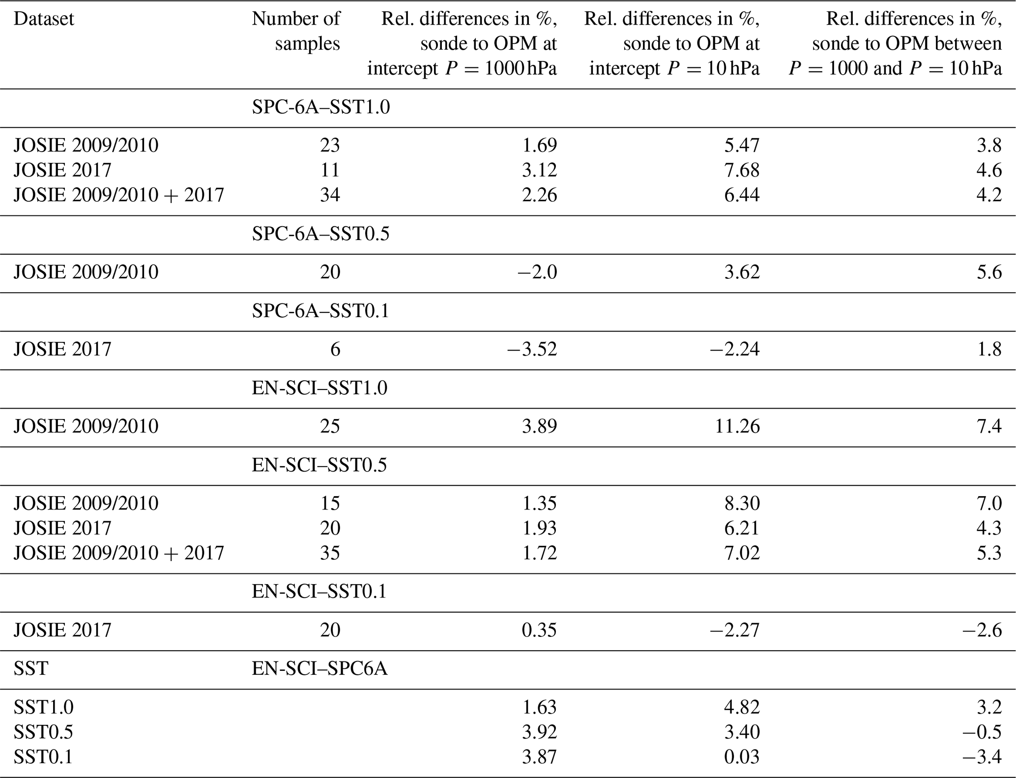
Further, the TRC results show a strong consistency of the mean relative differences with the OPM for the different sonde type–SST combinations across the different (grouped) JOSIE campaigns (see also Figs. S4 and S6). Therefore, those relative mean differences can be characterized by the linear regression curves as a function of log 10(P) in Figs. 6 and 7 and directly linked to the OPM. As such, these linear regression lines (hereafter referred to as “calibration curves”) could be applied as the final correction step of the TRCC methodology (TRC with the application of calibration functions), tracing the ozonesonde measurements back to the OPM as the reference instrument.
5.2 Parameterization of the overall conversion efficiency ηC
The linear regressions of the relative differences of the sonde from the OPM (Figs. 6 and 7) of the TRC method can be interpreted as the correction term of the overall conversion efficiency ηC when deviating from 1 for each of the different pairs of sonde type and SST. The overall conversion efficiency ηC in Eq. (6) can be expressed as a function of the ambient air pressure of the vertical sounding:
where FC(P) is the so-called correctional term of ηC as a function of the ambient air pressure P, which is parameterized by the linear regression fit of the relative sonde–OPM deviations as a function of log10(P) and substituted in Eq. (17). This means that the overall conversion efficiency ηC(P), calibrated to the OPM, has the following parameterization:
The linear regression curves derived for the different pairs of SPC-6A and EN-SCI with SST1.0, SST0.5 or SST0.1 obtained for the different JOSIE campaigns are shown in the TRC diagrams of Figs. 6 and 7 by the dashed black line. From Figs. 6 and 7 and Table 3, it is obvious that the relative OPM offsets (and the resulting linear regressions) for the same pairs of sondes and SST0.5 or SST1.0 are very similar in JOSIE 2009/2010 and JOSIE 2017. Thus, to achieve the best statistics, the results for those campaigns are lumped together in Fig. 8.
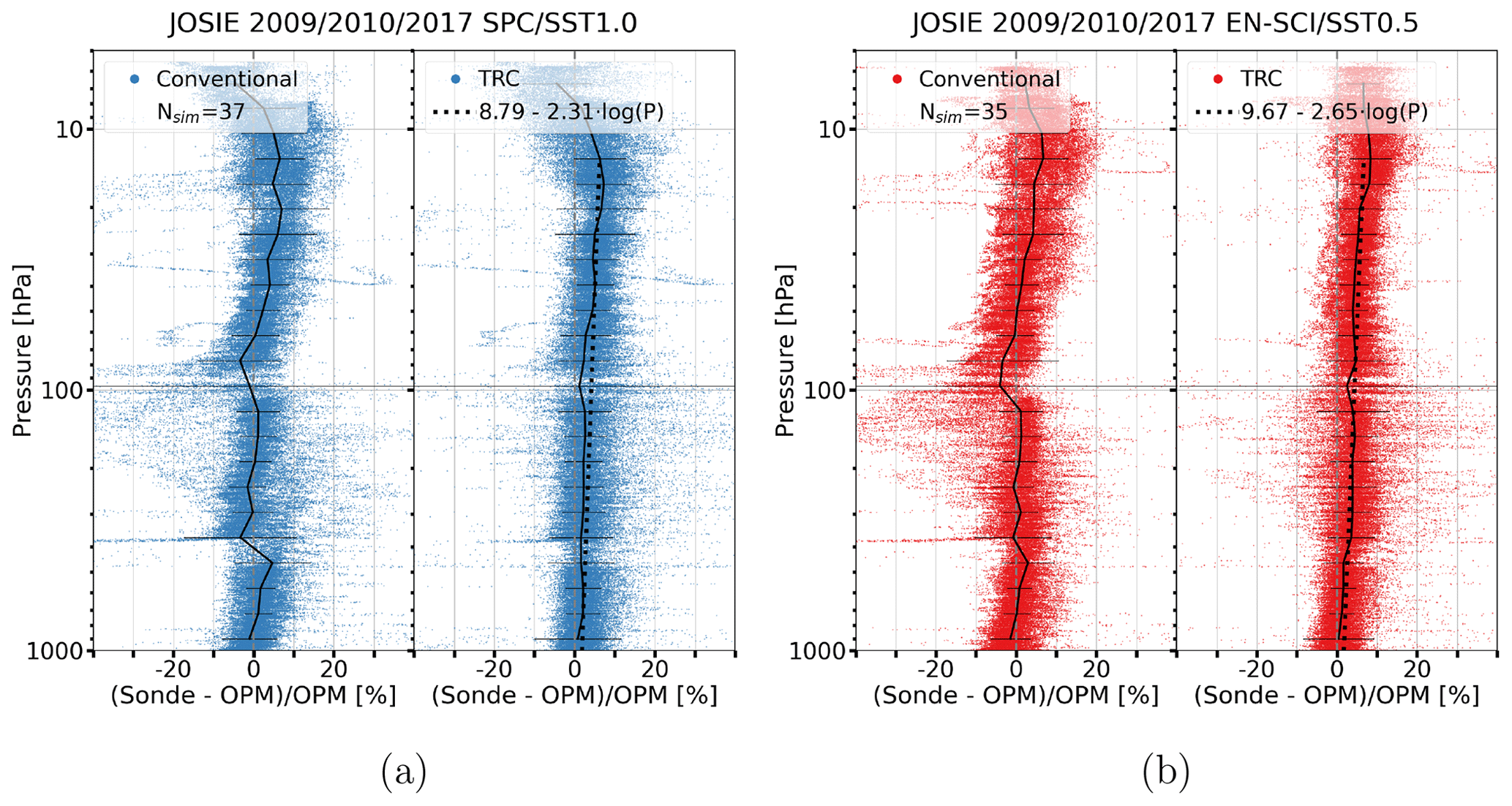
Figure 8JOSIE 2009/2010 and 2017: relative differences with the OPM for the conventionally processed (left part of each panel) and TRC-processed (right part of each panel) ozonesonde profiles for two pairs of sonde type and SST shown as scatterplots for SPC6A–SST1.0 (a, blue dots) and EN-SCI–SST0.5 (b, red dots). In each diagram for both methods, the mean and 1σ standard deviation are included (solid black line). The dashed black lines in the TRC diagrams are the linear regressions of the differences of the ozonesonde from the OPM as a function of the pressure (on a 10log scale).
The results of the parameterization of ηC(P), i.e. the offset a and the slope b (Eq. 18), including their uncertainties Δa and the slope Δb, respectively, are listed for the different pairs of sonde type and SSTs in JOSIE (2009/2010 + 2017) in Table 4. The sonde–SST pairs operated with SST0.5 and SST1.0 cover mid-latitude as well as tropical ozone profile conditions; i.e. the resulting ηC(P) functions are independent of the ozone profile. Based on this, we expect that ηC(P) for SST0.1, which could only be derived in this study for the tropical JOSIE 2017 conditions, can also be applied to non-tropical ozone profiles. Likewise, we expect that ηC(P) determined from JOSIE 2009 only for the SPC–SST0.5 and EN-SCI–SST1.0 pairs are valid for tropical ozone profiles. Of course, the derived linear regression coefficients for the calibration functions are directly linked to the pump efficiency values used, and it is assumed here that the average pump efficiency values used from Nakano and Morofuji (2023) in Table 1 are correct within their uncertainties and are representative of this study. However, if these pump efficiency values might change over time (see Nakano and Morofuji, 2023), the calibration functions must be adjusted accordingly.
Table 4Parameterization (offset a and slope b) of the calibrated conversion efficiency ηC(P) (Eq. 18) for the different pairs of SPC-6A or EN-SCI with SST1.0, SST0.5, or SST0.1 derived from the results of JOSIE 2009/2010 and JOSIE 2017. Included are the 1σ uncertainties Δa and Δb of the offset a and slope b in Eq. (18), respectively. The parameterization of ηC(P) is valid from P=1000 hPa until P=13 hPa (Z≈30 km) for SPC and for EN-SCI to 10 hPa (Z≈32 to 33 km).
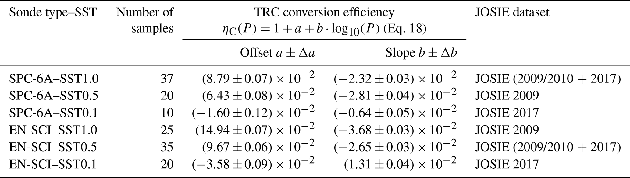
The calibration functions are presented here (Table 4) as a function of pressure, but this does not mean that they are really pressure-dependent. However, the goal is to provide a practical empirical representation of the overall performance of the ozonesonde, ascending with a balloon at ∼5 m s−1. The calibration functions can thus be interpreted as the correction term of the overall conversion efficiency of the ECC sonde when deviating from 1, but their origin is still unclear. Most likely this term relates to the unknown stoichiometry of the fast chemical reactions converting ozone into free iodine, in other words, the fast ECC current IF. This is supported by the shape of the vertical profiles of the absolute differences in the ECC sonde compared to the OPM for the TRC method, shown for the JOSIE 2009/2010, JOSIE 2017 and JOSIE 1996–2002 data (described in Sect. 5.3), in the middle diagrams of Figs. S3, S5 and S7, respectively. Indeed, in the middle stratosphere, the shapes of the residual currents compared to the OPM are more or less in phase with the simulated ozone profiles. This is most pronounced for the JOSIE 2017 tropical profiles (Fig. S5) and might indicate that these residual currents result from the fast chemical conversion and not from the 25 min delayed slow reaction. In the latter case, a phase shift between the residual currents and the ozone profile would be expected. The observed increase with altitude of typically 3 %–7 % in the calibration functions (Tables 3 and 4) might be explained by a small slightly increasing change in the stoichiometry of the fast O3 conversion due to an increase in KI concentration and buffer strength caused by evaporation during the sounding.
Although the cell temperatures of the ozonesondes (both SPC6A–SST1.0 and EN-SCI–SST0.5) in JOSIE 2009/2010 were about 10 ∘C higher than in JOSIE 2017, there are no direct indications that there is any cell temperature dependence of the calibration functions. This is demonstrated by the fact that SPC6A–SST1.0 and EN-SCI–SST0.5 for both campaigns show very similar OPM deviations over the course of the sounding when compared at the intercept points at P=1000 and 10 hPa (Table 3). However, temperature dependence cannot be completely excluded, in as much as the chemical reactions involved in the KI+O3 chemistry may have significant temperature dependencies. Again, further in-depth investigations are needed.
5.3 Application to JOSIE 1996 + 1998 + 2000 + 2002 data
The calibrated ηC(P) functions derived from JOSIE 2009/2010 and JOSIE 2017 (Table 4) for the different sonde–SST pairs are applied to TRC-processed ozonesonde data of JOSIE 1996 + 1998 + 2000 + 2002, in Fig. 9, again as relative differences from the OPM. In the remainder of this paper, we will use the abbreviation TRCC to denote that the TRC method has been applied with additional application of the calibration functions. The JOSIE 1996 + 1998 + 2000 datasets and results were described in detail by Smit and Kley (1998) and Smit and Sträter (2004a, b) and analysed by Smit et al. (2007). For JOSIE 1996, we excluded data from two participating laboratories (i.e. NOAA and CNRS) because their operating procedures deviated too greatly from the Komhyr (1986) procedures; JOSIE 2002 was a small campaign in which only three simulation runs were made with 10 SPC–SST1.0 sondes. The setup of the earlier campaigns was similar to the JOSIE 2009/2010 or JOSIE 2017 experiments. In the earlier campaigns mostly mid-latitude ozone profiles were simulated with the same four combinations of EN-SCI or SPC with either SST0.5 or SST1.0 (although the sample sizes with SST0.5 were rather small). The largest difference between JOSIE 2009/2010 and the early JOSIE campaigns lies in the preparation of the ozonesondes: in JOSIE 2009/2010, the same SOPs were followed by the three operators; ozonesondes “flown” in the earlier JOSIE campaigns were prepared by different teams of people with a variety of SOPs.
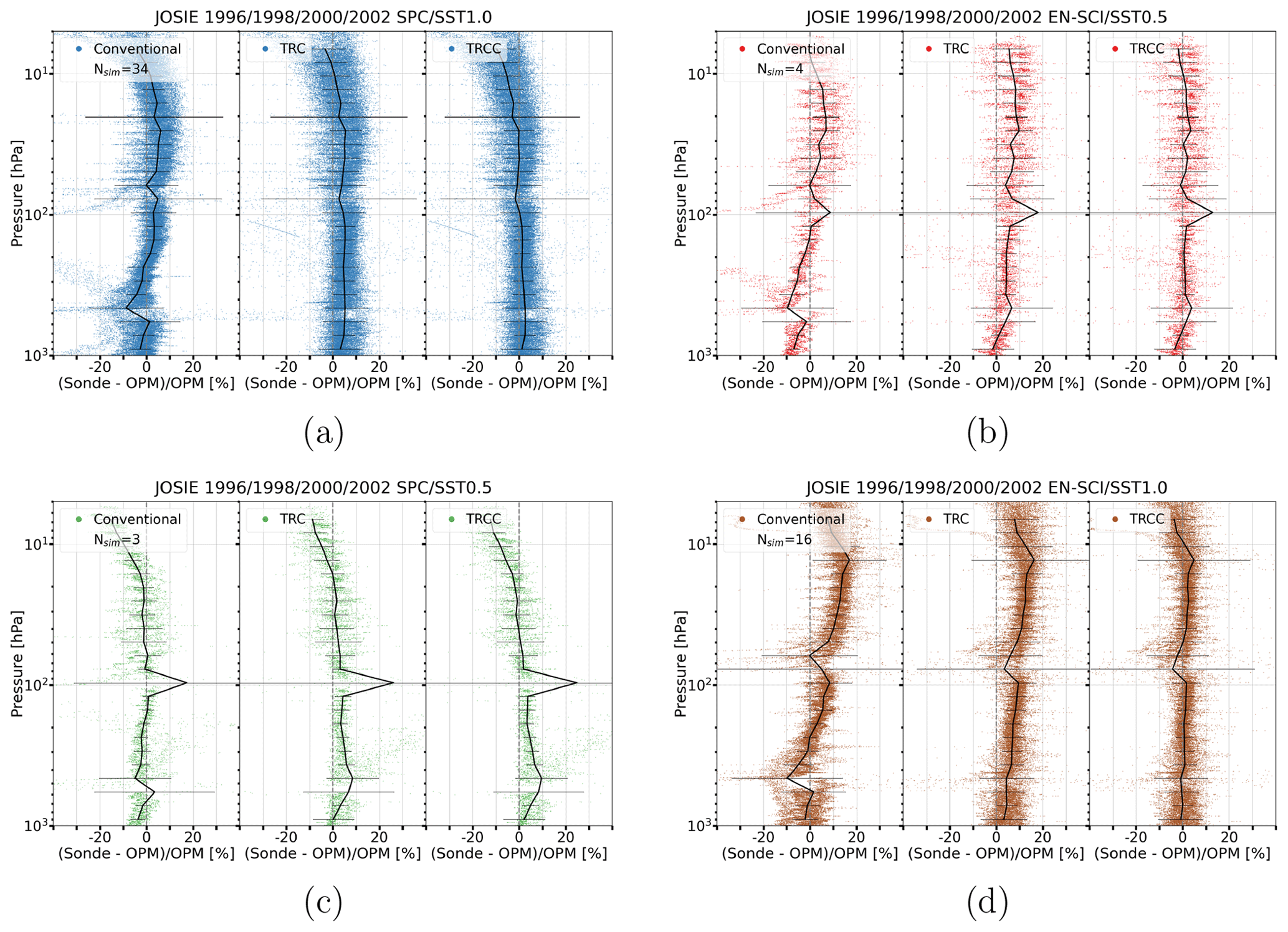
Figure 9JOSIE 1996 + 1998 + 2000 + 2002: relative differences [%] with the OPM for the conventionally processed (left part of each panel), TRC-processed (middle part of each panel) and TRCC-processed (TRCC denotes TRC + the application of calibration functions) (right part of each panel) ozonesonde profiles for four pairs of sonde type and SST, shown as scatterplots in four different colours in panels (a)–(d): SPC6A–SST1.0 (a, blue dots), EN-SCI–SST0.5 (b, red dots), SPC6A–SST0.5 (c, green dots) and EN-SCI–SST1.0 (d, brown dots), respectively. In each diagram for both methods the mean and 1σ standard deviation of the relative differences are included (solid black line). The absolute difference plots are available in the Supplement (Fig. S7), and in Fig. S8 is a summary plot of the relative differences.
The comparisons with the OPM in Fig. 9 are displayed for the TRC results, and are hence not calibrated (ηC(P)=1.00, middle panels), and for the TRCC corrections, i.e. calibrated (ηC(P) from Table 4, right panels), while the results for the conventional method (left panels) are also included. From the figure it is obvious that independent of the sonde type (SPC-6A or EN-SCI) or sensing solution type (SST1.0 or SST0.5), after applying ηC(P) the residual average curves (solid black lines) are within less than ±1 % deviation of the zero over the entire vertical profile until 7–10 hPa. This means that with the TRCC method, i.e TRC combined with the use of the specific ηC(P) for the various sonde–SST pairs, there are no longer systematic bias effects in the measured vertical ozonesonde profiles with respect to the OPM as a function of pressure (i.e. altitude). The use of the TRCC method can be a powerful tool to homogenize long-term ozone records in the global ozonesonde network so that these are now traceable to one reference standard, i.e. the OPM at WCCOS. The application of the TRCC method with the use of the calibration functions to the JOSIE 2009/2010 and JOSIE 2017 datasets is also illustrated in Figs. S3 and S5, showing the vertical profiles of the absolute differences of the sondes from the OPM for the conventional method, TRC and TRCC. This information is also provided for the absolute differences for the early JOSIE campaigns in Fig. S7.
In this section we quantify the impact of the individual corrections made in the TRCC method and estimate their uncertainty contributions to the overall uncertainty in the ozone partial pressure derived from the measured ECC ozone sensor current.
6.1 Contribution of correction steps of the TRC method for mid-latitude and tropical conditions
To derive from the measured cell current IM the partial ozone pressure in the ambient air, the TRCC method includes five different corrections: (i) constant background current IB0, (ii) slow cell current IS, (iii) time lag of fast current IF: deconvolved fast cell current (including smoothing), (iv) true pump efficiency (Nakano and Morofuji, 2023) and (v) calibrated conversion efficiency ηC(P) (Eq. 18 and Table 4). The impact of the different corrections on the measured cell current as a function of pressure (i.e. log10(P)) is shown in Fig. 10 for mid-latitude (JOSIE 2009/2010) and tropical (JOSIE 2017) vertical profile conditions for the standard sonde type–SST pairs, SPC6A–SST1.0 and EN-SCI–SST0.5, respectively; included are in addition examples of the different corrections made using the conventional method for JOSIE 2009/2010 and JOSIE 2017.
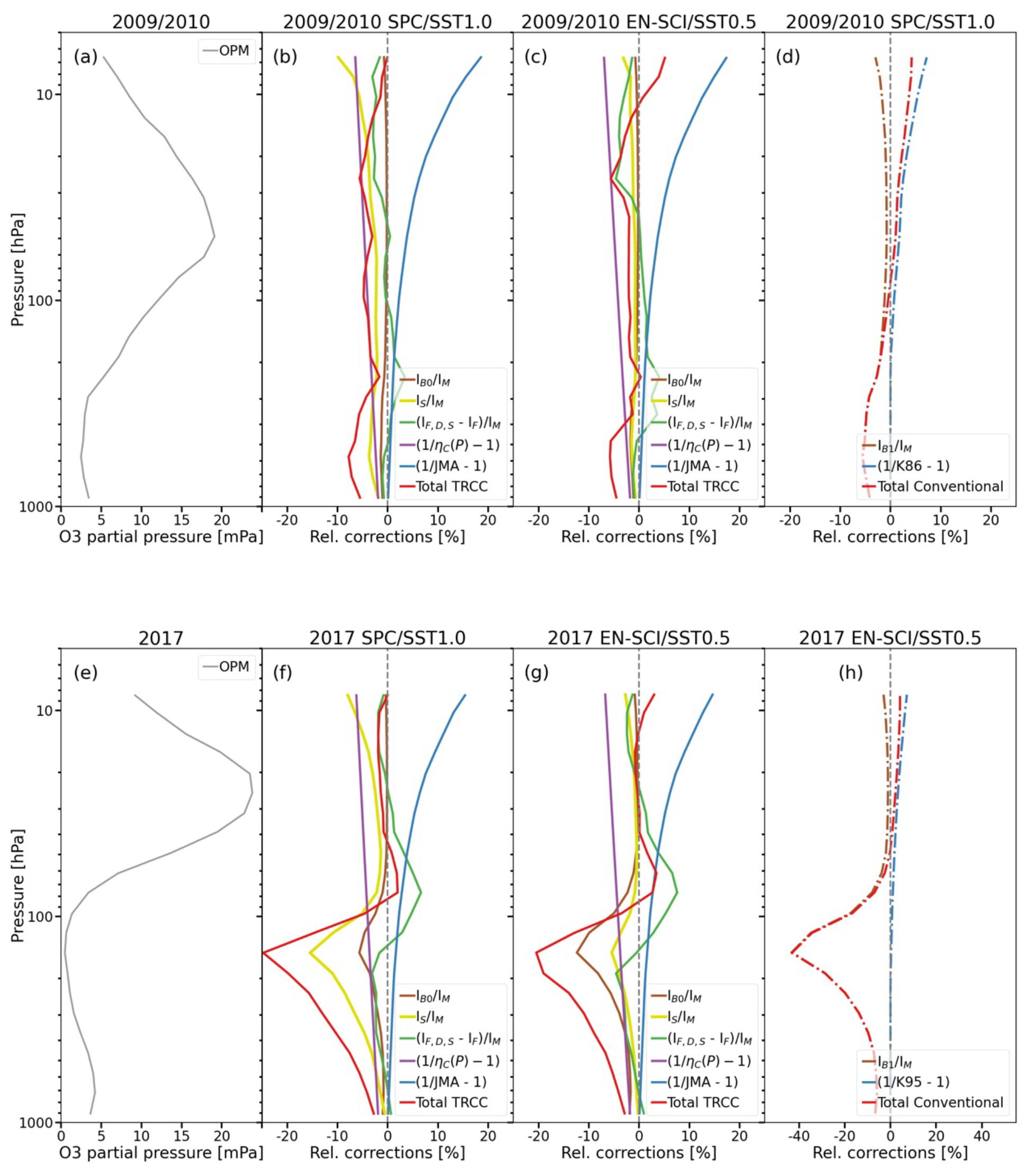
Figure 10Relative corrections of the TRCC method for typical mid-latitude (a–c: JOSIE 2009/2010) and tropical (e–g: JOSIE 2017) ozonesonde profiles, showing the influence of the different correction steps for the new TRCC method for SPC–SST1.0 (b and f) and EN-SCI–SST0.5 (c and g). The total correction (red line) consists of (i) IB0 (brown line), (ii) IS (yellow line), (iii) the deconvolved and smoothed IF (green line), (iv) the true pump efficiency (blue line – Nakano and Morofuji, 2023), and (v) the calibrated conversion efficiency (purple line). Panels (d) and (h) show the relative corrections of the conventional method for JOSIE 2009/2010 (SPC–SST1.0) and JOSIE 2017 (EN-SCI–SST0.5), respectively; the total correction (red line) consists of (i) IB1 (brown line) and (ii) the empirical effective efficiency (blue line – Komhyr (1986) for SPC and Komhyr et al. (1995) for EN-SCI, respectively).
A first, obvious, observation to make is that the corrections for a decreasing pump efficiency are identical for all sonde type–SST pairs and at pressures smaller than 100 hPa increase slowly but significantly from 1 % at P=100 hPa to 12 % at P=10 hPa and to almost 20 % at P=5 hPa. In the upper part of the profile (above 25 hPa), the decreasing pump efficiency is the dominating factor to correct for. In the lower part, below 100 hPa, the constant background IB0 (brown line) and the past ozone-dependent slow cell current Is (yellow line) are the major corrections, particularly in the upper tropical troposphere, with its very low ozone concentrations (panels f and g). Here, those corrections can amount to about 10 %–15 %, depending on, for example, the amplitude of the measured IB0 values. In this context, we also note that, because of the larger SS values for SPC6A–SST1.0, the past ozone-dependent slow-current (IS) correction will be larger by about a factor of 2 than the IS correction for EN-SCI–SST0.5 in all panels of Fig. 10. On top of this effect, for SPC6A–SST1.0 JOSIE 2009/2010 (Fig. 10b), above 10 hPa, the relative IS correction is even rapidly increasing in absolute value due to the limited performance of the SPC6A sonde in turn due to substantial losses of the sensing solution caused by boiling effects, as explained in Sect. 4.2. The impact of the time lag correction of the fast current is of the order of ±5 % and of course strongly dependent on the local vertical ozone gradient. Therefore, it can even become the dominant correction in the tropical upper troposphere–lower stratosphere (UTLS) region (between 5 % and 10 %), with its strong vertical ozone gradient (panels f and g). Finally, we mention that very similar results are obtained for the ozonesonde types combined with SST0.1, which are shown in the Supplement (Fig. S9).
All individual corrections of the TRCC method are based on known physical and chemical processes, with one exception being the remaining conversion efficiency, which was derived from calibration of the TRC-corrected probe readings with the OPM reference instrument. This contrasts with the corrections made in the conventional method (Fig. 10d and h), which were empirically derived to achieve a total ozone normalization factor close to 1. Therefore, the following corrections are applied: (i) an empirical effective efficiency function (Fig. 10, dashed blue line in graphs d and h) that represents the estimation of a decreasing pump efficiency and an increasing conversion efficiency (i.e. increasing stoichiometry of O3+KI redox reaction, Reaction R1, at lower pressures) and (ii) a background current IB1 correction that compensates for excessive ozone levels near the surface. However, in the tropics the IB1 correction is too large (Fig. 10h, dashed brown line) and leads to ozonesonde values in the troposphere that are significantly too low (Fig. S6a).
6.2 Uncertainty budget of the TRC method
For the conventional method, a detailed uncertainty budget has been studied by Tarasick et al. (2021) and described in detail in Smit et al. (2021) (Eq. E-3-1), together with practical guidelines to determine the overall uncertainty from the individual instrumental and procedural contributions. It is assumed that the uncertainties are random, uncorrelated and normally distributed and follow Gaussian statistics. In the case of the TRCC method, the overall relative uncertainty in is derived from Eq. (6), which has slightly changed compared to formula E-3-1 in Smit et al. (2021) as follows:
The additional term εi represents additional random uncertainties (Tarasick et al., 2021); in the case of the TRCC method, these can be, for example, the relative uncertainty contributions by the numerical schemes used of either the convolution to obtain IS(t) or the deconvolution of IF(t) and its additional smoothing.
To determine the uncertainty budget for TRCC in Eq. (19), the uncertainty contributions ΔηP, ΔηA, ΔIM, ΔIB0, ΔTP and ΔΦP0 are exactly the same as in Smit et al. (2021) following the guidelines in their Annex-C. However, the steps to determine the uncertainty contributions of the time-varying IF(t) and the pressure-dependent ηC(P) (see Table 4) differ from Smit et al. (2021), as detailed in the following subsections.
6.2.1 Uncertainty contribution ΔIF
From Eq. (7) the relative uncertainty in the fast sensor current IF(t) can be derived:
Here ΔIB0≈0.01 µA, obtained from the IB0 time series from Uccle. IS(t) estimations by varying the slow time constant with min have shown that ΔτS only has a minor contribution to ΔIS(t) of less than 1 %, while a potential contribution of the numerical convolution scheme itself is vanishingly small. It is obvious that ΔIS(t) is predominantly determined by the uncertainty ΔSS of the stoichiometry SS of the slow reaction path (Table 2) as
The impact of the slow time constant τS on the stoichiometry SS and its uncertainty ΔSS is also insignificant, as we assessed by varying min. Further, any contribution of the numerical scheme of deconvolution and its additional smoothing to the uncertainty in IF have been checked and appear to be vanishingly small (<0.5 %).
6.2.2 Uncertainty contribution ΔηC
The conversion efficiency ηC(P) (Eq. 18) has been calibrated to the OPM such that its uncertainty ΔηC(P) also includes the uncertainty in the measurement by the OPM as follows:
Hereby is the relative uncertainty in the measurement of the OPM, which is estimated to be better than 2 % at P>10 hPa and with lower pressures slightly increases to 3 % until P=5 hPa through potential small wall losses at these pressures. The reported relative uncertainty values here for the OPM are about 1.5 % better than the values mentioned before by Proffitt and McLaughlin (1983) because of the uncertainty in the new UV-absorption cross-section that is 7 times smaller (Hodges et al., 2019) compared to the former cross-section (Hearn et al., 1961) that was used before to derive the measurement of the OPM.
The overall uncertainty budget for the TRCC method is summarized in Table 5. Figure 11 shows the contributions of the different uncertainty sources to the uncertainty budgets for SPC6A–SST1.0 and EN-SCI–SST0.5 when applying the TRCC method for a typical mid-latitude and tropical ozone profile as used in JOSIE 2009/2010 and JOSIE 2017, respectively. The results for SPC6A–SST0.5 and EN-SCI–SST1.0 for JOSIE 2009/2010 and the low buffered SPC6A–SST0.1 and EN-SCI–SST0.1 for JOSIE 2017 are shown in Fig. S10. For the sake of clarity, the uncertainty contributions due to (i) ascent rate variation, (ii) pressure uncertainty and (iii) the total ozone normalization factor are not included here, as these are beyond the scope of this study. However, the characteristics of these uncertainty contributions, as reported by Tarasick et al. (2021) and Smit et al. (2021), would not change the uncertainty budget of the TRC method itself.
Table 5Sources of ozonesonde profile uncertainty and their estimated magnitudes for the TRCC method. All quoted uncertainties are 1 standard deviation (1σ).
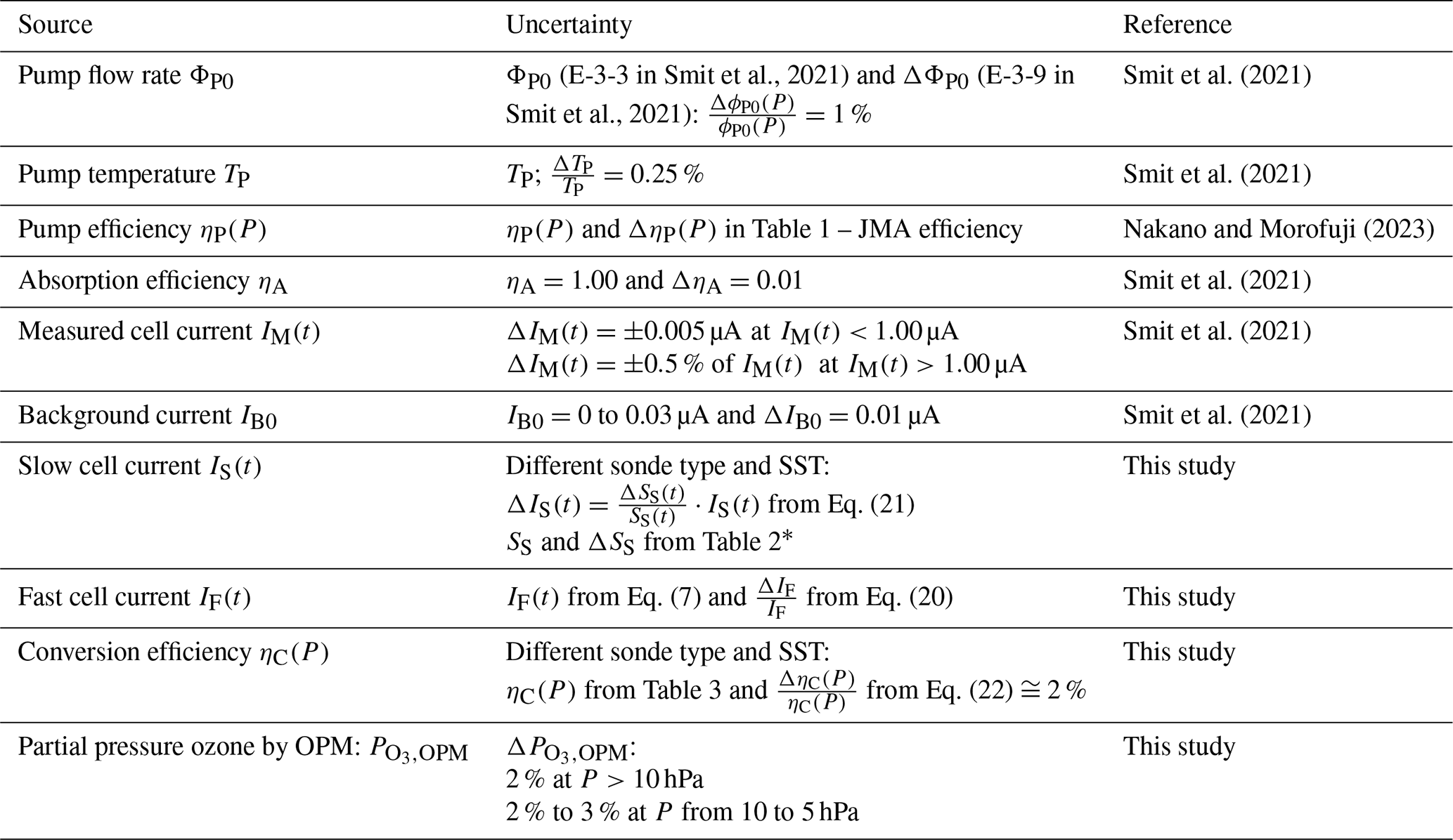
∗ To approximate ΔSS as a 1 standard deviation uncertainty, the MAD values (only covering 25th–75th percentiles) in Table 2 have been multiplied by 1.5 to become compatible with the Gaussian error propagation applied here.
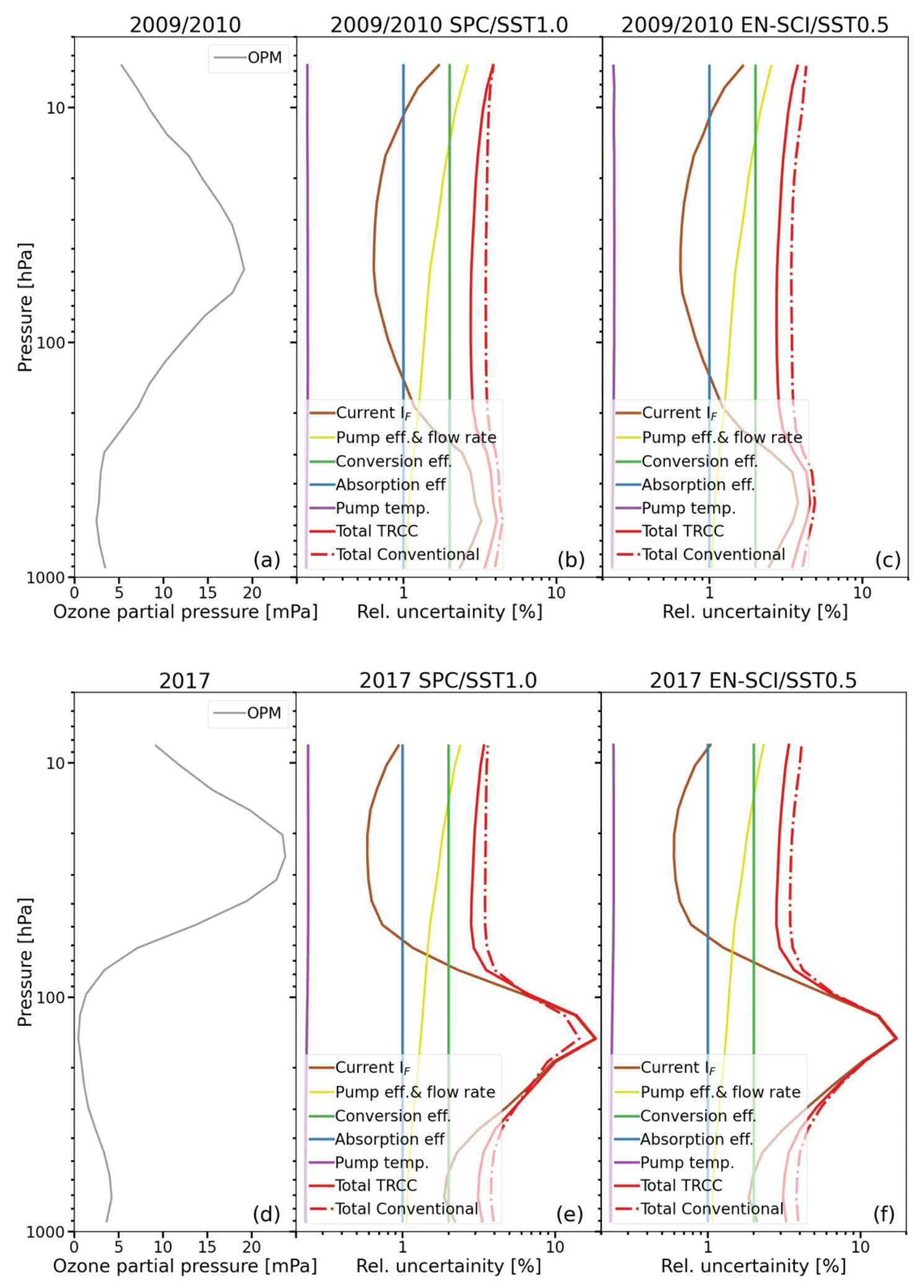
Figure 11Uncertainty budgets of a mid-latitude (panels a–c: JOSIE 2009/2010) and tropical (panels d–f: JOSIE 2017) ozonesonde profile, showing the influence of the different uncertainty source terms listed in Table 5 for the TRCC method for SPC–SST1.0 (panels b and e) and EN-SCI–SST0.5 (panels c and f). Total uncertainty (solid red line) consists of (i) the corrected cell current (brown line: ΔIFDS (TRC)), (ii) the pump efficiency and flow rate (yellow line: Δηc(P) and ΔΦP0), (iii) the absorption efficiency (blue line: ΔηA,), (iv) the conversion efficiency (green line: Δηc(P)), and (v) pump temperature (purple line: ΔTP). In addition, the total uncertainty in the conventional method is shown by the dashed red line.
In both the mid-latitude and tropical case (Fig. 11), it is seen that the (background) current in the troposphere and the conversion efficiency in the stratosphere are the dominant uncertainty sources. For the conventional method the conversion efficiency assumes that the overall stoichiometry factor is 1.00 with an uncertainty of 0.03 (Dietz et al., 1973) and is obviously also the dominant uncertainty source in the stratosphere. However, in this study we have shown that the overall stoichiometry can significantly differ from unity, which makes the overall uncertainty for the conventional method rather optimistic. For the TRCC method ΔηC(P) is mostly determined by the 2 %–3 % uncertainty in the OPM as the reference to obtain the ηC(P) calibration functions (Table 4). In the troposphere, the contribution of IS correction in the TRCC method is mostly smaller than the IB1 correction in the conventional method, particularly in the tropics.
However, both their contributions to the uncertainty are of the order of 0.01–0.02 µA, although on a relative scale they become strongly dependent on the magnitude of the ozone partial pressures, particularly in the upper tropical troposphere. In the stratosphere the contributions of the different uncertainties do not vary much, and the overall uncertainty stays well below 5 %.
It is to be noted that in the remote tropics in the upper troposphere the partial pressure of ozone can be very low, of the order of 0.1–0.3 mPa, while the detection limit of the ECC sensor is of the order of 0.01–0.02 µA, which corresponds to ozone levels of about 0.04–0.08 mPa. It is obvious that at these very low ozone levels the ECC sonde performance is strongly determined by its detection limit, which of course can have a significant and large impact on the overall uncertainty in the ozonesonde measurements.
A detailed procedure for applying the TRCC method in practice is described in Appendix C. In this section, we apply the methodology developed in the previous sections to ozonesonde profile data from three different stations: (i) a mid-latitude site (Uccle), (ii) a tropical station (American Samoa) and (iii) an ozone hole profile from the South Pole station in the Antarctic. At those sites, we selected ascent profiles and the corresponding descent profiles such that the methodology to resolve time response effects in the ECC signal can be assessed by comparing the ascent and descent profile of the same flight.
For the ozonesonde profiles of the three stations, we first determined the slow component IS(t) by convolution of the measured cell current IM(t) with an exponential decay with a time constant τS=25 min (Eq. 10) and conversion efficiencies SS=0.018 for SST0.5 (Uccle) and SS=0.023 for SST0.1 (Samoa and South Pole). For the IS at time t=0 of the launch, (i) zero is used at Uccle, as the last exposure to ozone usually occurs at least 1 h prior to launch and the measured value will fall back to IB0, and (ii) we use IB1−IB0 multiplied by the exponential decay factor , for the other two stations, with τs=25 min and Δt=30 min (South Pole) and 90 min (Samoa). Those time intervals are the typical time differences between the IB1 measurement and launch time at those sites. This slow component is then subtracted from the measured cell current IM, together with the background current IB0. The remaining signal is the fast component, which is deconvolved to correct for the fast time response τF. For the latter, the time lag measurements before launch at the stations (e.g. time to drop from 4 to 1.5 µA) are taken. The smoothing of IF,D is done by applying a Gaussian filter prior to the time lag correction using a width equal to 20 % of the fast time lag constant (as in Vömel et al., 2020). The final currents are then converted to ozone partial pressures using the calibration functions in Table 4 as the conversion efficiency, taking the Nakano and Morofuji (2023) true pump efficiency correction factors into account and correcting the pump temperature and the pump flow rates as in Smit et al. (2021). For the conventional method, the GAW recommendations have been followed rigorously, instead of subtracting IB0 (Uccle) and IB2 (Samoa and South Pole) as background currents.
In Fig. 12, the profiles corrected with the conventional method are on the left side, while the implementation of the TRCC method on the profiles is shown on the right side. It should immediately strike the eye that the agreement between the ascent and descent profiles is much improved after applying in particular the fast time response deconvolution with the new method, and this is the case for the three different sites. But the profile shapes, e.g. around the ozone peak maximum of the Uccle and Samoa profiles, also correspond much better with each other for the ascent and descent profiles for the new method. The slow time response correction contributes to a certain extent as well to this better profile shape agreement.
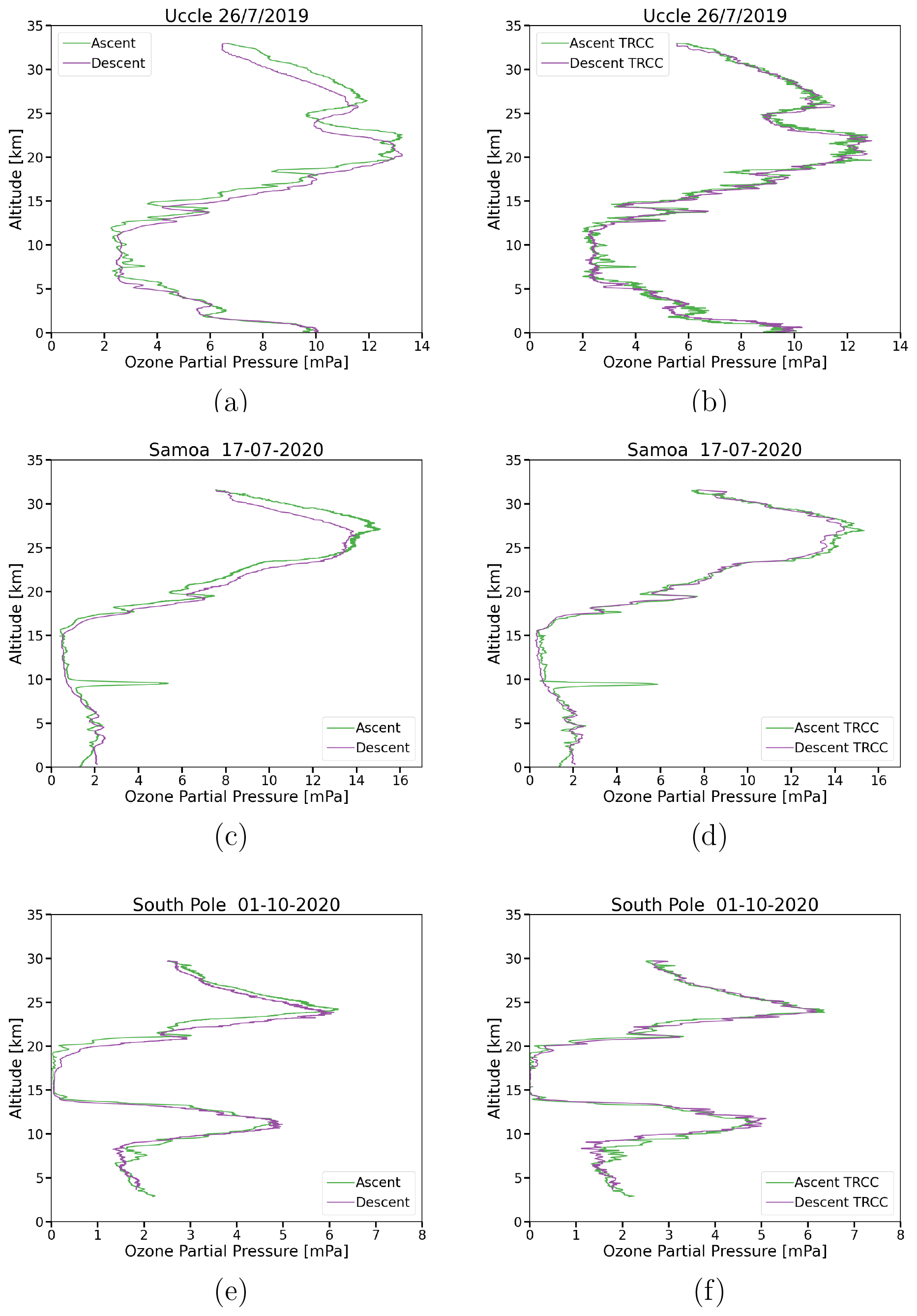
Figure 12Comparison of vertical ozone profiles obtained during ascent (solid green line) and descent (solid purple line) at three different ozone-sounding stations (Uccle, Samoa and South Pole) by applying the conventional method once (a, c, e) and the TRCC method (b, d, f).
The TRCC figures are remarkable in amplifying the features after correcting for the fast time constant. We already observed that the TRCC method is able to resolve some features in the ozonesonde data that were effectively present in the (faster) OPM ozone measurements in the JOSIE simulations. As mentioned by Vömel et al. (2020), the noise amplitude of the fast-response time-lag-corrected data is comparable to that of the original data, but its spectral characteristics are different because of the smoothing algorithm. As a result, individual data points are heavily influenced by the noise characteristics of the smoothed data. This is demonstrated by the ozone spike in the Samoa ascent, which has a larger peak amplitude for the TRCC method.
The ECC ozonesonde, in principle an absolute measuring device, encounters in the course of its flight several imperfections, e.g. changing pump and conversion efficiency, that need to be corrected for. In the actual processing chain, the “empirical effective efficiency” tables used (Komhyr, 1986; Komhyr et al., 1995) in fact represent an overall correction, empirically tweaked to coincident total ozone measurements, that includes both a measured pump flow efficiency and an estimate of the stoichiometry increase over the flight (Smit et al., 2021). However, the availability of recent measured true ECC pump flow efficiencies (Nakano and Morofuji, 2023), confirming earlier measurements, together with the knowledge that the ECC sonde response (chemical reaction pathways) is driven by a slow and fast component (Vömel et al., 2020; Tarasick et al., 2021), calls for a new approach. Vömel et al. (2020) also questioned the term background current in the ECC processing.
This study describes the concepts and the development of an updated methodology of ECC sonde data processing that applies a better correction of the ozone-exposure-dependent stoichiometry of the O3+KI titration reaction in the electrochemical cell of the ECC sonde using true pump efficiencies combined with resolving the time responses of the slow (≅25 min) and fast (≅20 to 25 s) components of the measured ECC ozone sensor current. Experimental evidence is given to treat the measured ECC sensor current as the superposition of a (i) dominant fast ozone current IF, (ii) slow time-variant current dependent on past ozone exposure IS and (iii) a constant ozone-independent background current IB0.
The time response correction plus calibration (TRCC) method developed here is briefly described in three steps:
- I.
The slow-cell-current component as a function of flight time is determined from the measured ozone sensor current, after correction for the constant background current IB0, using a first-order numerical convolution scheme (Eq. 10). Hereby, the in-flight time response tests of JOSIE 2009/2010 have been used to quantify the stoichiometry () factors SS (and their uncertainties) of the slow reaction pathways for both sonde types, SPC and EN-SCI, and two different sensing solution types, SST0.5 and SST1.0. In separate laboratory upward and downward response time experiments, SS and ΔSS of the low buffered combination of EN-SCI with SST0.1 have been determined using the same approach as in JOSIE 2009/2010 (see Appendix B). Depending on the buffer strength, the slow current typically amounts to about 1 %–4 % of measured cell current IM for SST0.5 or SST0.1 and about 2 %–8 % for SST1.0. However, in regions with very low ozone it can reach up to 10 %–15 %.
- II.
By subtracting the constant background current before exposure of ozone (IB0) and the time-variant slow sensor current IS from the measured ECC sensor current IM, the remaining fast sensor current IF has been resolved from the 20–30 s time response using a first-order deconvolution scheme (Eq. 12). Essential for this procedure is that the resulting deconvolved fast current IF,D has to be smoothed adequately to eliminate high-frequency noise.
- III.
From IF,D,S and using the correct true pump efficiencies (Table 1 – Nakano and Morofuji, 2023), the partial pressure of ozone measured by the ECC sonde is determined (Eq. 6). Additionally, using the conversion efficiency in Table 4 (“calibration functions”), the ozonesonde measurement is referred to the reference of the ozonesonde network, i.e. the photometer in the simulation chamber of WCCOS in Jülich.
Because the numerical convolution scheme used here is a recursive expression, the initial condition of IS at the launch carries the past ozone exposure of the pre-launch preparations. In laboratory experiments it was shown that after IB1 has been recorded during the pre-flight preparation, IS(t) will further decay exponentially at the slow time constant τS=25 min. Knowing the time span between recording of IB1 and turning on the pump just before launch IB1 can be used to derive the initial value of IS at the launch. Therefore, it is essential that during the pre-flight preparations background currents both before (IB0) and after (IB1) exposure of ozone are being recorded, including the time stamp at recording IB1 and activating the pump just before launch of the sonde. Similarly, our understanding of this slow time constant justifies the use of limiting values for IB0 and after IB1 in the operational preparation of ozone soundings (see Smit et al., 2021), with filters providing a good-quality zero-ozone air source.
The slow stoichiometry factor SS of the slow background due to the conversion of O3 into I2 and its median absolute deviation (MAD) uncertainties (Table 2) are each based on a statistically relevant number of samples. SS depends on the different SSTs used (Table 2) but is not dependent on the sonde type, which indicates that the secondary reaction pathway is not responsible for the systematic 4 %–5 % relative differences between EN-SCI and SPC when operating with the same SST. However, a direct quantitative relation of the buffer strength and the magnitude of SS only holds for the full buffered SST1.0 (SS≅0.046 to 0.050) and the half buffered SST0.5 (SS≅0.017 to 0.018) but not for the low th buffered SST0.1 (SS≅0.023). For SST0.1, significantly lower SS values might be expected, which might indicate that, in lower buffered sensing solutions, another competing chemical reaction scheme may occur that also produces free iodine at a 25 min timescale and contributes to IS. This may be the reason that, for not buffered or low buffered sensing solutions, IB1 values of 0.01–0.04 µA are still recorded.
SS values reported in Table 2 are significantly smaller than the so-called steady-state bias factor values applied by Vömel et al. (2020), which comprise the overall excess stoichiometry derived from steady-state experiments under ozone exposure (Vömel and Diaz, 2010). The difference may be explained by the overall excess stoichiometry originating from the secondary reaction pathway that only contributes partly to the slow IS while the other part still contributes to the fast IF (Appendix A). Further, in contrast to this study, Vömel et al. (2020) do not correct for IB0 before determining IS and calculating IF. These two different approaches in the methodology (e.g. IB0 subtraction and different stoichiometry factors Ss for the slow current IS) will of course lead to different results when comparing the sondes to the OPM. To demonstrate the impact of these different assumptions between both correction schemes, we have processed JOSIE 2009/2010 and JOSIE 2017 according to the TRC scheme used by Vömel et al. (2020). The comparisons are shown in the Supplement in Figs. S4 and S6 for JOSIE 2009/2010 and JOSIE 2017, respectively. The impact of subtracting IB0 is generally small and only significant in the upper troposphere in the tropics, where including subtraction of IB0 leads to better agreement with the OPM. The impact of larger SS values for SST1.0 and SST0.5 will lower the differences from the OPM above 100 hPa, but there still remains a significant deviation from the OPM. In the upper troposphere, the larger SS gives negative deviations, particularly in the tropics.
Different JOSIE datasets (JOSIE 2009/2010, JOSIE 2017 and JOSIE 1996 + 1998 + 2000 + 2002) have been used to compare the relative differences of the sonde from the OPM obtained with the time response correction (TRC) versus the conventional methodology of post-flight data processing (Smit and the ASOPOS Panel, 2014; Smit et al., 2021). Hereby, it is very important to mention that, in contrast to the conventional methodology, the relative differences obtained with TRC are almost independent of the ozone profile type (e.g. mid-latitude or tropical). In other words, the observed relative differences with TRC are independent of the past ozone exposure and increase only a few percent with altitude (or lower pressure). This is most pronounced in the tropical ozone profiles at 200–100 hPa pressure in the upper troposphere with very low ozone values and the steep vertical ozone gradient when entering the lower stratosphere. The typical systematic relative differences of 3 %–5 % for the same sonde type but different sensing solutions, SST1.0 or SST0.5, as observed since JOSIE 2000 are still preserved in the TRC method.
The different behaviour between JOSIE 2009/2010 and JOSIE 2017 regarding the relative differences in the TRC-corrected sonde profiles with the OPM for pressures smaller than about 13 hPa is ascribed to different pump temperatures used for the mid-latitude and tropical profiles in the respective campaigns. During JOSIE 2009/2010, the higher pump temperatures led to a higher boiling rate in this pressure range, confirmed by the higher solution weight losses.
The TRC mean relative differences in the sonde with the OPM show a strong consistency for the different pairs of sonde type and SST and can be therefore represented by a linear regression as a function of log10 of the pressure. This linear regression can be interpreted as the calibration function for the conversion efficiency, which is not quite equal to 1 (Eq. 18). The calibration functions introduced here for the various sonde–SST combinations, parameterized as a function of ambient air pressure in Table 4, are independent of the ozone exposure and thus invariant to the measured ozone profile itself. The use of these calibration functions makes the global ozonesonde records traceable to one common standard, i.e. the OPM of WCCOS. The origin of these calibration functions remains speculative, but there are some experimental indications that they are linked to the unknown stoichiometry of the fast chemical conversion of O3 into I2 and not caused by an underestimation of the slow cell current IS. It is to be noted that the calibration functions reported here are directly linked to the average pump efficiency values from Nakano and Morofuji (2023) as in Table 1; however, if these pump efficiency values might change over time (see Nakano and Morofuji, 2023), the calibration functions must be adjusted accordingly.
The overall uncertainty in combining the TRC method with the calibration functions (TRCC) is about 3 %–4 % throughout the entire ozone profile, except for the upper troposphere, where the overall uncertainty can increase to up to 10 % for very low ozone amounts, particularly in the tropics. The major uncertainty sources in the upper troposphere are the constant background current IB0 and the slow current IS (i.e. SS).
The TRCC method has been tested in practice (practical guidelines in Appendix C) for three different vertical ozone profiles measured during ascent and descent at a mid-latitude site and a tropical station and during an ozone hole at the South Pole. The resolving power of the fast-deconvolution numerical scheme is clearly demonstrated by removing the strong delay shift in the descent ozone profile compared with the ascent ozone profile before and after applying the TRCC method. However, the examples also clearly demonstrate the importance of careful and proper smoothing of the deconvolved ozone profile. To apply the TRCC method to the time series of an ozonesonde site, a proper determination of IB0 and IB1 is required. Imperfect or defective zero-ozone air filters might increase those background currents by several orders of magnitude, compromising the subtraction by the (too high an) IB0 value throughout the entire profile and at the beginning of the profile due to the high initial value for IS(t0). Some more analysis is needed to formulate alternative approaches for these cases. As also stated by ASOPOS 2.0 (Smit et al., 2021), the use of proper gas filters to provide ozone-free, dry and purified air in practice at the sounding site is essential not only in general but also when applying the TRCC data processing.
An important outcome of this study is also that the contribution of the slow current IS is not as large as previously thought (Vömel et al., 2020) because TRC demonstrates that the secondary pathway involving the buffer can also contribute to the fast stoichiometry factor to increase the fast current IF so that the uncalibrated conversion efficiency exceeds 1, which is most likely the case for SST1.0 and SST0.5. This is in contrast to SST0.1, where the slow current has most likely a different chemical origin and not an additional contribution to IF, so the fast stoichiometry (i.e. conversion efficiency) does not exceed 1 and is even a few percent lower. The underlying chemical mechanisms remain speculative in some cases, and the stoichiometry of the fast O3+KI chemistry cannot be quantified explicitly but only expressed implicitly in the conversion efficiency with the introduction of calibration functions (Table 4). These calibration functions can improve the homogenization of long-term ozonesonde records of the global network, making the data traceable to one ozone standard, the OPM at WCCOS at Jülich (Germany). Our OPM reference values have been scaled up 1.23 % compared to earlier JOSIE publications because of the revised UV ozone absorption cross-section at 254 nm (BIPM, 2022; Hodges et al., 2019). The latter adjustment is being introduced into the global ozone network in 2024/2025.
Finally, we list some specific recommendations for further research as follows:
-
Regular JOSIE campaigns at WCCOS (Jülich, Germany) are essential to check the long-term stability of the calibration functions reported in this study (Table 4) and to guarantee the long-term traceability of global ozonesonde records to the OPM standard.
-
More research is needed to understand the slow stoichiometry SS factors in more detail, particularly for the low or not buffered sensing solutions for which the underlying chemical processes are not understood at all. A key question hereby is also the role of KBr in the sensing solutions. This should be in conjunction with understanding the differences observed between the methods to derive SS from either a zero-ozone or an ozone exposure time response experiment. Dedicated laboratory experiments in the WCCOS simulation chamber can accomplish this.
-
More detailed understanding is needed of the chemical reaction mechanisms that are responsible for the fast and slow cell current response of the ECC sensor, and their interaction. This should include determining the temperature dependency of the KI+O3 chemistry.
-
Better knowledge is needed of the time behaviour of the high background currents IB0 and IB1 that are often measured in practice at the sounding sites when not using proper gas filters. Experiments are necessary to describe and eventually correct for this high IB0 and IB1 caused by using inadequate gas filters. This is essential as reprocessing ozonesonde records often goes hand in hand with correcting very high IB0 and IB1.
This study did not solve the systematic 3 %–5 % offsets in measured ozone concentrations between EN-SCI and SPC instruments when operating with the same SST. However, we showed that the SS values are comparable for both sondes with the same SST, which means the differences are not caused by the slow chemistry. More research here is essential.
Both the TRCC method and the conventional method are post-flight data-processing methods that assume the following three basic QA criteria are met: (i) best operating practices at the ozone monitoring stations in the global network (Smit et al., 2021), (ii) high-quality balloon instruments (e.g. ozone and radiosondes) and ground equipment, and (iii) well-trained operators at the sounding site. Even small imperfections in these QA criteria can result in significant degradation in the quality of recorded ozonesonde data, such as the recently observed sudden drop in the total column ozone (TCO) measurements of ozonesondes compared to other TCO-measuring instruments (e.g. satellites) (Stauffer et al., 2020). Neither the TRCC method nor the conventional method can avoid these inconveniences. However, it highlights the future need for QA monitoring of ozonesonde data in quasi-real time and comparing them with satellite and ground-based (e.g. lidar or Dobson–Brewer) data to detect potential artefacts (e.g. Stauffer et al., 2022).
Iodometric determination of ozone and the underlying oxidation of iodide ions by ozone to liberate iodine have long been the subject of controversy. The reaction of KI with O3 may proceed through a variety of chemical pathways that strongly depend on pH and KI and O3 concentrations, whether or not in the presence of a pH buffer. In this study the focus is on the neutral buffered potassium iodide (NBKI) method and its application in the ECC ozone sensor. Experimentally it was shown by several investigators (e.g. Saltzman and Gilbert, 1959; Flamm and Anderson, 1975) that iodate () as an intermediate can be excluded as long as ozone partial pressures in the air are well below 100 mPa. This makes it most likely that much of the behaviour of the ECC and its slow and fast sensor currents may be explained by the chemical reaction mechanisms for NBKI and the impact of the phosphate buffer as postulated by Saltzman and Gilbert (1959). It was experimentally shown that the fast and slow reactions increase as KI concentrations increase, whereby the slow reactions increase with the buffer concentration. Buffered solutions with no KI show no evidence of gaseous O3 uptake into the sensing solution, indicating that the additional reactions with O3 are secondary reactions after the initial O3+KI reaction.
A1 Primary reaction pathway
In ion-notation, this is
Or in detail (postulated after Saltzman and Gilbert, 1959) it is
Losses of IO−, i.e. I2, are as follows:
-
If all O3 were absorbed and reacted with KI in this primary reaction pathway, it would be expected that the stoichiometry for , i.e. in neutral/acid solution, is equal to 1.
-
However, self-reaction of IO− (Reaction AR6) can be a loss mechanism, competing with the formation of I2 (Reaction AR4).
-
In general, loss mechanisms of IO− might compete with Reaction (AR4), and then the stoichiometry of the primary reaction pathway is less than 1.
-
The ECC shows for 1 % KI and no buffer a stoichiometry less than 1 (Johnson et al., 2002).
-
Dismutation (disproportioning) of IO− into iodate () and I− is extremely slow and is of no importance in the case of the ECC sensor. Iodate chemistry first plays a role at significantly higher KI or O3 concentrations than are used in the ECC sensor or encountered in the atmosphere, respectively.
A2 Secondary reaction pathway: impact of phosphate buffer
But losses of I2 iodine (via IO− losses) are also as follows:
-
Reaction (AR7) is the key reaction to form extra IO− that can react via Reaction (AR4) into I2 and contributes in addition to the fast reaction pathway and thus adds to the stoichiometry causing the fast ECC signal.
-
can be seen as the interim reactant that is formed fast but via Reaction (AR8) decays slowly to form extra IO−. This latter can produce in addition extra I2, which causes the slow part of the ECC current.
-
It is known that reacts similarly to H2O2 to form IO−, i.e. I2 with a typical time constant of about 25 min; this fits the slow, secondary response time of the ECC of typically 25 min.
As no time response tests are available during JOSIE campaigns for SST0.1 to determine SS, we undertook laboratory measurements under room conditions in Uccle (Belgium). During the experiments, four ozonesondes were simultaneously exposed to ozone amounts generated by a photometric ozone calibrator Teledyne API T703 according to the following scheme (three times): 30 min of exposure to a value of 450 µg m−3 (around 225 ppb) ozone was preceded and succeeded by 10 min of ozone-free air; see Fig. B1. The value of 450 µg m−3 has been imposed by the upper limit (6.5 µA) of the microcurrent meters used in the Forschungszentrum Jülich homemade ground calibration box for the four ozonesondes. These microcurrents were read out digitally, and, as in the JOSIE campaigns, the SS values were again estimated as the average over a 50 s time interval between 4 and 5 min after the end of the ozone exposure. As the time response test intervals in these laboratory measurements are twice as long (10 min) as in the JOSIE 2009/2010 campaigns, we tried different timings for the determination of the SS values, but they did not give significantly different results for the slow stoichiometry coefficients. Again, the differences between the SS values obtained from the different time response test intervals RT in one experiment were insignificant as well.
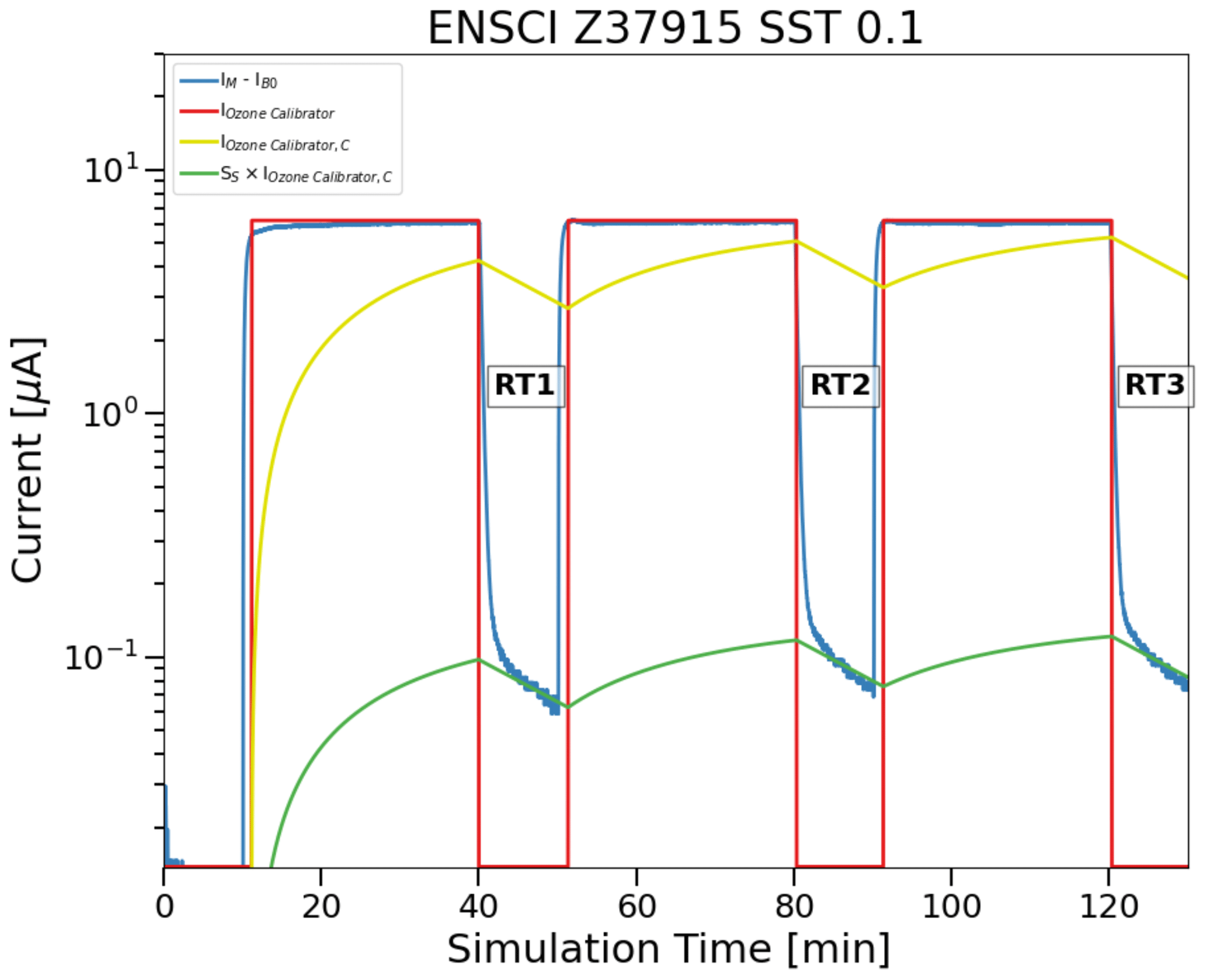
Figure B1Example of a series of three upward and downward ozone steps generated by a photometric ozone calibrator Teledyne API T703 (represented by the generic IOzone Calibrator: red line) and the response of the measured cell current IM−IB0 (blue line) of an EN-SCI–SST0.1 ozonesonde as a function of time, the 25 min convolved IOzone Calibrator, C (yellow line), and the slow current after determination and application of SS (SS×IOzone Calibrator, C: green line).
In total, we have eight SS estimations with four EN-SCI ozonesondes filled with SST0.1 solutions that come from three different experiment runs: two runs with each two (new) EN-SCI ozonesondes (with SST0.1) and a run with all four (re-used) EN-SCI ozonesondes involved. These four ozonesondes, all with serial numbers Z379xxx, have been prepared by the same person, according to the SOPs defined in Smit et al. (2021). The median value for SS for the eight experiments, each including three time intervals, is 0.023 ± 0.005. This value is very close to the value SS=0.017 found for SST0.5 during the JOSIE 2009/2010 campaign, whereas a smaller value could be expected due to the lower buffer amount in SST0.1 (see Johnson et al., 2002, and Sect. 3.2). However, the same Uccle experimental setup and method as described here above for EN-SCI–SST0.1 have been used to determine the SS coefficient for four EN-SCI ozonesondes filled with SST0.5 (serial numbers Z379xxx but different from those used with SST0.1) during two experimental runs. The resulting median value, 0.022 ± 0.004, is again in close agreement with the value determined for EN-SCI–SST0.5 with JOSIE 2009/2010 (0.018 ± 0.004), confirming the consistency between the two instrumental setups to determine the stoichiometry coefficients. Nevertheless, a JOSIE campaign is foreseen in 2024 to determine the SS factors for SST0.1 for both EN-SCI and SPC ozonesondes, using the same simulation setup as in JOSIE 2009/2010.
In this part of the Appendix, we give a schematic overview of the different steps that need to be taken to implement the TRCC method in the data processing of an ozonesonde time series in practice, displayed schematically in the flowchart in Fig. C1. First, it should be noted that the TRC method is applied to the currents measured by the ozonesonde. Hence, these ozonesonde's raw measurements should be available. Normally, when a site has been homogenized as part of the O3S-DQA activity, the currents have been made available or have been converted back from the ozone partial pressures. Secondly, the TRCC method demands the knowledge of some metadata parameters that should have been measured during the preparation of the ozonesonde 0–1 d prior to launch (see also Fig. C1): IB0; IB1; the time of the IB1 measurement (relative to the launch time); and the sensor fast response time τF, measured as the time to drop from 4.0 to 1.5 µA (after the 5 µA test). If those metadata parameters are missing, these might be estimated as the means over a representative time period, e.g. using the same filter for determining the background currents or the same batch of ozonesonde serial numbers or sensing solution for the fast response time.
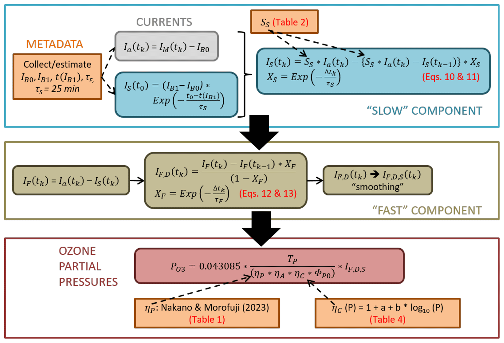
Figure C1Flowchart summarizing the processing steps for the time response correction and calibration (TRCC) method for correcting ozonesonde data. The table and equation numbers in red refer to those in this paper.
In a next step, the IB0 value is subtracted from the time series of measured currents of the sounding, resulting in Ia(tk), and all forthcoming calculations should be done with those currents Ia(tk). As the calculation for obtaining the slow component of the ECC signal is a recursive equation (Eq. 10), the slow component at launch time should be estimated first. Therefore, it suffices to start from the last measured value of the ozonesonde before launch, IB1, corrected for (i.e. subtract) the IB0 value, and convolve it with an exponential decay function with a slow time constant of 25 min. Hereby, the time difference between the IB1 measurement and the launch is used. If this time difference is large enough (Smit et al., 2021, recommend a minimum 30 min time window), the exponential decay function will be close to zero; IB1 will approach the IB0 value; and the slow component at launch time will be zero, which is the allowed lower limit. Now, for every time step, the slow component of the ECC signal can be calculated from Eqs. (10) and (11) using the stoichiometry factor SS from the sonde–SST combination (see Table 2). This slow component can be seen as a time-varying background current and should be subtracted from the currents Ia(tk), to be left over with the fast component IF of the ECC signal.
To eliminate the 20–25 s response delay in the fast component, the latter can be deconvolved (Eqs. 12 and 13), i.e. corrected for the exponential decay of the signal with the fast sensor response time, measured before launch. This deconvolution will introduce a lot of noise into the signal, and therefore, a smoothing of the current, either before or after the deconvolution, will be necessary. Different smoothing algorithms can be considered, with different filter widths and/or time windows (e.g. for running averages). The choice of the smoothing algorithm depends on the application, e.g. to resolve steep vertical gradients; on the profiles (smooth mid-latitude vs. upper-tropospheric tropical profile); and on the measurement time interval (10 s versus 1 s time resolution). In the end, a compromise between the smoothness of the profile and a full correction for the time response delay around strong vertical gradients should be sought.
The smoothed, deconvolved time series of the fast component IF,D,S of the ECC signal is then used in the basic equation of the ozonesonde signal, converting the current to ozone partial pressure. In this equation, the recommended corrections for TP, ηA and ϕP0 in Smit et al. (2021) should be implemented as well: the conversion to the piston pump temperature (E-3-15), a correction for the absorption efficiency if the cathode cell was only filled with 2.5 cm3 of solution before launch (E-3-11-A&B), and the humidification (E-3-4) and pump temperature (E-3-7) corrections for the pump flow rate at the ground. In comparison with the recommended processing in Smit et al. (2021), the true pump efficiency corrections proposed by Nakano and Morofuji (2023) should now be used for all combinations of sonde type and SST, as these are the actual measured ones. The Komhyr (1986) and Komhyr et al. (1995) tables should be discarded, as these are empirical effective efficiency curves and they actually combine pump efficiency and conversion efficiency. A last difference with the conventional method as proposed in Smit et al. (2021) is the use of the calibration functions defined in Sect. 6, Eq. (18): , with the coefficients a and b determined for every sonde type and SST combination separately (see Table 4), for the conversion efficiency, instead of adopting the value ηC(P)=1.00. Using the calibration functions, the ozone-sounding measurement should be traceable to the common reference of the ozonesonde network, the ozone photometer OPM in the simulation chamber of the World Calibration Centre for Ozone Sondes in Jülich.
To calculate the uncertainties associated with the ozone partial pressure measurements of an ozonesonde, corrected with TRCC, the uncertainty equation E-3-1 in Smit et al. (2021) forms the basis. With respect to this formula, the uncertainty equation for the TRC method (see also Fig. C2) has one changed term, and the meaning of a couple of other terms has changed. We will only describe these three terms here.
First, as both IB0 and the slow component IS are subtracted from the measurement background in the TRC method, the uncertainties in IB0 and IS should be included now. For IB0, the uncertainty is estimated to be 0.01 µA, and the (relative) uncertainty in the slow component is, in a first-order approximation, equal to the (relative) uncertainty in the stoichiometric coefficient SS. The uncertainties in SS for the different SSTs can be found in Table 2.
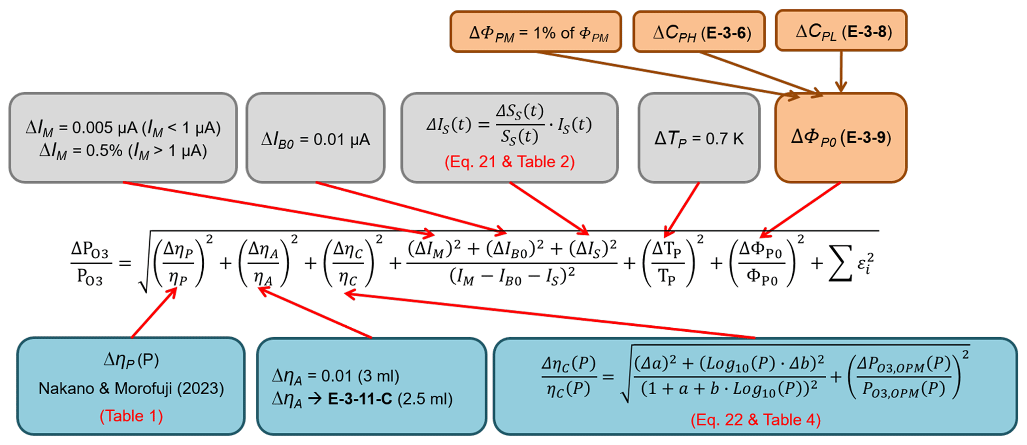
Figure C2Overview of the different data-processing steps and input to derive the uncertainty in the ozone partial pressure measured with an ozonesonde, using the TRCC method. Figure adapted from Fig. C-4 in Smit et al. (2021). The equation numbers also refer to equations in this GAW report. Table numbers in red refer to tables in the main text of this paper.
For TRCC, the uncertainties in the pump efficiencies ΔηP(P) are now equal to the standard deviations of the true pump efficiency measurements reported in Nakano and Morofuji (2023), also shown in Table 1. Finally, the uncertainty in the conversion efficiency is no longer estimated as a fixed value ΔηC(P)=0.03 but should take into account the uncertainty in the derived calibration functions in Sect. 6 (see Table 4 for the uncertainties in the linear regression coefficients a and b for the different combinations of sonde type and SST), as well as the uncertainty in the photometer (OPM) to which the ozonesonde measurements are traced back. This latter (relative) uncertainty is estimated to be around 2 %.
| IB0 | Background current before exposure with ozone (after 10 min flushing cathode cell with zero air) |
| IB1 | Background current after exposure with ozone (after 10 min flushing cathode cell with zero air) |
| IB2 | Background current at launch site just before flight |
| IB | Background current used in data processing in Eq. (1). |
| IM | Measured (cathode) cell current |
| IOPM | Ozone-equivalent ECC current at time t derived from OPM |
| IF | Fast cell current |
| IF,D | Fast cell current, deconvolved |
| IF,D,S | Fast cell current, deconvolved, smoothed |
| IS | Slow cell current |
| SF | Stoichiometry factor of fast reaction pathway of conversion of O3 into I2 |
| SS | Stoichiometry factor of slow reaction pathway of conversion of O3 into I2 |
| Ozone partial pressure | |
| R | Universal gas constant |
| F | Faraday constant |
| TP | Pump temperature |
| ΦP0 | Pump flow rate |
| ηA | Absorption efficiency |
| ηP | Pump efficiency |
| ηC | Conversion efficiency |
| ηT | Total (overall) efficiency |
| τF | Response time of fast reaction pathway of conversion of O3 into fast-cell-current component |
| τS | Response time of slow reaction pathway of conversion of O3 into slow-cell-current component |
| RT1, RT2, RT3, RT4 | Response time tests in vertical ozone profile |
| ASOPOS | Assessment of Standard Operating Procedures for Ozone Sondes |
| BESOS | Balloon Experiment on Standards for Ozonesondes |
| CMDL | Climate Monitoring and Diagnostics Laboratory (now GML) |
| ECC | Electrochemical concentration cell |
| EN-SCI | Environmental Science Corporation; ECC ozonesonde manufacturer |
| FZJ | Forschungszentrum Jülich |
| GAW | Global Atmosphere Watch |
| GML | Global Monitoring Laboratory (NOAA Earth System Research Laboratories) |
| H2O2 | Hydrogen peroxide |
| IAP | Institute of Atmospheric Physics, Beijing, China |
| IGACO | Integrated Global Atmospheric Chemistry Observations |
| IO3C | International Ozone Commission |
| IPCC | Intergovernmental Panel on Climate Change |
| JMA | Japanese Meteorological Agency |
| JOSIE | Jülich Ozone Sonde Intercomparison Experiment |
| KI | Potassium iodide |
| NASA | National Aeronautics and Space Administration |
| NBKI | Neutral buffered potassium iodide |
| NDACC | Network for the Detection of Atmospheric Composition Change |
| NOAA | National Oceanic and Atmospheric Administration |
| NOx | Nitrogen oxides |
| O3S-DQA | OzoneSonde Data Quality Assessment |
| OPM | Ozone photometer instrument (used as ozone UV photometer reference at WCCOS) |
| SHADOZ | Southern Hemisphere Additional Ozonesondes |
| SI2N | Ozone trend assessment study supported by SPARC, IO3C, IGACO, and NDACC |
| SOP | Standard operating procedure |
| SPARC | Stratosphere-troposphere Processes And their Role in Climate |
| SPC | Science Pump Corporation; ECC ozonesonde manufacturer |
| SST | Sensing solution type |
| SST0.1 | 1.0 % KI and th buffer solution |
| SST0.5 | 0.5 % KI and half-pH-buffer solution |
| SST1.0 | 1.0 % KI and full-pH-buffer solution |
| SST2.0 | 2.0 % KI and non-pH-buffer solution with no KBr |
| TRC | Time response correction |
| TRCC | TRC + calibration |
| UNEP | United Nations Environment Programme |
| UV | Ultraviolet |
| UWYO | University of Wyoming |
| VOC | Volatile organic compound |
| WCCOS | World Calibration Centre for Ozone Sondes |
| WMO | World Meteorological Organization |
| WOUDC | World Ozone and Ultraviolet Radiation Data Centre |
The software code can be provided by Roeland Van Malderen on request.
All the JOSIE data used in this study are available at https://doi.org/10.14287/100000014 (WOUDC data archive, 2023).
The supplement related to this article is available online at: https://doi.org/10.5194/amt-17-73-2024-supplement.
(i) The very first idea of resolving the slow and fast response times was proposed by DWT and the ASOPOS Panel; (ii) the concept of this study was developed and worked out by HGJS and RVM; (iii) data processing was by DP; (iv) data analysis was by HGJS, RVM and DP; (v) preparation of the manuscript was led by HGJS and RVM with the support of all co-authors. Data provision was by HGJS (JOSIE campaign data) and RVM (Uccle ground check and laboratory data).
At least one of the (co-)authors is a member of the editorial board of Atmospheric Measurement Techniques. The peer-review process was guided by an independent editor, and the authors also have no other competing interests to declare.
Publisher's note: Copernicus Publications remains neutral with regard to jurisdictional claims made in the text, published maps, institutional affiliations, or any other geographical representation in this paper. While Copernicus Publications makes every effort to include appropriate place names, the final responsibility lies with the authors.
This article is part of the special issue “Atmospheric ozone and related species in the early 2020s: latest results and trends (ACP/AMT inter-journal SI)”. It is not associated with a conference.
For JOSIE 2009/2010 we are very grateful to Marcel Berg (FZJ IEK-8, Germany) and Johannes Staufer (ETH Zürich, Switzerland) for the pre-flight preparation of the ozonesondes. Many thanks to Holger Vömel for stimulating discussions in preparing the manuscript. Also, many thanks to the people who supplied ECC sondes to be flown in the simulation chamber in JOSIE 2009/2010 and 2017. For JOSIE 2009/2010 we thank Bryan Johnson (NOAA-GML, USA), Francis Schmidlin (NASA Goddard – Wallops Flight Facility, USA), Hugo De Backer (RMI, Belgium), Rene Stübi (MeteoSwiss, Switzerland), Rigel Kivi (FMI, Finland), Richard Querel (NIWA, New Zealand), Matt Tully (BOM, Australia) and Emilio Cuevas (AEMET, Spain). Sondes for JOSIE 2017 were supplied by FZJ IEK-8, NOAA GML and NASA Goddard. Researchers from FZJ, NASA Goddard, NOAA GML, MeteoSwiss, RMI (Belgium), KNMI (the Netherlands), JMA (Japan), and Environment and Climate Change Canada along with eight SHADOZ operators contributed time to JOSIE 2017. We thank the United Nations Environmental Programme, WMO, EN-SCI and SPC for supporting the participation of the SHADOZ personnel in JOSIE 2017. JOSIE 2009/2010 and JOSIE 2017 were sponsored by WMO GAW, Forschungszentrum Jülich (FZJ) and NASA/GSFC. Finally, we are grateful to Birgit Hassler as editor and the two anonymous reviewers for their constructive comments and very valuable suggestions.
This research has been supported by the Forschungszentrum Jülich (FZJ) and the Belgian Federal Science Policy Office (Solar-Terrestrial Centre of Excellence).
The article processing charges for this open-access publication were covered by the Forschungszentrum Jülich.
This paper was edited by Birgit Hassler and reviewed by two anonymous referees.
Ancellet, G., Godin-Beekmann, S., Smit, H. G. J., Stauffer, R. M., Van Malderen, R., Bodichon, R., and Pazmiño, A.: Homogenization of the Observatoire de Haute Provence electrochemical concentration cell (ECC) ozonesonde data record: comparison with lidar and satellite observations, Atmos. Meas. Tech., 15, 3105–3120, https://doi.org/10.5194/amt-15-3105-2022, 2022.
BIPM: https://www.bipm.org/documents/20126/27085544/ RapportBIPM-2022-02.pdf/f93def70-2544-ff13-ae63-3bc73f36688e (last access: 10 December 2023), 2022.
Crutzen, P. J.: The influence of nitrogen oxides on the atmospheric ozone content, Q. J. Roy. Meteor. Soc., 96, 320–325, https://doi.org/10.1002/qj.49709640815, 1970.
Davies, J., McElroy, C. T., Tarasick, D. W., and Wardle, D. I.: Ozone capture efficiency in ECC ozonesondes: Measurements made in the laboratory and during balloon flights, EAE03-A-13703, EGS-AGU-EUG Joint Assembly, Nice, France, 6–11 April 2003, Geophysical Research Abstracts, Vol. 5, 13703, 2003.
De Muer, D. and Malcorps, H.: The frequency response of an electrochemical ozone sonde and its application to the deconvolution of ozone profiles, J. Geophys. Res., 89, 1361–1372, 1984.
Deshler, T., Mercer J., Smit, H. G. J., Stübi, R., Levrat, G., Johnson, B. J., Oltmans, S. J., Kivi, R., Davies, J., Thompson, A. M., Witte, J., Schmidlin, F. J., Brothers, G., and Sasaki, T.: Atmospheric comparison of electrochemical cell ozonesondes from different manufacturers, and with different cathode solution strengths: The Balloon Experiment on Standards for Ozonesondes, J. Geophys. Res., 113, D04307, https://doi.org/10.1029/2007JD008975, 2008.
Deshler, T., Stübi, R., Schmidlin, F. J., Mercer, J. L., Smit, H. G. J., Johnson, B. J., Kivi, R., and Nardi, B.: Methods to homogenize electrochemical concentration cell (ECC) ozonesonde measurements across changes in sensing solution concentration or ozonesonde manufacturer, Atmos. Meas. Tech., 10, 2021–2043, https://doi.org/10.5194/amt-10-2021-2017, 2017.
Dietz, R. N., Pruzansky, J., and Smith, J. D.: Effect of pH on the stoichiometry of the iodometric determination of ozone, Anal. Chem., 45, 402–404, 1973.
Farman, J. C., Gardener, B. G., and Shanklin, J. D.: Large Losses of total ozone in Antartica reveal seasonal ClOX/NOX interaction, Nature, 315, 207–210, 1985.
Flamm, D. L. and Anderson, S. A.: Iodate formation and decomposition in iodometric analysis of ozone, Environ. Sci. Technol., 9, 660–663, https://doi.org/10.1021/es60105a010, 1975.
Garner, G. G. and Thompson, A. M.: Ensemble statistical post-processing of the National Air Quality Forecast Capability: Enhancing ozone forecasts in Baltimore, Maryland, Atmos. Environ., 81, 517–522, https://doi.org/10.1016/j.atmosenv.2013.09.020, 2013.
GAW Report No. 104: Report of the Fourth WMO Meeting of Experts on the Quality Assurance/Science Activity Centres (QA/SACs) of the Global Atmosphere Watch, WMO Global Atmosphere Watch Report Series, No. 104, World Meteorological Organization, Geneva, 1995.
Haagen-Smit, A. J.: Chemistry and physiology of Los Angeles smog, Indust. Eng. Chem., 44, 1342–1346, 1952.
Hearn, A. G.: Absorption of ozone in ultraviolet and visible regions of spectrum, P. Phys. Soc., 78, 932–940, 1961.
Hodges, J. T., Viallon, J., Brewer, P. J., Drouin, B. J., Gorshelev, V., Janssen, C., Lee, S., Possolo, A., Smith, M. A. H., Walden, J., and Wielgosz, R. I.: Recommendation of a consensus value of the ozone absorption cross-section at 253.65 nm based on a literature review, Metrologia, 56, 034001, https://doi.org/10.1088/1681-7575/ab0bdd, 2019.
Huang, L. J., Chen, M. J., Lai, C. H., Hsu, H. T., and Lin, C. H.: New Data Processing Equation to Improve the Response Time of an Electrochemical Concentration Cell (ECC) Ozonesonde, Aerosol Air Qual. Res., 15, 935–944, https://doi.org/10.4209/aaqr.2014.05.0097, 2015.
Imai, K., Fujiwara, M., Inai, Y., Manago, N., Suzuki, M., Sano, T., Mitsuda, C., Naito, Y., Hasebe, F., Koide, T., and Shiotani, M.: Comparison of ozone profiles between Superconducting Submillimeter-Wave Limb-Emission Sounder and worldwide ozonesonde measurements, J. Geophys. Res.-Atmos., 118, 12755–12765, https://doi.org/10.1002/2013JD021094, 2013.
IPCC-Climate Change: The Physical Science Basis. Contribution of Working Group I to the Fifth Assessment Report of the Intergovernmental Panel on Climate Change, edited by: Stocker, T. F., Qin, D., Plattner, G.-K., Tignor, M., Allen, S. K., Boschung, J., Nauels, A., Xia, Y., Bex, V., and Midgley, P. M., Cambridge University Press, Cambridge, United Kingdom and New York, NY, USA, 1535 pp., ISBN 978-1-107-05799-1, 2013.
IPCC-Climate Change: The Physical Science Basis. Contribution of Working Group I to the Sixth Assessment Report of the Intergovernmental Panel on Climate Change, edited by: Masson-Delmotte, V., Zhai, P., Pirani, A., Connors, S. L., Péan, C., Berger, S., Caud, N., Chen, Y., Goldfarb, L., Gomis, M. I., Huang, M., Leitzell, K., Lonnoy, E., Matthews, J. B. R., Maycock, T. K., Waterfield, T., Yelekçi, O., Yu, R., and Zhou, B., Cambridge University Press, Cambridge, United Kingdom and New York, NY, USA, in press, https://doi.org/10.1017/9781009157896, 2023.
Johnson, B. J., Oltmans, S. J., Vömel, H., Smit, H. G. J., Deshler, T., and Kroeger, C.: ECC Ozonesonde pump efficiency measurements and tests on the sensitivity to ozone of buffered and unbuffered ECC sensor cathode solutions, J. Geophys. Res., 107, D19, https://doi.org/10.1029/2001JD000557, 2002.
Komhyr, W. D.: Nonreactive gas sampling pump, Rev. Sci. Instrum., 38, 981–983, 1967.
Komhyr, W. D.: Electrochemical concentration cells for gas analysis, Ann. Geophys., 25, 203–210, 1969.
Komhyr, W. D.: Operations handbook – Ozone measurements to 40 km altitude with model 4A-ECC ozone sondes, NOAA Technical Memorandum, ERL-ARL-149, https://repository.library.noaa.gov/view/noaa/22832 (last access: 10 December 2023), 1986.
Komhyr, W. D. and Harris, T. B.: Development of an ECC Ozonesonde, NOAA Technical Report, ERL 200-APCL 18, https://repository.library.noaa.gov/view/noaa/18981 (last access: 10 December 2023), 1971.
Komhyr, W. D., Barnes, R. A., Brothers, G. B., Lathrop, J. A., and Opperman, D. P.: Electrochemical concentration cell ozonesonde performance evaluation during STOIC 1989, J. Geophys. Res., 100, 9231–9244, 1995.
Lovelock, J. E., Maggs, R. J., and Wade, R. J.: Halogenated Hydrocarbons in and over the Atlantic, Nature, 241, 194–196, https://doi.org/10.1038/241194a0, 1973.
Miloshevich, L. M., Paukkunen, A., Vomel, H., and Oltmans, S. J.: Development and validation of a time lag correction for Vaisala radiosonde humidity measurements, J. Atmos. Ocean. Tech., 21, 1305–1327, 2004.
Mills, G., Pleijel, H., Malley, C. S., Sinha, B., Cooper, O. R., Schultz, M. G., Neufeld, H. S., Simpson, D., Sharps, K., Feng, Z., Gerosa, G., Harmens, H., Kobayashi, K., Saxena, P., Paoletti, E., Sinha, V., and Xu, X.: Tropospheric Ozone Assessment Report: Present-day tropospheric ozone distribution and trends relevant to vegetation, Elem. Sci. Anth., 6, 47, https://doi.org/10.1525/elementa.302, 2018.
Molina, M. and Rowland, F.: Stratospheric sink for chlorofluoromethanes: chlorine atom-catalysed destruction of ozone, Nature, 249, 810–812, https://doi.org/10.1038/249810a0, 1974.
Nakano, T. and Morofuji, T.: Development of an automated pump-efficiency measuring system for ozonesondes utilizing an airbag-type flowmeter, Atmos. Meas. Tech., 16, 1583–1595, https://doi.org/10.5194/amt-16-1583-2023, 2023.
Newton, R., Vaughan, G., Ricketts, H. M. A., Pan, L. L., Weinheimer, A. J., and Chemel, C.: Ozonesonde profiles from the West Pacific Warm Pool: measurements and validation, Atmos. Chem. Phys., 16, 619–634, https://doi.org/10.5194/acp-16-619-2016, 2016.
Proffitt, M. H. and McLaughlin, R. J.: Fast response dual-beam UV-absorption photometer suitable for use on stratospheric balloons, Rev. Sci. Instrum., 54, 1719–1728, 1983.
Reid, S. J., Vaughan, G., Marsh, A. R., and Smit, H. G. J.: Intercomparison of ozone measurements by ECC sondes and BENDIX chemiluminescent analyser, J. Atmos. Chem., 25, 215–226, 1996.
Saltzman, B. E. and Gilbert, N.: Iodometric micro-determination of organic oxidants and ozone, resolution of mixtures by kinetic colorimetry, Anal. Chem., 31, 1914–1920, 1959.
Seinfeld, J. H. and Pandis, S. N.: Atmospheric Chemistry and Physics, From Air Pollution to Climate Change, 3rd edn., John Wiley and Sons, Inc., New York, 1152 pp., ISBN-13: 978-111894740, 2016.
Smit, H. G. J.: Tropospheric Ozone as a Tracer to Investigate Deep Convection and its Influence on the Humidity in the Marine Tropics, PhD thesis, University of Wuppertal, https://elekpub.bib.uni-wuppertal.de/ubwhsmig/content/titleinfo/3555358 (last access: 10 December 2023), 2004.
Smit, H. G. J.: Ozonesondes, in: Encyclopedia of Atmospheric Sciences, vol. 1, 2nd edn., edited by: North, G. R., Pyle, J. A., and Zhang, F., Academic Press, London, 372–378, ISBN 978-0-12-382225-3, 2014.
Smit, H. G. J. and Kley, D.: JOSIE: The 1996 WMO International Intercomparison of Ozonesondes Under Quasi Flight Conditions in the Environmental Simulation Chamber at Jülich, WMO Global Atmosphere Watch Report Series, No. 130, WMO/TD No. 926, World Meteorological Organization, Geneva, 1998.
Smit, H. G. J. and O3S-DQA Panel: Guidelines for Homogenization of Ozonesonde Data, SI2N/O3S-DQA Activity as part of “Past Changes in the Vertical Distribution of Ozone Assessment”, https://www.wccos-josie.org/en/o3s-dqa/ (last access: 10 December 2023), 2012.
Smit, H. G. J. and Sträter, W.: JOSIE-1998, Performance of ECC Ozone Sondes of SPC-6A and ENSCI-Z Type, WMO Global Atmosphere Watch Report Series, No. 157, WMO/TD No. 1218, World Meteorological Organization, Geneva, https://library.wmo.int/idurl/4/41235 (last access: 10 December 2023), 2004a.
Smit, H. G. J. and Sträter, W.: JOSIE-2000, Jülich Ozone Sonde Intercomparison Experiment 2000, The 2000 WMO International Intercomparison of Operating Procedures for ECC Ozonesondes at the Environmental Simulation Facility at Jülich, WMO Global Atmosphere Watch Report Series, No. 158, WMO TD No. 1225, World Meteorological Organization, Geneva, https://library.wmo.int/idurl/4/41237 (last access: 10 December 2023), 2004b.
Smit, H. G. J. and the ASOPOS Panel: Quality Assurance and Quality Control for Ozonesonde Measurements in GAW, WMO Global Atmosphere Watch Report Series, No. 201, World Meteorological Organization, Geneva, https://library.wmo.int/idurl/4/55131 (last access: 10 December 2023), 2014.
Smit, H. G. J., Sträter, W., Kley, D., and Profitt, M. H.: The evaluation of ECC ozonesondes under quasi flight conditions in the environmental simulation chamber at Jülich, in: Proceedings of Eurotrac Symposium 1994, Garmisch-Partenkirchen, Germany, 11–15 April 1994, edited by: Borell, P., SPB Academic Publishing B. V., The Hague, the Netherlands, 349–353, ISBN 9789051030952, 1994.
Smit, H. G. J., Sträter, W., Helten, M., and Kley, D.: Environmental Simulation Facility to Calibrate Airborne Ozone and Humidity Sensors, Jül Berichte, No. 3796, Forschungszentrum Jülich, ISSN 0944-2952, 2000.
Smit, H. G. J., Sträter, W., Johnson, B. J., Oltmans, S. J., Davies, J., Tarasick, D. W., Högger, B., Stübi, R., Schmidlin, F. J., Northam, T., Thompson, A. M., Witte, J. C., Boyd, I., and Posny, F.: Assessment of the performance of ECC ozonesondes under quasi-flight conditions in the environmental simulation chamber: Insights from the Jülich Ozone Sonde Intercomparison Experiment (JOSIE), J. Geophys. Res., 112, D19306, https://doi.org/10.1029/2006JD007308, 2007.
Smit, H. G. J., Thompson, A. M., and the ASOPOS 2.0 Panel: Ozonesonde Measurement Principles and Best Operational Practices, WMO Global Atmosphere Watch Report Series, No. 268, World Meteorological Organization, Geneva, https://library.wmo.int/idurl/4/57720 (last access: 10 December 2023), 2021.
Stauffer, R. M., Thompson, A. M. , Kollonige, D. E. , Witte, J. C., Tarasick, D. W., Davies, J. M., Vömel, H., Morris, G. A., Van Malderen, R., Johnson, B. J., Querel, R. R., Selkirk, H. B., Stübi, R., and Smit, H. G. J. : A post-2013 drop-off in total ozone at a third of global ozonesonde stations: Electrochemical Concentration Cell instrument artefacts?, Geophys. Res. Lett., 47, e2019GL086761, https://doi.org/10.1029/2019GL086761, 2020.
Stauffer, R. M., Thompson, A. M., Kollonige, D. E., Tarasick, D. W., Van Malderen, R., and Smit, H. G. J.: An examination of the recent stability of ozonesonde global network data, Earth and Space Science, 9, e2022EA002459, https://doi.org/10.1029/2022EA002459, 2022.
Steinbrecht W., Schwartz, R., and Claude, H.: New pump correction for the Brewer-Mast ozone sonde: Determination from experiment and instrument intercomparisons, J. Atmos. Ocean. Tech., 15, 144–156, 1998.
Sterling, C. W., Johnson, B. J., Oltmans, S. J., Smit, H. G. J., Jordan, A. F., Cullis, P. D., Hall, E. G., Thompson, A. M., and Witte, J. C.: Homogenizing and estimating the uncertainty in NOAA's long-term vertical ozone profile records measured with the electrochemical concentration cell ozonesonde, Atmos. Meas. Tech., 11, 3661–3687, https://doi.org/10.5194/amt-11-3661-2018, 2018.
Stolarski, R. S. and Cicerone, R. J.: Stratospheric Chlorine: a Possible Sink for Ozone, Can. J. Chem., 1610–1615, https://doi.org/10.1139/v74-233, 1974.
Tarasick, D. W., Jin, J. J., Fioletov, V. E., Liu, G., Thompson, A. M., Oltmans, S. J., Liu, J., Sioris, C. E., Liu, X., Cooper, O. R., Dann, T., and Thouret, V.: High-resolution tropospheric ozone fields for INTEX and ARCTAS from IONS ozonesondes, J. Geophys. Res., 115, D20301, https://doi.org/10.1029/2009JD012918, 2010.
Tarasick, D. W., Davies, J., Smit, H. G. J., and Oltmans, S. J.: A re-evaluated Canadian ozonesonde record: measurements of the vertical distribution of ozone over Canada from 1966 to 2013, Atmos. Meas. Tech., 9, 195–214, https://doi.org/10.5194/amt-9-195-2016, 2016.
Tarasick, D., Galbally, I. E., Cooper, O. R., Schultz, M. G., Ancellet, G., Leblan, T., Wallington, T. J., Ziemke, J., Liu, X., Steinbacher, M., Staehelin, J., Vigouroux, C., Hannigan, J. W., García, O., Foret, G., Zanis, P., Weatherhead, E., Petropavlovskikh, I., Worden, H., Osman, M., Liu, J., Chang, K.-L., Gaudel, A., Lin, M., Granados-Muñoz, M., Thompson, A. M., Oltmans, S. J., Cuesta, J., Dufour, G., Thouret, V., Hassler, B., Trickl, T., and Neu, J. L.: Tropospheric Ozone Assessment Report: Tropospheric ozone from 1877 to 2016, observed levels, trends and uncertainties, Elementa: Science of the Anthropocene, 7, 39, https://doi.org/10.1525/elementa.376, 2019.
Tarasick, D. W., Smit, H. G. J., Thompson, A. M., Morris, G. A., Witte, J. C., Davies, J., Nakano, T., Van Malderen, R., Stauffer, R. M., Deshler, T., Johnson, B. J., Stübi, R., Oltmans, S. J., and Vömel, H., 2021: Improving ECC ozonesonde data quality: Assessment of current methods and outstanding issues, Earth and Space Science, 8, e2019EA000914, https://doi.org/10.1029/2019EA000914, 2021.
Thompson, A. M.: The oxidizing capacity of the Earth's atmosphere: Probable past and future changes, Science, 256, 1157–1165, https://doi.org/10.1126/science.256.5060.1157, 1992.
Thompson, A. M., Stone, J. B., Witte, J. C., Miller, S. K., Pierce, R. B., Chatfield, R. B., Oltmans, S. J., Cooper, O. R., Loucks, A. L., Taubman, B. F., Johnson, B. J., Joseph, E., Kucsera, T. L., Merrill, J. T., Morris, G. A., Hersey, S., Forbes, G., Newchurch, M. J., Schmidlin, F. J., Tarasick, D. W., Thouret, V., and Cammas, J.-P.: Intercontinental Chemical Transport Experiment Ozonesonde Network Study (IONS) 2004: 1 Summertime upper troposphere/lower stratosphere ozone over northeastern North America, J. Geophys. Res., 112, D12S12, https://doi.org/10.1029/2006JD007441, 2007a.
Thompson, A. M., Witte, J. C., Smit, H. G. J., Oltmans, S. J., Johnson, B. J., Kirchhoff, V. W. J. H., and Schmidlin, F. J.: Southern Hemisphere Additional Ozonesondes (SHADOZ) 1998–2004 tropical ozone climatology: 3. Instrumentation, station-to-station variability, and evaluation with simulated flight profiles, J. Geophys. Res., 112, D03304, https://doi.org/10.1029/2005JD007042, 2007b.
Thompson, A. M., Oltmans, S. J., Tarasick, D. W., von der Gathen, P., Smit, H. G. J., and Witte, J. C.: Strategic ozone sounding networks: Review of design and accomplishments, Atmos. Environ., 45, 2145–2163, https://doi.org/10.1016/j.atmosenv.2010.05.002, 2011.
Thompson, A. M., Witte, J. C., Sterling, C., Jordan, A., Johnson, B. J., Oltmans, S. J., Fujiwara, M., Vömel, H., Allaart, M., Piters, A., Coetzee, G. J. R., Posny, F., Corrales, E., Andres Diaz, J., Félix, C., Komala, N., Lai, N., Maata, M., Mani, F., Zainal, Z., Ogino, S.-Y., Paredes, F., Luiz Bezerra Penha, T., da Silva, F. R., Sallons-Mitro, S., Selkirk, H. B., Schmidlin, F. J., Stübi, R., and Thiongo, K.: First reprocessing of Southern Hemisphere Additional Ozonesondes (SHADOZ) ozone profiles (1998–2016). 2. Comparisons with satellites and ground-based instruments, J. Geophys. Res., 122, 13000–13025, https://doi.org/10.1002/2017JD027406, 2017.
Thompson, A. M., Smit, H. G. J., Witte, J. C., Stauffer, R. M., Johnson, B. J., Morris, G. A., von der Gathen, P., Van Malderen, R., Davies, J., Piters, A., Allaart, M., Posny, F., Kivi, R., Cullis, P., Nguyen T. H. Ahn, Corrales, E., Machinini, T., DaSilva, F. R., Paiman, G., Thiong'o, K., Zainal, A., Brothers, G. B., Wolff, K. R., Nakano, T., Stübi, R., Romanens, G., Coetzee, G. J. R., Diaz, J. A., Mitro, S., Mohamad, M., and Ogino, S.-Y.: Ozonesonde quality assurance: The JOSIE-SHADOZ (2017) experience, B. Am. Meteorol. Soc., 100, 155–171, https://doi.org/10.1175/BAMS-D-17-0311.1, 2019.
Thompson, A. M., Stauffer, R. M., Wargan, K., Witte, J. C., Kollonige, D. E., and Ziemke, J. R.: Regional and Seasonal Trends in Tropical Ozone From SHADOZ Profiles: Reference for Models and Satellite Products, J. Geophys. Res., 126, e2021JD034691, https://doi.org/10.1029/2021JD034691, 2021.
Thompson, A. M., Smit, H. G. J., Kollonige, D. E., and Stauffer, R. M.: Ozonesondes: Instrumentation and Data Application, in: Field Measurements for Passive Environmental Remote Sensing, 1st edn., edited by: Nalli, N. R., Elsevier, Amsterdam, 458 pp., ISBN 13 978-0128239537, 2022.
Thornton, D. C. and Niazy, N.: Sources of background current in the ECC ozonesonde: Implication for total ozone measurements, J. Geophys. Res., 87, 8943–8950, 1982.
Thornton, D. C. and Niazy, N.: Effects of solution mass transport on the ECC ozonesonde background current, Geophys. Res. Lett., 10, 97–100, https://doi.org/10.1029/GL010i001p00097, 1983.
UNEP-Ozone Secretariat: Handbook for the Montreal Protocol on Substances that Deplete the Ozone Layer, 14th edn., ISBN: 978-9966-076-79-3, https://ozone.unep.org/sites/default/files/Handbooks/MP-Handbook-2020-English.pdf (last access: 10 December 2023), 2020.
Van Malderen, R., Allaart, M. A. F., De Backer, H., Smit, H. G. J., and De Muer, D.: On instrumental errors and related correction strategies of ozonesondes: possible effect on calculated ozone trends for the nearby sites Uccle and De Bilt, Atmos. Meas. Tech., 9, 3793–3816, https://doi.org/10.5194/amt-9-3793-2016, 2016.
Vömel, H. and Diaz, K.: Ozone sonde cell current measurements and implications for observations of near-zero ozone concentrations in the tropical upper troposphere, Atmos. Meas. Tech., 3, 495–505, https://doi.org/10.5194/amt-3-495-2010, 2010.
Vömel, H., Smit, H. G. J., Tarasick, D., Johnson, B., Oltmans, S. J., Selkirk, H., Thompson, A. M., Stauffer, R. M., Witte, J. C., Davies, J., van Malderen, R., Morris, G. A., Nakano, T., and Stübi, R.: A new method to correct the electrochemical concentration cell (ECC) ozonesonde time response and its implications for “background current” and pump efficiency, Atmos. Meas. Tech., 13, 5667–5680, https://doi.org/10.5194/amt-13-5667-2020, 2020.
Wang, H. J. R., Damadeo, R., Flittner, D., Kramarova, N., Taha, G., Davis, S., Thompson, A. M., Strahan, S., Wang, Y., Froidevaux, L., Degenstein, D., Bourassa, A., Steinbrecht, W., Walker, K. A., Querel, R., Leblanc, T., Godin-Beekmann, S., Hurst, D., and Hall, E.: Validation of SAGE III/ISS solar occultation ozone products with correlative satellite and ground based measurements, J. Geophys. Res., 125, e2020JD032430, https://doi.org/10.1029/2020JD032430, 2020.
Witte, J. C., Thompson, A. M., Smit, H. G. J., Fujiwara, M., Posny, F., Coetzee, G. J. R., Northam, E. T., Johnson, B. J., Sterling, C. W., Mohamad, M., Ogino, S.-Y., Jordan, A., and da Silva, F. R.: First reprocessing of Southern Hemisphere Additional Ozonesondes (SHADOZ) profile records (1998–2015): 1. Methodology and evaluation, J. Geophys. Res., 122, 6611–6636, https://doi.org/10.1002/2016JD026403, 2017.
Witte, J. C., Thompson, A. M., Smit, H. G. J., Vömel, H., Posny, F., and Stübi, R.: First reprocessing of Southern Hemisphere Additional Ozonesondes profile records: 3. Uncertainty in ozone profile and total column, J. Geophys. Res., 123, 3243–3268, https://doi.org/10.1002/2017JD027791, 2018.
Witte, J. C., Thompson, A. M., Schmidlin, F. J., Northam, E. T., Wolff, K. R., and Brothers, G. B.: The NASA Wallops Flight Facility digital ozonesonde record: Reprocessing, uncertainties, and dual launches, J. Geophys. Res., 124, 3565–3582, https://doi.org/10.1029/2018JD030098, 2019.
WMO/UNEP: Scientific Assessment of Ozone Depletion: 2022, Ozone Research and Monitoring, GAW Report No. 278, World Meteorological Organization, Geneva, ISBN: 978-9914-733-97-6, https://library.wmo.int/idurl/4/58360 (last access: 10 December 2023), 2023.
WOUDC data archive: Julich Ozone Sonde Intercomparison Experiment (JOSIE) data and Balloon Experiment on Standards for Ozonesondes (BESOS) data, WOUDC data archive [data set], https://doi.org/10.14287/100000014, 2023.
Xu, X., Muller, R. P., and Goddard, W. A.: The gas phase reaction of singlet dioxygen with water: A water-catalyzed mechanism, P. Natl. Acad. Sci. USA, 99, 3376–3381, https://doi.org/10.1073/pnas.052710099, 2002.
Zhang, J.-Q., Xuan, Y.-J., Xia, X,-A, Liu, M.-Y., Yan, X.-L., Pang, L., Bai, Z.-X., and Wan, X.-W.: Performance evaluation of a self-developed ozonesonde and its application in an intensive observational campaign, Atmos. Ocean. Sci. Lett., 7, 175–179, https://doi.org/10.3878/j.issn.1674-2834.13.0089, 2014a.
Zhang, J. Q., Xuan, Y. J., Yan, X. L., Liu, M. Y., Tian, H. M., Xia, X. A., Pang, L., and Zheng, X. D.: Development and preliminary evaluation of a double-cell ozonesonde, Adv. Atmos. Sci., 31, 938–947, 2014b.
This is a joint initiative under the auspices of SPARC (Stratosphere–troposphere Processes And their Role in Climate), the International Ozone Commission (IO3C), the ozone focus area of the Integrated Global Atmospheric Chemistry Observations (IGACO-O3) programme, and the Network for the Detection of Atmospheric Composition Change (NDACC). For simplicity, an abbreviation of abbreviations, SI2N, was adopted.
- Abstract
- Introduction
- Physical and chemical origins of the ECC ozonesonde signal
- Resolving slow- and fast-response signals using JOSIE 2009/2010
- Comparison of ozone profiles based on the conventional versus updated time response correction method
- Conversion efficiency of the TRC method calibrated to the OPM
- Contribution individual correction steps and uncertainty budget of the TRCC method
- Implementation of the TRCC method in field operation
- Summary and conclusions
- Appendix A: KI + O3 chemistry in the presence of phosphate buffer (NBKI after Saltzman and Gilbert, 1959)
- Appendix B: Laboratory experiments to determine Ss for EN-SCI–SST0.1
- Appendix C: How to use TRCC in practice – practical guidelines
- Appendix D: Nomenclature of parameters
- Appendix E: List of abbreviations
- Code availability
- Data availability
- Author contributions
- Competing interests
- Disclaimer
- Special issue statement
- Acknowledgements
- Financial support
- Review statement
- References
- Supplement