Offshore methane detection and quantification from space using sun glint measurements with the GHGSat constellation

​​​​​​​The ability to detect and quantify methane emissions from offshore platforms is of considerable interest in providing actionable feedback to industrial operators. While satellites offer a distinctive advantage for remote sensing of offshore platforms which may otherwise be difficult to reach, offshore measurements of methane from satellite instruments in the shortwave infrared are challenging due to the low levels of diffuse sunlight reflected from water surfaces. Here, we use the GHGSat satellite constellation in a sun glint configuration to detect and quantify methane emissions from offshore targets around the world. We present a variety of examples of offshore methane plumes, including the largest single emission at (84 000 ± 24 000) kg h⁻¹ observed by GHGSat from the Nord Stream 2 pipeline leak in 2022 and the smallest offshore emission measured from space at (180 ± 130) kg h⁻¹ in the Gulf of Mexico. In addition, we provide an overview of the constellation's offshore measurement capabilities. We measure a median column precision of 2.1 % of the background methane column density and estimate a detection limit, from analytical modelling and orbital simulations, that varies between 160 and 600 kg h⁻¹ depending on the latitude and season.

1 Introduction

Methane is the second-most-important greenhouse gas after carbon dioxide (Pachauri and Meyer, 2014). Its short atmospheric lifetime, on the order of 10 years, has made it a key priority in reducing the rate of global warming in the near term. While there has been a large focus on developing methane remote sensing technologies for onshore sites (Jacob et al., 2016, 2022), offshore targets remain an important and, until recently, less studied sector, which generates over a quarter of the total oil and gas production (IEA, 2018). With offshore natural gas production continually growing over the past 2 decades (IEA, 2018), it remains critical to develop cost-effective technologies for detecting and quantifying offshore methane emissions globally.

Offshore methane emissions have been measured using a variety of technologies, including ship-based (Riddick et al., 2019; Yacovitch et al., 2020; Zang et al., 2020), aircraft (Gorchov Negron et al., 2020; Foulds et al., 2022; Ayasse et al., 2022; Gorchov Negron et al., 2023), and satellite measurements (Lorente et al., 2022; Irakulis-Loitxate et al., 2022; Roger et al., 2024). While drones and planes offer a solution for offshore targets near the coast, their limited range over water makes continuous monitoring challenging. Untethered by these constraints, satellite remote sensing instruments offer a unique tool to frequently monitor methane emissions from offshore platforms anywhere in the world.

GHGSat operates a constellation of satellites for detecting and quantifying methane emissions. The technology demonstration satellite, GHGSat-D, launched in 2016, pioneered the use of high-resolution satellite images for detecting and quantifying methane emissions. Since then, GHGSat's commercial satellite constellation has grown to eight satellites that orbit the Earth in a sun-synchronous orbit at altitudes between 500 and 535 km. The constellation uses a wide-angle Fabry-Pérot (WAF-P) spectrometer, operating in a narrow band of the short-wave infrared (SWIR) spectrum, to measure methane emissions over targeted domains of 150 to 450 km⁻² with a pixel resolution of ∼ 25 × 25 m⁻². This high spatial and spectral resolution enables measurements of the vertical column density of atmospheric methane with a column precision of 1.4 %–2.9 % (interquartile range) of the background methane column density and a source rate detection limit of approximately 100 kg h⁻¹ (McKeever and Jervis, 2021). In this way, GHGSat regularly detects and quantifies methane emissions from a variety of anthropogenic terrestrial sources: from oil and gas to hydroelectric reservoirs, coal mines, and landfills (Varon et al., 2019, 2020; Maasakkers et al., 2022; Cusworth et al., 2021).

In order to detect and quantify methane emissions over land, the GHGSat constellation performs targeted measurements of sites with viewing angles within 20^∘ of nadir. However, for offshore measurements of methane, these types of targeted nadir-viewing observations are not optimal due to the low levels of SWIR radiation diffusely reflected from water surfaces. Nonetheless, the measured signal can be increased sufficiently to measure methane emissions when using a sun glint configuration. In this configuration, the satellite is oriented to align the target with the specular reflection of the sun off the ocean surface. A similar approach has been used by OCO-2 to increase signal-to-noise levels at the detector by up to 3 orders of magnitude (Crisp et al., 2017) for measurements over oceans. Other missions have demonstrated the use of sun glint measurements for offshore methane detection and quantification. The TROPOMI instrument on the Sentinel-5P satellite mission used sun glint measurements to observe large-scale variations in offshore methane column densities (Lorente et al., 2022). WorldView-3 and Landsat 8 measured offshore methane emissions from one platform in the Gulf of Mexico with an estimated source rate near 100 000 kg h⁻¹ (Irakulis-Loitxate et al., 2022). The EnMAP mission also used sun glint reflections to measure offshore methane emissions with source rates as low as 930 kg h⁻¹ (Roger et al., 2024). Having space-based remote sensing technologies that can approach the 100 kg h⁻¹ detection limit offshore would allow for significantly more methane emissions to be monitored.

Here, we present GHGSat's capabilities for detecting and quantifying methane emissions from offshore platforms. We show a variety of detected methane plumes in offshore environments at different locations around the world and quantify their emissions rates. We evaluate the instrument performance by empirically estimating the column precision for an ensemble of glint observations taken in 2022 and spanning a range of viewing geometries. Finally, we build an analytical model based on empirical observations and orbital simulations to predict the detection limit of glint observations as a function of the target latitude and season.

2 Measurement overview

The measurement concept of operation is based on the wide-angle Fabry-Pérot (WAF-P) imaging concept as described in Jervis et al. (2021). The instrument measures back-scattered solar radiation in the SWIR around 1665 nm. The spectral radiance L(x,λ) reaching the instrument is calculated as

$$\begin{array}{}\text{(1)}& L(\mathit{\lambda },\mathbf{x})={\displaystyle \frac{\mathrm{1}}{\mathit{\pi }}}R\left({\mathit{\theta }}_{\mathrm{sza}},{\mathit{\varphi }}_{\mathrm{saa}},{\mathit{\theta }}_{\mathrm{vza}},{\mathit{\varphi }}_{\mathrm{vaa}},\mathit{\lambda }\right)\cos \left({\mathit{\theta }}_{\mathrm{sza}}\right)E_{\mathit{\lambda }}(\mathit{\lambda },\mathbf{x}),\end{array}$$

where $R({\mathit{\theta }}_{\mathrm{sza}},{\mathit{\varphi }}_{\mathrm{saa}},{\mathit{\theta }}_{\mathrm{vza}},{\mathit{\varphi }}_{\mathrm{vaa}},\mathit{\lambda })$ is the surface reflectance function; E_λ(λ,x) is the spectral irradiance which includes the incoming solar irradiation and the atmospheric absorption with state parameter x; and θ_sza, θ_vza, ϕ_saa, and ϕ_vaa are the solar zenith angle, viewing zenith angle, satellite azimuth angle, and viewing azimuth angle, respectively.

With targeted observations over land, and assuming a Lambertian surface, the surface reflectance reduces approximately to the spectrally dependent surface albedo, $R({\mathit{\theta }}_{\mathrm{sza}},{\mathit{\varphi }}_{\mathrm{saa}},{\mathit{\theta }}_{\mathrm{vza}},{\mathit{\varphi }}_{\mathrm{vaa}},\mathit{\lambda })\equiv a\left(\mathit{\lambda }\right)$. The spectral radiance at the instrument, away from spectral absorption features, therefore has a weak dependence on the satellite viewing direction. However, for offshore measurements using glint mode, the reflectivity, $R({\mathit{\theta }}_{\mathrm{sza}},{\mathit{\varphi }}_{\mathrm{saa}},{\mathit{\theta }}_{\mathrm{vza}},{\mathit{\varphi }}_{\mathrm{vaa}},\mathit{\lambda })$, depends strongly on both the direction of incoming solar radiation and the direction of the outgoing radiation towards the instrument.

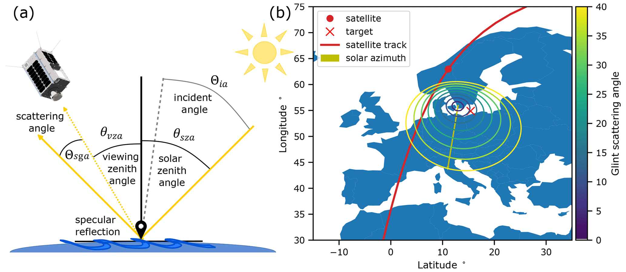
Figure 1 (a) Cross-section of the satellite viewing geometry for offshore sun glint observations. The satellite viewing zenith angle, θ_vza, and solar zenith angle, θ_sza, are measured with respect to the target normal (solid black line). Incoming solar radiation impinges on the water surface at incident angle, Θ_ia, with respect to the wave surface normal (dashed grey line), and undergoes specular reflection towards the satellite. The scattering glint angle, Θ_sga, indicates the angle separating the satellite view from the ideal direct solar specular reflection from a flat, smooth water surface. (b) Example satellite ground track (red line) for viewing an offshore target (red cross) in the Baltic Sea with the sun at 67.6^∘ zenith and 189.4^∘ azimuth (yellow line). The indicated satellite position (red dot) minimizes the scattering glint angle on this pass. Contour lines illustrate the glint scattering angle at intervals of 5^∘ from the satellite's perspective. Viewing the target (red cross) in this example gives a minimum scattering angle of approximately 10^∘.

For a given offshore target, we optimize the amount of light that reaches the detector by finding the satellite position along its track that minimizes the scattering glint angle (Capderou, 2014),

$$\begin{array}{}\text{(2)}& \begin{array}{rl}{\mathrm{\Theta }}_{\mathrm{sga}}& =\arccos \left[\cos \left({\mathit{\theta }}_{\mathrm{sza}}\right)\cos \left({\mathit{\theta }}_{\mathrm{vza}}\right)\right.\\ & \left.-\sin \left({\mathit{\theta }}_{\mathrm{sza}}\right)\sin \left({\mathit{\theta }}_{\mathrm{vza}}\right)\cos \left({\mathit{\varphi }}_{\mathrm{saa}}-{\mathit{\varphi }}_{\mathrm{vaa}}\right)\right],\end{array}\end{array}$$

with respect to the reflecting surface, as illustrated in Fig. 1a. A scattering angle of 0 corresponds to the satellite viewing the center of the glint spot: the direct specular reflection of the sun when the sea surface is flat. As such, the angle will be minimized when the solar and satellite zenith angles are equal, θ_sza=θ_vza, and the azimuths are offset by ${\mathit{\varphi }}_{\mathrm{saa}}-{\mathit{\varphi }}_{\mathrm{vaa}}=\mathrm{180}$^∘. The other angle that affects the signal reaching the detector is the incident angle,

$$\begin{array}{}\text{(3)}& \begin{array}{rl}{\mathrm{\Theta }}_{\mathrm{ia}}& ={\displaystyle \frac{\mathrm{1}}{\mathrm{2}}}\arccos \left[\cos \left({\mathit{\theta }}_{\mathrm{sza}}\right)\cos \left({\mathit{\theta }}_{\mathrm{vza}}\right)\right.\\ & \left.+\sin \left({\mathit{\theta }}_{\mathrm{sza}}\right)\sin \left({\mathit{\theta }}_{\mathrm{vza}}\right)\cos \left({\mathit{\varphi }}_{\mathrm{saa}}-{\mathit{\varphi }}_{\mathrm{vaa}}\right)\right],\end{array}\end{array}$$

which is the angle between the incident light ray and the sea surface normal, as illustrated in Fig. 1a. Higher incident angles increase the surface reflectivity due to Fresnel reflection. Consequently, the signal levels at the detector can change significantly with the solar and satellite viewing geometry, in addition to other environmental conditions such as surface wind speed and sea-surface roughness. We estimate the changes in surface reflectivity using the Cox–Munk sea surface reflection model (Cox and Munk, 1954; Bréon, 1993; Bréon and Henriot, 2006),

$$\begin{array}{}\text{(4)}& \begin{array}{rl}& R\left({\mathit{\theta }}_{\mathrm{sza}},{\mathit{\varphi }}_{\mathrm{saa}},{\mathit{\theta }}_{\mathrm{vza}},{\mathit{\varphi }}_{\mathrm{vaa}},\mathit{\lambda },\mathrm{ws}\right)=\\ & {\displaystyle \frac{\mathit{\pi }{\mathit{\rho }}_{fr}\left({\mathrm{\Theta }}_{\mathrm{ia}},\mathit{\lambda }\right)}{\mathrm{4}\cos \left({\mathit{\theta }}_{\mathrm{sza}}\right)\cos \left({\mathit{\theta }}_{\mathrm{vza}}\right){\cos }^{\mathrm{4}}\left(\mathit{\beta }\right)}}P\left(Z_{\mathrm{up}},Z_{\mathrm{cross}},\mathrm{ws}\right),\end{array}\end{array}$$

which depends on the slopes of the surface waves, Z_up and Z_cross, in the up-wind and cross-wind directions, respectively; the total wave surface slope, $\mathit{\beta }=\arctan \left(\sqrt{Z_{\mathrm{up}}^{\mathrm{2}}+Z_{\mathrm{cross}}^{\mathrm{2}}}\right)$; and the Fresnel reflection coefficient, ρ_fr. $P(Z_{\mathrm{up}},Z_{\mathrm{cross}},\mathrm{ws})$ is the probability distribution function for a wave to have surface slopes Z_up and Z_cross given wind speed, ws, and for which Cox and Munk (1954) suggest using a Gram–Charlier decomposition. We calculate $P(Z_{\mathrm{up}},Z_{\mathrm{cross}},\mathrm{ws})$ using the method in Bréon and Henriot (2006).

While both the scattering angle and the incident angle change the total reflected signal, the scattering angle places the strongest constraints on which satellite passes can be selected to view a nearby target. Large along-track or cross-track angles are sometimes required to minimize the scattering angle in Eq. (2). Since the GHGSat satellites can view targets up to 65^∘ in the along-track direction and up to 55^∘ in the cross-track direction, this enables a larger number of opportunities which can achieve the scattering angle requirements for offshore measurements across a wide range of latitudes and throughout the year.

For each glint observation, the start time of the observation is obtained by propagating the satellite orbit and finding the time that minimizes the scattering angle in Eq. (2). We typically require the minimum scattering angle during an observation to be below 20^∘, as we have found empirically that scattering angles above this value considerably limit the light signal measured by the detector (see Fig. 4a). Figure 1b shows an example satellite ground track for a sun glint measurement of an offshore target with a scattering angle of approximately 10^∘.

Table 1 Observation mode parameters for GHGSat constellation.

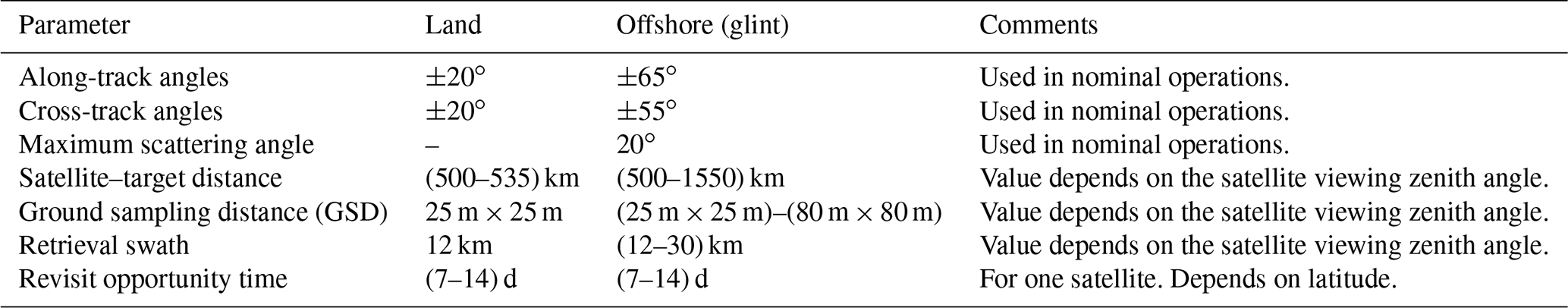
Once the observation begins, the satellites perform a panning manoeuver to acquire several closely spaced images as the target slowly pans through the field of view. Nominal observations consist of 200 frames with a frame period of 100 ms. The camera exposure time is adjusted for each observation based on the predicted reflectivity, obtained using the Cox–Munk sea surface model, and the wind speed and wind direction are obtained from the meteorological database provided by the NASA Goddard Earth Observing System Forward Processing (GEOS-FP) forecast product. Table 1 summarizes the differences in the resulting observation parameters for land and offshore targeted observation modes.

In order to retrieve methane emissions in offshore environments, we use the retrieval algorithm described in Jervis et al. (2021) and which has been validated for targets over land (Sherwin et al., 2023a, b). The algorithm uses a simplified radiative transfer equation in the short-wave infrared where thermal emissions, aerosols, and molecular scattering have been neglected. For each observation, we perform a (1) scene-wide retrieval using the full nonlinear forward model (FM) to determine scene-wide surface and atmospheric state parameters $\widehat{x}$ followed by a (2) per-pixel column density retrieval using a linearized forward model (LFM) evaluated at the linearization point $\widehat{x}$ to determine the surface and atmospheric state parameters at each ground cell.

For each ground cell, we also estimate the methane column density precision by calculating the posterior error on the retrieved methane column density,

$$\begin{array}{}\text{(5)}& \mathrm{\Delta }{X}_{{\mathrm{CH}}_{\mathrm{4}}}\left({\mathrm{mol}\mathrm{m}}^{-\mathrm{2}}\right)={\left({\mathbf{K}}^T{\mathbf{S}}_{\mathrm{o}}^{-\mathrm{1}}\mathbf{K}\right)}^{-\mathrm{1}/\mathrm{2}},\end{array}$$

where S_o is the signal covariance error, which is calculated from the fit residuals during the column retrieval step, and K is the column retrieval Jacobian, which, in Eq. (5), converts the signal error into an error on the retrieved parameters (Ramier et al., 2022). Quality flags are applied when ground cells have a low surface reflectance, below 0.04, or a large posterior methane error, above 0.030 mol m⁻². These values are chosen to balance the number of pixels retrieved against the measurement error. Ground cells that have been flagged are not used in the subsequent source rate quantification.

The output of the column density retrieval produces a map of the state parameters for each ground cell in a reference coordinate frame as measured by the camera. The reference frame coordinate system is then georeferenced onto the appropriate UTM grid by leveraging computer vision reconstruction pipelines (Zhang et al., 2019) and using the satellite position and attitude at the reference frame trigger time. Camera distortion is corrected using pre-flight characterization data.

3 Example plumes

In Fig. 2, we show example retrievals where methane plumes were observed in a variety of offshore locations around the world. In each figure, we show the extracted plume enhancement overlaid on top of the retrieved surface reflectance. The plume mask is generated with a flood-fill algorithm, which uses a threshold to distinguish ground cells in the plume from the background ground cells. Ground cells with a high methane enhancement posterior error are also excluded from the plume mask. In Fig. A1, we show example unmasked methane enhancement fields next to the respective retrieved surface reflectance. The source rates are estimated using the integrated mass enhancement (IME) method as described in Varon et al. (2018). The U₁₀ wind speed is drawn from the GEOS-FP reanalysis product, after which the effective wind speed U_eff is calculated using the method in Maasakkers et al. (2022). The error on the emission rate is obtained from the error on the wind speed, the error on the retrieved methane enhancements, and the error on the IME model, added in quadrature. We use a wind speed error of 2 m s⁻¹, obtained by comparing GEOS-FP with wind measurements at US airports (Varon et al., 2018), which is then propagated through the effective wind speed and source rate calculations.

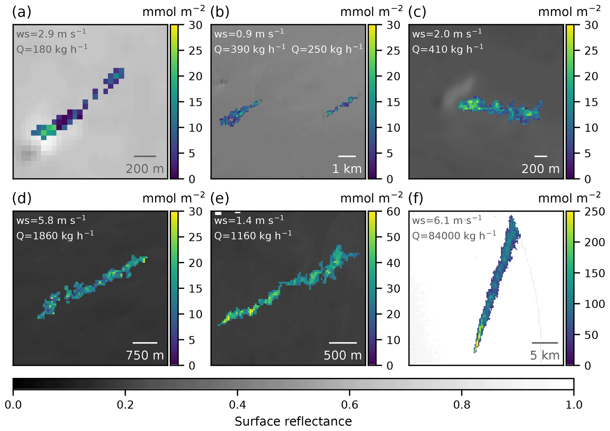
Figure 2 Retrieved offshore methane enhancement fields. The retrieved surface reflectance is plotted with the extracted methane plume overlaid on top. The plume masks show the retrieved methane column density enhancement above the local background in mmol m⁻². Indicated wind speeds are obtained from the GEOS-FP reanalysis product at the observation location and time. (a–d) Examples from offshore shallow water platforms in the Gulf of Mexico for sites off the coast of Louisiana. Plumes measured from (a) a platform on 30 October 2022 with source rate (180 ± 140) kg h⁻¹, (b) two platforms on 5 February with source rate (390 ± 300) and (250 ± 190) kg h⁻¹, (c) a central hub facility on 28 April 2022 with a source rate of (410 ± 230) kg h⁻¹, and (d) a central hub facility on 10 October 2022 with a source rate of (1860 ± 820) kg h⁻¹. (e) Offshore platform off the coast of Africa measured on 24 November 2022 with a source rate of (1160 ± 700) kg h⁻¹. (f) Nord Stream 2 pipeline leak in the Baltic Sea off the coast of Sweden, measured on 30 September 2022 at 10:26 UTC with a source rate of (84 000 ± 24 000) kg h⁻¹.

Between October 2022 and April 2023, we observed a number of plumes at two sites in the Gulf of Mexico in shallow waters off the coast of Louisiana (Fig. 2a–d). Shallow water platforms in the Gulf of Mexico have been found to exhibit super-emitter behaviour above 1000 kg h⁻¹ with high persistence (Ayasse et al., 2022), thereby increasing the carbon intensity of the region (Gorchov Negron et al., 2023). The source rates obtained at these two sites range between 180 and 1860 kg h⁻¹.

In Fig. 2f, we show the methane plume enhancement from the Nord Stream 2 pipeline leak in the Baltic Sea. Following reports of the Nord Stream 2 gas leaks on 26 September 2022, GHGSat immediately began tasking its satellite constellation to detect and quantify methane emissions from the offshore Nord Stream 2 leak in the Baltic Sea. For the Nord Stream incident, while the first attempts by GHGSat and other satellites were unsuccessful due to cloudy conditions, three clear-sky opportunities on 30 September all yielded successful plume detections of the Nord Stream 2 pipeline leak. Figure 2f illustrates the largest of these plumes measured on 30 September 2022 at 10:26 UTC at (84 000 ± 24 000) kg h⁻¹.

For the Nord Stream 2 observation shown in Fig. 2f, the high surface reflectivity near unity reduces the contribution of the retrieved methane enhancement error to the total error, and it is the wind speed error that dominates the total source rate error. On the other hand, for the observations in Fig. 2a–e with lower surface reflectivity, the retrieved methane enhancement error is larger, and its relative contribution to the total source rate error is comparable to the wind speed error. The quantification of errors in the retrieved methane enhancements and their relationship to surface reflectivity are discussed in detail in the next section.

These examples demonstrate the GHGSat constellation's capabilities for monitoring offshore platforms for a wide range of emission rates. With retrieved emission rates ranging from 84 000 kg h⁻¹ down to 180 kg h⁻¹, they represent, respectively, the single largest emission rate ever observed by GHGSat both on- and offshore and the offshore plume with the smallest emission rate detected from space to date.

4 Measurement performance

We empirically estimate the methane column density precision for an ensemble of 80 glint observations of offshore targets taken in 2022 and at multiple locations around the world where no methane plumes were detected. These are taken throughout the year and at multiple locations, as illustrated in the inset of Fig. 3a, to sample a wide variety of environmental and atmospheric conditions. For a uniform background, we expect retrievals of neighbouring pixels to return approximately the same value. Deviations from this can therefore capture the noise in the measurement and the retrieval algorithm. Thus, the methane column density precision of a ground cell can be estimated by looking at the standard deviation of the retrieved methane column density in the surrounding ground cells.

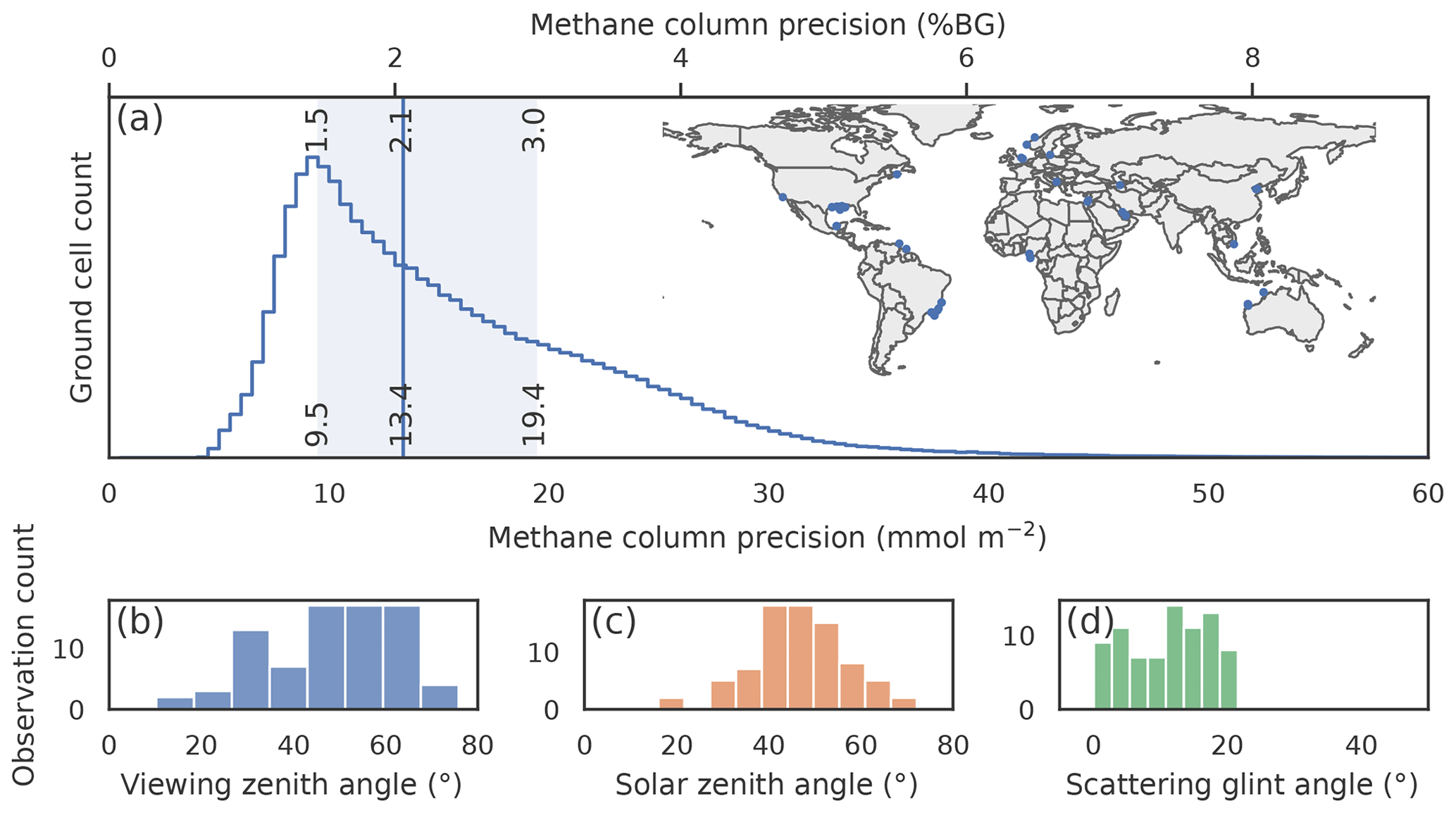
Figure 3 Methane column density precision for offshore glint measurements. (a) Histogram of the standard deviation of the retrieved methane column densities for a moving window with a size of 500 m × 500 m for 80 observations taken in 2022. We find that ground cells between the 25th and 75th percentiles have a standard deviation between 1.5 % and 3.0 % of the methane background column density, with a median value of 2.1 % of background. Inset: target locations for the observations used in the analysis. Histograms of the (b) viewing zenith angle, (c) solar zenith angle, and (d) scattering zenith angle for the observations analyzed. Measurements were performed over a wide range of solar and satellite viewing conditions, with the majority of observations having solar and viewing zenith angles between 20 and 70^∘. Only observations with a glint scattering angle below 20^∘ are used in the analysis (see text for details).

For each observation, we compile a histogram of the standard deviation of a weighted moving filter with a window size of 500 m × 500 m, weighted according to the number of valid non-flagged ground cells in the window. The histogram for a total of 80 observations is shown in Fig. 3a. We find a median column density precision of 2.1 % (13.5 mmol m⁻²) of the background methane column density, with an interquartile range between 1.5 % and 3.0 % (9.6 and 19.6 mmol m⁻²). The median value at 2.1 % is comparable to the observed value on land at 2.0 % (Ramier et al., 2022). On the lower end, we find a cutoff where all 500 m × 500 m ground cells have a column density error above 0.8 % of background. The long tail extending beyond 3.0 % is primarily due to observations with low signal levels, as discussed below.

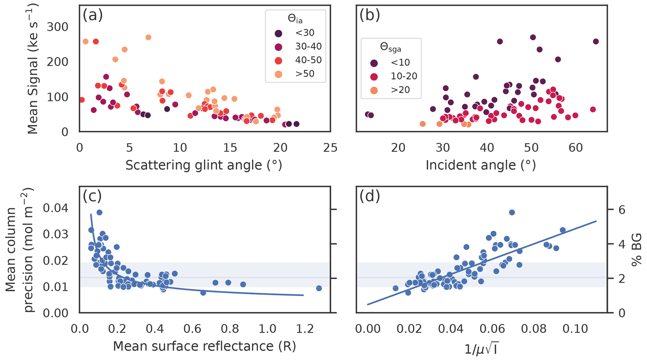
Figure 4 Relationship between mean viewing geometry, signal, and methane column precision for 80 glint observations taken in 2022. (a–b) Effect of the viewing geometry on the mean measured signal. The observation mean signal (ke s⁻¹) decreases with (a) the scattering angle and increases with (b) the incident angle. As the scattering angle increases, the satellite view moves away from the ideal glint spot and the signal decreases, whereas as the incident angle increases, the reflected light at the surface increases due to Fresnel reflection. (c–d) Effect of the change in the signal on the mean column precision for the same observations. The solid line and shaded region indicate the 25th, 50th, and 75th percentiles obtained in Fig. 3. (c) The observation mean column precision is found to be inversely proportional to the mean surface reflectance. The mean column precision decreases rapidly from 4 % at an albedo of 0.1 down to below 2 % at an albedo of 0.3 and continues to decrease steadily beyond this. (d) The mean column precision is found to be linearly proportional to $\mathrm{1}/\mathit{\mu }\sqrt{I}$ from Eq. (6), the inverse of air mass factor times the square root of the mean signal.

For the case of solar illumination, the measured signal, I, is proportional to the surface reflectance, R, and the cosine of the solar zenith angle θ_sza, I∝Rcos (θ_sza). For unpolarized light, the reflectance can be parametrized by two angles, the scattering angle, Θ_sga, and the incident angle, Θ_ia. These two angles will vary with each glint observation depending on the relative positions of the sun, target, and satellite, changing the signal reaching the instrument. The measured mean signal for an ensemble of glint observations is shown as a function of these two angles in Fig. 4a–b. In Fig. 4a, we find the mean signal decreases linearly with the scattering angle. Beyond a glint scattering angle of 20^∘, the mean signal falls below 30 ke s⁻¹, where we find the signal-to-noise ratio on the camera to be too low for the retrieval algorithm to reliably and consistently retrieve methane enhancements. In Fig. 4b, we see that higher incident angles increase the mean signal due to increased Fresnel reflection.

As the signal levels vary with viewing geometry, the column density precision will change. We can estimate how the column density precision scales with signal in the limit where camera random noise dominates the observed measurement error. Starting with Eq. (5), the main contributors to the Jacobian are the column elements involving methane, $\mathbf{K}\approx {\mathbf{K}}_{{\mathrm{CH}}_{\mathrm{4}}}$. The normalized methane Jacobian, ${\mathbf{k}}_{{\mathrm{CH}}_{\mathrm{4}}}={\mathbf{K}}_{{\mathrm{CH}}_{\mathrm{4}}}/I$, can then be shown to be approximately proportional to the air mass factor, ${\mathbf{k}}_{{\mathrm{CH}}_{\mathrm{4}}}\propto \mathit{\mu }\left({\mathit{\theta }}_{\mathrm{sza}},{\mathit{\theta }}_{\mathrm{vza}}\right)\equiv \mathrm{1}/\cos {\mathit{\theta }}_{\mathrm{sza}}+\mathrm{1}/\cos {\mathit{\theta }}_{\mathrm{vza}}$, which accounts for the total path travelled by a light ray. For observations with typical signal levels, the camera random noise can be approximated by the shot noise, which is modelled by a Poisson distribution, and, as a result, the signal covariance, S_o, is proportional to the measured signal, ${\mathbf{S}}_{\mathrm{o}}\propto {\mathit{\sigma }}_N^{\mathrm{2}}\propto I$. Using these approximations, we can relate the column precision in Eq. (5) to the total signal reaching the detector,

$$\begin{array}{}\text{(6)}& \begin{array}{rl}& \mathrm{\Delta }{X}_{{\mathrm{CH}}_{\mathrm{4}}}\left({\mathrm{mol}\mathrm{m}}^{-\mathrm{2}}\right)\approx {\left(I{\mathbf{k}}_{{\mathrm{CH}}_{\mathrm{4}}}^T{\mathit{\sigma }}_N^{-\mathrm{2}}I{\mathbf{k}}_{{\mathrm{CH}}_{\mathrm{4}}}\right)}^{-\mathrm{1}/\mathrm{2}}\\ & \propto {\displaystyle \frac{\mathit{\alpha }{\mathit{\sigma }}_N}{\mathit{\mu }I}}\propto {\displaystyle \frac{\mathit{\alpha }}{\mathit{\mu }\sqrt{I}}}\\ & \propto {\displaystyle \frac{\mathit{\alpha }}{\mathit{\mu }\sqrt{R\left({\mathit{\theta }}_{\mathrm{sza}},{\mathit{\theta }}_{\mathrm{vza}},{\mathit{\varphi }}_{\mathrm{saa}},{\mathit{\varphi }}_{\mathrm{vaa}},\mathit{\lambda },\mathrm{ws}\right)\cos \left({\mathit{\theta }}_{\mathrm{sza}}\right)}}},\end{array}\end{array}$$

where α is a proportionality constant to be determined empirically. We test and empirically verify this derived scaling relationship in Fig. 4c–d.

Using the 80 observations in Fig. 3, we break down the estimated column precision by showing how it varies with different retrieved parameters. In Fig. 4c–d, we plot the mean column precision of each observation as a function of the retrieved mean surface reflectivity (Fig. 4c) and the scaling factor $\mathrm{1}/\mathit{\mu }\sqrt{I}$ from Eq. (6) (Fig. 4d). In Fig. 4c, we find the mean column precision is inversely proportional to the surface reflectivity; a higher surface reflectivity leads to a higher light signal at the detector, and this translates into a reduction in random errors. In Fig. 4d, we find the mean column precision to be linearly proportional to the scaling factor, $\mathrm{1}/\mathit{\mu }\sqrt{I}$, with slope α=0.288 mol m⁻² (ke s⁻¹)⁻¹ and intercept 0.003 mol m⁻². The observed variations in the methane column precision can therefore be captured by the change in air mass factor and signal levels in Eq. (6) over the large range of solar and viewing angles under study.

5 Detection limit for offshore measurements

The detection limit defines an instrument's ability to detect plumes. For observations on land, the detection limit of GHGSat's satellite remote sensing instruments has been assessed with controlled-release experiments, either through internally organized campaigns within GHGSat or single-blind campaigns organized with third parties (Sherwin et al., 2023b; Darynova et al., 2023). However, such experiments are extremely challenging in offshore environments for both operational and regulatory reasons, and, as such, we assess the glint instrument detection limit through a combination of the empirical measurement results presented in the previous section and analytical modelling.

In the limit of a single pixel detection, the methane detection limit of an instrument is driven by the following equation (Jacob et al., 2016):

$$\begin{array}{}\text{(7)}& Q_{\lim }=M_{{\mathrm{CH}}_{\mathrm{4}}}UGq\mathrm{\Delta }{X}_{{\mathrm{CH}}_{\mathrm{4}}},\end{array}$$

where $M_{{\mathrm{CH}}_{\mathrm{4}}}$ is the molar mass of methane, U is the wind speed, G is the ground sampling distance (GSD), $\mathrm{\Delta }{X}_{{\mathrm{CH}}_{\mathrm{4}}}$ is the methane column precision, and q determines the number of standard deviations above the noise required to reliably assign a methane enhancement to a pixel. Values of q=2 and q=5 have been proposed for detection and quantification, respectively (Jacob et al., 2016). We follow this convention and assume that methane plume enhancements must be at least 2 times above the noise floor to enable plume detection. Equation (7) implies the detection limit, Q_lim, increases proportionally with the wind speed, the GSD, and the column precision. GHGSat's instruments operating in targeted mode over land have a ground sample distance of 25 m and a median methane column density noise of 0.013 mol m⁻², or 2 % of the background column density. Assuming a wind speed of 3 m s⁻¹ and a value of q=2 for detection, Eq. (7) gives a detection limit of 120 kg h⁻¹, a value commensurate with results obtained from controlled-release experiments on the ground (McKeever and Jervis, 2021; Ramier et al., 2022).

For land observations operated in nadir mode over diffuse surfaces, the GSD and column precision vary little with viewing angle, and, as a result, the detection limit remains fairly constant across different observations. With glint observations, however, both the ground sample distance and the column density noise can vary significantly for different viewing geometries, and these affect the detection limit of an observation. In order to estimate the detection limit with glint observations, we approximate the GSD,

$$\begin{array}{}\text{(8)}& G={\displaystyle \frac{h_{\mathrm{sat}}{p}_{\mathrm{pix}}}{f}}{\displaystyle \frac{\mathrm{1}}{\cos {\left({\mathit{\theta }}_{\mathrm{vza}}\right)}^{\mathrm{1}/\mathrm{2}}}},\end{array}$$

as the ratio of the satellite target distance, h_sat; the pixel pitch, p_pix; and the instrument focal length, f. The satellite target distances can be expressed in terms of the satellite's nadir altitude, h₀; its viewing zenith angle; and the Earth's radius, R_E, $h_{\mathrm{sat}}=\sqrt{R_{\mathrm{E}}^{\mathrm{2}}{\cos }^{\mathrm{2}}\left({\mathit{\theta }}_{\mathrm{vza}}\right)+h_{\mathrm{0}}(h_{\mathrm{0}}+\mathrm{2}{R}_{\mathrm{E}})}-R_{\mathrm{E}}\cos {\mathit{\theta }}_{\mathrm{vza}}$. The inverse cosine with exponent $\mathrm{1}/\mathrm{2}$ is obtained from the geometric mean of the GSD along the two camera axes, one which increases only with the satellite-target distance, h_sat, and the other which increases due to both the satellite target distance and pixel projection effects, $h_{\mathrm{sat}}/\cos \left({\mathit{\theta }}_{\mathrm{vza}}\right)$. Furthermore, Eqs. (7) and (8) can provide an initial estimate of the expected range for the glint detection limit. Fixing the methane column density precision, $\mathrm{\Delta }{X}_{{\mathrm{CH}}_{\mathrm{4}}}$, at the measured median value in Fig. 3a, viewing zenith angles between 20 and 70^∘ from Fig. 3b, and assuming winds speeds of 3 m s⁻¹, we find a detection limit of approximately 135 kg h⁻¹ at 20^∘ and 500 kg h⁻¹ at 70^∘.

To take into account the variations in the methane column density precision, we substitute Eqs. (6) and (8) into Eq. (7). We find a detection limit that scales as

$$\begin{array}{}\text{(9)}& Q_{\lim }\approx \mathit{\alpha }{M}_{{\mathrm{CH}}_{\mathrm{4}}}U{\displaystyle \frac{p_{\mathrm{pix}}{h}_{\mathrm{sat}}}{f\cos {\left({\mathit{\theta }}_{\mathrm{vza}}\right)}^{\mathrm{1}/\mathrm{2}}}}{\displaystyle \frac{q}{\mathit{\mu }\sqrt{I}}}.\end{array}$$

Equation (9) connects the detection limit of an observation to the measured signal level and the viewing geometry. The detection limit increases in proportion to the satellite target distance, h_sat, and in inverse proportion to the square root of the measured signal, I∝Rcos (θ_sza), and the surface reflectivity, R. By simulating how the signal varies for different viewing geometries, target latitudes, and times of year, we can estimate the glint detection limit of the GHGSat constellation.

6 Detection limit from orbital simulations

To estimate the detection limit, we propagate a series of sun-synchronous satellite orbits at an altitude of 535 km and with a local time at the descending node (LTDN) between 10:00 and 14:00 LTDN in 1 h steps for a period of 60 d around the summer and winter solstices and the spring and fall equinoxes: March, June, September, and December 2022. We simulate observations of glint targets at latitudes between −60 and 60^∘ and at these four different times of year. For each target observation, we select the observation start time by minimizing the scattering angle in Eq. (2). Satellite passes are deemed valid when the minimum scattering angle is below 20^∘ and the satellite viewing zenith angle is below 80^∘. In this way, the total number of observations of each target varies between 30 and 180 depending on the latitude.

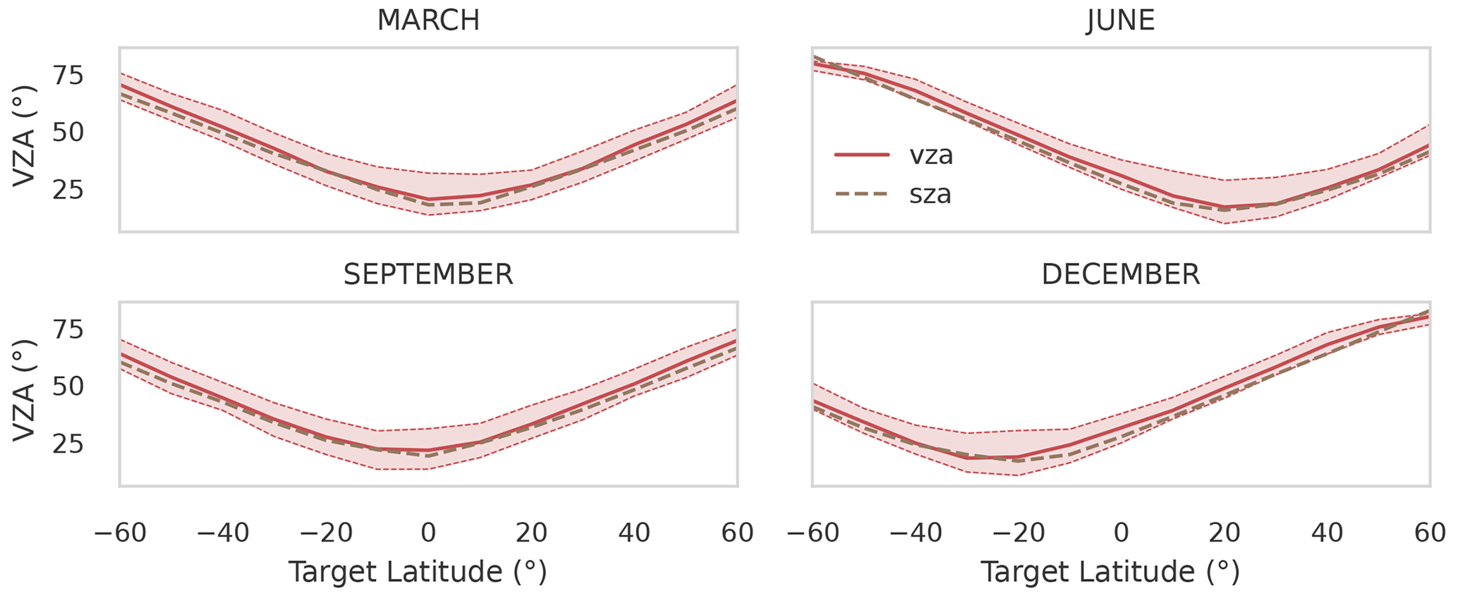
Figure 5 Satellite viewing zenith angle and solar zenith angle for the ensemble of simulated satellite observations at different latitudes and seasons. Dashed and solid red lines show the 25th, 50th, and 75th viewing zenith angle percentiles for the ensemble of observations at each latitude. The dashed black line illustrates the median solar zenith angle for each latitude. For each satellite pass, the observation center is obtained by minimizing the scattering angle, Θ_sga. We find that the optimal viewing zenith angle for the ensemble of observations tracks the solar zenith angle as a function of latitude and season. At high latitudes, when the sun is closer to the horizon (large SZA), the satellite is constrained to stay close to the horizon (large VZA) to minimize the glint scattering angle.

For each valid observation, we tabulate the solar and satellite zenith and azimuth angles at the observation center. The distribution of viewing zenith angles for each latitude and season is illustrated in Fig. 5. During the equinoxes (March/September), the viewing zenith angle across all simulated observations is small near the Equator, whereas during the solstice (June/December), the viewing zenith angle is small near the tropics at ±23.5^∘. At higher latitudes, the viewing zenith angle increases when the solar zenith angle is correspondingly large. We thus find that for glint observations to minimize the scattering angle, the satellite viewing zenith angle will, on average, track the solar zenith angle throughout the year.

The solar and satellite angles are then used to calculate the predicted signal, I, and, second, used to determine the methane column precision, $\mathrm{\Delta }{X}_{{\mathrm{CH}}_{\mathrm{4}}}$. The predicted signal is calculated from an empirically measured instrument transmission function and the surface reflectance using the Cox–Munk model (Bréon and Henriot, 2006), assuming a fixed wind speed of 3 m s⁻¹ and averaged over four wind directions, 0, 90, 180, and 270^∘ from the north. Once the signal is calculated, we estimate the column precision from the signal–noise relationship following Eq. (6) and the empirically measured proportionality constant obtained in Fig. 4d.

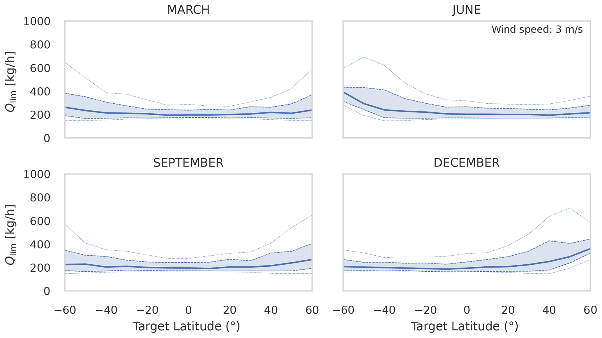
Figure 6 Estimated detection threshold as a function of latitude for spring/fall equinoxes and summer/winter solstices. For each period and target latitude, we simulate 60 d of satellite observations for sun-synchronous orbits at 535 km with LTDN between 10 and 14 h. Observations with a scattering glint angle below 20^∘ are retained. The column density noise and GSD are calculated from the predicted signal based on the solar and satellite viewing angles. Dashed and solid lines show the 5th, 25th, 50th, 75th, and 95th detection threshold percentiles for the ensemble of observations at each latitude. Filled values show the range between the 25th and 75th percentiles. We find that the detection threshold is lower at latitudes and times of the year when the sun is higher in the sky: near equatorial latitudes in the summer and near the tropics in the spring and fall.

Table 2 Detection limit range estimated from simulated glint (offshore) measurements for two latitude bands. Values represent quantiles in kg h⁻¹ averaged over each specified latitude band and season in Fig. 6 rounded to the nearest 10.

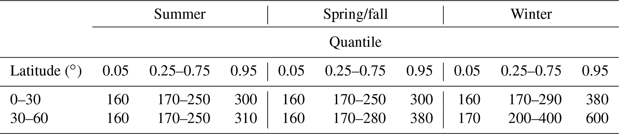
The detection limit is then calculated using Eq. (7), using a value of q=2, and the results are presented in Fig. 6. Solid and dashed lines show the detection threshold percentiles for the ensemble of observations at each target. We find the detection threshold varies with latitude and season. During the summer solstice, the range of detection thresholds is lowest in the tropics near ±23.5^∘, whereas during the equinoxes in March and September, the range of detection thresholds is lowest near the Equator. We find an increase in the detection limit at higher latitudes for all seasons. The increase is larger in the winter solstice, which corresponds to northern latitudes in December and to southern latitudes in June. We summarize these findings in Table 2, which shows the mean detection limit range for two latitude bands and the four seasons. The values in the table for the 5th and 95th percentiles vary between 160 and 600 kg h⁻¹.

The variations in the detection limit in Fig. 6 can be understood by comparing them to the variations in the viewing zenith angle in Fig. 5. The viewing zenith angle affects both the GSD and the methane column precision, which in turn affects the detection limit. Observations with larger viewing zenith angles will have a larger satellite target distance and consequently a larger GSD, which will increase the detection limit. Larger viewing angles will, however, decrease the methane column density noise due to an increase in both the signal level reaching the instrument through larger Fresnel reflection and the air mass factor, μ. While the decrease in the methane column density noise will decrease the detection limit, this effect is small compared to the effect of the GSD. As such, the changes in the detection limit in Fig. 6 are approximately correlated with the changes in the viewing zenith angle in Fig. 5. These results illustrate the main difference between glint observations and targeted land observations, namely, that the viewing conditions for each glint observation play an important role in determining the detection limit, and these vary with latitude and season.

7 Conclusions

We have demonstrated the capability for satellite-based remote sensing to detect and monitor both large and small offshore methane emissions in near-real time with the GHGSat constellation. Detection and quantification of offshore methane emissions are operational now and have been demonstrated with multiple examples, including the smallest offshore emissions measured from space to date.

Glint observations are unique in that the viewing conditions can change with every observation, and this affects the signal levels, the methane column density precision, and the ground sample distance (GSD). We empirically estimate a median column precision of 2.1 % of the background methane column density, a value comparable to what we obtain on land. Furthermore, by combining an analytical model of the detection threshold with empirical measurements of the column precision, we find a detection limit that can vary between (160–600) kg h⁻¹ depending on the target latitude and time of year of the observation. The detection limit is predicted to be better at lower latitudes and in summer months when the solar zenith angle is small. We note that while the detection limit values are specific to the GHGSat constellation, the formulas and scaling relationships obtained are general and would apply to any satellite measurement of atmospheric gases in a glint configuration.

The analysis presented applies to an ensemble of simulated orbits for a few specific targets. In practice, with point source imagers, a satellite operator must choose to observe select targets from a large ensemble on any given day. It should therefore be possible to optimize the selection of targets and the selection of the satellite pass to view those targets based on criteria that include minimizing the detection limit. Moreover, the analytical calculation of the detection limit assumes single pixel detection. However, with point source imagers, multiple pixels are typically required to confirm a detection. While this may change the detection limit for a given latitude and season, we do not expect this to affect the scaling relationships. Further work would be required to understand the impact of requiring multi-pixel detection when estimating a detection limit. Ultimately, controlled-release experiments are desirable to validate the glint detection limit. However, due to operational and regulatory complexities of offshore controlled-release experiments, simultaneous satellite measurements with aircraft or other ground-based instruments across many locations may be a good alternative.

With three additional satellites planned for launch by the end of 2023, the GHGSat satellite constellation will have 10 operational satellites in orbit for detecting and quantifying methane emissions. With an increasing number of satellites and as more data are collected, the detection limit model can be refined and, eventually, validated through controlled releases or cross-validated with other instruments. The methods and analysis presented here will also be applicable to the upcoming CO₂ satellite to be launched at the end of 2023. As the constellation continues to grow, this will enable the detection; quantification; and, ultimately, the mitigation of methane emissions from any site, on- and offshore, with near-daily revisit opportunity times.

Appendix A: Additional figure

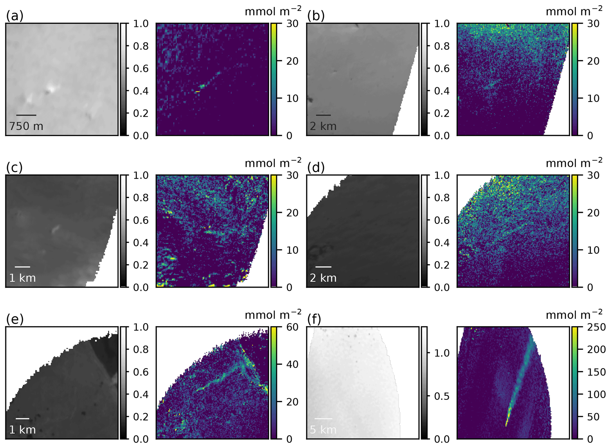
Figure A1 Retrieved offshore methane enhancement and surface reflectance fields for the plumes in Fig. 2. In the left plot, the retrieved surface reflectance is plotted in a region of interest centered on the plume. In the right plot, the retrieved methane enhancement above the local background is shown in units of mmol m⁻² for the corresponding region of interest.