Design and evaluation of BOOGIE: a collector for the analysis of cloud composition and processes

In situ cloud studies are fundamental to study the variability in cloud chemical and biological composition as a function of environmental conditions and assess their potential for transforming chemical compounds. To achieve this objective, cloud water collectors have been developed in recent decades to recover water from clouds and fogs using different designs and collection methods. In this study, a new active ground-based cloud collector was developed and tested for sampling cloud water to assess the cloud microbiology and chemistry. This new instrument, BOOGIE, is a mobile sampler for cloud water collection that is easy to operate with the objective of being cleanable and sterilisable, respecting chemical and microbial cloud integrity, and presenting an efficient collection rate of cloud water. Computational fluid dynamics simulations were performed to theoretically assess the capture of cloud droplets by this new sampler. A 50 % collection efficiency cutoff of 12 µm has been estimated. The collector was deployed at Puy de Dôme station under cloudy conditions for evaluation. The water collection rates were measured at 100 ± 53 mL h⁻¹ for a collection of 21 cloud events; considering the measured liquid water content, the sampling efficiency of this new collector has been estimated at 69.7 ± 11 % over the same set of cloud events. BOOGIE was compared with other active cloud collectors commonly used by the scientific community (Cloud Water Sampler and Caltech Active Strand Cloud Collector version 2). The three samplers presented similar collection efficiencies (between 53 % and 70 % on average). The sampling process can affect the endogenous cloud water microflora, but the ATP $/$ ADP (adenosine triphosphate and adenosine diphosphate) ratios obtained from the samplers indicates that they are not stressful for the cloud microorganisms. The chemical compositions of hydrogen peroxide, formaldehyde, and major ions are similar between the collectors; significant variability is observed for magnesium and potassium, which are the less concentrated ions. The differences between collectors are the consequence of different designs and the intrinsic homogeneity in the chemical composition within the cloud system.

1 Introduction

The chemical composition of clouds is highly complex because it results from various processes: (1) the mass transfer of soluble compounds from the gas phase into cloud droplets, (2) dissolution of the cloud condensation nuclei released into the aqueous phase as a complex mixture of soluble molecules, and (3) photochemical and biological transformations leading to new chemical products (Herrmann et al., 2015).

Field experiments to characterise this multiphasic medium were developed in the 1950s but increased in the 1980s because of precipitation acidification through sulfur oxidation in cloud droplets (Munger et al., 1983; Hoffmann, 1986; Kagawa et al., 2021). These studies have highlighted that cloud and fog processing is efficient and plays a major role in air pollution by transforming gases and aerosol particles. Numerous investigations have focused on inorganic compounds that control aqueous-phase acidity (Pye et al., 2020). The production of strong acids has been assessed because it increases particle mass when clouds or fog evaporate and leads to acidic deposition when clouds precipitate (Tilgner et al., 2021). Early in the 1990s and much more so in the 2000s, researchers investigated the composition of dissolved organic matter in cloud or fog water, which has multiple natural and anthropogenic sources of primary or secondary origin (Herckes et al., 2013). Based on scientific issues, specific classes of compounds have been targeted, such as short-chain carboxylic acids and carbonyls (Löflund et al., 2002; Munger et al., 1995; Sun et al., 2016) and more recently carbohydrates and amino acids (Triesch et al., 2021; Renard et al., 2022). Attention has also been paid to the detection of pollutants with strong sanitary effects, such as polycyclic aromatic hydrocarbon (PAH), phenols, and phthalates (Lüttke et al., 1999; Li et al., 2010; Lebedev et al., 2018; Ehrenhauser et al., 2012), because they can impact ecosystems through precipitation (Wright et al., 2018). Recent investigations using high-resolution mass spectrometry have revealed the complexity of the organic matrix, with thousands of detected molecules (Zhao et al., 2013; Cook et al., 2017; Bianco et al., 2018; Sun et al., 2021). This organic matter is processed during the cloud lifetime and has raised new scientific questions such as the formation of secondary organic aerosol by aqueous-phase reactivity (aqSOA) (Blando and Turpin, 2000; Lamkaddam et al., 2021) and light-absorbing material referring to brown carbon (BrC) (Laskin et al., 2015). Microorganisms are also present and active in cloud droplets (Amato et al., 2005; Vaïtilingom et al., 2012; Xu et al., 2017; Hu et al., 2018). They can be incorporated because they serve as cloud condensation nuclei (Bauer et al., 2002; Deguillaume et al., 2008) and can impact cloud water composition through their metabolism by consuming or producing new molecules (Liu et al., 2023; Vaïtilingom et al., 2013; Pailler et al., 2023). Many investigations have focused on biological cloud characterisation (Amato et al., 2017; Wei et al., 2017).

Monitoring cloud chemical and biological compositions is crucial for evaluating the role of key environmental parameters such as emission sources, atmospheric transport and transformations, and physicochemical cloud properties such as cloud acidity or microphysical cloud properties (liquid water content – LWC – and size distribution of cloud droplets). Specific sites or aircraft campaigns allow the collection of cloud water influenced by marine (MacDonald et al., 2018; Gioda et al., 2011), continental (van Pinxteren et al., 2016; Hutchings et al., 2009; Lawrence et al., 2023; van Pinxteren et al., 2014), and urban emissions (Li et al., 2020; Guo et al., 2012; Herckes et al., 2002) over various continents (mainly Europe, North America, Asia). Owing to their poor accessibility and remoteness, certain geographical locations have been less investigated, such as the Arctic region (Adachi et al., 2022), tropical environments (Dominutti et al., 2022), or marine surfaces (van Pinxteren et al., 2020). Field experiments combining cloud water and gaseous-phase chemical characterisation have also been conducted to evaluate the partitioning of molecules between these two phases and whether bulk cloud water obeys Henry's law (van Pinxteren et al., 2005; Wang et al., 2020). Bulk aqueous cloud media are used for laboratory investigations to study the aqueous transformations induced by light and the presence of microorganisms (Schurman et al., 2018; Bianco et al., 2019).

Therefore, the scientific community requires regular and long-term measurements of cloud chemical and biological parameters. However, cloud-sampling procedures are challenging. In recent decades, different samplers have been developed and deployed in the field, which can be operated under specific environmental conditions and present different collection efficiencies possibly impacted by meteorological conditions. These are commonly based on the impact of cloud droplets on the collector surface and avoid the collection of small droplets (< 5 µm in diameter). Their collection efficiency and 50 % collection cutoff diameter (d50) were calculated and estimated to evaluate the accuracy of droplet collection by the sampler. Monitoring of the microphysical cloud properties (LWC and size distribution) is required to assess this. These samplers refer to “bulk” cloud water collectors because they group droplets of different sizes. Many types of collectors can be listed: active or passive ground- or aircraft-based and single- or multi-stage. Passive collectors are dependent on wind speed because the air needs to flow through them, allowing sampling. Active collectors are ground-based collectors through which air-containing droplets are forced to flow inside the system by devices such as pumps or ventilator fans. They have been designed and commonly used to obtain higher volumes of water required for laboratory investigations. Ground-based samplers are easy to install, inexpensive, and suitable for long-term observations. Samplers installed on aircraft are less widely used, and recent developments by Crosbie et al. (2018) presenting a new axial cyclone cloud water collector have been shown to strongly improve the collection efficiency of cloud droplets compared to previous samplers. All these samplers are described in reviews where their designs, advantages, limitations are presented (Roman et al., 2013; Skarżyńska et al., 2006).

Two types of ground-based active samplers are often used by the scientific community to monitor cloud chemistry and microbiology: the Cloud Water Sampler (CWS) from Vienna University (Kruisz et al., 1993) and the Caltech Active Strand Cloudwater Collector (CASCC) from the California Institute of Technology (Daube et al., 1987; Demoz et al., 1996; Collett et al., 1990). These collectors have been adapted for long-term monitoring (Gioda et al., 2013; Guo et al., 2012; Deguillaume et al., 2014; Renard et al., 2020) and specific field campaigns (Wieprecht et al., 2005; van Pinxteren et al., 2016; Li et al., 2017, 2020; Bauer et al., 2002).

The Puy de Dôme (PUY) station is a reference site for the collection of cloud water from samples collected between 2001 and the present. Historically, the CWS has been widely used for microbial and chemical atmospheric studies at this site (Marinoni et al., 2004, 2011; Bianco et al., 2017; Joly et al., 2014). This model can collect wet or supercooled droplets, even at high wind speeds. It is made of aluminium or Teflon; the collection vessel can be removed for sterilisation and cleaning. However, the collected water volume of 10–60 mL h⁻¹ is a limit for chemical and microbial analyses that require increasing volumes. For long collection times, the vessel should be removed regularly to transfer the water into a sterile storage bottle. These manipulations expose the samples to contamination. The aspiration system must be powerful and, consequently, heavy and energy-consuming, which limits mobile sampling. The objective of this study was to present a ground-based cloud collector that responds to different constraints. This tool should be suitable for analysing cloud microbiology and chemistry, be easy to clean and sterilise, allow the collection of high volumes of water, and be easy to deploy for field campaigns (light and low energy consumption). To achieve these objectives, we developed a collector named BOOGIE. This study describes this instrument and compares it to other commonly used samplers to evaluate its efficiency.

2 Materials and methods

2.1 Conception of the BOOGIE cloud collector

The 3D drawing was performed with Autodesk^® Inventor 2016 and recently updated using the 2019 version. The prototype of the collector used in this study was fabricated on an aluminium stand (Al 5754 and 6060). This material exhibits robust properties and can be easily sterilised by autoclaving before field collection. Aluminium plates were cut using a laser and folded using a metal press. The collection funnel was adapted to a GL 45 thread to directly screw borosilicate glass or polytetrafluoroethylene (PTFE) bottles. All the aluminium parts were treated by QUANALOD^® anodisation, with thickness of 20 µm, suitable for aluminium objects exposed to harsh environmental conditions. All parts were thoroughly cleaned to eliminate all manufacturing residue, and several cycles of sterilisation by autoclaving (121°, 20 min per cycle) were performed to clean the collector.

The vacuum inside the collector was ensured by an axial fan (EMB-papst©, model 6300TD, S-Force, 40 W, 12 V DC) able to work under wet conditions and temperatures of −20 to 70 °C. It has a fan diameter of 172 mm and a theoretical maximum flow capacity of 600 m³ h⁻¹ (manufacturer data). It is equipped with a controlled voltage for speed setting, which allows modulation of the fan velocity according to 10 increasing intensities. To measure the air inlet and outlet velocity, a thermal anemometer efficient from 0.2 to 20 m s⁻¹ was used (model Lutron AM-4204 from RS PRO©).

2.2 Computational fluid dynamics (CFD) simulations

Finite-element modelling and simulations were performed using Simcenter 3D software from Siemens Industry Software Inc., version 2022.1. The solver environment was Simcenter 3D Thermal/Flow Advanced Flow. The flow and particle tracking solvers are proprietary to Maya Heat Transfer Technologies. Other numerical computations and figures were performed using MATLAB version 2021a.

The fluid domain is represented by the inner volume of the collector. To compute a realistic flow inside the collector, it is necessary to consider the structure of the collector, which is composed of thin walls and metal plates, to enable air deflection and the collection of cloud water droplets. The Simcenter 3D software allows the generation of a volume or mesh directly from the boundaries of different parts of the collector; however, this method was unsuitable because of the thin inner walls. The fluid domain was built using successive Boolean subtractions by leaving a void in the right place, leading to a realistic geometry of the air volume (Fig. S1a in the Supplement).

A finite-element mesh was created using CTETRA4 solid elements. The element size was variable: the internal mesh size was set to 20 mm, whereas the element size was set to 24 mm on the rear faces next to the fan and to only 4 mm on the front face, allowing air deflection and the collection of droplets (Fig. S1b). The total numbers of elements and nodes were 869 799 and 178 610, respectively.

For the air inlet flow, three slots of the collector front face were defined as the inlet flow boundary conditions. The flow direction was perpendicular to the front face and the external absolute pressure was equal to the ambient pressure. For the air outlet flow, air velocity was applied to the rear circular face representing the fan. The magnitude varied according to the velocity ranges. The vector was perpendicular to the face.

The fluid is the standard air at the altitude of 1500 m (i.e. summit of the PUY) at 15 °C, with the following physical characteristics: 1.1 kg m⁻³ for the mass density and 1.75 kg m⁻¹ s⁻¹ for the dynamic viscosity.

The outlet velocity of the fan can be modulated among 10 intensities. The resulting air inlet volume flows have been measured using a hot-wire anemometer located in front of the slots. The surface area of the fan outlet was 17 671 mm², and the total area of the three inlet slots was 10 900 mm². Therefore, there was a theoretical ratio of 1.6 between the air inlet volume flow and the air outlet volume flows. To agree with the measured air inlet volume flow, the outlet velocities for the collector simulations were varied for the CFD simulations between 1 and 10 m s⁻¹ in 1 m s⁻¹ steps.

Different particles were used in the simulation. The water drops were injected into the flow at the three air inlet slots. Eight different values of drop diameter were selected between 5 and 20 µm. The water droplets were considered spherical. The drag coefficient was automatically calculated using the Reynolds number. The density of water was assumed to be 1 kg dm⁻³. Gravity was applied to the cloud particles, and the gravity vector was defined as the −Z axis with an acceleration amplitude of 9.81 m s⁻². The sizes and masses of each particle class are summarised in Table S1 in the Supplement.

In the airflow inside the collector, three vertical plates participated in droplet collection. If cloud water drops impact them, they should flow to the bottom of the funnel. Therefore, there is a specific surface configuration; if the water drops stick to the collection face, they do not rebound.

We selected the fully coupled pressure–velocity solver to solve the mass and momentum equations simultaneously for each time step. The solver iterates the pressure and velocity solutions until convergence is achieved at each time step. Modelling fluid flow turbulence is crucial for accurately simulating airflow. The flow solver uses different turbulence models that add a viscosity term to the Navier–Stokes governing equations. The two-equation model computes the viscosity term using two additional equations that are solved in parallel with the Navier–Stokes equations. Among the two-equation models, the k–ω turbulence model was selected for this study. The steady-state time step was fixed to 0.01 s for all the model simulations.

For the steady-state simulation, the flow was fully developed, and its properties (velocity, pressure, and turbulence) were used in the particle-tracking equation. During the analysis, the software solved the equation of motion for each particle once per time step. Notably, because the particle-tracking simulation is independent of the flow simulation, the particles do not affect the 3D flow. The injection duration in the fluid domain was 60 s, which is a good compromise between the relevant calculation and a reasonable simulation time.

2.3 Experiments: intercomparison of samplers

2.3.1 Sampling site

The testing site of the different cloud collectors was the observatory of the PUY summit at 1465 m above sea level. It is part of the Cézeaux-Aulnat-Opme–Puy De Dôme (CO-PDD) instrument platform for atmospheric research (Baray et al., 2020). PUY is recognised as a global station in the Global Atmosphere Watch (GAW) network and is part of European and national research infrastructure including the Aerosol Cloud and Trace Gases Research Infrastructure (ACTRIS) and the Integrated Carbon Observing System (ICOS). PUY is often located in the free troposphere, particularly during cloud events, and the characterised air is representative of synoptic-scale atmospheric composition. Various biological, physical, chemical, and cloud microphysical parameters were monitored on site. For cloud microphysical properties, we use the ground-based scattering laser spectrophotometer PVM-100 for cloud droplet volume measurements from Gerber Scientific, Inc. (Reston, VA, USA). This instrument measures the laser light scattered in the forward direction by the cloud droplets. It allows evaluating the particle volume density (or LWC: liquid water content) and the particle surface area density (PSA). The effective radius R_eff can be calculated using LWC and PSA; it is an estimate of the average size of the cloud droplet population and does not represent the mean physical radius (Guyot et al., 2015). All cloud microbiology and chemistry data are available in the PUYCLOUD database (https://www.opgc.fr/data-center/public/data/puycloud, last access: 15 February 2025).

2.3.2 Cloud collectors

Two bulk cloud collectors were compared with a newly developed BOOGIE collector. These are active ground-based collectors commonly used in cloud field studies. They have different collection efficiencies, resulting in different volumes of cloud water that can be sampled. Cloud water collectors are generally designed to avoid the particles below 5 µm to avoid sampling the interstitial aerosol around the droplets. This is a compromise to obtain a sufficient volume of water with less contamination from dry and deliquescent particles. Typically, the smallest droplets were not sampled. The 50 % collection efficiency cutoff, based on the droplet diameter, is often predicted from the impaction theory and strongly depends on the aerodynamic design of the impactor and the airflow rate (Berner, 1988; Schell et al., 1992). The collection efficiency for in situ conditions will depend on the LWC, and the meteorological conditions could strongly perturb the way the collectors are able to impact cloud droplets.

Caltech Active Strand Cloud water Collector: CASCC2

A compact version of the original CASCC collector was used and lent by the Institut de Radioprotection et de Sûreté Nucléaire (IRSN). This sampler, named CASCC2, was constructed according to the recommendations of Demoz et al. (1996). It has an estimated cutoff diameter of 3.5 µm (droplet diameter collected with 50 % collection efficiency). This collector has a metal body, stainless-steel collection strands, and a metal collection trough. The airflow passed through a set of six rows of stainless-steel strings (diameter, 0.5 mm) with a velocity of 8.6 m s⁻¹. The strings were vertically tilted 35°. The collector design has been shown to generate a stable airflow inside of 348 m³ h⁻¹. Demoz et al. (1996) proposed a correction to estimate the fraction of air that actually induces the sampling of the droplets; this was calculated to be 86 %, resulting in a 299 m³ h⁻¹ airflow. The volume fraction of the ambient droplet distribution collected was evaluated in Demoz et al. (1996), who showed that this fraction is close to 1 over most of the LWC range (higher than 95 % > 0.1 g m⁻³ of LWC). Therefore, at the end, a resulting sampled airflow at 284 m³ h⁻¹ (4.73 m³ min⁻¹) could be estimated. Cloud droplets coalesce on the strands and fall into a bottle through a Teflon tube owing to the combination of gravity and aerodynamic drag. A description of the sampler is provided in Fig. S2.

The collector body was stainless steel, the inlet contained the impaction rows, and the sample drainage was removed before each sampling for cleaning and sterilisation. A sterilised amber glass bottle was placed under the sample drainage during collection. The CASCC2 was also not operated with a downward-facing inlet, allowing the exclusion of the collection of rain. This cloud collector was not adapted for temperatures < 0 °C because droplets freeze upon impaction on metallic strands. Note that an upgraded version of the CASCC family was specifically designed for supercooled cloud sampling, the Caltech Heated Rod Cloud Collector (CHRCC).

Cloud Water Sampler: CWS

This collector (Fig. S3) was developed specifically to collect warm and supercooled clouds, which can either freeze upon impaction or be collected directly in the liquid phase (Kruisz et al., 1993; Brantner et al., 1994). It was designed to sample cloud water for specific studies on the detection, for example, of fungal spores and bacteria in cloud water (Tenberken-Pötzsch et al., 2000; Bauer et al., 2002). It comprises a single-stage impactor backed by a large wind shield (50 cm wide and 50 cm high) installed in front of the wind. The wind velocities were reduced in front of the shield, and the flow was directed into the single-slit nozzle. Cloud droplets ranging up to 100 µm in diameter were estimated to be stopped in front of the shield and stay airborne, and they were sampled from a stagnant flow. Cloud droplets, which were drawn through a slit 25 cm long and 1.5 cm wide, collided on a rectangular aluminium collection plate installed horizontally, and water was collected in a reservoir below the plate. This sampler model presents an estimated cutoff diameter at a 50 % collection efficiency of 7 µm at a sampling rate of 86 m³ h⁻¹, as indicated in Brantner et al. (1994). The CWS used at the PUY was a homemade collector following the recommendation formulated by Kruisz et al. (1993); however, the suction system presented its own characteristics, with an inlet air velocity of 13.5 m s⁻¹. As explained below for the BOOGIE collector, inlet velocity measurements with a hot-wire anemometer should be taken with care.

The blower was placed under the sampler and connected to the collector body via tubing. This was built of aluminium, and the collection plate and vessel were removable for cleaning and sterilisation. In contrast to the CASCC2, in which the water sample flowed into a glass bottle, in the CWS, the water remained in the collection vessel during the sampling period. It is not possible to check the collected volume during sampling, and the water must be regularly removed by opening the collector and transferring it to a storage bottle. This collector has been used for studies at PUY since the 2000s (Marinoni et al., 2004) because the collection plate and vessel can be sterilised in the laboratory, allowing for microbial analysis of cloud waters.

2.3.3 Chemical and microbial analysis

Chemical and biological analyses were performed on the cloud samples following the standardised procedures described in Deguillaume et al. (2014). The main ions (Cl⁻, NO${}_{\mathrm{3}}^{-}$, NH${}_{\mathrm{4}}^{+}$, SO${}_{\mathrm{4}}^{\mathrm{2}-}$, Na⁺, Ca⁺, Mg⁺, K⁺) were analysed using ion chromatography. Formaldehyde and hydrogen peroxide levels were measured using derivatisation methods and analysed by fluorimetry. Total microbial cell counts, including bacterial, yeast, and fungal spores, were determined using flow cytometry. The microbial energetic state was determined by measuring ATP (adenosine triphosphate) and ADP (adenosine diphosphate) concentrations using bioluminescence. More information on this analysis is given in the Supplement.

2.3.4 Back-trajectory analysis

The CAT model (Baray et al., 2020) was used to estimate the air mass history reaching the summit of the PUY mountain during the cloud-sampling period. This model uses the ECMWF ERA-5 wind fields and integrates a topography matrix. Back trajectories were calculated every hour during cloud sampling; the temporal resolution was 15 min, and the total duration was 72 h. These calculations are fully described by Renard et al. (2020).

3 Results

3.1 Conception and operating principles of the BOOGIE collector

The new collector is a single-stage collector that uses impaction to sample the cloud droplets (Marple and Willeke, 1976). The collector is designed as a slit impactor. Figure 1 shows the assembled collector (left) and the different parts of the collector and how they should be assembled for sampling. A GIF animation (Movie 1) showing the assembly of the collector before sampling is provided in the Supplement. A photograph of the collector is shown in Fig. S4, and all the dimensions are detailed in Fig. S5. Parts 1, 2, and 5 were sterilised by autoclaving before sampling to allow for biological analysis.

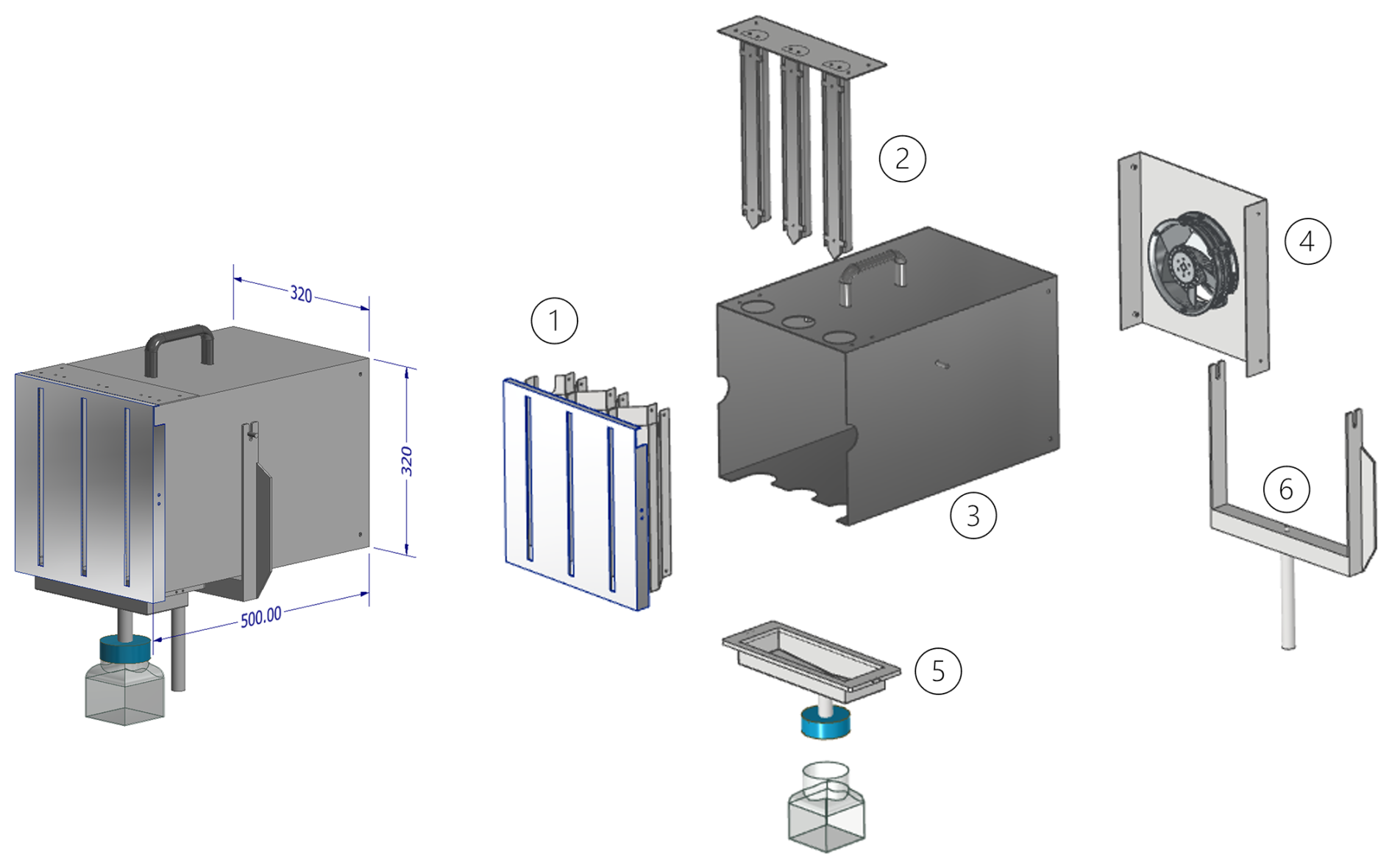
Figure 1 Schematic of the design of the BOOGIE collector. Assembly of the different parts of the BOOGIE collector: (1) front face with the three slots, (2) impaction plates, (3) collector body, (4) rear face with the fan, (5) funnel, and (6) instrument holder.

The cloudy air entered via three rectangular inlets oriented vertically side by side, each 30 cm long and 1.2 cm wide, with 9 cm between them. The droplets were impacted by inertia on aluminium plates located 45 mm behind the air inlets. The inlet width and distance between the inlet and impaction plate were selected to be identical to those of the CWS. The air and smaller non-collected droplets were directed to a shared corridor before the air fan. The collected water flowed to the collection funnel under gravity, and the collection bottle was sterilised.

3.2 Evaluation of the airflow inside the BOOGIE collector

The fan can be modulated at 10 intensities (10 %–100 % of the maximum fan speed). Two ways have been investigated to calculate the airflow through the collector: either by measuring the air inlet velocities at the slots or by measuring the air outlet velocities. First, the air inlet velocities were measured in front of each of the three slots of the BOOGIE collector at different heights (high, middle, and low points) using a hot-wire anemometer, with the velocity modulated according to these 10 values (Fig. S6). The measured velocities varied from 2 to approximately 15 m s⁻¹, with an increase of approximately 1.5 m s⁻¹ per intensity step. The air inlet velocity stabilised at 90 % of the fan speed (corresponding to a measured value of 14 m s⁻¹). By positioning the anemometer identically at each measuring point, the measured velocities at different fan intensities were homogeneous between slots and for the same slot at different heights. However, the positioning of the anemometer is quite sensitive, since a slight displacement can lead to significant measurement deviations. This finding of air velocity heterogeneity at the slots will also be discussed in Sect. 3.3.1.

Therefore, we designed an experiment to measure the airflow at the collector outlet. The airflow rate at the fan outlet was measured using the following procedure. A 3.5 m long PVC pipe with an internal diameter of 154 mm was installed after the fan outlet. This diameter enables the entire flow to be measured without reduction, thus limiting the additional pressure losses generated by the addition of the pipe. A hot-wire anemometer was installed in the tube at 3 m from the fan. The large distance to diameter ratio (greater than 19) minimises disturbances (high turbulence and vortex rates) as the air passes through the axial fan.

The flow velocity profile is measured every 5 mm along the diameter. The flow rate is calculated by summing the average velocity for each ring by the ring area. The flow rate was estimated at 433 m³ h⁻¹ at 90 % of the fan speed. The average velocity in the pipe is found by dividing the flow rate by the cross-sectional area, which corresponds to a velocity of 6.5 m s⁻¹. Based on this velocity, the Darcy–Weisbach formula, and the Moody diagram (with a relative roughness of $\mathrm{2}\times {\mathrm{10}}^{-\mathrm{5}}$), the pressure drop in the pipe is estimated at 10 Pa. As a result, the addition of the pipe has little influence on the flow rate.

The pressure drop in the BOOGIE impactor can be estimated from the fan and flow characteristics. Since the flow rate has been calculated at 433 m³ h⁻¹, the pressure drop compensated for by the fan is estimated at 220 Pa, and consequently the pressure drop in the impactor is around 210 Pa. The variation in density is less than 0.0025 kg m⁻³, i.e. a variation of less than 0.25 %. The flow can be considered incompressible, and conservation of flow volume can be used. The average velocity at the BOOGIE inlet is estimated at 11 m s⁻¹ by dividing the flow by the inlet cross-section of $\mathrm{10.9}\times {\mathrm{10}}^{-\mathrm{3}}$ m². This average velocity differs from the measured velocity at the inlet (14 m s⁻¹) due to the velocity profile at the slots. The measurement corresponds to a maximum velocity.

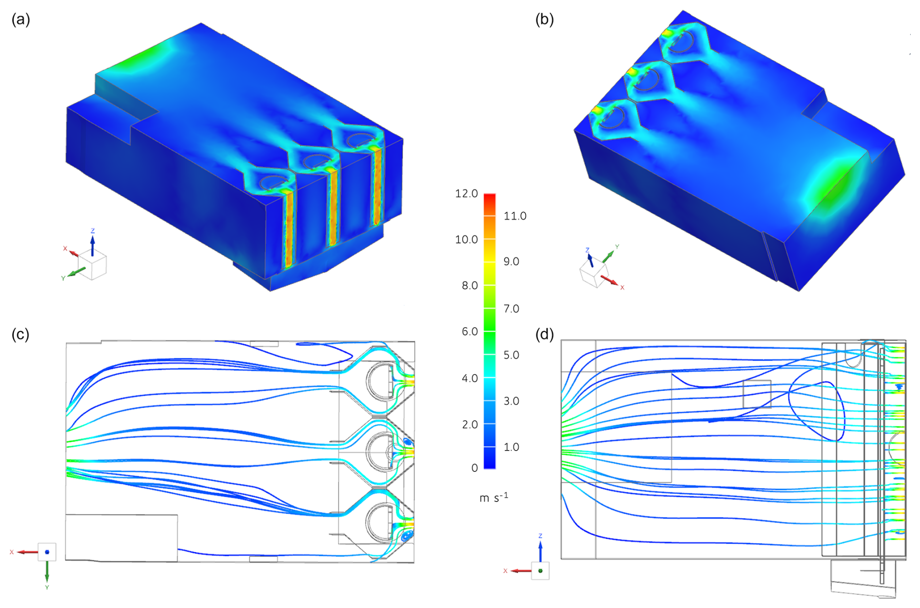
Figure 2 (a, b) Cutting plane in the flow velocity contour (in magnitude) in the case of an air outlet flow velocity of 6.5 m s⁻¹. (c, d) Set of streamlines in the collector (c – right view, d – top view) in the case of an air outlet flow velocity of 6.5 m s⁻¹. The colour code indicates the different air velocity inside the collector.

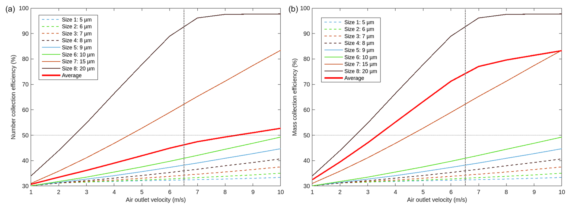
Figure 3 Normalised efficiency of the particle collection regarding the number of droplets (a) and the mass of the droplets (b) for different diameter sizes of particles.

3.3 Performance evaluation

3.3.1 CFD simulations

Flow velocity

Several simulations were performed by modulating the air outlet velocity from 2 to 10 m s⁻¹. Use of the air outlet velocity as the boundary condition avoids imposing direction and velocity distribution at inlet. Figure 2a and b display the flow velocity field inside the collector for an air outlet flow velocity equal to 6.5 m s⁻¹ based on the experimental evaluation presented in Sect. 3.2 (the same for 2 m s⁻¹ in Fig. S7a and b). The air outlet flow velocity equal to 6.5 m s⁻¹ corresponds to a mean air inlet flow velocity equal to 11 m s⁻¹ (1.6 factor). Experimentally, we measured the air inlet flow velocity at a higher value of around 14 m s⁻¹. We present the horizontal cutting planes at the centre of the fan. Regardless of the air outlet velocity, the colour display of the flow velocity contour is identical. We can notice that the velocity simulated close to the slots is heterogeneous, confirming the difficulty of robustly measuring input speed.

Streamlines were also displayed (Figs. 2c, d and S7c, d), with a set of seed points selected randomly on the air inlet faces. They displayed velocity results by showing the path taken by a massless particle. Each point along a streamline is always tangential to the velocity vector of the fluid flow. Again, the streamlines were only slightly modified between the two velocities.

Particle impact tracking

Various radius sizes of particles were injected into the collector at different air outlet velocities. Table S2 lists the number of water droplets for each air outlet velocity and each size of particles (from 5 to 20 µm in diameter) recorded by the solver in front of the three inlets, represented by the three slots. Arbitrarily, approximately 60 000 particles are injected. We calculated the number of injected droplets that impacted the vertical plates among the 60 000 particles; this allowed calculating the normalised efficiency of particle collection for each size of particle and each velocity. Figure 3 reports the efficiency of collection in terms of the number of droplets and the mass of the droplets.

We can observe that as the air outlet velocity increases, so does the collection efficiency for all droplet sizes. For sizes 7 and 8 (more than 15 µm in term of diameter), the number collection efficiencies were > 50 % for velocities higher than 4.5 m s⁻¹. At higher speeds, number collection efficiencies > 80 % were achieved for both size classes. At the maximum speed, a collection efficiency of approximately 50 % was reached for size 6 (10 µm in diameter). Considering the mass of the droplets, the two largest sizes (15 and 20 µm in diameter) naturally represented the largest mass of water collected. Because these two sizes were efficiently collected even at low air velocities, a collection efficiency of 50 % in terms of mass was achieved at 3 m s⁻¹ velocity. At 6.5 m s⁻¹ velocity, the average collection efficiency was approximately 75 % and 47 % in terms of mass and number, respectively.

At 6 m s⁻¹, we observed a slowdown in the overall collection efficiency because the largest drops were already 100 % collected. These results allowed us to estimate the theoretical cutoff diameter at approximately 12 µm when the air outlet velocity is 6.5 m s⁻¹.

These results are subject to limitations and uncertainties related to the modelled physical phenomena. First, the statistical results from the CFD simulations were based on a certain number of particles injected into the computational domain to achieve reasonable computing times. Second, the collection surfaces are supposed to be “ideal”: a droplet that impacts a plate sticks to it; therefore, its transport by gravity to the funnel remains hypothetical. Third, none of the physical phenomena were considered; the simulations were based on the equations of classical fluid mechanics, but other phenomena, such as electrostatics or Brownian motion, may affect the lightest particles. And last, we can also mention that the air outlet velocity estimated experimentally is also subject to uncertainties that could impact the evaluation of the cutoff diameter. However, the performed simulations indicate that the new BOOGIE collector is able to collect cloud droplets, which also confirms that the distance between the air inlet slots and the outlet fan is adequate because it is beneficial for airflow stabilisation.

3.3.2 Field sampling experiments

To evaluate the performance of the BOOGIE sampler, 21 cloud events were collected at PUY station over the period 2016–2024 and the collected water mass as a function of the sampled volume of air was measured (Wieprecht et al., 2005; Demoz et al., 1996). In our database, we selected these events based on the availability of LWC measurements and of the measured mass of the collected water. Table S3 reports various parameters measured during the sampling duration: meteorological parameters (temperature and wind speed) and microphysical cloud properties (liquid water content, LWC_meas, and effective radius, R_eff, every 5 min). These cloud events were in warm conditions between −1 and 11 °C with moderate wind speed (0.2 to 16 m s⁻¹) and LWC from 0.11 to 0.71 g m⁻³. In 2021, three cloud events were sampled using two BOOGIE collectors deployed in parallel (corresponding to S1 and S2 samples). In 2024, a collection with two collectors was systemically done, and several samples were collected consecutively during four cloud events (15, 25, 26, and 29 April 2024). At the end, 39 samples were used to evaluate the BOOGIE collector.

First, we can estimate the cloud water collection rates of BOOGIE equal to 100 ± 53 mL h⁻¹. Water volume is crucial because it determines the biological and chemical analyses that can be performed in the laboratory. The BOOGIE collection rate allows sufficient cloud water to be obtained in a short duration, which is crucial because the origin of the air mass that reaches the collection site can vary in a short time.

Experimentally, we can also evaluate the collected LWC (CLWC_exp) in g m⁻³ (Waldman et al., 1985) as

$$\begin{array}{}\text{(1)}& {\text{CLWC}}_{\exp }={\displaystyle \frac{M}{F\times \mathrm{\Delta }t}},\end{array}$$

where M is the collected water mass (g), F is the sampler airflow (m³ min⁻¹), and Δt is the sampling duration (min).

To evaluate CLWC_exp, we estimated the sampled airflow experimentally at 433 m³ h⁻¹ (7.22 m³ min⁻¹) in Sect. 3.2. In this calculation, we were not able to distinguish the fraction of the air that induced the impaction of droplets as evaluated for the CASCC2 by Demoz et al. (1996). CLWC_exp can be compared with the measured mean LWC_meas for the 21 cloud events (i.e. 39 samples), as shown in Fig. 4.

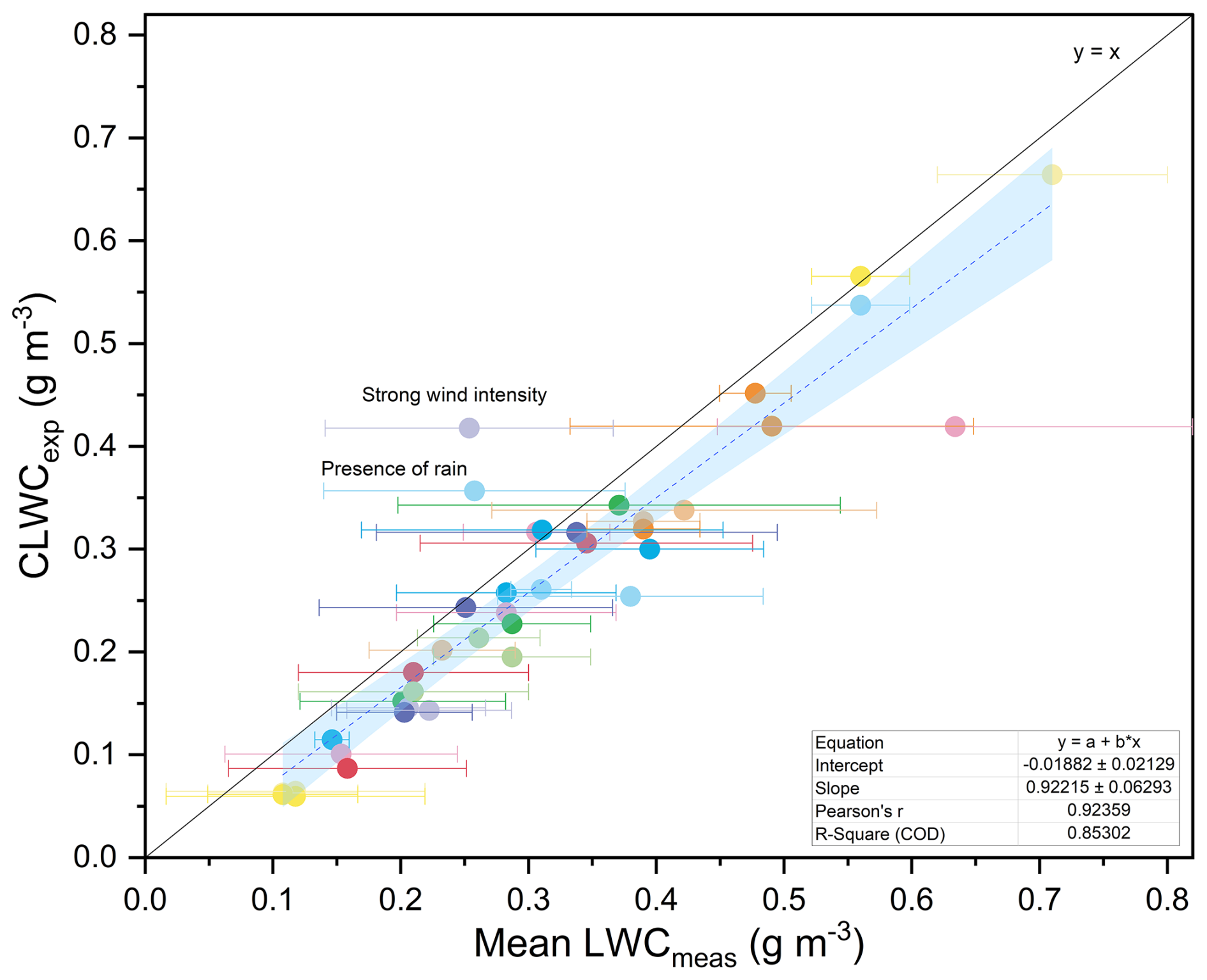
Figure 4 Collected cloud water content CLWC_exp vs. measured LWC_meas (in g m⁻³) for a selection of 21 cloud events sampled at the PUY station. The standard deviation of the measured LWC is indicated. The solid black line represents the y = x function; the linear fit of the experimental data is represented by the dotted blue line, and the blue area denotes the 95 % confidence interval of this fit.

The CLWC_exp and measured LWC_meas were well correlated (the slope of the linear regression was 0.92, and the intercept was −0.02 g m⁻³). Systematic and random deviations from the “theoretical” efficiency are represented by a 1:1 line. Among the 23 cloud samples, only two cloud events presented a CLWC_exp significantly higher than the LWC_meas. Explanations can justify this bias: the cloud event sampled on 3 April 2024 present a high wind speed with a period during the sampling (20 min) where it reached 16 m s⁻¹, and the cloud event sampled on 29 April 2024 was characterised by the presence of fine rain at the end of the sampling period.

The sampling efficiency can be estimated as follows:

$$\begin{array}{}\text{(2)}& \text{Sampling efficiency}\left(\mathit{\%}\right)={\text{CLWC}}_{\exp }/{\text{LWC}}_{\mathrm{meas}}\times \mathrm{100}.\end{array}$$

The average calculated sampling efficiency over 21 cloud events was equal to 73.9 ± 21.4 %. Without considering the two cloud events with significant overestimation of CLWC_exp vs. LWC_meas, the sampling efficiency falls to 69.7 ± 11 %. The sampling efficiency does not appear to decrease when there is a shift to higher LWC_meas. This phenomenon has been observed with other samplers such as the CASCC2, possibly explained by interior collector wall losses for large droplets (Wieprecht et al., 2005).

The mean cloud wind speed and effective cloud droplet radius varied between the cloud events. Figure S8 shows the sampling efficiency vs. the three meteorological and microphysical parameters. The 21 clouds were sampled under conditions typically encountered at PUY for cloud sampling under warm conditions and for different seasons: minimal temperatures > −1 °C with a maximum value of approximately 11 °C and wind speed varying from 0.2 to 16 m s⁻¹. No tendency was observed between the sampling efficiency and temperature, supporting the fact that the collector can be operated over different seasons. The collector's orientation towards the wind is important, particularly under strong wind conditions. Incorrect orientation (i.e. not in front of the wind) could drastically reduce collection efficiency, whereas orientation towards strong winds could improve collection efficiency. For the collected cloud events, we observed that the collection efficiency slightly increased with wind speed; however, the strength of the association was small. At high wind speeds (gusts) near 10 m s⁻¹, cloud droplet sampling can be non-isokinetic, explaining the possible perturbation of collection efficiency. We can notice that four cloud events (corresponding to six samples) were sampled during high wind conditions (more than 11 m s⁻¹). A problem with the orientation of the collector in strong wind conditions can lead to significant gaps in collection efficiency. We cannot rule out the possibility that at some point the collector may not have faced the wind, leading to a reduction in collection efficiency, or that it may have faced the wind at very high intensities, leading to sampling in non-isokinetic conditions and inducing collection efficiencies more than 100 %. This is clearly seen in these four events, which show highly heterogeneous collection efficiencies (from 63.5 % to 164.7 %). The average effective radius varied from 4.6 to 12 µm; there was no correlation between this parameter and the collection efficiency, indicating adequate collection performance of the collector even for smaller droplets.

The collection efficiency calculated herein uses the theoretical total cloud water based on integrated measurement methods (LWC). These estimates must be treated with caution because they are marred by several errors and approximations listed here. These can be the result of the limitations of the instruments themselves (the collector and the PVM probe) and the sampling conditions (wind); with the PVM-100 probe, we cannot optimally capture the time evolution of the LWC because data are recorded every 5 min. Finally, the theoretical sampler airflow used to calculate CLWC_exp can be additionally perturbed by the wind condition. Nevertheless, this first comparison provides a rough estimate of the collection performance of the BOOGIE collector, which appears to be suitable for contrasting environmental conditions.

3.4 Comparison of cloud samplers

A field campaign was conducted at PUY in 2016 to compare the new collector with other commonly used samplers. The BOOGIE collector has been deployed to sample clouds together with the CWS used at the PUY station since 2001 and the CASCC2 (Fig. S9). From 1 June to 2 July, four cloud events were simultaneously sampled using these three samplers. The meteorological conditions and microphysical cloud properties were monitored during the cloud events (Fig. S10). Back trajectories were computed using the CAT model for the four cloud events (Fig. S11). The three samplers were oriented in front of the wind at the beginning of the sampling period; changes in the wind direction were checked during this period, and the orientation of the collectors was modified accordingly.

The prevailing winds during the first two cloud events (1 and 4 June 2016) arrived from the north-northwest and north-northeast directions, whereas the other two (28 June and 2 July 2016) were locally associated with winds coming from the southwest direction. This last event was also characterised by strong wind speeds of up to 14 m s⁻¹ at the end of the sampling time. For the four cloud events, the wind directions did not drastically change during the sampling duration except for 4 June when some fluctuations were observed; however, these were not significant because the wind speed was extremely low (0.2 m s⁻¹). Regarding the microphysical properties, the first cloud event presented lower mean measured LWC (0.15 g m⁻³) in comparison to the others (approximately 0.3 g m⁻³). In contrast, the average radius was highest for the first cloud event (10.8 vs. 4.5–6.6 µm in radius). The temperature corresponded to warm cloud conditions (between 6 and 10 °C), allowing the collection of liquid droplets.

3.4.1 Sampling efficiency

First, the cloud water samplers were compared in terms of sampling efficiency, considering the calculated CLWC_exp and measured LWC_meas (Eq. 2). For the CASCC2, the airflow was evaluated following Demoz et al. (1996) (Sect. 2.3.2). In the calculation presented below, we decided to use the value 348 m³ h⁻¹ without distinguishing the fraction of “sampled air” from the total air entering the collection system. This is motivated by the fact that with the two other collectors we are not able to estimate this fraction. This will allow us to compare collection efficiencies estimated on the same calculation basis. The sampled airflow was evaluated for the CWS, which is a homemade collector that follows the recommendations of Kruisz et al. (1993). As indicated in Sect. 2.3.2, the air inlet flow velocity was measured with a hot-wire anemometer as 13.5 m s⁻¹. Therefore, considering the surface of the entry slot, the sampled air entering the CWS collector was calculated to be equal to 182 m³ h⁻¹ (3.04 m³ min⁻¹). We are aware that this estimation is rough since, as for the BOOGIE collector, the measurement of the airflow velocity at the slot entry is difficult since the positioning of the probe induces biases in the measurement.

Table 1 Information on cloud water collection performed with the BOOGIE, CWS, and CASCC2 samplers for four independent cloud events at PUY. The temperature, wind speed, and R_eff are averaged over the sampling time.

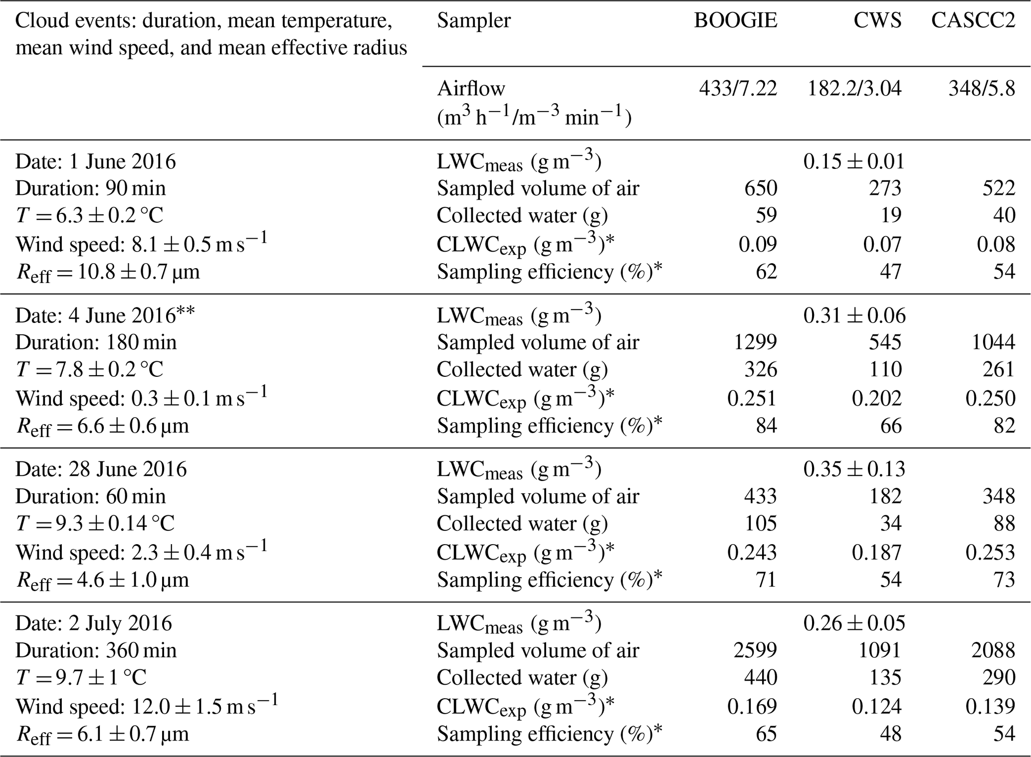
^* The collected LWC (CLWC_exp) is calculated following Eq. (1) and the sampling efficiency by Eq. (2). ${}^{**}$ Fine rain event before the end of sampling.

The CASCC2 and BOOGIE samplers collected between 348 and 433 m³ of air per hour, whereas the sampled volume of air collected by the CWS was markedly lower (around 180 m³ h⁻¹), which explains the lower amount of collected water. The BOOGIE sampler presented a mean water collection rate for the four cloud events of 82 ± 32 mL h⁻¹. This was significantly higher than the rates obtained with the other collectors (CASCC2: 62 ± 30 mL h⁻¹; CWS: 26 ± 11 mL h⁻¹) (t test, p < 0.05). On average, the calculated sampling efficiencies were 70 ± 10 %, 53 ± 9 %, and 66 ± 14 % for BOOGIE, CWS, and CASCC2, respectively. Overall, the three collectors exhibited similar and satisfactory collection efficiencies.

Wieprecht et al. (2005) highlighted that the CASSC2 collection efficiency could be impacted by the loss of droplets off the strands and/or losses inside the collector on the walls, as highlighted in particular for large droplets. This collector appeared to be more affected by the intensity of wind speed, with the lowest collection efficiencies observed for the two windier cloud events. As reported by Kruisz et al. (1993) for CWS and shown in this study for BOOGIE, no correlation of wind speeds with the CLWC_exp of the samplers was found. In the case of the 4 June cloud, the appearance of fine rain during sampling could possibly explain the higher collection efficiency observed for all collectors, as we did not observe conditions such as strong winds that could disrupt the sampling.

Concerning the CASCC2, a sampling efficiency was previously determined during the FEBUKO experiments in the Thüringer Wald (Germany) at 56 ± 17 % (Wieprecht et al., 2005). This sampling efficiency for the CASCC2 seems to be slightly lower than that calculated in the present study. Kruisz et al. (1993) calculated a sampling efficiency of approximately 60 % for the CWS during sampling experiments performed at Mount Sonnblick (Austria) in the same range of order as in the present study. The sampling efficiency depends on environmental conditions and cloud microphysical properties, which differ between collection sites, explaining this variability. The four cloud events were also sampled at PUY under “optimal” conditions (summertime conditions with limited wind speed and sufficient cloud LWC), possibly explaining the efficient collection of the samplers.

3.4.2 Cloud water chemical and biological composition

To compare the three cloud water collectors, we also focused on the chemical compositions of the three cloud water samples collected in 2016. The concentrations of inorganic ions in samples collected with the CWS and CASCC2 collectors (Table S4, Fig. S12) were compared to the concentrations measured in samples collected with BOOGIE using the discrepancy factor (D_f) calculated using Eqs. (3a) and (3b).

$$\begin{array}{}\text{(3)}& D_{\mathrm{f},\mathrm{CWS}}={\displaystyle \frac{C_{\mathrm{BOOGIE}}-C_{\mathrm{CWS}}}{\left(\frac{C_{\mathrm{BOOGIE}}+C_{\mathrm{CWS}}}{\mathrm{2}}\right)}}\end{array}$$

$$\begin{array}{}\text{(4)}& D_{\mathrm{f},\mathrm{CASCC}\mathrm{2}}={\displaystyle \frac{C_{\mathrm{BOOGIE}}-C_{\mathrm{CASCC}\mathrm{2}}}{\left(\frac{C_{\mathrm{BOOGIE}}+C_{\mathrm{CASCC}\mathrm{2}}}{\mathrm{2}}\right)}}\end{array}$$

Here, C_BOOGIE is the concentration of ions measured in samples collected with BOOGIE, and C_CWS and C_CASCC2 are the concentrations of ions measured with CWS and CASCC2, respectively.

Figure 5 Histograms presenting discrepancy factors (D_f) between BOOGIE and CWS and between BOOGIE and CASCC2 calculated using anion and cation concentrations for the three cloud samples. The dashed lines represent the analytical error, whereas the solid line represents the 50 % discrepancy.

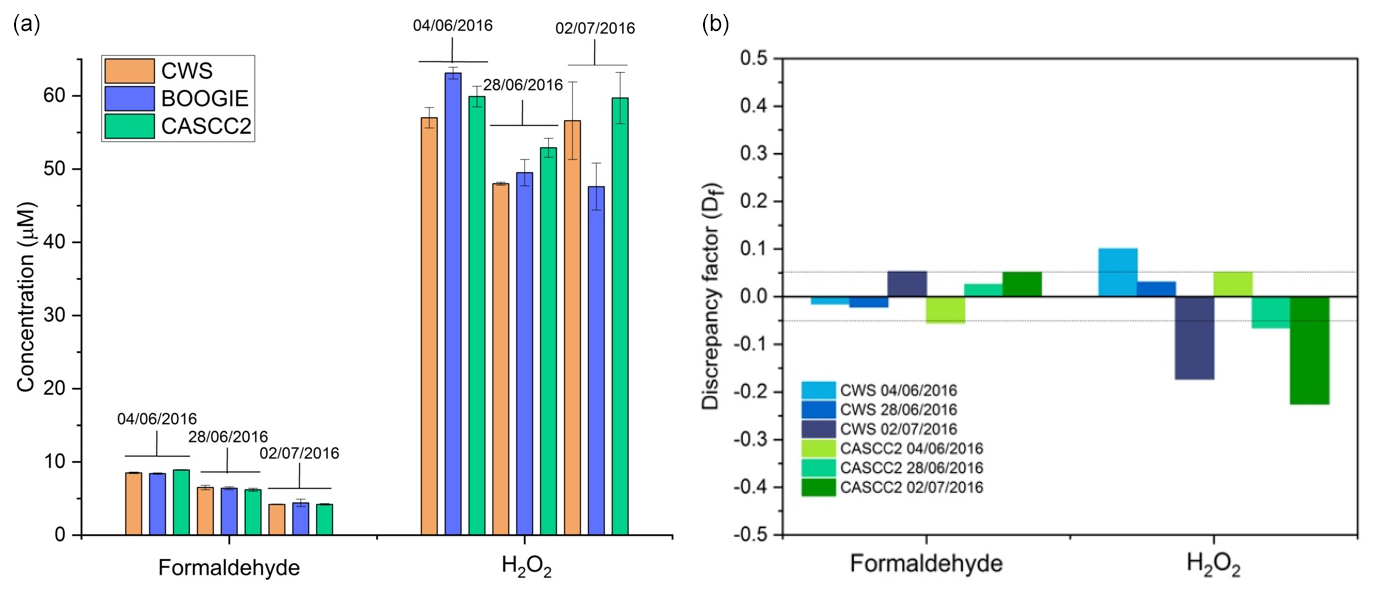
Figure 6 (a) Histograms presenting the formaldehyde and hydrogen peroxide concentrations for the three cloud samples collected using CWS, BOOGIE, and CASCC2 in parallel. The error bars correspond to the standard deviation. (b) Histograms presenting discrepancy factors (D_f) between BOOGIE and CWS and between BOOGIE and CASCC2. The dashed lines represent the analytical error.

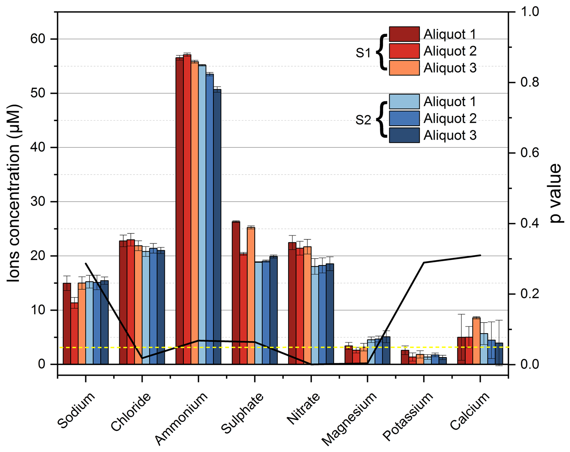
Figure 7 Histograms presenting the concentrations for a specific cloud sampled on 8 July 2021 at PUY with two BOOGIE collectors. This time, three aliquots were analysed twice (error bars) using ion chromatography. The p values are indicated with the black line, and the dashed yellow line indicates the threshold of p = 0.05.

Figure 5 shows the estimated D_f,CWS and D_f,CASCC2 for anions and cations for cloud samples. The horizontal dashed lines represent the analytical error in the measurement, which is comparable with D_f,CWS on 2 July 2016 for sulfate, nitrate, chloride, and ammonium and D_f,CASCC2 on 28 June and 2 July 2016 for nitrate, sulfate, chloride, and sodium. The other D_f values were higher, but generally < 0.5, which could represent a good comparability of the cloud collectors because the chemical composition of cloud condensation nuclei may be inhomogeneous. A higher variability by a factor of 3 to 6 was observed for the magnesium and potassium ions, but they also present a lower concentration under 15 and 8 µM, respectively (Fig. S12). For the most concentrated ions ammonium (over 150 µM) and nitrate (over 50 µM), their concentrations are comparable between the samplers.

At first glance, concentrations with the CASCC2 appear to be slightly higher, but not for all ionic species and not for all the cloud events. These three samplers present specific designs and surfaces of collection (plate for BOOGIE and CWS vs. strands for CASCC2), leading to different estimated cutoff diameters (12 µm for BOOGIE, 7.5 µm for CWS, and 3.5 µm for CASCC2) and possibly to differences in the chemical composition of the samples.

Formaldehyde and hydrogen peroxide concentrations have also been measured in samples obtained with the three collectors. Concentrations and discrepancy factors between collectors are presented in Fig. 6. These results are consistent with what was observed with the ionic content because the collectors indicate D_f values mostly within the analytical error and maximum measured D_f values < 0.5.

To further evaluate BOOGIE, two identical collectors were installed at the PUY station in 2021 to check for differences in the chemical composition of cloud waters collected in parallel. For clouds on 8 July 2021, chemical measurements were performed in triplicate to analyse the statistical differences (Fig. 7, Table S5). The error bars depict the analysis error, which is higher than the discrepancy between the BOOGIE collectors for sodium, potassium, calcium, and chloride. The solid black line represents the p value obtained for the t test (right y axis); if the p value is < 0.05, represented in the plot by the dashed yellow line, the difference between the two BOOGIE collectors is significant, as observed for magnesium, nitrate, and chloride. Nevertheless, the difference was not significant for sodium, ammonium, potassium, calcium, and sulfate, indicating good reproducibility of sampling with the BOOGIE collectors.

Given the uncertainties in laboratory measurements and the possible intrinsic variability of the chemical composition within the cloud system, we can reasonably argue that the chemical compositions of the collectors are comparable. Schell et al. (1992) compared two single-stage cloud impactors with different designs and highlighted the large differences between the ionic compositions of the samples. These differences have been hypothesised to be related to different microphysical properties of the sampled clouds that induced bias in the collection: smaller droplets can be sampled with a lower cutoff diameter of the collector, and a lower LWC can eventually induce some evaporation of the smaller droplets. The three cloud events presented “stable” microphysical properties during their collection period (Fig. S9). This could explain the good agreement between the collectors in terms of their chemical composition. Wieprecht et al. (2005) compared the chemical composition of cloud water collected with a low-volume single-stage slit jet impactor and with the CASCC2 string collector and reported 8 %–15 % differences in the solute ionic mass in cloud water, in the range observed in the present study (4 %–35 % differences, average of 12 %) between the three collectors.

The microbial energetic state given by the in-cell ATP and ADP concentrations from each cloud sample was assessed during the intercomparison campaign (see the Supplement for a description of the protocol). The ATP $/$ ADP ratio gives the energetic stress of the cloud water microbiota; a ratio < 0.6 indicates a good energetic state, 0.6 to 1 a medium one, and > 1 a low energetic state. The measured ratios are listed in Table S6. The ATP $/$ ADP ratio ranged from 0.2 to 0.4, revealing a good energetic state of microflora for each sample. The measured ATP $/$ ADP ratios were similar for the cloud water samples from the three collectors. Thus, we argue that the three samplers could be considered non-stressful and suitable for cloud microbiota collection.

4 Conclusions

This study presented a new cloud collector called BOOGIE. This single-stage collector allows cloudy air containing aqueous droplets to be drawn through three air inlets in the form of vertically oriented slots. The cloud droplets were collected using vertical plates placed behind the slots, allowing them to be impacted. They then flowed by gravity along the plates, fell into a funnel, and ended up in a sterilised glass bottle. It was made of aluminium but can be manufactured from other materials, such as plastic materials like nylon or PTFE to investigate transition metal ions in cloud waters. The cloud collector can be connected to the mains or run on batteries (12 V voltage); thus, the collector can be operated on its own power during field measurement campaigns for at least 4 h using a 2 kg small battery. Parts of the sampler were removed for cleaning; the front face, impaction chamber, funnel, and glass bottle were sterilised in an autoclave. This allowed for the characterisation of the biological content of the sampled clouds (biodiversity, concentration, and viability and activity) (Vaïtilingom et al., 2012). Biological and chemical collector blanks were easily prepared by spraying Milli-Q water onto the collection plates and collecting the water flowing into the collection glass bottle.

CFD simulations were performed to investigate how the collector captured cloud droplets. First, considering the 3D structure of the collector, some turbulence was simulated inside the collector, which was reassuring. Different sizes of cloud droplets were injected into the collector to simulate their impacts on the collection plates. This theoretical study indicates that on average, for all droplet sizes (radius from 2.5 to 10 µm), the average collection efficiencies of > 50 % in terms of numbers were achieved at air outlet velocities > 8 m s⁻¹. A collection efficiency of approximately 50 % was reached for droplets 5 µm in radius that gave us an estimate of the 50 % cutoff diameter of the collector (approximately 12 µm). This estimate seems higher than the cutoff diameters of other cloud samplers (more in the range between 3.5 and 10 µm in diameter). However, comparisons of cutoff diameters between samplers are difficult because these estimates are made using different methods; in particular, the theoretical collection efficiency often considers the Stokes number (Demoz et al., 1996).

Based on the 21 cloud events sampled at the PUY station, a mean water collection efficiency was calculated as 100 ± 53 mL h⁻¹ for clouds presenting various microphysical cloud properties: the mean LWC was between 0.11 and 0.71 g m⁻³ and the mean effective radius R_eff was between 4.6 and 11.8 µm. This made it possible to obtain sufficient water volumes over short periods for targeted chemical and biological analyses. This is crucial for minimally integrating the cloud properties in space and time. Methodological developments in recent years have made it possible to assess the organic composition and biodiversity of this aqueous environment using non-targeted methods (Rossi et al., 2023; Bianco et al., 2018). This requires large volumes of cloud water (hundreds of millilitres or even litres of water), which can be collected rapidly using the new collector alone or by duplicating it.

Considering the measured LWC, LWC_meas, the sampling efficiency of this new collector was estimated at 69.7 ± 11 % over the same set of cloud events collected at PUY. No significant tendency in the collection efficiency was observed as the wind speed increased over the range of variation between 0.3 and more than 15 m s⁻¹, and definite variability in the collection efficiency was observed in high wind conditions. No significant correlation was observed between the efficiency and mean measured effective radius. A low-LWC cloud event would likely present a greater proportion of liquid water residing in smaller droplets; therefore, for a low LWC, we expected the collection efficiency to diminish owing to the cutoff diameter. However, this decrease was not observed in the cloud samples. Additional measurements of droplet size distribution during sampling would be beneficial for clarifying this issue.

We compared the collection efficiency and chemical compositions of the BOOGIE collector with two collectors that are commonly used by the scientific community to study cloud composition and environmental variability: the CWS and the CASCC2. For the four studied cloud events, the BOOGIE collector presented an elevated water collection rate of 82 ± 32 mL h⁻¹ (CASCC2: 62 ± 30 mL h⁻¹; CWS: 26 ± 11 mL h⁻¹). This can be explained by the increased volume of cloudy air entering the new collector. On average, the calculated sampling efficiency was 70 ± 10 % for BOOGIE, in the same range as that for CASCC2 and CWS. The chemical and biological compositions measured in the samples collected by the three collectors can be evaluated as comparable; however, some differences can be highlighted, which can be explained by the design of the collector, type of collection, and inhomogeneous chemical composition of the cloud condensation nuclei.

This BOOGIE collector is designed for use in field campaigns and long-term observatory sites. It contributes to the evaluation of the complex cloud water bio-physicochemical composition and to the analysis of its environmental variability; it allows a sufficient volume of water to be collected to characterise the chemical and biological transformations occurring in it. This will help better constrain detailed cloud chemistry models that need to be validated (Barth et al., 2021). For future development, our team aims to reduce the size and weight of the collector such that it can be installed under a native balloon. The second development concerns the automation of this collector to initiate collection remotely and increase the sampling frequency. Finally, we aim to conduct intensive campaigns in the framework of the ACTRIS Cloud In Situ network to compare the collectors used by the scientific community at other measurement sites.