Factors limiting contrail detection in satellite imagery

Contrails (ice clouds, originally line-shaped after initiation by aircraft exhaust) provide a significant warming contribution to the overall climate impact of aviation. This makes reducing them a key target for future climate strategies in the sector. Identifying pathways for contrail reduction requires accurate models of contrail formation and life cycle, which in turn need suitable observations to constrain them. Infrared imagers on geostationary satellites provide widespread contrail observations, with sufficient time resolution to observe the evolution of their properties. However, contrails are often narrow and optically thin, which makes them challenging for satellites to identify. Quantifying the impact of contrail properties on observability is essential to determine the extent to which satellite observations can be used to constrain contrail models and to assess the climate impact of aviation.

In this work, contrail observability is tested by applying a simple contrail detection algorithm to synthetic images of linear contrails in an otherwise clear sky against a homogeneous ocean background. Only (46±2) % of a modelled population of global contrail segments is found to be observable using current 2 km resolution satellite-borne imagers, even in this maximally observable case. By estimating the radiative forcing of individually modelled contrails, it is found that a significantly higher portion of contrail forcing is detectable using the same 2 km resolution imager – (72±2) % of instantaneous long-wave (LW) forcing – because more easily observable contrails have a larger climate impact. This detection efficiency could be partly improved by using a higher-resolution infrared imager, which would also allow contrails to be detected earlier in their life cycle. However, even this instrument would still miss the large fraction of contrails that are too optically thin to be detected.

These results support the use of contrail detection and lifetime observations from existing satellite imagers to draw conclusions about the relative radiative importance of different contrails under near-ideal conditions. However, there is a highlighted need to assess the observability of contrails where the observation conditions may vary by application. These observability factors are shown to change in response to climate action, demonstrating a need to consider the properties of the observing system when assessing the impacts of proposed mitigation strategies.

1 Introduction

Contrail cirrus is recognised as a significant driver of aviation's climate warming: Lee et al. (2021) suggest it is the cause of more than half the radiative forcing of the sector. Contrail forcing is warming in the long wave (LW), via the cloud greenhouse effect, and cooling in the short wave (SW), via the cloud albedo effect (Meerkötter et al., 1999). This strong anthropogenic radiative forcing provides impetus for action on contrail mitigation and research.

Early estimates of the radiative forcing due to contrails (e.g. Meerkötter et al., 1999; Meyer et al., 2002) relied on the scaling of radiative transfer simulations to the coverage of linear contrails – measured regionally in satellite observations via either manual identification (Bakan et al., 1994) or using algorithms for detecting line-shaped ice clouds (Mannstein et al., 1999). The observations use infrared images – particularly split-window brightness temperature images (Lee, 1989) – which highlight optically thin ice clouds with small crystals against the surface and background liquid clouds. Both the strong signal and the linearity of the object are used to detect the presence of a line-shaped contrail.

Historically, geostationary satellites did not offer high enough spatial resolution to detect contrails, as illustrated by the use of imagers on low Earth orbit (LEO) satellites for contrail detection (Mannstein et al., 1999; Duda et al., 2013; Vázquez-Navarro et al., 2015). Geostationary observations have the advantage of continuous observation of the same scene with a single instrument, sufficiently time-resolved to observe contrail evolution. Some studies, including Vázquez-Navarro et al. (2015), identified contrails in LEO satellite imagery before tracking them in geostationary images. Some contrails detected in LEO imagery were not observable in simultaneous geostationary images, demonstrating an instrument dependence of observability. Gierens and Vázquez-Navarro (2018) used statistical approximations to derive that contrails tracked using this technique may be observable for less than half their lifetime, due to unobserved parts of the evolution both before and after observation.

Several recent observational studies have demonstrated the ability to detect contrails using modern geostationary satellites (GOES-R series and Himawari 8), including Zhang et al. (2018), Meijer et al. (2022), and Ng et al. (2023). These modern satellites have infrared bands used for contrail detection with approximately 2 km resolution at nadir. Initial detection in geostationary images has been found to occur 10–45 min after formation (Chevallier et al., 2023; Gryspeerdt et al., 2024; Geraedts et al., 2024), indicating that contrails are unobservable for at least the earlier part of their evolution. Although the contrails are assumed to have small radiative impact during this time, which could be estimated if accurately matched to a generating flight, the delayed onset is an obstacle when attempting to attribute observed contrails to specific aircraft (as was an aim of each of these studies). Each of these studies uses convolutional neural nets to detect the contrails. These rely on datasets of extended line-shaped contrails used as “training data” to produce an algorithm that is able to detect linear contrails.

Early studies of linear contrail detection in satellite imagery centre discussions of detection efficiency around the background conditions: surface inhomogeneities driving detection efficiency losses or false positive overdetections (Mannstein et al., 1999; Meyer et al., 2002, 2007; Minnis et al., 2005; Palikonda et al., 2005). Later, Kärcher et al. (2009) established that the properties of the contrail also affect its observability. It was shown that the observed distribution of contrail optical thickness differs from the distribution produced by a model (CCSIM, an analytical model shown to be consistent with large-eddy simulations). The observations underestimated the occurrence of optically thin contrails (with optical thickness <0.2), relative to the model – an empirically inferred optical-thickness-dependent detection efficiency was able to reconcile model with observation. Although optical thickness ought to be a good predictor of contrail observability, underlying microphysical properties (such as particle size and concentration) will have individual effects on the observability of contrails, depending on the techniques used for their detection (Yang et al., 2010).

The adoption of convolutional neural net algorithms brings with it a new set of limitations to discuss regarding their detection efficiency. These algorithms are typically trained and benchmarked against datasets of contrails identified by humans in satellite imagery; such datasets are also used as “training data” (Meijer et al., 2022; Ng et al., 2023; Gryspeerdt et al., 2024). Using human-labelled datasets as a benchmark neglects the cases which are unobservable by human labellers (which are likely also unobservable by algorithmic methods), potentially leading to overestimated detection efficiency.

A concept known as “satellite simulation” (e.g. Bodas-Salcedo et al., 2011) can aid in the essential analysis of contrail observability while not depending on the observational limits of a human labeller. These analyses should seek to account for varying instrument properties, the wide variety of contrail micro- and macrophysical properties, and the background conditions; it is not clear that a simple optical depth threshold is suitable for this purpose.

Well-understood observations are required for a large number of reasons, for example, to validate models like the contrail cirrus prediction (CoCiP) model (Schumann, 2012). CoCiP produces predictions which generally align with observations regarding the order of magnitude and principle age dependencies for micro- and macrophysical properties (Schumann et al., 2017). Planning for in situ observations is informed by CoCiP applied to forecast data (Voigt et al., 2017). The model has also been used to consider potential consequences of lower non-volatile particulate emissions following climate action, such as due to the adoption of sustainable aviation fuel (SAF) (Teoh et al., 2022b). CoCiP is based on simple, well-understood criteria for formation and persistence, described in Schumann (1996). Most fundamentally, this is driven by the Schmidt–Appleman temperature threshold for mixing cloud formation. The properties of the formed contrail are then allowed to evolve, subject to ice water content changes in response to ambient supersaturation, diffusion, and particle number loss processes (Schumann, 2012). Meteorological input limits the predictability of persistent contrail formation, particularly uncertainty in relative humidity values at flight altitudes (Gierens et al., 2020; Agarwal et al., 2022). Model adaptations, such as the correction of input relative humidity from meteorology (Teoh et al., 2022a) or alterations to contrail processes like ice crystal formation and loss mechanisms (Schumann et al., 2017), require well-understood contrail observations for validation.

Beyond model validation, other applications have a varied range of specific observational needs. For example, applications include climate monitoring and operational tactical avoidance (action taken in response to current conditions to mitigate the impact of individually forecast contrails; Chevallier et al., 2023; Sausen et al., 2023; Geraedts et al., 2024). These applications require observation of as high a proportion of strongly forcing contrails as possible (at least at some point in their evolution) and often need to match contrails to flights or take quick action, so observation as quickly after formation as possible is required. The planning of experimental trials seeking to analyse changes to contrail formation or persistence will benefit from an understanding of the dependence of observability on the properties of contrails and the surrounding conditions so that they can be confident that unobserved contrails are indeed unformed contrails (Molloy et al., 2022).

This study establishes limits of observability for the automated detection of line-shaped contrails as a function of the contrail properties, independently from models. The detectability of linear contrails is tested in otherwise clear-sky synthetic satellite images by applying a contrail detection algorithm. The derived observability threshold will then be compared with CoCiP-modelled populations of global contrails and their estimated radiative forcing (from Teoh et al., 2024a), and the consequences for a range of applications will be considered. In Sect. 2, key components of the observability analysis are described, including the simulated contrail images and the models used to create them (Sect. 2.1), the line-filtering contrail detection algorithm (Sect. 2.2), and the modelled population of global contrails (Sect. 2.3). Observability assessments are made in Sect. 3, including varying single parameters (Sect. 3.1) and deriving an observability threshold against the key observability-driving properties (Sect. 3.2) – properties which form a parameter space in which the population of contrails is shown to be well resolved (Sect. 3.3). The derived observability threshold is finally applied to the properties of contrails modelled to form in Sect. 4, resulting in estimates of the observable fraction (Sect. 4.1), the evolution of this observability with contrail ageing (Sect. 4.2), the lifetime radiative impact of contrails based on their observed lifetime (Sect. 4.3), and the changing observability as climate action is taken (Sect. 4.4).

2 Algorithms and data

2.1 Simulated contrail images

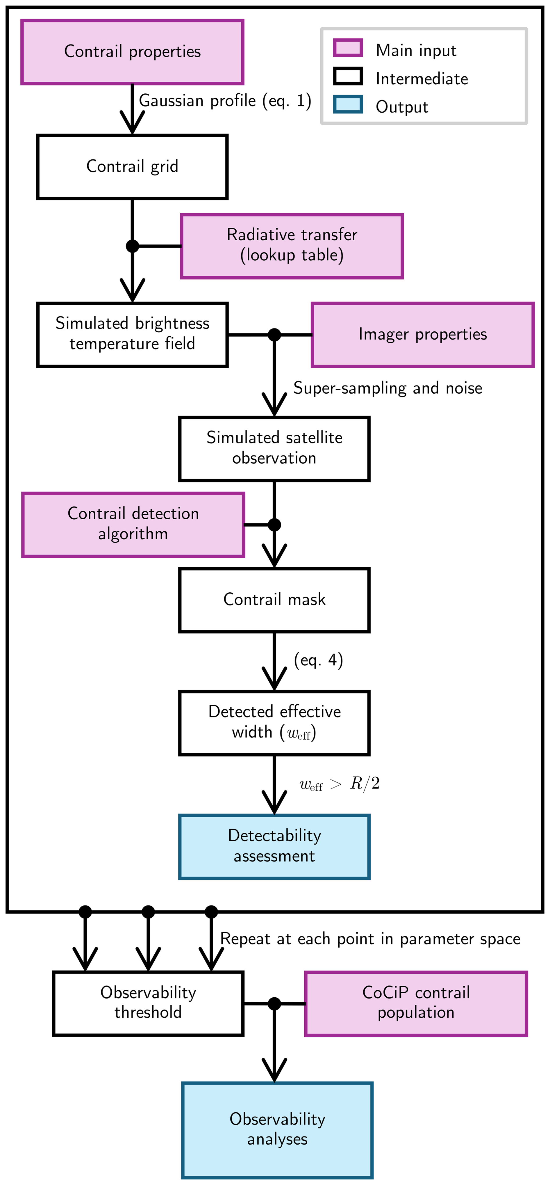
Figure 1 Schematic of the process for deriving contrail detection efficiency by application of a contrail detection algorithm to synthetic observations of a single contrail, using a specific imager and contrail detection algorithm and a pre-calculated radiative transfer lookup table.

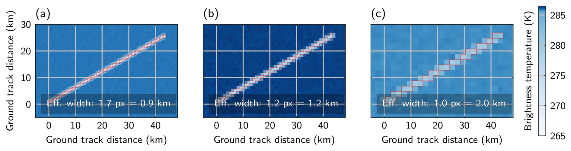
Figure 2 Example simulated observations of 50 km long contrails, imitating imagers with (a) 0.5 km, (b) 1 km, and (c) 2 km surface spatial resolution. Values are brightness temperatures as observed using the profile of the GOES-ABI band 14 (centred on 11.2 µm). The red line denotes the contrail mask detected. Note the skewed colour scheme intended to simultaneously highlight imager noise and decreased peak brightness temperature with the coarsening resolution. Image-to-image variability is given by a simulated calibration error (sampled for each realisation from a Gaussian with a standard deviation of 0.2 K), and pixel-to-pixel variability is given by the NEdT (sampled for each pixel from a Gaussian with a standard deviation of 0.03 K).

The observability of a contrail segment is tested by running a contrail detection algorithm over simple simulated radiance fields of synthetic straight-line contrails above a clear-sky ocean scene. The process is outlined in the schematic, Fig. 1.

Test contrails are constructed as 150 km long cloud segments, with an ice water path (IWP) which varies across the contrail in a Gaussian profile. The profile has the form

$$\begin{array}{}\text{(1)}& \text{IWP}(s;{\text{IWP}}_{\mathrm{0}},B)={\text{IWP}}_{\mathrm{0}}\sqrt{{\displaystyle \frac{\mathrm{4}}{\mathit{\pi }}}}\exp \left(-{\displaystyle \frac{\mathrm{1}}{\mathrm{2}}}{\displaystyle \frac{s^{\mathrm{2}}}{B^{\mathrm{2}}/\mathrm{8}}}\right),\end{array}$$

describing variations from the characteristic “contrail IWP” (IWP₀) across the distance (s) perpendicular to the contrail's length, given the width of the specific test contrail (B). This is consistent with the optical depth profile used for CoCiP-modelled contrails, described in Schumann (2012). Alongside B and IWP₀, the effective radius (r_eff) is another characteristic contrail property (describing the size of constituent ice crystals). Each synthetic contrail is assumed to have constant r_eff. In reality, contrails are not straight lines, and their properties and evolution may vary along their length. The consequence of such variations is considered in this work by using the detectability of these test contrails to inform the observability of modelled contrail “segments”; the overall contrail's properties may vary from segment to segment.

A 1D radiative transfer simulation using the US standard atmosphere is run at each point in the test contrail on a 0.25 km grid to produce a radiance field (at “high-resolution” relative to satellite imager output), from which brightness temperatures are calculated. The DISORT algorithm (Buras et al., 2011) was used for radiative transfer calculations, as implemented in the libRadtran library (Emde et al., 2016), with the pyLRT Python wrapper (Gryspeerdt and Driver, 2024) used to perform the simulations. The ice water content and size distribution are assumed uniform across the contrail depth. When r_eff>5 µm, the contrails are parameterised using the Yang et al. (2013) parameterisation as distributed with libRadtran, using smooth droxtal (faceted spheroid) habits. The lower limit on r_eff is a limit of this parameterisation. To simulate contrails with smaller ice crystals, absorption coefficients were calculated using the “mie” package (also distributed with libRadtran) for spherical ice crystals with a gamma distribution of particle radii consistent with the libRadtran microphysics implementation. The viewing zenith angle has been taken to be zero, introducing an assumption that observation occurs near the satellite's nadir. The surface is assumed to have unit thermal emissivity (similar conditions to the ocean), and the surface temperature is treated as 15 °C (a property of the temperature profile). GOES-ABI imager bands are simulated using the REPTRAN representative wavelength parameterisation (Gasteiger et al., 2014).

For computational efficiency, a lookup table of brightness temperature values for a comprehensive range of contrail physical properties was used to produce the simulated brightness temperature fields. The radiative transfer lookup table is based on a parameter space grid, linearly spaced in IWP (between 0 and 100 g m⁻²), r_eff (between 0.1 and 80 µm), contrail depth (between 50 and 1500 m), and altitude (between 6 and 13 km). Linear spacing of the lookup table includes more gradual variations in simulated radiances than a logarithmically spaced parameter grid, so it is better suited for interpolation where required.

The high-resolution simulated brightness temperature field is then processed to simulate the properties of a given imager, coarsening the resolution and applying measurement noise. The brightness temperature grid is coarsened to a grid given by the imager's resolution, using a conservative local-mean downgridding technique (to integer multiples of the high-resolution grid). A Gaussian noise with standard deviation equal to a noise-equivalent temperature deviation (NEdT) of 0.03 K is applied to simulate the pixel-to-pixel uncertainty – approximately equivalent to the GOES-ABI NEdT based on on-orbit tests of GOES-16 (NASA, 2019; Wu and Schmidt, 2019). Multiple realisations of the brightness temperature field are produced, each offset with a single calibration error sampled from a 0.2 K wide Gaussian – representative of the image-to-image uncertainty of the GOES-ABI imager (NASA, 2019). Examples of such synthetic brightness temperature fields are shown in Fig. 2.

Radiative transfer modelling of contrails has previously been performed by Schumann et al. (2012) and Wolf et al. (2023). Both these previous works similarly use libRadtran (Emde et al., 2016) to perform calculations. Each use similar ice cloud parameterisation settings to this work, with Schumann et al. (2012) using an earlier set of scattering properties. The previous works similarly suffer from a lack of scattering properties for small crystals, and the work by Schumann et al. (2012) turns to Mie calculations for this purpose, as is done in this work. For larger crystals, each of the two previous works chooses to use a range of different habits which may be found in contrails – this was omitted here with the aim of choosing a habit that was consistent with the Mie calculations. Similarly, the other works use a range of atmospheric profiles. The approach taken here is aligned with the aim of considering an idealised case to provide an upper limit of the detectability; variation in habit mixtures and atmospheric profiles will add further variability to the detection efficiency achievable in practice. The other works have additional considerations for solar radiation, including solar zenith angle variations, which are neglected in this work due to the focus on thermal radiation for the detection algorithm used.

2.2 Contrail detection algorithm and observability criteria

A simple convolutional filtering contrail detection algorithm is applied to the images. The detection algorithm used is based on the implementation of the Mannstein et al. (1999) algorithm, as implemented by McCloskey et al. (2021). This is a line-filtering algorithm, applied on infrared brightness temperature fields. Brightness temperature (using the 11.2 µm band of the GOES ABI instrument) and brightness temperature difference (between the 10.3 and 12.3 µm bands of the same instrument) fields are used for contrail detection. The fields are low-pass-filtered, differenced from a smoothed version to extract the signal, normalised, and clipped of extreme values. A threshold is applied to each of the two fields, along with a combined field convolved with line filters in a range of different directions. For the McCloskey et al. (2021) implementation, the thresholds have been tuned on a human-labelled dataset, establishing the contrails detected using this algorithm as representative of those observable by human labellers. The detection algorithm produces a binary mask of pixels detected as being “contrail”.

The algorithm was minimally adapted in this work to relieve some emergent issues. It was found to selectively omit contrails aligned with the dimensions of the simulated imager grid, a result of using the r-squared statistic as a test for linearity. A linearity score was devised to replace the r-squared statistic,

$$\begin{array}{}\text{(2)}& {\mathit{ϵ}}^{\mathrm{2}}=\mathrm{1}-{\displaystyle \frac{\sum d_{⟂}^{\mathrm{2}}}{\sum d_{\parallel }^{\mathrm{2}}}},\end{array}$$

where d_⟂ is the perpendicular distance to a pixel from a linear fit to the masked points, d_∥ is the distance between a masked pixel and the midpoint of the line, and sums act over each of the pixels in the detected area. ϵ is the eccentricity of an ellipse whose semi-major and semi-minor axes are the mean d_∥ and d_⟂, respectively. This relieves the dependence on axes arbitrarily chosen relative to the contrail.

Detected contrails were also checked for their alignment with the simulated contrail. Regions whose orientations differed from the simulated contrail by ±30° are neglected. This removes artefacts where the “end” of the contrail, but not the main body of the contrail, is detected. This is a result of the contrail profiles terminating suddenly, producing a regional gradient in brightness temperature fields, which is picked out by the detection algorithms used in this work. This only arises for very wide, optically thick simulated contrails, due to their physically unrealistic profiles; such a condition would never be needed in operations on real observations.

The algorithm produces a mask of contrail pixels from an image, of area

$$\begin{array}{}\text{(3)}& A_{\text{mask}}=N_{\text{px}}{R}^{\mathrm{2}},\end{array}$$

where N_px is the number of masked pixels and R is the imager resolution. The presence of a contrail is accurately detected if the mask is made up of at least 1 pixel along the length of the contrail. It is useful to regard the width of the area detected as a contrail because an imager is only able to detect an area in units of pixels. We define the “effective width” as

$$\begin{array}{}\text{(4)}& w_{\text{eff}}={\displaystyle \frac{A_{\text{mask}}}{l}}\Rightarrow {\displaystyle \frac{w_{\text{eff}}}{R}}={\displaystyle \frac{N_{\text{px}}}{l/R}}.\end{array}$$

A 1-pixel effective width (w_eff=R) corresponds to a minimally detected contrail along the whole length (l) of the contrail. For each simulated contrail detection attempt, a threshold $w_{\text{eff}}>R/\mathrm{2}$ is applied, such that a detection along most of the length, but not necessarily all of it, is accepted. This minimally restrictive condition ensures that very narrow contrails whose ends are omitted from the mask are not penalised as failed detections.

2.3 The distribution of “real” contrail properties

A reference population of contrails and their properties is needed to analyse whether the most climatically relevant contrails are observable: those which form and persist and those which cause the most radiative forcing. To avoid the observational biases in the population of contrails, a modelled inventory of contrails is used.

The CoCiP-derived contrail dataset of Teoh et al. (2024a) provides a global inventory of contrail segments globally at 5 min intervals, derived from air traffic data. These segments are the result of the application of CoCiP for flights in 2019–2021, produced using the pycontrails implementation of the model in Python (Shapiro et al., 2023), including radiative forcing estimates based on the parameterisation of Schumann et al. (2012). Air traffic is based on the GAIA emissions inventory (Teoh et al., 2024b), which showed good agreement with other flight inventories and showed only a small deficit compared to major airport statistics. This population of contrails should not be expected to match observations on a flight-by-flight basis. It is produced using the ERA5 meteorological reanalysis, which has difficulty producing accurate ice supersaturation fields at flight altitudes (Gierens et al., 2020). However, it is assumed that the statistics of this population are aligned with the population of actual contrails.

Two populations are used for different parts of this work:

1. The “instantaneous” sample, constructed from global contrail datasets at 114 time steps randomly sampled through 2019, with minimum separations of 24 h. This is approximately 14 million contrail segments in total. The timestamps are well distributed seasonally and throughout the day, so they are representative of seasonality and the diurnal cycles of meteorology, forcing, and air traffic.

2. The time-resolved dataset, wherein the properties of all contrail segments that formed in a 24 h period between 12:00 UTC on 6 and 7 July 2019 were tracked for their whole lifetime, up to 12 h after their formation (at which time they would be removed by CoCiP). Around 1 million contrail segments are formed in the 24 h window, forming a dataset of 34 million segments as they evolve.

The contrail data are analysed as a set of contrail segments – partial lengths of contrail which form over 5 min intervals. This supports the analysis of geometrically extended contrails with varying meteorological conditions and properties along their length. Each contrail segment persists in the CoCiP model until one of a range of end-of-life conditions is met, including optical depth, ice crystal number concentration, and altitude thresholds, or if their age exceeds 12 h, detailed in Teoh et al. (2024a). The length of time for which a contrail segment remains in the model is termed the “persistence lifetime” for this work.

CoCiP is not a perfect model, and some flaws in the distribution of contrails are apparent in the red histograms of properties from the CoCiP population shown in Fig. 3. These include a high frequency of contrails at the maximum depth in Fig. 3e (1.5 km) and the occasional occurrence of very wide contrails in Fig. 3c for which assumptions of linearity and homogeneity across the width are likely to break down. Nonetheless, the model has found broad-based application (Jeßberger et al., 2013; Schumann et al., 2015; Voigt et al., 2017; Teoh et al., 2020, 2024a), and the population of contrails produced has been shown to align with in situ and satellite observations (Schumann et al., 2017; Voigt et al., 2017).

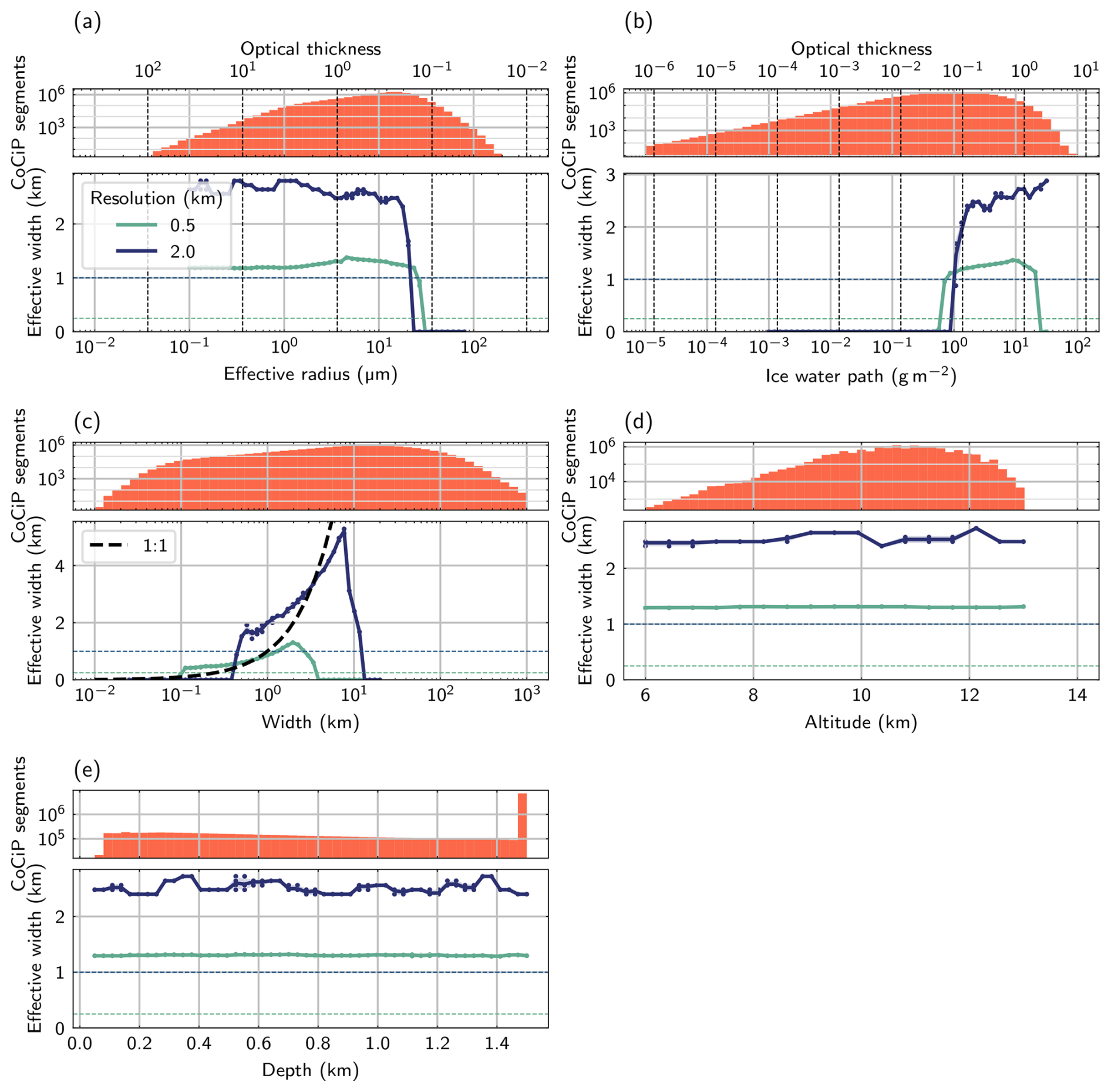
Figure 3 Tests for changes in contrail observability (i.e. observed effective width) when varying r_eff (a), IWP₀ (b), width (c), altitude (d), and depth (e) of contrails. Solid blue-green lines are the average w_eff detected over four noise realisations for two different imager resolutions, with scatter points showing the individual measurements. The corresponding dashed lines are the $w_{\text{eff}}\ge R/\mathrm{2}$ condition for detection. The response is plotted alongside histograms of global contrail properties (from CoCiP population 1). The dashed black line in panel (c) indicates equal w_eff and prescribed contrail width.

3 Contrail parameter observability tests

3.1 Single-parameter sensitivity tests

Different contrail properties (IWP₀, r_eff, width, altitude, and depth) were each varied while holding other properties constant. The impact on the detected w_eff (Eq. 4) of these parameters is shown in Fig. 3.

In each observability test, properties are varied with respect to a baseline contrail, which is 2 km wide, 0.5 km deep, and has a base altitude at 11 km, an r_eff of 10 µm, and an IWP₀ of 2 g m⁻². The baseline properties are chosen as representative of global contrail properties (based on CoCiP population 1). This analysis is intended to abstract the observability consequence of each individual contrail property from the consequence of the others, so no attempt is made to ensure that contrails simulated in the course of these observability tests are realistic, including no accounting for properties which are likely to covary (such as width and depth).

There is a low-optical-depth observability limit seen in the high-r_eff and low-IWP₀ regimes of Fig. 3a and b – as expected, contrails which are too optically thin are unobservable. Very optically thick contrails also appear undetectable, creating a high-IWP₀ limit of observability seen for the 0.5 km resolution imager in Fig. 3b. This high-IWP₀ limit occurs when the centre of a contrail becomes so optically thick as to appear opaque to the upwelling thermal radiation in both imager channels which are differenced for the brightness temperature difference signal (used for contrail detection; Sect. 2.2). The analogous limit for the coarser-resolution imager is not seen, despite the expectation that the opacity as a function of IWP is resolution-independent. The limit occurs at higher IWP₀ for the coarser-resolution imager because the effect of the peak IWP at the centre of the profile is “averaged” over the pixel, which would include some lower IWP of the profile (Eq. 1) further from the centre. For this contrail, with this particular width, the signals in the synthetic image are simply not strong enough to cause a detection.

A significant observability response occurs as contrail width is increased, shown in Fig. 3c. The narrowest contrails are not detected, with an observability onset occurring as contrail width increases to (slightly below) the imager resolution. The w_eff detected then increases from an initial approximately 1-pixel effective width, detecting the broadening contrail. Note that the measured contrail widths differ when the same contrail is imaged using imagers with different spatial resolutions. The same underlying contrail produces contrails of different pixel mask areas, so a different w_eff is inferred. This is analogous to the dependence of cloud fraction on the resolution of a binary cloud mask, found by Shenk and Salomonson (1972).

Wide contrails are also not detected. This is a limitation of the detection algorithm, which uses line kernels that highlight linearly extended regional gradients 1–4 pixels wide. The CoCiP population has a significant spread in width, including contrails with widths of up to several hundred kilometres, so this algorithm limitation would have a significant effect if untreated. Detection occurs within different upper and lower limits of width for each of the imagers tested. The high width limit is likely to be overcome if a different approach is used, given that narrower contrails with similar microphysics are detectable using this algorithm. For example, the observation could be downsampled onto a coarser grid before applying the detection algorithm. As a result, it is reasonable to consider all contrails wider than the narrowest detectable contrail with a given set of microphysical properties to be detectable.

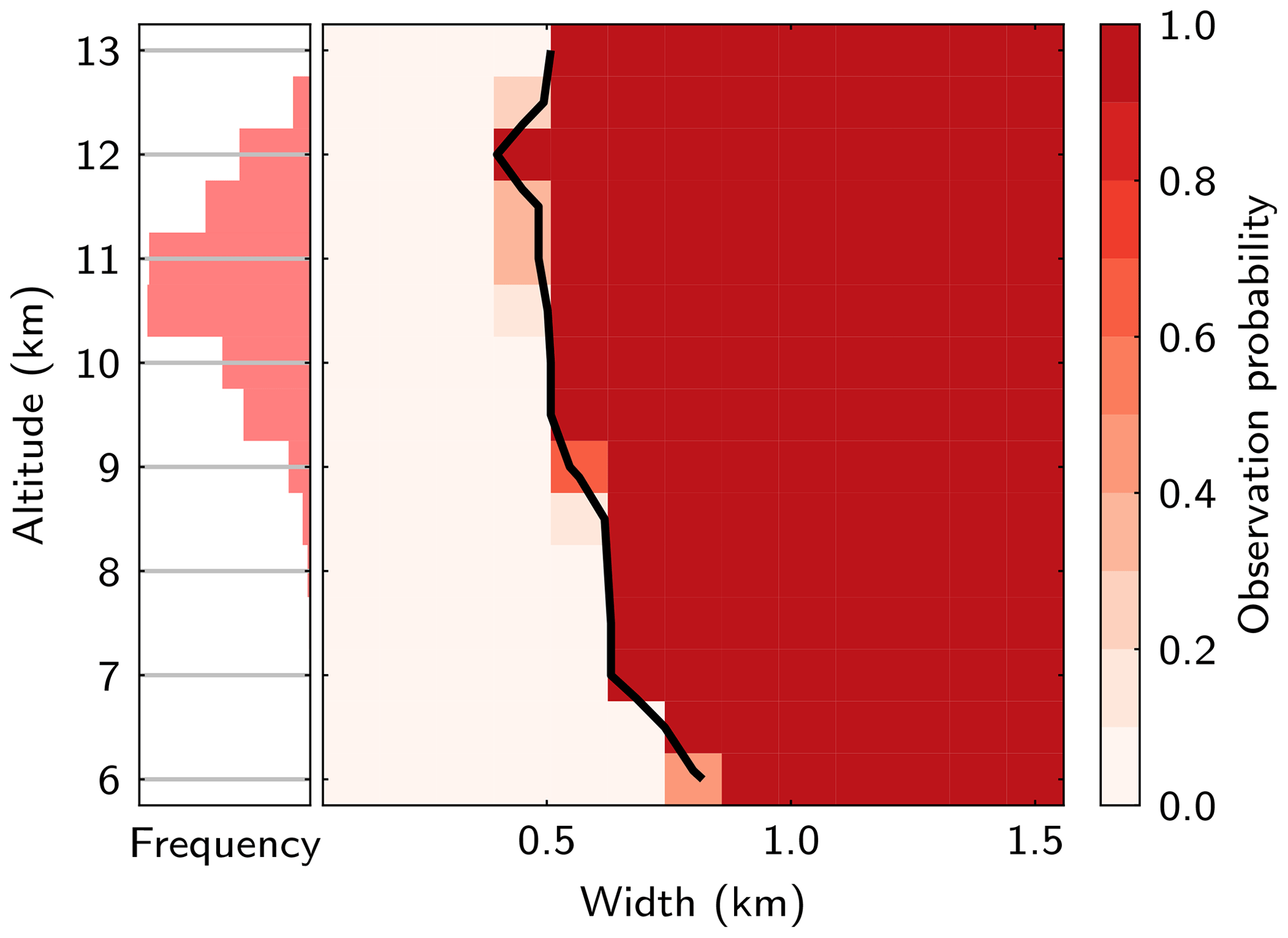
Figure 4 The observability of contrails at different altitude as width is varied, tested for a simulated 2 km resolution imager for 10 realisations of a synthetic noise field. The black contour shows the resulting observability threshold.

A contrail's altitude is expected to limit the brightness temperature contrast between the contrail and clear-sky regions of an image, limiting observability. However, contrail altitude is not found to have a significant effect on the observability of this particular baseline contrail (Fig. 3d). In fact, the altitude effect only becomes important when contrail width is less than the imager resolution, as shown in Fig. 4, where detectability has been tested at a range of altitudes for contrails with sub-grid widths. The detection probability is shown to co-vary with altitude and width, for contrails with width significantly below the imager's resolution (of 2 km). Higher contrails have greater brightness temperature contrast with the background than lower contrails, so they become observable at narrower widths (discussed in  Mannstein et al., 1999); however, this effect is small for the altitudes at which contrails form.

The vertical depth over which the contrail's IWP is spread also does not drive a strong observability response (Fig. 3e). This relaxes any observability bias that may emerge from the unrealistic distribution of contrail depths in the CoCiP histogram in Fig. 3e.

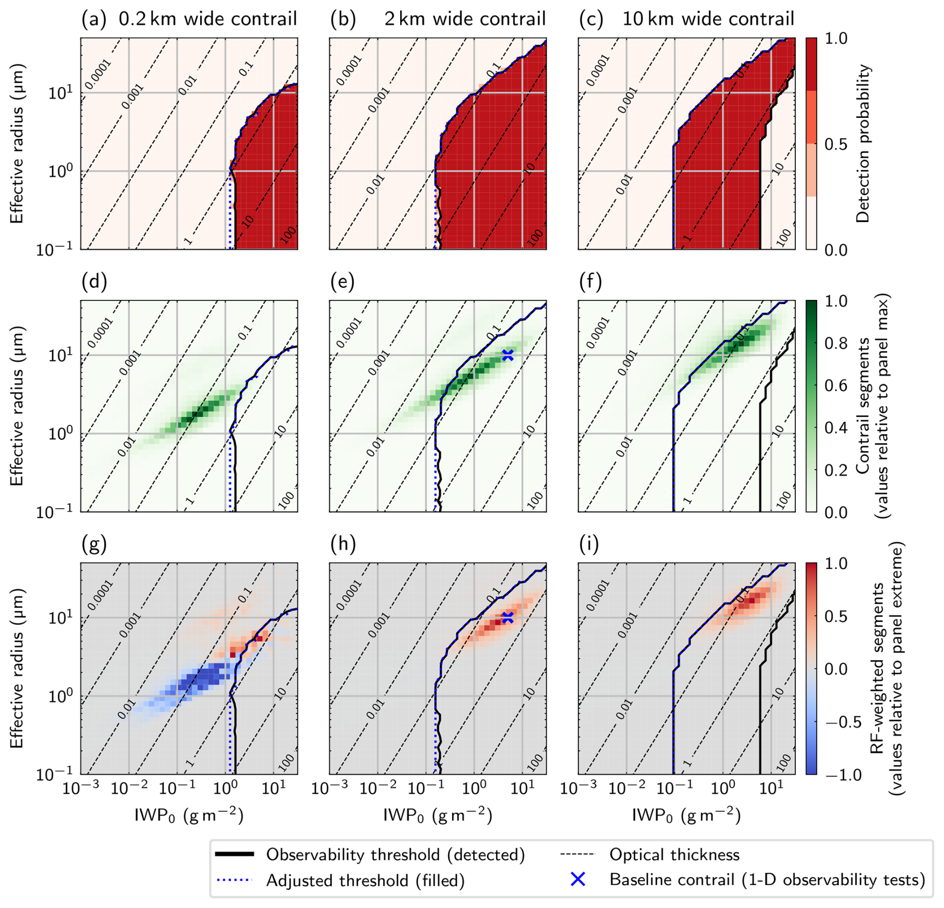
Figure 5 Illustrative slices from a contrail observability test for three contrail width bins (chosen from 30 total bins): 0.2 km (a, d, g), 2 km (b, e, h), and 10 km wide (c, f, i) contrails. The observability threshold is plotted over the derived detection probability (a–c) and histograms of CoCiP population 1 (d–f) and of the same population weighted by the mean net RF of the contrails in each bin (g–i). The histogram values (d–i) are relative to the magnitude of the extreme value in each plot. The “adjusted threshold” represents the observability threshold adapted to include all theoretically observable contrails, without the high-width algorithm deficiency. Contours of the contrail optical thickness (estimated based on IWP₀ and r_eff) are also shown.

3.2 Contrail observability threshold

The analysis of Sect. 3.1 leads to the identification of a parameter space consisting of those properties which have a strong control on contrail observability: IWP₀, r_eff, and contrail width. The observability of a contrail is tested in this parameter space by co-varying these three parameters. The population is split into logarithmically spaced bins in each dimension, including contrail width bins between 0.025 and 25 km wide, r_eff bins between 0.1 and 50 µm, and IWP₀ between 10⁻³ and ${\mathrm{10}}^{\mathrm{3}/\mathrm{2}}\mathrm{g}{\mathrm{m}}^{-\mathrm{2}}$. We neglect altitude variations because they only had a weak observability effect (Fig. 4), so an altitude of 11 km is assumed for all contrails. This altitude is approximately consistent with the modal altitude (Fig. 3d) and aligns with the aim of a maximally observable case (Fig. 4).

Detection was performed on four realisations of the synthetic radiance field for each set of contrail properties, testing the measured w_eff (Eq. 4) against the condition for detectability ($w_{\text{eff}}>R/\mathrm{2}$). A “probability of observation” p_obs is then derived (the proportion of noise realisations with a “detectable” outcome). The detectability threshold is then the surface bounding the region in the parameter space where p_obs>0.5.

Figure 5a–c shows the observability threshold derived for a GOES-ABI-like 2 km resolution imager for three different width bins in this parameter space. The chosen widths illustrate the different observability behaviour of contrails narrower than, comparable to, and wider than the imager resolution. Histograms showing the distribution of CoCiP population 1 contrail r_eff and IWP₀ are shown in Fig. 5d–i, alongside the derived threshold. The choice of parameter space and logarithmically spaced bins enables both these distributions and the threshold to be clearly resolved.

Contrails with a larger optical thickness tend to be more observable than those with a lower optical thickness, aligning well with expectations. Regardless of contrail width, contrails with optical thickness below approximately 0.05 were found to be undetectable, consistent with past work (e.g. Kärcher et al., 2009). Additionally, the detectability of more optically thick contrails is seen to depend on the specific properties – particularly the contrail width, r_eff, and IWP₀. An apparent exception to the high optical thickness observability emerges at high width, where the most optically thick contrails appear undetectable. This is an artefact of the same high width limit of detection discussed in Sect. 3.1. We adjust the threshold to make the subsequent analysis applicable to detection algorithms without this deficiency. This is achieved by treating the threshold as defining a “minimum width” given by the narrowest contrail with each r_eff and IWP₀ that is detectable. This adjusted threshold is shown using the dotted blue contour in Fig. 5.

For contrails significantly narrower than the imager's resolution, a higher contrail optical thickness is required to detect the contrail (Fig. 5a, compared to b and c). CoCiP population 1 contrails in the 0.2 km width bin (Fig. 5d) are mostly “too narrow” to be detected, as is much of their forcing (Fig. 5g) A wider contrail with the same properties would be detectable. It is notable that these contrails, which are less than 1 pixel wide, can still be observable but that no width-independent “optical thickness threshold” can be used to define observability.

The CoCiP population 1 contrails and net contrail forcing in the 10 km bin are mostly observable (Fig. 5f, i). However, there is a significant proportion of contrails and their forcing which does remain outside the adjusted threshold at these high widths. Such contrails (where there is no width in the parameter space that would make a contrail with that r_eff and IWP₀ detectable) are “too optically thin” to be detected.

3.3 Principal components of variability in the parameter space

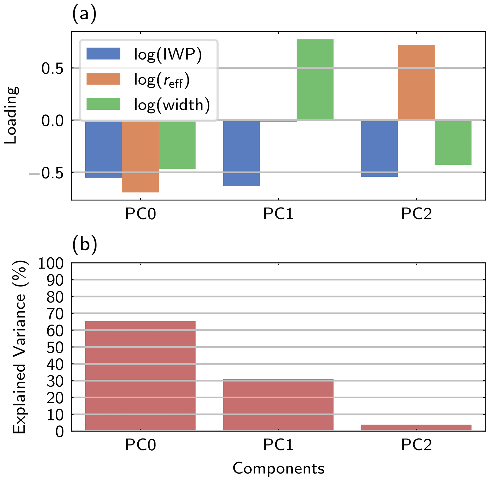
Figure 6 The principal components (PCs) of the CoCiP population in an IWP₀–r_eff–width parameter space. Panel (a) shows the PC loadings with each variable, and panel (b) shows the percentage of variance explained by variability in the direction of this PC.

Through the 1D analyses of Fig. 3, it is clear that the observability is a strong function of the three parameters used for the observability space (IWP₀, r_eff, and width). The histograms in Fig. 5d–i suggest that the CoCiP population approximates a plane in this space (on logarithmic axes). This behaviour is important to make sure the derived observability threshold is robust to any variability in the contrail properties.

Principal component (PC) analysis (Lever et al., 2017) can indicate the key directions of variability and the amount of population variability which exists in these emergent directions. Examining the PCs and their associated proportion of variance enables us to establish to what extent the population lies on a plane in this space, and the principal components offer some physical insight. Values of log (IWP₀), log (r_eff), and log (width) are standardised to have unit variance before analysis because of their different scales.

Figure 6a shows the principal components within this parameter space, and Fig. 6b shows the associated proportion of the variance. Together, PC0 and PC1 describe 96 % of the variance of the population. PC0 is a component describing IWP₀, r_eff, and width co-varying; i.e. bigger contrails tend to be more optically thick, and this is presumed to be related to the temporal growth of the contrail. PC1 comprises anti-correlated IWP₀ and width at an approximately constant effective radius – this can be interpreted as contrail segments at a different point in their evolution, with the fixed population of ice crystals being spread over a growing width as a segment ages.

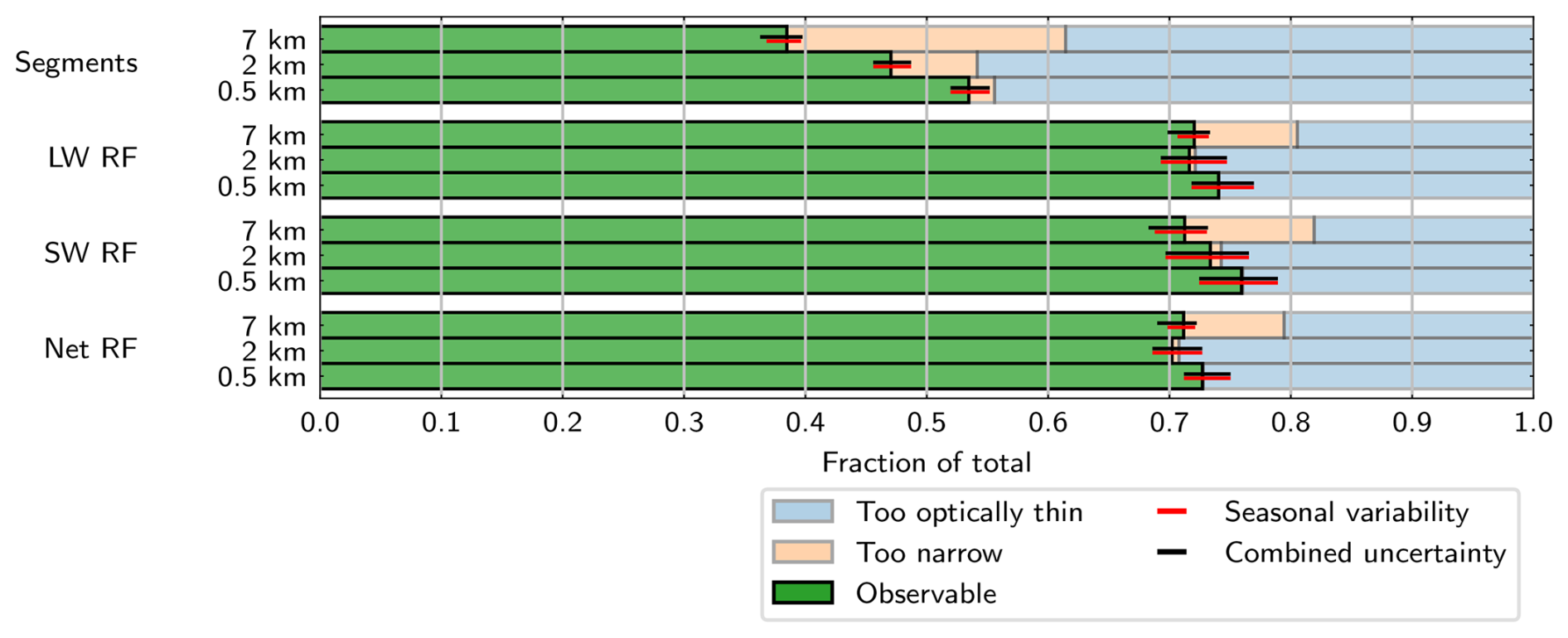
Figure 7 The fraction of contrail segments that are theoretically observable using imagers with 7, 2, and 0.5 km spatial resolution, shown as a proportion of contrail segments and weighted by their instantaneous LW, SW, and absolute net RF (per unit length) and based on the distribution of properties modelled in CoCiP population 1 using Jet-A1 fuel. Unobservable contrails are categorised as either too narrow or too optically thin to be observable. Error bars are a combination of the variability in contrail properties due to seasonal effects (also shown independently) and uncertainty in the derived threshold based on the observable proportion using 0.25 and 0.75 p_obs thresholds.

4 Population observability consequences

4.1 Contrail segment observability

4.1.1 Idealised detection efficiency estimates and uncertainty

Figure 7 shows the percentage of contrail segments which are observable using simulated 0.5, 2, and 7 km resolution imagers. The observable fractions are based on the combination of CoCiP population 1 and the observability threshold found in Sect. 3.2, including the adjustment for wide contrails. The thresholds are shown in Fig. 8a–c as the minimum width required for detection of a contrail as a function of r_eff and IWP₀. The 2 km resolution is most representative of the current generation of geostationary imagers (like GOES-ABI), so it is the focus of this discussion. The coarser resolution is chosen as a point of comparison and is achieved by previous-generation geostationary imagers at mid-latitudes (e.g. MSG-SEVIRI).

In 2 km resolution satellite images, (46±2) % of contrail segments are found to be observable; this increases only 7 percentage points when a 0.5 km imager is used. The observability gain from the higher resolution is minimal because the significant majority of unobservable contrails are too optically thin to be observed, rather than too narrow. Optically thin contrails are not as accessible via imager resolution enhancements – observations of these cases are instead limited by detection algorithm thresholds and ultimately imager noise. Similarly, the decrease in resolution from the even coarser 7 km resolution imager is relatively modest, but the proportion “too optically thin” decreases in favour of the population “too narrow” to be detected. This is a result of the specific detection algorithm applied: the coarser images are better suited for detecting theoretical very wide contrails, so the upper limit on contrail width that is theoretically detectable is relaxed, and the detectability threshold can be defined in some more optically thin bins.

Detectable contrails contribute (70±2) % of the net radiative forcing in simulated 2 km resolution images (Fig. 7). The detectability of forcing is higher than the detectability of contrail segments, meaning that the contrails with stronger radiative forcing are a more observable population than the population as a whole. This aligns with expectations: a small percentage of strongly forcing contrails contributes most of the net warming (Teoh et al., 2022a), and more optically thick contrails tend to warm strongly (Meerkötter et al., 1999). This interpretation is also consistent with the findings that the observable fraction of contrail forcing does not vary significantly with imager resolution or by component of forcing (because the few optically thick contrail segments causing much of the forcing are sufficiently wide that the resolution dependence is less significant).

The uncertainties given are a combination of a p_obs-derived threshold uncertainty and seasonal variability. The p_obs uncertainty describes variations in the observability threshold and is derived based on the different realisations of the imager noise field. The range is based on the proportion observable if the threshold is defined based on p_obs>0.25 and p_obs>0.75 conditions (i.e. detectable or undetectable in only one of the four realisations of the synthetic image). The impact of seasonal variability is assessed by taking the standard deviation of the observable fraction obtained when subsetting CoCiP population 1 based on the month of the year. Both the combination of the two uncertainties and the uncertainty due to variability are shown in Fig. 7, and the variability in contrail properties clearly dominates the component due to instrument noise in this idealised case.

4.1.2 Speculative relaxation of limits imposed by the detection algorithm

The contrail observability is dependent on the contrail detection algorithm used. The observability threshold (derived in Sect. 3.2) is based on the lowest width for which a set of optical-thickness-driving microphysical properties (i.e. r_eff and IWP₀) produces simulated brightness temperature field in which the contrail is detected using the detection algorithm introduced in Sect. 2.2. The algorithm used contains thresholds tuned on human-labelled datasets to optimise precision and recall, as distributed in McCloskey et al. (2021). Real contrails which were not identified by the human labellers would be spuriously considered “false positives” if picked up by the detection algorithm. This means that the algorithm reflects the contrails theoretically observable by the human labellers. Mannstein et al. (1999) chose a brightness temperature difference threshold uniquely low compared to existing algorithms at the time (0.2 K) and much lower than the threshold in the tuned algorithm (1.33 K), aiming to use the contrail's geometry rather than thresholding to ensure reliability.

As a test, a less conservative detection algorithm was constructed by reducing applied thresholds from the human-labelled tuned values to the least conservative between these and the values used by Mannstein et al. (1999). It should be noted that such an algorithm poses an increased risk of false positive detection, so it may only be practically applied when this risk can be reduced (such as the targeted observation of a contrail known to exist or suspected to exist in a time step following one where it is more confidently detectable). The algorithm of Mannstein et al. (1999) was designed for use with a different imager, so such algorithm adjustments need testing for their specific application. When applied to 10 000 realisations of the clear-sky instrument noise field (i.e. synthetic image with no contrail), no false positive detections occurred using this new algorithm, indicating that it is suitable to speculate on potential achievable detectabilities, albeit in this very controlled case. The threshold derived using this less conservative algorithm is shown with an evolving contrail in Fig. 8d. In this case, using the same high-width adjustment of Sect. 3.2, (89±1) % of segments and more than 99 % of all components of forcing are theoretically observable in fields simulated with 2 km resolution.

Observation-independent ground truth data do not exist, so these detectabilities are unachievable for general observation (because false positives cannot be controlled for). However, this initial analysis suggests that the observability limit derived here can be relaxed if the risk of false positives can be mitigated, for example, in the case of targeted observation of specific contrails based on advected flight tracks, where a likely location of the contrail is known.

4.1.3 Significant limitations imposed by more-complex backgrounds

To illustrate the significant impact caused by background cloud and demonstrate that this is a maximum accessible fraction of contrails, the observability of contrails is tested against a layer of background cirrus. Additional radiative transfer simulations are made for this case. The background cirrus layer is 500 m deep, at 8 km altitude, with an effective radius of 5 µm (chosen as the intersection of the two ice cloud parameterisations due technical limitations) and an IWP of 25 g m⁻². The layer has an optical thickness of approximately 3.

The cirrus layer significantly reduces the brightness temperature contrast between the contrail and the background, decreasing contrail detectability. Detectability is tested using the same detection algorithm thresholds based on human-labelled datasets described in Sect. 2.2. Under this analysis, less than 2 % of contrail segments in CoCiP population 1 and less than 3 % of each component of forcing were detectable. The derived minimum width threshold for observability is illustrated in Fig. 8e. Only the most optically thick contrails were detectable. The minimum width required for detection shows a discontinuity at high IWP₀, similar to the limit in Fig. 3b. In this case, the combination of background cirrus and contrail causes does not cause a brightness temperature difference signal at the centre of the contrail, as it is sufficiently optically thick to be opaque in both the channels that are differenced. The high IWP₀ discontinuity in the threshold does not completely prevent detection but significantly increases the minimum detectable width. This is because the IWP profile (Eq. 1) varies gradually enough in wide contrails that their edges remain detectable.

The chosen effective radius (due to technical limitations) would be relatively unphysical for a mid-latitude natural cirrus layer (although it may represent, for example, observation against a contrail cirrus outbreak). To provide a comparison, a similar test against a 30 µm cirrus layer is also performed for contrails whose r_eff is high enough that radiative transfer simulations can be made. The IWP is also increased to maintain an optical thickness of approximately 3. The derived threshold is shown in Fig. 8f. Against this background, contrails with a higher effective radius become observable, demonstrating that this cirrus layer would pose less of an obstacle to contrail detection. From the data available for contrails below 10 µm, the two background cirrus thresholds appear comparable at lower effective radii.

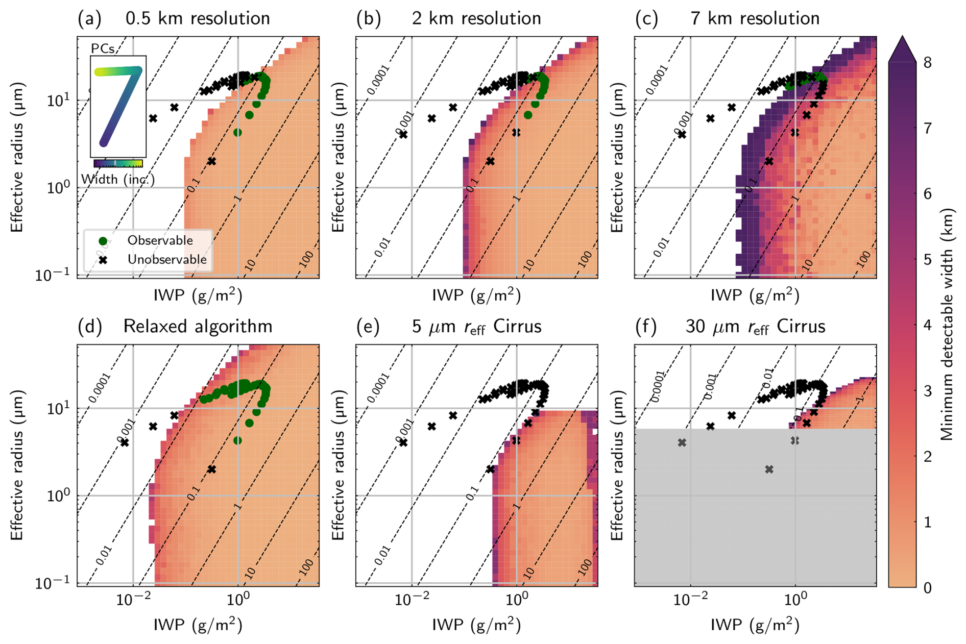
Figure 8 Representative trajectories of a contrail's evolution in parameter space against the derived minimum width thresholds for detectability found in the course of this work. The IWP₀ and r_eff of a single contrail's evolution at each model time step are marked with the following different thresholds: using the original algorithm at 0.5 km (a), 2 km (b), and 7 km (c) spatial resolution images; with the less conservative thresholds discussed in Sect. 4.1.2 (d); and against layers of background cirrus with 5 and 30 µm effective radii (e, f). The same 2 km resolution imager of panel (b) is used for panels (d–f). Omitted effective radii in the case of 30 µm cirrus are due to technical limitations of the radiative transfer infrastructure. Also included (on inset axes in panel a) are the principal components identified in Sect. 3.3, coloured by their evolving width, which broadly correspond to the stages of contrail evolution.

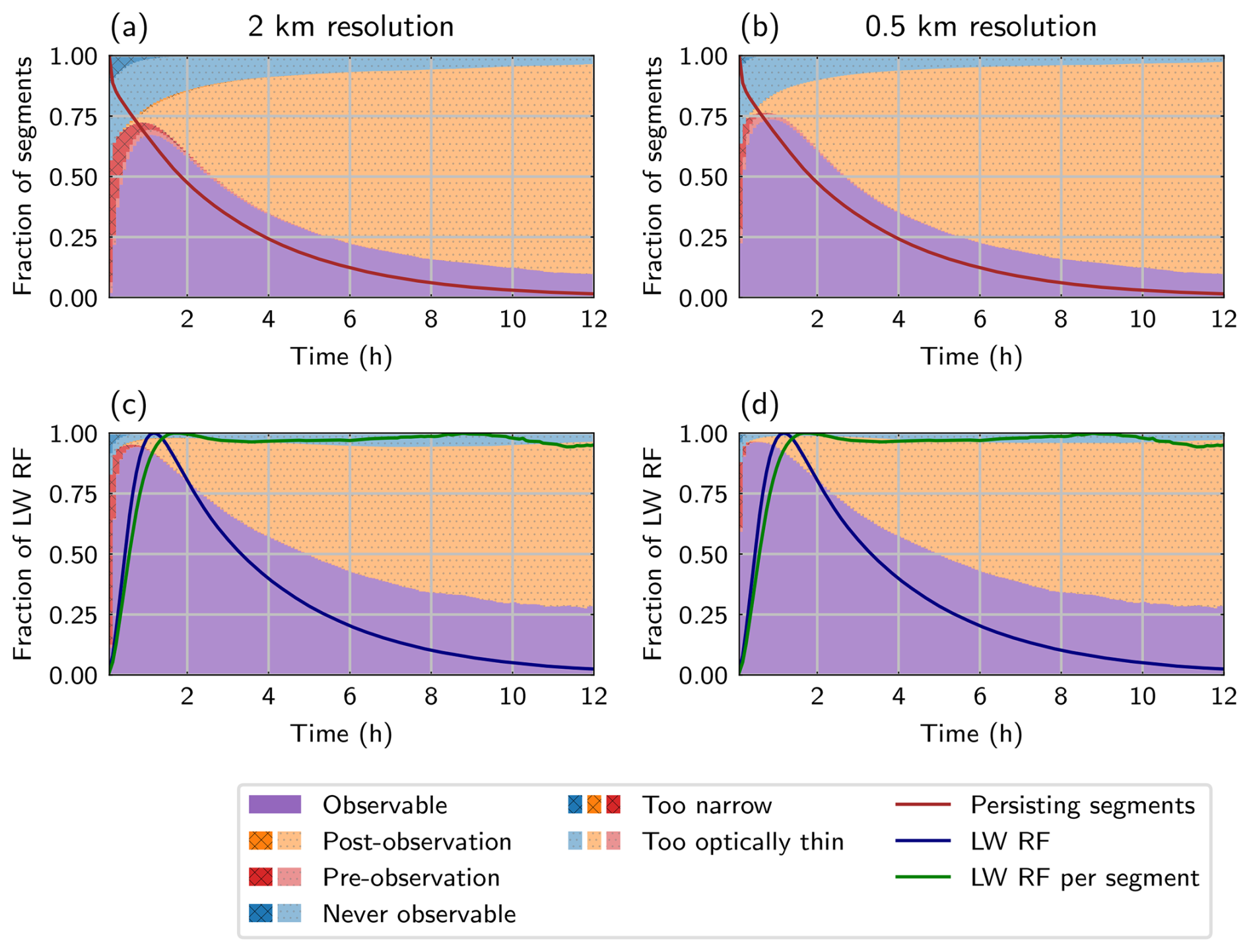
Figure 9 The time evolution of observability: the observability status of contrail segments (a, b) and their proportions of forcing (c, d) formed globally within the time-evolving sample, using Jet-A1 fuel, for both 2 km (a, c) and 0.5 km (b, d) imagers. Using the adjusted observability threshold of Sect. 3.2 (Figs. 5, 8a), segments are categorised as “observable”, “never observable”, “pre-observation” (have not yet been observable but will be observable later), or “post-observation” (were observable earlier in their evolution but are not at this age). Unobservable contrails are also categorised as either too narrow or too optically thin to be observed. Lines indicate the number of persisting contrail segments (a, b), LW forcing (c, d), and the per-segment mean LW forcing (c, d) due to contrails of a given age (relative to other CoCiP population 2 age bins).

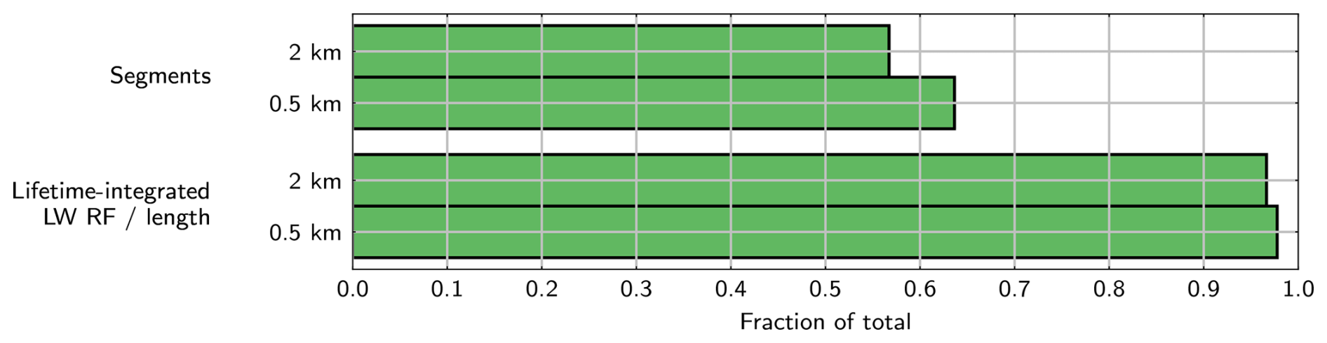
Figure 10 The proportion of CoCiP population 2 contrails (and contrail $\text{EF}/\text{length}$) observable for at least one model time step, as determined using the contrail detection algorithm threshold tuned on hand-labelled data (the algorithm as distributed in McCloskey et al., 2021).

4.2 Observability with contrail ageing

A contrail's properties evolve as it ages, so observability also has characteristic evolution. The evolution of one contrail from CoCiP population 2 is shown against the different observability thresholds of this work in Fig. 8. This behaviour is typical of a contrail's time-evolving properties. The stages of the contrail's evolution (growth, persistence, and dissipation) broadly align with the two PCs identified to explain a large proportion of the variance in CoCiP population 1 (Sect. 3.3). The observability status of the contrail is marked – at formation, it is initially too narrow to be observed, but, as it grows, the minimum observable width threshold is crossed and the contrail becomes observable (except when imaged against background cirrus; Fig. 8e, f). During the persistence phase, the contrail spreads over a wider area, decreasing IWP₀ at approximately constant r_eff. During this time, this contrail becomes unobservable due to being too optically thin. Finally, this contrail dissipates, with ice crystals eventually decreasing in size, until it is removed from the model population at its “end of life”.

Figure 9 shows the proportion of contrail segments with different ages that are observable in CoCiP population 2 along with the proportion of LW forcing. Each contrail segment is tracked for its entire CoCiP persistence lifetime (which is capped at 12 h), and observability is assessed at each time step. Data are binned based on model time steps since formation; that is, contrails in the first bin are formed between 0 and 5 min ago and survive until the time at which the model outputs data. This means that some contrails with a persistence lifetime of less than 5 min are never represented in the analysis, similarly to the population of contrails captured in regular satellite observations. LW forcing is used because its positive definite nature simplifies calculations and reduces variability in forcing estimates due to solar zenith angle (meaning the results are instead focused on the link between contrail properties and radiative importance). A small number of contrail segments are temporarily unobservable after their period of observation; these are classified as “post-observation”, and this affects 8 % of segments in the 2 km imager and 7 % in the 0.5 km imager.

Each of the panels in Fig. 9 is overplotted with the relative contribution of contrails with a given age to the instantaneous population of contrails. Specifically, the proportions of contrail segments are shown alongside the fraction of persisting segments, equivalent to the fraction of segments that would be expected to be a given age for a given time. The proportions of forcing are shown with the contribution of contrails with a given age to the instantaneous global forcing due to contrails (along with the per-segment mean forcing of contrails with a given age, approximately equivalent to the relative forcing per unit length of contrails with a given age).

The population of contrail segments decays with the dissipation of contrails (with a characteristic e-folding lifetime of around 3 h). Note that the forcing per segment peaks just less than 2 h after formation, remaining at this value for the remainder of the persistence, as an increasingly optically thin contrail spreads over a broadening width. The total LW forcing decays much like the number of persisting segments, as some contrails dissipate.

The population of never-observable contrails consists of both contrails that are both too narrow and too optically thin. This population is much reduced in the forcing-weighted analyses (Fig. 9c, d), suggesting that keeping track of these contrails is less important for monitoring the radiative forcing. However, it is apparent that the formation (or lack) of a significant proportion of contrail segments would not be able to be validated using satellite-borne imagers.

Pre-observable contrails tend to be too narrow to be observed, becoming observable when they have broadened sufficiently. A pre-observable population persists into the forcing-weighted case, but the high-resolution imager provides a significant improvement in accessing this population.

When the contrails are no longer observable, they are overwhelmingly more likely to be too optically thin than too narrow. It is at this stage that contrail observability appears to decouple from the contrail lifetime – the post-observable phase does not seem to be a transient phase as the contrail dissipates but a growing proportion of the contrails. Again, it should be noted that the number of contrails and total forcing are increasingly small with ageing, so this increasing fraction remains relatively small as a fraction of the instantaneous population.

As a check for consistency with the analysis in Fig. 7, the detection efficiencies of CoCiP population 2 contrails and of their RF are estimated. This is performed by integrating the product of the observable proportion of contrails (or of LW RF) with the persisting fraction of segments (or relative contribution to the total LW RF) over the time since contrail formation. Approximately 45 % of contrail segments are found to be theoretically observable with the 2 km imager, increasing to 50 % for the 0.5 km resolution imager; 69 % and 70 % of LW forcing is theoretically observable for the 2 km and 0.5 km resolutions, respectively. Comparing to the variability ranges derived based on CoCiP population 1 (Fig. 7), these values are mostly within the ranges of uncertainty, with the exception being the forcing observability with a 0.5 km resolution (which lies only slightly below). This variability highlights that the day-to-day variability in contrail properties and estimated forcing is even more extreme than seasonal variability.

The number of CoCiP population 2 contrails observed at least at some point during their life cycle is plotted for both the model population of segments and the lifetime-integrated LW forcing per unit length in Fig. 10. Around 57 % of contrail segments are observable in 2 km resolution images for at least one model time step during their evolution. This increases to 64 % with the 0.5 km resolution imager. When weighted by their lifetime-integrated LW energy forcing, this is increased to 97 % and 98 % for the 2 and 0.5 km resolution fields, respectively. Uncertainty in these values is expected to be dominated by seasonal variability (as in Fig. 7) and is not calculated for CoCiP population 2 because it is limited to a single date.

Finally, the distribution of the time between a contrail's formation and the time at which it first becomes observable is examined. This transition is highly skewed, so the median age of first observability is given, with the first and third quartiles to give an impression of the variability. In 2 km resolution images, the median time for the onset of detectability occurs at 21 min, with the first and third quartiles at 10 and 94 min. The onset occurs at a median 9 min after formation in hypothetical 0.5 km images (between 5 and 70 min quartiles). This is in good agreement with the delays to the onset of GOES-ABI (ca. 2 km resolution) observation reported by Chevallier et al. (2023) and Gryspeerdt et al. (2024), although these studies do not capture the higher limits estimated here. This is likely due to the increased difficulty in matching observed contrails to generating flights when the delay to observation increases.

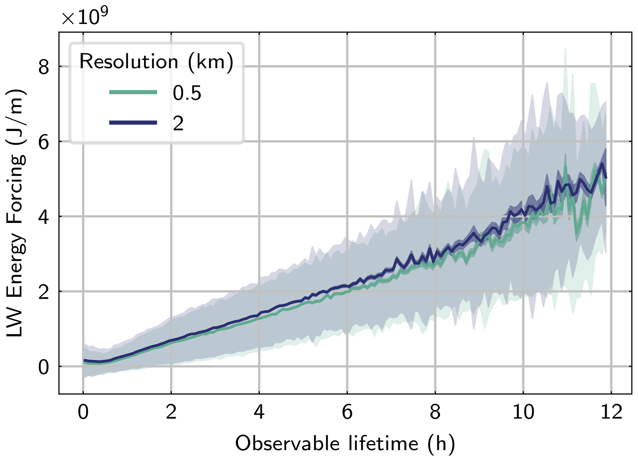
Figure 11 The relationship between lifetime-integrated energy forcing per unit length and the observable lifetime. The strongly shaded region denotes uncertainty in the mean, and the lightly shaded region is the variability (the standard deviation for contrails with a given observable lifetime).

4.3 Observable lifetime as a proxy for radiative importance

Radiative forcing during the part of the lifetime for which a contrail is unobservable may be significant. A fraction of contrails have been found both before and after their period of observability, including when weighted by their forcing (Fig. 9). Comparisons of relative radiative importance drawn from observed contrail lifetime (such as in Gryspeerdt et al., 2024) therefore carry an implicit assumption that the factors influencing the period of observability also determine the persistence lifetime of the contrail. This assumption is threatened by the “too optically thin” contrails found here, which have been shown to comprise a significant proportion of the aged contrail population. Previous contrail-tracking studies have inferred contrail lifetime from observed lifetime, requiring assumptions about initial contrail spreading rates and the generalisation of observation-derived survival functions to unobserved parts of a contrail's lifetime (Gierens and Vázquez-Navarro, 2018). The length of time for which a contrail appears in consecutive geostationary satellite images – the “observable lifetime” of the contrail – is measurable and may be a good proxy for lifetime radiative impact. We now examine the relationship between this observable lifetime and its lifetime radiative impact.

Figure 11 shows the lifetime-integrated LW energy forcing per unit contrail length as a function of the theoretically observable lifetime for the contrails in the time-evolving sample. LW energy forcing is used (as in Sect. 4.2) rather than net forcing so that net forcing variability due to the variations in SW forcing with time of day does not overwhelm the variability estimates. For both current imagers and theoretical higher-resolution imagers there is a positive correlation, with an approximately linear relationship between the observable lifetime and the LW radiative forcing for contrails observable for longer than 1 h.

There is significant variability in each observable lifetime bin, but a resolution dependence is well resolved. Observed contrails tend to have higher lifetime forcing in more coarsely resolved images. This follows from the ability of the 2 km resolution imager to only observe larger and more optically thick contrails, which in turn have stronger forcing.

Figure 12 The theoretically observable fraction of contrail segments and instantaneous radiative forcing (as in Fig. 7), based on CoCiP population 1, assuming fractional adoption of SAF biofuel leads to reduced effective emission of ice. A 2 km spatial resolution imager is used.

4.4 Observability with the adoption of alternative fuels

Figure 12 shows the potential observability consequences of decreased emission of activating particulates – assumed to be dominated by soot, as is the case for current fuels. The observability of a contrail population formed during fractional adoption of alternative fuels has been determined. The population results from CoCiP, run with identical flights and meteorology, but assuming a fractional adoption of SAF in the fuel in all aircraft (rather than Jet-A1 fuel) results in decreased ice emission indices. The modelling methodology follows that of the SAF experiments of Teoh et al. (2022b), using the 30 %, 50 %, and 100 % SAF adoption experiments, which have been expanded to the global flight inventory of Teoh et al. (2024a).

There is a significant decrease in the observable fraction of contrail segments and forcing. In a less soot-rich environment, fewer contrail ice crystals are expected to form, so they grow larger (Voigt et al., 2021). A shift in the populations of Fig. 5 towards higher effective radius (and lower optical thickness) moves the contrails nearer the observability threshold, corresponding to these drops in observability. In simulated 2 km images after 100 % adoption, only (25±3) % of segments are observable and only (47±4) % of net forcing is theoretically observable. This means that coverage estimates for contrails produced by aircraft generating fewer non-volatile particulates will be based on fewer observations, making them (and potential assessments of radiative impact) more uncertain. The estimated uncertainty in detection efficiency is again dominated by seasonal variability (as in Fig. 7).

Teoh et al. (2022b) explore the derived climate benefit of SAF adoption. It should be noted that, while a lower fraction of contrails is observable, there are also fewer contrail segments in the CoCiP population and a reduced net contrail forcing. The activation of volatile particulates in less soot-rich exhaust (Ponsonby et al., 2024) has not been considered for this model population. Volatile activation would act to partially counteract the changes in observability driving the decreased observable fraction found here.

5 Discussion

5.1 Applicability of methodology

This analysis is limited to the very simple case of straight-line contrails against a plain ocean background, with obstacles to observation from imager properties and the thresholds from the algorithm applied. The algorithm, trained on hand-labelled contrails, provides insight into the contrails practically accessible in real satellite images. These are more restricted than the absolute limits of detection in the artificial radiance fields (which would only be imposed by imager resolution and noise) but are a good reflection of the best case possible when applied to real observations because the algorithm restrictions reflect the limits of certainty against false positive detections.

The minimally realistic synthetic contrails modelled here are intended as a maximally detectable test case. This approach is designed to establish whether some contrails go undetected with current instruments even in the most straightforward case. The approach also treats contrails as extended objects – testing not only that contrails produce a signal but that the extended signal is detectable as a contrail, aligning with detection methods that take the spatial properties of the contrail into account. The brightness temperature contrast, and particularly background inhomogeneity, has previously been noted to limit the detection efficiency (Mannstein et al., 1999). Contrails imaged over land or against background cloud should be expected to be less observable than is established using this analysis because this will introduce additional features with reduced contrast to the brightness temperature fields used for detection, owing to their colder temperatures (particularly for underlying cloud) or reduced emissivity (particularly for surface features). A demonstration of the overwhelming impact background can have was made in Sect. 4.1.3, where an idealised cirrus layer obscured the detection of nearly all contrails. Conversely, observability may be increased when targeted observation of a contrail known to exist is possible (where a less conservative detection algorithm could be applied, as discussed in Sect. 4.1.2). This is well illustrated by the work of Vazquez-Navarro et al. (2010) and Vázquez-Navarro et al. (2015), demonstrating that contrails detected using a higher-resolution non-geostationary imager enabled targeted observation in coarser-resolution geostationary observations for contrail evolution to be tracked. This tracking method also stands to enable the consideration of detected contrails beyond their initial linear phase.

Additional factors influencing contrail observability are likely to include contrail latitude and viewing zenith angle more generally, which would affect the dimensions of the imaged grid and optical paths for radiative transfer (Maddux et al., 2010). These variations within regions of the same satellite field of view are not considered, to simplify the parameter space and the analysis of unobservability causes. This also aligns the approach with the best-case observability. The analysis in this work is restricted also to a single atmospheric profile and background (including surface temperature and emissivity). More physical atmospheric profiles would also impact brightness temperature contrast slightly, but this smaller effect is not treated here, again decreasing complexity and allowing more direct consideration of the cause of detection limits. Additionally, the use of 1D radiative transfer simulations neglects 3D effects (Cornet et al., 2010).

Uncertainty in the derived threshold relative to instrument noise has been found to be small relative to seasonal variations in the properties of CoCiP population 1 and their estimated radiative forcing. This highlights the importance of considering changes to contrail observability due to their actual background. The variability in observability has been found as a result of the changing contrail properties alone, not the varying meteorology. It is clear that meteorology will play a further role in enhancing variability in detection efficiency, based on the adjusted threshold of Fig. 8c in the presence of background cirrus. Unconsidered uncertainties include inaccuracies in the CoCiP-derived population and contrail properties.

5.2 Relevance to applications of contrail observation

The fact that some contrails remain unobservable in these tests demonstrates that detectability is a relevant consideration for observational applications, such as the observation of contrail radiative forcing. Fig. 7 indicates that at least (30±2) % of net contrail forcing goes unobserved using current 2 km resolution geostationary imagers, and Fig. 5 shows that there is a microphysics dependence beyond a simple optical thickness threshold for observability. This is due to a combination of contrails whose observation is optical thickness and resolution limited, of which only the contrails that are too narrow are accessible in theoretical higher-resolution images. As seen in Fig. 9d as compared to Fig. 9c, this corresponds to the observation of contrails earlier in their evolution, should resolution be improved. Particular care is needed to compare contrail coverage when there is a change to contrail microphysics (such as in the adoption of biofuels; Fig. 11) where a change in observability may have been induced. Further caution is needed when comparing masked contrail grids on images with different resolution – in Fig. 3, different effective width values are measured when using different spatial resolutions.

One may seek to determine the efficacy with which contrail formation has been mitigated, for example, in a trial attempting to avoid forming contrails (Molloy et al., 2022). For this, effective flight matching as well as efficient detection is required, as described in Geraedts et al. (2024). It has been shown that the majority of instantaneous forcing is theoretically observable using current instruments (Fig. 5), when tested in the ideal case shown here. Furthermore, in Sect. 4.2, 97 % of lifetime-forcing weighted contrail segments are shown to be observable at least for some time in their evolution. This provides reassurance that most of the most climate-relevant contrails are observable at some time during their life cycle. Effective flight matching relies on the detection of contrails shortly after their formation to minimise any errors that develop between advected flight path and detected contrail. Here a higher-resolution contrail detection technique would make a significant difference – most contrails are detectable within 9 min of their formation (Sect. 4.2), compared to 21 min for the 2 km imager.

A final application in need of improved contrail observation is the validation of contrail models, a need laid out by Schumann et al. (2017) and Kärcher (2018). The thresholds derived here form a foundation to consider which contrails are observable and how many may need to be observed to draw confident conclusions about the predictive power of the models. These validation tasks often then require retrieval of the contrail cirrus properties and variability beyond just the simple detection of contrail coverage. Care is required in applying instruments to this task, illustrated by the varying effective widths measured for the same contrail imaged at different resolutions, Figs. 2 and 3.

6 Conclusions

Infrared imagers carried by geostationary satellites are well-placed to make widespread observations of the time-evolving properties of contrails. The detection of contrails is limited both early and late in their evolution: imaged radiance fields are coarsely resolved with respect to the geometry of young contrails, and aged contrails are wide and disperse. This work highlights the contrails that should not be expected to appear in images from geostationary satellites, even in the most ideal conditions, as a function of contrail properties and detection methods.

Satellite contrail observations were simulated for simple straight-line contrails with a Gaussian profile, against a plain background, laid out in Fig. 1. A Mannstein et al. (1999) style line filtering algorithm was used to test the observability of contrails in these simulated radiance fields (Fig. 2) modelled with different properties. Firstly, contrail width, IWP₀, r_eff, depth, and altitude were varied independently (Fig. 3). Altitude was not seen to be a major driver of unobservability, particularly at altitudes where contrails exist (Fig. 4). Then, an “observability threshold” was found by co-varying the properties which produced strong observability responses (IWP₀, r_eff, and contrail width). The threshold was applied to the distribution of these properties given by a model-derived population of contrails (CoCiP population 1 of Sect. 2.3) and to their estimated forcing. The outcome of this observability test for contrails with three different widths is shown in Fig. 5.

The detection efficiencies of contrail segments and their forcing was derived, based on this sample of contrails distributed in time of day and year (Fig. 7). The most radiatively important contrails are more likely to be theoretically observable than the population as a whole. The unobservable fraction of the instantaneous global population of contrails varies from (62±2) % (of contrail segments in 7 km resolution images) to only (35±3) % (of SW forcing in 0.5 km images). The observability is strongly sensitive to the background – a simple layer of background cirrus shifts the observability threshold to include only the most optically thick contrails (Fig. 8c), obscuring detection of almost all contrails in the population.

The threshold was also applied to the time-evolving properties of contrails (Fig. 8). By analysing contrail segments forming globally over a 24 h period (CoCiP population 2 of Sect. 2.3), the evolving observability behaviour (Fig. 9) was derived. Most contrails are theoretically observable at least at some point in their evolution. Around 57 % are visible in current 2 km resolution imagers, comprising 97 % of the total radiative forcing from the contrail population (Fig. 10).

It was shown that the average lifetime energy forcing is a strong function of the observable lifetime for the contrail population forecast by CoCiP (Fig. 11). This relationship enables comparisons of the radiative importance to be drawn from the length of time for which a contrail is observed. Factors not considered here may obscure this result, particularly the development of a contrail outbreak or other meteorological evolution.

Finally, the limitations of these satellite observations are found to be increasingly important when assessing the efficacy of climate change mitigation strategies. It was shown that widespread adoption of cleaner-burning fuels would lead to a significant drop in contrail observability. A 20 percentage-point drop in the detection efficiency of net instantaneous contrail radiative forcing is expected under a modelled decrease in ice crystal number with the theoretical complete adoption of SAF (Fig. 12). This could lead to an overstatement of the benefit of the climate action if this is not considered (if detected contrails are treated as the only contrails). Even if controlled for, extrapolation of the total impact would then be based on a smaller observable fraction. Contrail observability should be considered when assessing any action on emissions or contrail mitigation.

This work stands to be expanded to consider meteorological conditions – particularly contrail overlap with underlying cloud and contrail outbreaks – as an obstacle to observability. Observation away from the sub-satellite region has also been neglected. The impact of this effect is not straightforward. A higher viewing zenith angle reduces the effective resolution, reducing contrail observability assuming the same contrail properties and meteorology. However, the longer atmospheric path length will enhance the effective cloud optical depth, making thinner contrails easier to detect (Maddux et al., 2010). Other aspects of the observing system, such as the time of day observations are made, may bias the population of contrails which is observed. Additionally, more physical cases may impact the brightness temperature fields observed. Granularity in aircraft and engine properties stands to be considered, beyond the simple fuel case examined here.

Nonetheless, this work should lend confidence to the use of contrail observations using satellites – under best-case conditions, the most radiatively important contrails are strongly observable.