Testing ground-based observations of wave activity in the (lower and upper) atmosphere as possible (complementary) indicators of streamer events

For a better understanding of atmospheric dynamics, it is very important to know the general conditions (dynamics and chemistry) of the atmosphere. Planetary waves (PWs) are global-scale waves, which are well-known as main drivers of the large-scale weather patterns in mid-latitudes on timescales from several days up to weeks in the troposphere. When PWs break, they often cut pressure cells off the jet stream. A specific example is so-called streamer events, which occur predominantly in the lower stratosphere at mid-latitudes and high latitudes. For streamer events, we check whether there are any changes in gravity wave (GW) or infrasound characteristics related to these events in ionospheric and surface measurements (continuous Doppler soundings, two arrays of microbarometers) in the Czech Republic.

Phenomena in infrasound arrival parameters undoubtedly related to streamer events were not identified in observations of two stations located in Central Europe. Simulations of infrasound propagation show influences of the streamer events on the waveguide formed near the tropopause. Microbarom propagation is influenced by the tropopause waveguide in a limited azimuth sector and at limited distances. Due to the typical occurrence of the streamer events over the North Atlantic, infrasound stations in western Europe can be of particular interest for future studies of streamer event signatures in infrasound arrivals. Arrivals to Central Europe are through the waveguide formed between the ground and the upper stratosphere. The upper-stratosphere waveguide is not influenced by the streamer events.

Supplementary ground-based measurements of GW using the WBCI array in the troposphere showed that GW propagation azimuths were more random during streamer and streamer-like events compared to those observed during calm conditions. GW propagation characteristics observed in the ionosphere by continuous Doppler soundings during streamer events did not differ from those expected for the given time period.

1 Introduction

For a better comprehension of climate change, how well we understand the climate system in general, and the dynamics of the atmosphere in particular, is fundamentally important. The dynamical processes in the atmosphere relevant in this context take place over a comparatively wide range of scales in space and time. They include in particular both planetary and gravity waves. Planetary waves are one of the main drivers of extratropical circulation. When they break, they lead to an irreversible exchange of air masses between the equatorial and polar region due to an amplification of their amplitudes (e.g. McIntyre and Palmer, 1983; Polvani and Plumb, 1992). In the lower stratosphere, ozone can be used as a tracer for these large-scale motions, as it has a comparatively long lifetime. When planetary waves break, tropical air masses of low ozone concentration are mixed poleward into the surrounding high-latitude atmosphere (e.g. Leovy et al., 1985).

The term “streamer” lacks a precise definition, as noted by Krüger et al. (2005). They discuss various aspects of streamers, including their impact on mixing and the divergent definitions associated with them. Offermann et al. (1999) describe streamers as large-scale tongue-like structures formed by the meridional deflection of air masses. Streamers are characterized by irreversible mixing of air masses between equatorial and polar regions, which is why they might be linked to planetary wave breaking (Waugh, 1993). Eyring et al. (2003) give a climatology of the seasonal and geographical distribution of streamer events. They show that streamers often occur over the North Atlantic and can be identified by either high NO₂ or low ozone concentrations. This is why we identify streamers using total ozone column measurements in this paper. Eyring et al. (2003) show that streamer events occur most often during winter and the least during July and August in the Northern Hemisphere. During a streamer event, the wind field changes rather strongly over a comparatively small distance. Since a streamer event shows a strong wind shear at its flanks, it is expected that it excites GW (e.g. Kramer et al., 2015, 2016; Peters et al., 2003).

It is well-known that enhanced wind gradients or anticyclones can lead to the excitation of gravity waves (GWs) in the atmosphere (e.g. Pramitha et al., 2015; Huang et al., 2010; Kramer et al., 2015, 2016; Gerlach et al., 2003). GWs have typical vertical wavelengths from a few hundred metres to several kilometres (Wüst and Bittner, 2006) and horizontal wavelengths greater than tens of kilometres (Wüst et al., 2018; Rauthe et al., 2006); their wind fluctuations in the upper troposphere–lower stratosphere typically have maximum amplitudes of 5–10 m s⁻¹ at maximum (e.g. Kramer et al., 2015). These waves transport energy and momentum horizontally and vertically through the atmosphere and primarily deposit them in the stratosphere and mesosphere, although some deposition occurs above and below this height region. The propagation of GWs is strongly dependent on the wind conditions in the stratosphere since the wind speed of the middle atmosphere (10–100 km) reaches its maximum there. That is why monitoring waves in the upper parts of the atmosphere, e.g. based on Doppler observations in the ionosphere, can provide additional information about stratospheric conditions (for details, see Fritts and Alexander, 2003).

Using pressure recordings at a microbarograph array, GWs and infrasound at the ground can be observed. Ground-based observations of GWs at a large-aperture microbarograph array are utilized in the present study as an independent data source for the analysis of GW activity during streamer events. Infrasound propagation is influenced by wind and temperature fields in the atmosphere. Three regions play an important role in long-distance infrasound propagation: (1) the lower thermosphere, (2) the stratosphere, and (3) the jet stream near the tropopause and inversion layers in the troposphere (Evers and Haak, 2010). Infrasound observed at the ground and emitted by distant sources mostly propagates in the stratospheric waveguide (Ceranna et al., 2019). The thermospheric waveguide is not as efficient as the stratospheric waveguide in the long-range infrasound propagation. Besides signal loss due to geometrical spreading, infrasound absorption is important in the upper atmosphere (Bittner et al., 2010). Infrasound absorption is proportional to the frequency; higher frequencies, particularly those above 1 Hz, undergo stronger absorption in the thermosphere (Sutherland and Bass, 2004). Signal attenuation is low at frequencies of the order of 10⁻³–10⁻² Hz (Blanc, 1985; Georges, 1968).

A number of case studies have proved that stratospheric dynamics can be deduced from microbarograph measurements at the ground (Assink et al., 2014; Blixt et al., 2019; Evers and Siegmund, 2009; Evers et al., 2012; Garcès et al., 2004; Le Pichon and Blanc, 2005; Le Pichon et al., 2006, 2009; Smets and Evers, 2014). Streamer events are significant transient disturbances to circulation patterns in the tropopause–lower-stratosphere region; modifications to the stratospheric waveguide can therefore be expected. A feasibility study on utilization of ground infrasound measurements in research of streamer events is performed here. Its aim is to identify phenomena in infrasound detections related to the streamers; we focus on deviations of the azimuth of signal arrivals, trace velocity, signal amplitude, and frequency. Dedicated studies have demonstrated that information about the signal refraction height can be derived from the observed signal trace velocity (Lonzaga, 2015). If the source of received signals is well-defined in time and space, mean atmospheric cross-winds along the signal propagation path can be estimated from back-azimuth deviations and the time of signal propagation (Blixt et al., 2019). Fluctuations in signal frequency and amplitude are, in addition to the variability of the signal source, influenced by atmospheric filtering (Sutherland and Bass, 2004).

Our study focuses on the possible utilization of Doppler sounding and microbarographs for description and analysis of GW behaviour and propagation in the stratosphere.

The structure of the paper is as follows: after the Introduction, a description of the dataset and method used can be found in Sect. 2. We then describe our results, and in Sect. 4 we discuss the possible connection to previous studies.

2 Data and methods

The selection of streamer events is based on a visual inspection of global maps of total column ozone (TCO), accessible through a service provided by DLR (https://atmos.eoc.dlr.de/, last access: January 2022), measured by the Tropospheric Monitoring Instrument (TROPOMI) aboard the Sentinel-5 Precursor (S5P) mission (see Veefkind et al., 2012, for details about TROPOMI/S5P). In cases where TROPOMI/S5P data are unavailable, measurements from the Global Ozone Monitoring Experiment-2 (GOME-2) on the Metop series of satellites are utilized. Both instruments operate in a nadir-viewing configuration on near-polar sun-synchronous orbits. Further specifics regarding TCO measurements by TROPOMI/S5P are elaborated on by Spurr et al. (2022). The TCO retrieval process is built upon the predecessor instrument's processor (GOME-2 on Metop-AB; see Munro et al., 2006, 2016). For detailed information on the GOME-2 retrieval algorithm, refer to Loyola et al. (2011).

In this paper, a streamer is identified when the ozone column concentration of the finger-like structure above the North Atlantic/western Europe is lower than 300 DU and persists for at least 3 d. The longitudinal extension is approx. 15 to 30° in the mid-latitudes (from 30 to 70° N). The northernmost point of a streamer is 50° N. Figure 1 shows a streamer event above the North Atlantic, indicated by the blue colour, which represents low ozone concentrations. The streamer shown in Fig. 1 is considered an example of a large event since it extends to latitudes beyond 70° N. At the western and eastern flanks of the streamer, the ozone concentration exceeds 350 DU, defining distinct boundaries, as seen from the green colours at the eastern coast of North America and western Europe. The gradient of the ozone concentration in this case is about 50 DU per 5°. Furthermore, the streamer is associated with a discernible pattern of circulation, with air masses being meridionally deflected, which contributes to its formation and maintenance. These air masses, characterized by their movement from south to north at the eastern flank and from north to south at the western flank, play a significant role in the streamer's dynamics. This is the reason why the equatorial low ozone concentration is transported northward. In contrast, calm periods, which represent the opposite dynamic situation to streamer events, are characterized by very few meridionally deflected air masses. During these periods, the ozone concentration in the mid-latitudes above the North Atlantic is consistently higher than 350 DU, indicating stable atmospheric conditions and minimal perturbations in the ozone distribution. An example of a calm period is shown in Fig. 2.

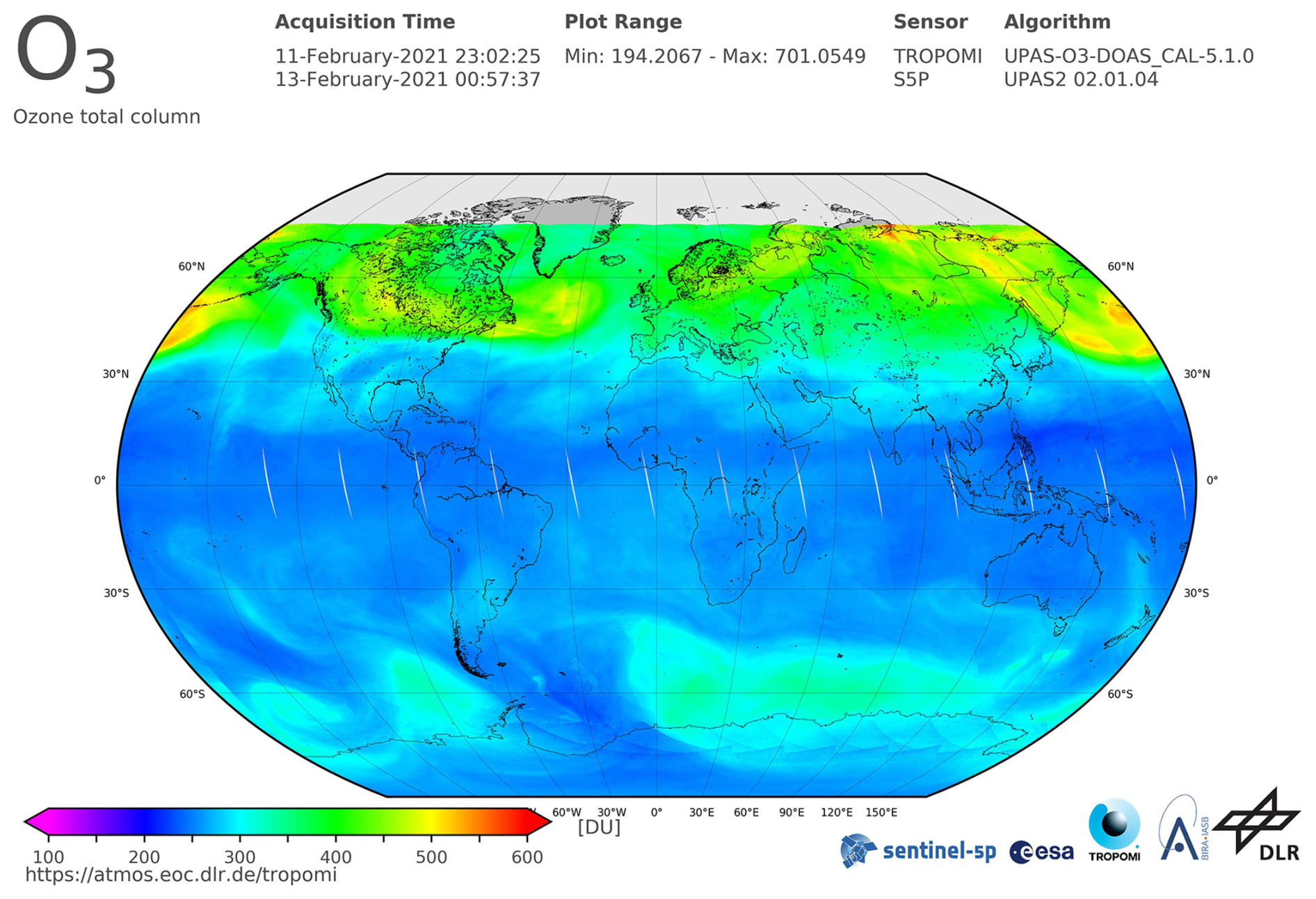
Figure 1 TCO by TROPOMI/S5P from 3 to 5 November 2020 shows ozone-poor air masses above the North Atlantic as an example of a streamer event for further analysis. Colours (from violet to red) indicate the total ozone column concentrations (from low to high) in Dobson units. Source: DLR, CC-BY 3.0.

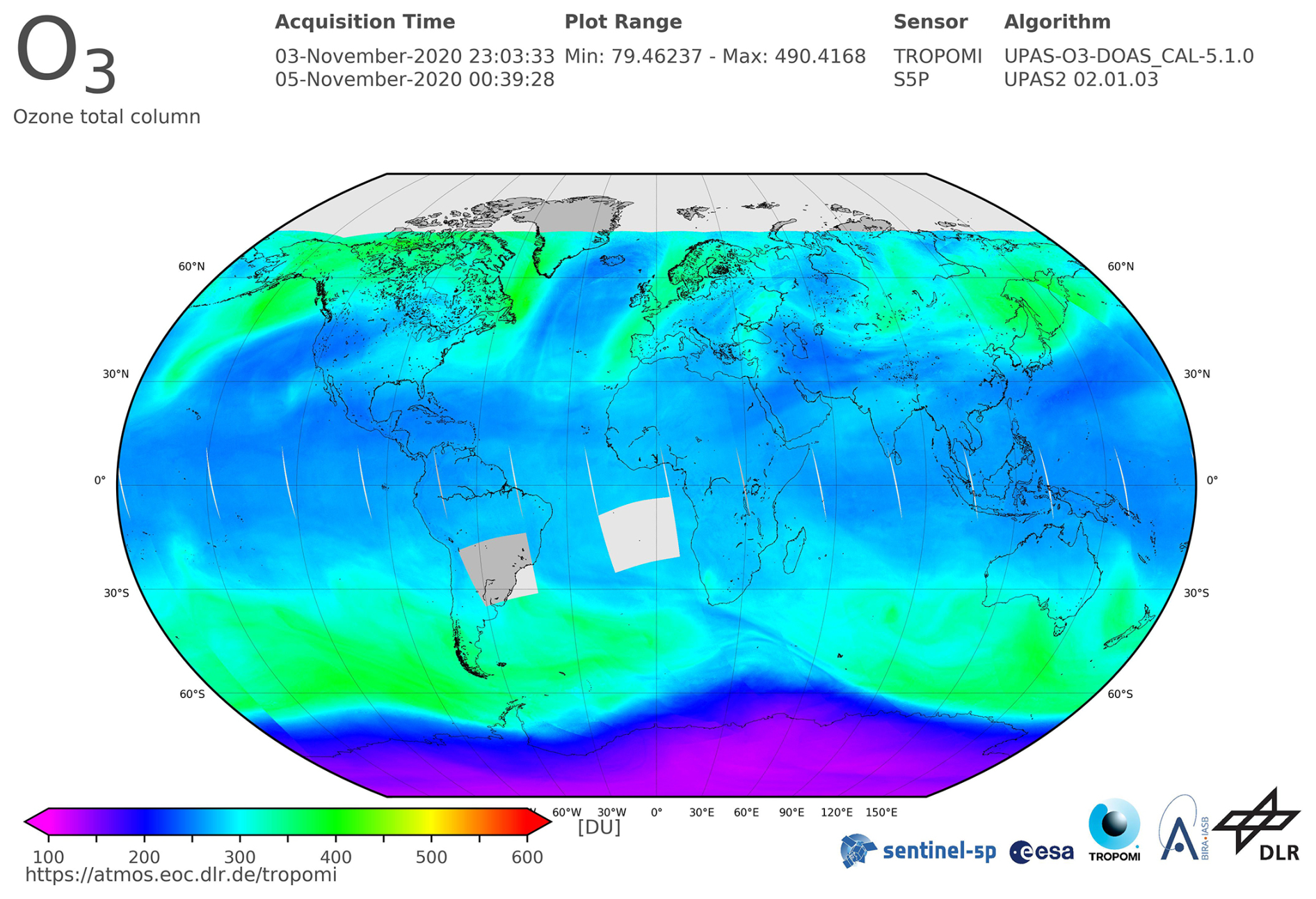
Figure 2 TCO by TROPOMI/S5P from 11 to 13 February 2020 as an example of calm atmospheric dynamics. A clear meridional gradient of ozone can be observed in the Northern Hemisphere without large-scale wave structures. Colours (from violet to red) indicate the total ozone column concentrations (from low to high) in Dobson units. Source: DLR, CC-BY 3.0.

The streamer events are selected by eye for this study (for results, see Table 1) using the TO₃ global maps from January 2020 to March 2021. As planetary waves are permanently disturbing the atmospheric dynamic of the higher troposphere–lower stratosphere, smaller-scale streamers in particular can be observed almost every day, and the identification of streamer events becomes subjective. We therefore focus on a few events which are comparatively strong in their evolution from our perspective. Moreover, we focus on streamer events above the North Atlantic. Whenever additional streamer events occur somewhere other than over the North Atlantic region with comparable spatiotemporal extent, we eliminate this date from consideration as a streamer event. We assume that the effects of the streamers superimpose, and a distinct backtracking to the streamer over the North Atlantic is possible. This means that the analysis of the streamer events can be blurred to some extent.

Table 1 Streamer events above the North Atlantic from January 2020 until March 2021 and related start and end dates (two left columns, dd.mm.yyyy). Calm periods are listed in the two columns on the right.

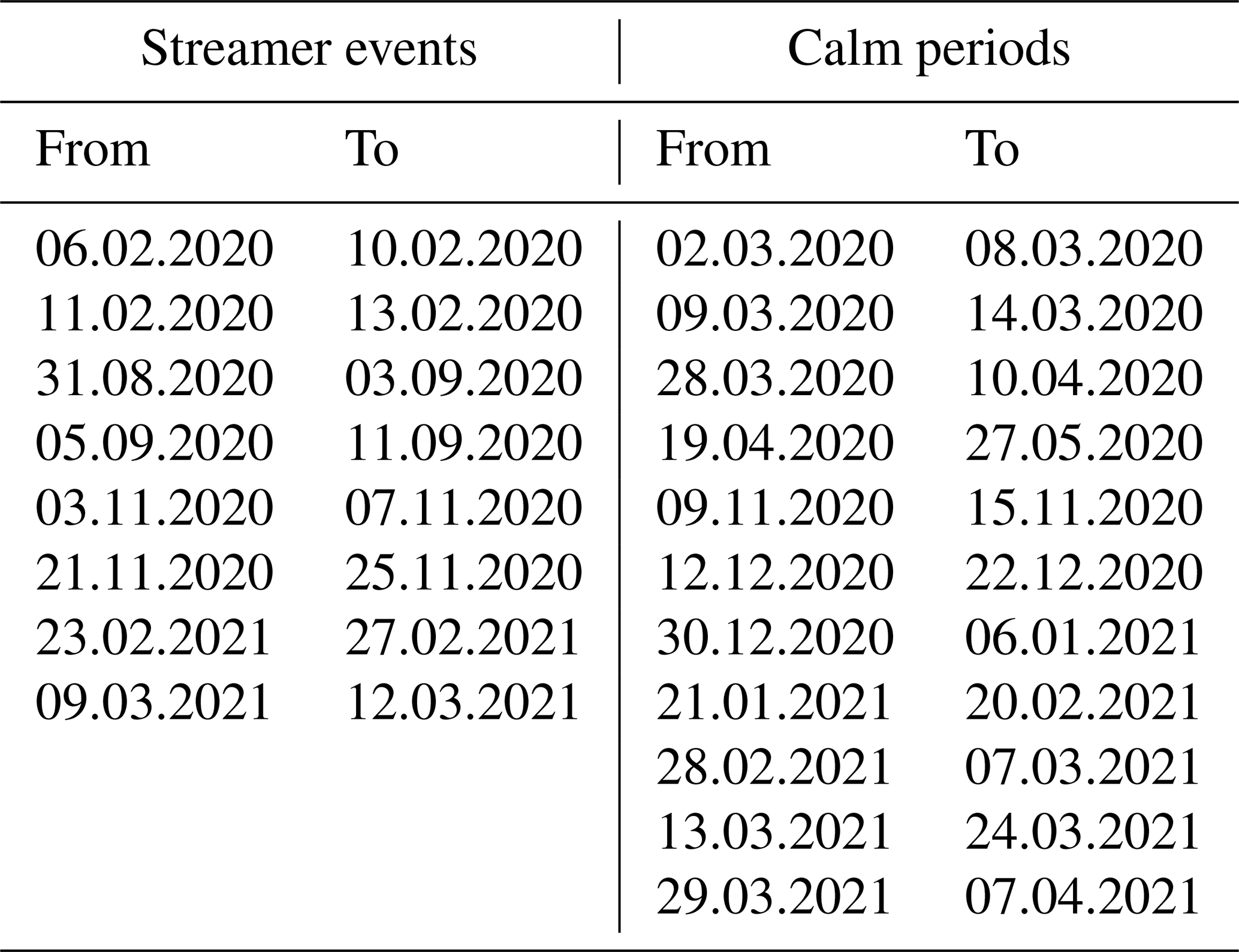
We consider dates from January 2020 to April 2021. In general, planetary waves drive the Brewer–Dobson Circulation in the stratosphere during winter, and ozone-poor air masses are transported northward. Northern Hemisphere streamer events are therefore detected between September and March. The streamer events are distinguished if they have a large spatial size and high intensity (low TO₃ concentration) and if air masses are irreversibly mixed into the surrounding atmosphere. All the selected events persist for several days but no longer than 10 d.

To evaluate whether streamer events affect the smaller-scale atmospheric dynamics, calm events are also identified through subjective criteria. These events serve as a background reference for streamer events, since large-scale spatial structures are absent in their TO₃. The events are selected when the meridional gradient of ozone concentrations from the Equator to the polar region in the Northern Hemisphere exhibits minimal longitudinal variation. Examples of calm atmospheric dynamics are listed in Table 1 (right).

Figure 1 shows the TCO from TROPOMI/S5P integrated from 3 to 5 November 2020. Ozone-poor air masses (blue) are located above the North Atlantic from 30 to 70° N along with smaller-scale ozone-poor air masses above western North America and Central Asia. The TO₃ concentration is disturbed by planetary waves around latitude circles, which lead to wave structures being visible, especially at the transition of blue to green colours. A large streamer event of ozone-poor air masses is detected over the North Atlantic. A small streamer can be detected over western North America. There are also ozone-poor air masses above eastern Europe. The temporal evolution shows that the ozone-poor air masses above eastern Europe are due to a decaying streamer, which evolved several days earlier. As planetary waves more or less permanently disturb the atmospheric dynamics, smaller-scale streamers in particular can be detected almost every day. In this example, the streamer event above the North Atlantic is the largest. Therefore, we consider this event for the further analysis.

Figure 2 shows the TCO from TROPOMI/S5P from 11 to 13 February 2020. The event is characterized by a strong meridional gradient from the equatorial to polar region in the Northern Hemisphere with almost no longitudinal variation. Therefore, we regard this event as an example of the calm period for further analysis.

Two stations from the Czech microbarograph network (Bondár et al., 2022) are involved in the study – the large-aperture array WBCI (50.25° N, 12.44° E) and the small-aperture array PVCI (50.52° N, 14.57° E). To study the propagation of GWs and long-period infrasound (from acoustic cut-off up to about 2.5 s), pressure recordings at WBCI are utilized. Four sensors of the WBCI array are arranged in a tetragon. The inter-element distances of 4–10 km provide optimum performance in the infrasound frequency range from the acoustic cut-off frequency of 0.0033 to 0.0068 Hz (Garcès, 2013). The WBCI array, with its large inter-element distances, has a unique configuration compared to the arrays of the International Monitoring System of the Comprehensive Nuclear Test Ban Treaty Organisation, which are for infrasound monitoring in the frequency band of 0.02–4 Hz (Marty, 2019). Each array element at WBCI is equipped with an absolute microbarometer of Paroscientific 6000-16B-IS with parts per billion resolution. A GPS receiver is used for time stamping. Data are stored with a sampling rate of 50 Hz. For infrasound monitoring, WBCI data are resampled at a sampling rate of 10 Hz. To detect and analyse GWs, 1 min mean values of the absolute pressure data are used.

The small-aperture array PVCI provides optimal detection precision in the frequency range of 0.14–3.4 Hz (Garcès, 2013). Three sensors are arranged in an equilateral triangle; the array aperture is 200 m. The differential infrasound gauge sensors of ISGM03, manufactured by the Scientific and Technical Centre, give a flat response in the frequency range of 0.02–4 Hz. A GPS receiver is used for time stamping. The data are stored with a sampling frequency of 25 Hz. This sampling rate is also used in regular processing of infrasound detections at PVCI.

Table 2 Main parameters of the DTK-GPMCC configurations for the arrays PVCI and WBCI.

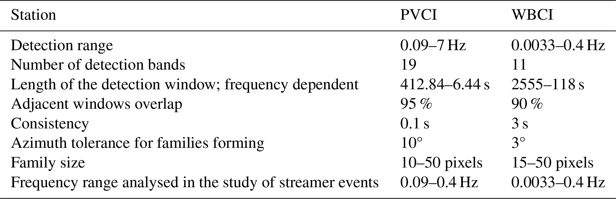
Infrasound detections are processed using DTK-GPMCC software, the core of which is the progressive multi-channel correlation (PMCC) detection algorithm (Cansi, 1995; Le Pichon and Cansi, 2003). PMCC analyses pressure recordings from an infrasound array and looks for coherent signals in overlapping time windows in several frequency bands (Le Pichon and Cansi, 2003). An elementary detection with the PMCC, or the detection pixel, is declared in the time–frequency window, when signal correlation and consistency criteria are met. Detection pixels are grouped into the detection families based on a similar time, frequency, azimuth of signal arrival, and signal trace velocity (Brachet et al., 2010). The arrival parameters of the detected infrasound are stored in the detection bulletins. The parameters of interest for the present study include time of arrival, azimuth of arrival, trace velocity, frequency, and amplitude. The PMCC configuration is set on an individual basis and is optimized for the given array (Brachet et al., 2010; Garcès, 2013; Szuberla and Olson, 2004); the main parameters of the DTK-GPMCC settings for the arrays PVCI and WBCI are given in Table 2.

InfraGA/GeoAc ray tracing tools are employed to study infrasound ducting in the atmosphere (Blom and Waxler, 2012; Blom, 2019). Infrasound ray tracing provides an easy-to-interpret approximation of infrasound propagation and can help to identify possible modifications of atmospheric waveguides above the eastern Atlantic and western Europe during streamer events. It can also show whether the streamer event influences reach Central Europe. Ray tracing is employed in our study for the purpose of identifying azimuths and distances from the source that can be influenced by the streamer event. Hence, it can reveal whether these influences reach Central Europe directly or whether the signals are ducted to the region through the waveguide in the upper stratosphere or thermosphere, as in quiet periods. InfraGA/GeoAc provides simulations of signal propagation from a point source; propagation through the range-dependent atmosphere is modelled in the present study. Atmospheric characteristics are obtained from the G2S model (Drob et al., 2003). Vertical profiles of temperature, zonal and meridional winds, density, and pressure are an input for InfraGA/GeoAc. The grid of the profiles covers the area from 45 to 65° N and from 30° W to 22.5° E; the latitudinal step is 5°, and the longitudinal step is 7.5°.

Propagation of GWs in the thermosphere/ionosphere is studied using the multi-point and multi-frequency continuous Doppler sounding system located in Czechia. Its advantage is a high time resolution (around 10 s) relative to ionospheric sounders (ionosondes) that measure the profile of electron densities in the ionosphere. Observed frequency shifts are due to the motion and electron density changes in the ionospheric plasma, caused for example by interaction with atmospheric waves propagating in the neutral atmosphere, with which the ionosphere (above ∼ 80 km) merges. The sounding radio signal is reflected at the height, where its frequency matches the so-called local plasma frequency, which is determined by the local electron density. Therefore, the reflection height changes during the day and depends on the sounding frequency. Significant Doppler shifts, usable for analysis, are obtained if the signal is reflected from the so-called ionospheric F2 layer (approximately 200–300 km). Several sounding frequencies are used in Czechia. The 3.59 MHz sounding was mostly effective at night, while the 4.65 MHz sounding provided good daytime data during the period analysed. The propagation characteristics of GWs are calculated from the time delays between signals observed at the respective sounding paths (reflection points for each transmitter–receiver pair), assuming that the reflection points are at the midpoints between each transmitter and receiver. A 60 or 90 min long time interval is usually used to calculate the velocities and azimuth of the observed waves. The methods are described in detail by Chum and Podolská (2018). The two-dimensional (2D) version (propagation analysis in a horizontal plane only) is anticipated for most of the studies, since a 3D analysis requires simultaneous observation and signal correlation at different frequencies, which is often not the case, especially during the solar minimum. Results of a statistical investigation have recently been published in Chum et al. (2021). Identical methods of propagation analysis have been applied to investigate propagation of GWs in the troposphere based on data from the large-aperture array WBCI (here the time delays are related to the locations of individual microbarometers). All analyses are done with respect to the streamer events and calm periods shown in Table 1.

3 Results

3.1 Infrasound observations at ground microbarograph arrays WBCI and PVCI in November 2020 and March 2021

Wave activity in the infrasound frequency range of 0.0033–0.4 Hz is investigated by combining observations at the WBCI and PVCI stations. Infrasound detections at WBCI are processed in the frequency band of 0.0033–0.4 Hz. The operational range of the array is extended above the upper limit of the optimum array range; the degraded performance of WBCI at frequencies higher than 0.0068 Hz is considered. The upper limit of the analysed band is intentionally set to 0.4 Hz to cover microbaroms. PVCI detections are analysed in the frequency range of 0.09–0.4 Hz. The band partly overlaps with the detection range of the WBCI array, and at frequencies of 0.12–0.35 Hz, it is dominated by microbaroms (e.g. Campus and Christie, 2010). Unlike WBCI, PVCI provides optimal performance in the microbarom band.

Microbaroms are infrasound signals generated by a non-linear interaction of ocean waves travelling in opposite directions. Microbaroms form a wide peak around 0.2 Hz in the infrasound spectrum; their frequency corresponds to twice the frequency of sea waves. A powerful source of microbaroms is located in the North Atlantic, and the signals are regularly detected by European stations (Hupe et al., 2019). The detection capability of microbaroms from the North Atlantic is particularly high from October to March when the source becomes stronger due to stormy weather above the ocean, and signal propagation to the east from the source is supported by the stratospheric waveguide (Landès et al., 2012). From a global point of view, microbaroms are permanently present in recordings of infrasound stations worldwide.

Streamer events often occur above the North Atlantic. Thus, microbaroms propagating from the North Atlantic to continental Europe can travel through the region influenced by a streamer event, and the detections at infrasound stations in Europe can show signatures of streamer events.

We analyse infrasound observations from 3 to 25 November 2020 and from 28 February to 25 March 2021 with a focus on microbaroms. In these time intervals, adjacent streamers and calm periods occurred (Table 1). Streamer events and the calm period in the November 2020 time window are evaluated separately from those in the March 2021 time window to avoid seasonal influences. While a well-developed eastward stratospheric waveguide can be expected in November, its efficiency can decrease in March due to the seasonal reversal of stratospheric winds.

3.1.1 Infrasound observations from 3 to 25 November 2020

Two streamer events developed in November 2020. The first streamer occurred from 3 to 7 November and the second one from 21 to 25 November. The streamers were separated by a calm period from 9 to 15 November.

The most important phenomena found in the infrasound arrival parameters are fluctuating signal frequency and fluctuating signal amplitude.

WBCI provides rather sparse detections during both streamer events, and only two detection families are obtained during the 7 d calm period (Fig. 3). The frequencies near 0.2 Hz and back azimuths of 290–350° indicate that the observed signals are likely microbaroms from the North Atlantic. A decrease in the signal frequency is observed during the first streamer event. On 5–6 November from 20:00 to 05:00 UTC, the mean frequency of the north-west arrivals drops down to 0.04 Hz, below the microbarom frequency range. During the second streamer event from 21 to 25 November, the signal frequency is stable around 0.22 Hz. An increase in the amplitude from the mean value of 0.019 to 0.035 Pa is observed from 23 November at 18:00 UTC until the end of the analysed time period on 25 November at 24:00 UTC.

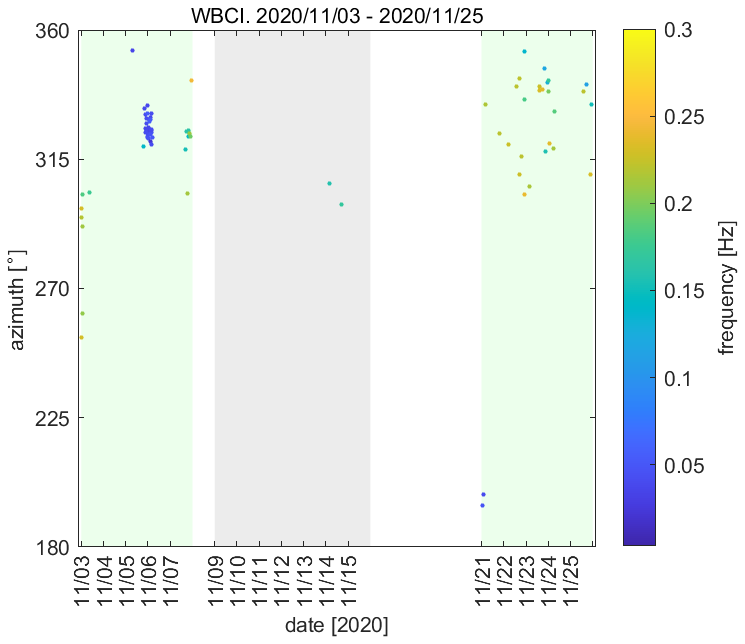
Figure 3 Infrasound observations at WBCI on 3–25 November 2020. The azimuth of signal arrivals is shown; the colour bar refers to the mean frequency of the detection family. One circle in the plot represents one detection family. The green background marks the streamer events, and the grey background marks the calm period.

Similar to the back azimuths at WBCI, PVCI detects arrivals from the north-west in the analysed frequency range of 0.09–0.4 Hz (Fig. 4). Fluctuating signal amplitudes are observed. Values around 0.020 Pa occur on 3 November. From 4 November at 18:00 UTC to 7 November at 22:30 UTC, the signals have amplitudes of around 0.089 Pa. The amplitudes decrease to values of around 0.046 Pa during the following quiet period on 9–15 November. Microbarom amplitudes fluctuate between 0.013 and 0.036 Pa (1st decile and 9th decile, respectively) during the streamer event on 21–25 November. Publicly available data, such as meteorological charts provided by the Deutscher Wetterdienst and the WAVEWATCH III^® wave-action model (WAVEWATCHIII^® Development Group, 2019), indicate that there were maritime storms in the North Atlantic within the analysed time window from 3 to 25 November 2020. Maximum heights of sea waves are predicted in the North Atlantic near the south coast of Greenland and Iceland from 5 to 6 November, from 12 to 13 November, and on 20 November. The height of combined wind waves and swell reaches 10 m. As mentioned in Sect. 3.1, it is not only the wave height but also the wave direction (waves propagating in opposite directions) that determine the microbarom source. Nevertheless, the fluctuating intensity of the microbarom source is taken into account during maritime storms. As a consequence, fluctuating microbarom amplitudes can be observed at the infrasound stations.

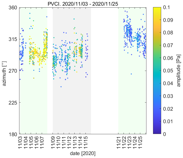
Figure 4 Infrasound observations at PVCI on 3–25 November 2020. The azimuth of signal arrival is shown; the colour bar refers to the signal amplitude. The green background marks the streamer events, and the grey background marks the calm period.

To study the propagation of signals from sources located at the surface of the North Atlantic, the InfraGA/GeoAc tools are employed. The fictitious point sources are located (1) at 55° N and 15° W, (2) at 55° N and 5° W, and (3) at 60° N and 0° longitude. The coordinates of the sources are estimated based on the position of the tropopause jet stream disturbance. Point (1) is located under the northward jet stream, point (3) under the southward jet stream, and point (2) between those two opposing branches of the jet stream disturbance; see Fig. 5.

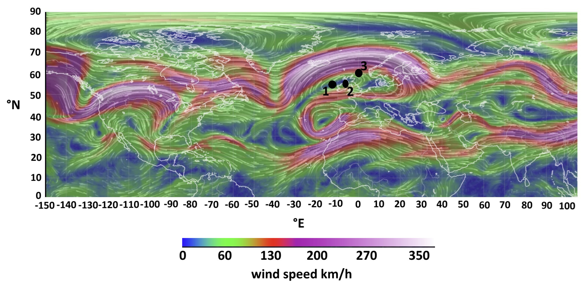
Figure 5 Wind field at the pressure level of 250 hPa on 6 November 2020 at 00:00 UTC. A disturbance of the jet stream above the eastern North Atlantic and the British Isles is caused by the streamer event. Figure taken from https://earth.nullschool.net (last access: June 2023).

A multi-azimuth simulation is run on 6 November at 00:00 UTC. The simulation is performed at the time point in the middle of the streamer event when a maximum stage of the phenomenon can be expected. Taking into account the mutual locations of the sources and the receiving arrays, eastward signal propagation is modelled. The azimuth limits are set to 0 and 180°, and the azimuth step is 3°. Rays are launched with inclinations of 2–45°; the step is 2°.

Information is obtained regarding which waveguides the signal can possibly use to arrive at the infrasound stations and their surroundings. The reason why arrivals at extended areas around the stations are considered is because signal propagation from three fictitious point sources stands in for a real source, the surface of the North Atlantic where microbaroms are generated. Therefore, the model outputs must be taken as an approximation of the real situation. The turning height and ground reflections of the 0.2 Hz signal are obtained in the multi-azimuth simulation. The results are visualized in Fig. 6 and in the Supplement. The red asterisk represents the point source. The concentric sectors of circles, i.e. regions of ensonification, show regions where the signal emitted by the source can be recorded at an infrasound station. The dots, showing signal ground reflections, are organized in a radial pattern. Each of the lines of this pattern represents one azimuth of signal propagation for which the multi-azimuth simulation is run; the azimuth step is 3°. The colours of the dots provide information about the turning height of the ray and thus also the signal ducting in the waveguides. Depending on the turning height, infrasound is subject to attenuation of variable strength when it propagates through the atmosphere. Infrasound attenuation is low in the stratospheric waveguide. Strong absorption occurs in the thermospheric waveguide; the absorption is higher at higher signal frequencies (Sutherland and Bass, 2004). To obtain the view of signal attenuation along the ray path in the vertical plane, a single azimuth simulation is employed. The single azimuth simulation is run along the azimuths from the fictitious sources (1–3) to the stations WBCI and PVCI; it is obtained for the frequencies of 0.04 and 0.2 Hz. As a reference, a multi-azimuth propagation of the 0.2 Hz signal is modelled from a source at 55° N and 15° W on the calm day of 12 November at 00:00 UTC. The time point in the middle of the calm period between two streamer events is selected to minimize possible effects of the subsiding and arising streamer events, respectively.

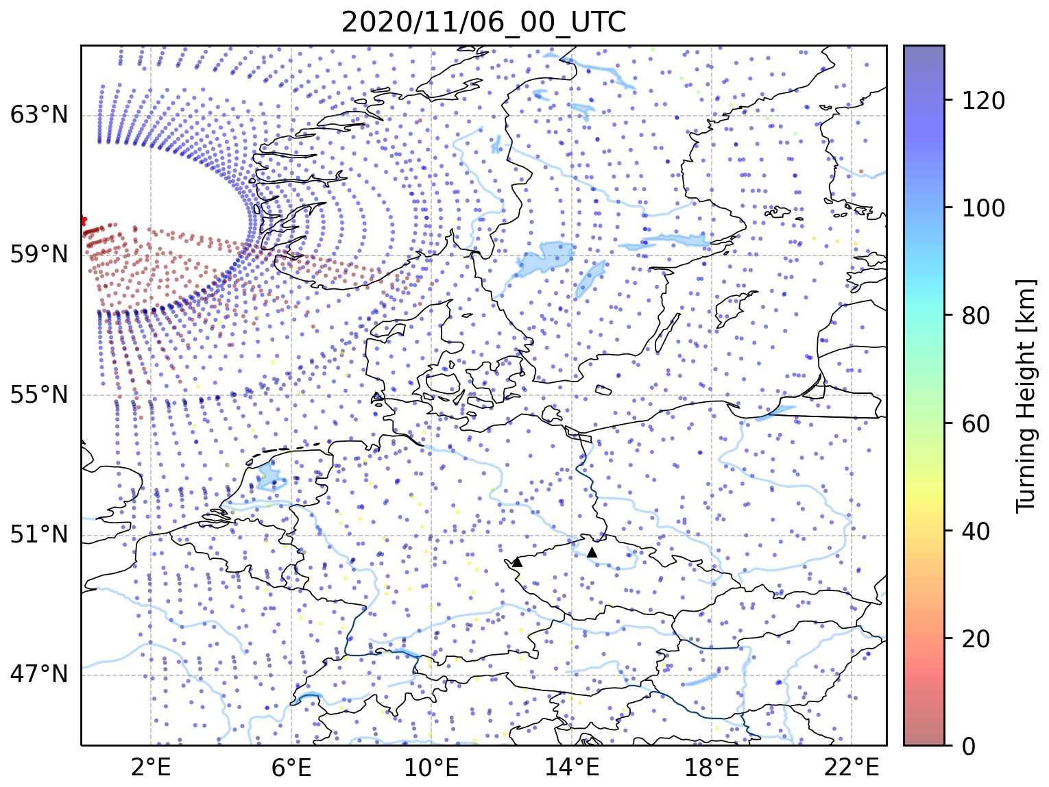
Figure 6 Modelled infrasound propagation from a point source located at 60° N and 0° longitude (red asterisk) during the streamer event on 6 November 2020 at 00:00 UTC. The colour bar refers to the turning height (maximum height) of the signal. The red colour indicates signal propagation in the waveguide formed near the tropopause (altitudes around 10 km), and arrivals through the thermospheric waveguide are shown in blue (altitudes above 100 km). The black triangles represent the WBCI (the left triangle) and PVCI (the right triangle) infrasound arrays.

First, we focus on infrasound propagation from the North Atlantic to Central Europe. Signal arrivals only through the thermospheric waveguide are enabled from the source at 60° N and 0° longitude (Fig. 6) during the streamer event on 6 November 2020 at 00:00 UTC. Stratospheric and thermospheric ducting is possible from the sources at 55° N, 15° W and 55° N, 5° W to Central Europe (Supplement). Similarly, stratospheric and thermospheric ducting is predicted from the source at 55° N, 15° W to Central Europe on the calm day of 12 November 2020 (Supplement). Signal propagation only through the thermospheric waveguide is enabled from the source at 60° N and 0° longitude (Fig. 6). The distances between the fictitious sources and the stations are 1300–2000 km. The amplitude loss of the 0.2 Hz signal in the thermospheric waveguide at these distances is 100 dB relative to the amplitude at a distance of 1 km from the source. According to the simulations, observations of the thermospheric arrivals of microbaroms are unlikely at PVCI and WBCI due to strong signal attenuation. Microbaroms apparently arrive at Central Europe through the stratospheric waveguide formed in the upper stratosphere during the streamer events and on the calm day. Indeed, arrivals from the back azimuths of 285–315° are dominant at PVCI from 3 to 7 November. Those back azimuths correspond to the positions of the fictitious sources at 55° N, 15° W and at 55° N, 5° W, while the back azimuth to the source at 60° N and 0° latitude is 325°. The amplitude loss of the 0.04 Hz signal at distances of 1300–2000 km from the source is 60–80 dB. In general, thermospheric arrivals of this low-frequency signal are not strictly rejected. However, in our case the 0.04 Hz signal arrives with trace velocity around 0.330 km s⁻¹ at WBCI. The low trace velocity indicates signal propagation in the troposphere–lower-stratosphere waveguide (Lonzaga, 2015).

Next, we study the influences of the streamer-event-related disturbance anywhere in the modelled region. The disturbance of the jet stream can modify signal propagation up to distances of several hundreds to thousands of kilometres from the source; the influenced azimuth range is limited. Signals from the source at 55° N and 15° W can propagate in the tropopause waveguide in azimuths between 10 and 60° up to a distance of ∼ 1000 km. The amplitude loss of the 0.2 Hz signal at a distance of 1000 km is 60–70 dB relative to the amplitude 1 km from the source. The southward branch of the jet stream disturbance enables infrasound propagation in the tropospheric waveguide in azimuths of 100–160° from the source at 60° N, 0° longitude. The maximum distance that the signal can travel in the south-east direction is ∼ 600 km. The amplitude loss of the 0.2 Hz signal at a distance of 600 km is 60 dB relative to the amplitude 1 km from the source.

The observations and the model outputs during the November 2020 event can be summarized as follows: infrasound arrives from sources in the North Atlantic to Central Europe mainly through the stratospheric waveguide formed between the ground and upper stratosphere. The jet stream disturbance above the eastern North Atlantic does not have an impact on infrasound arrivals in Central Europe on 6 November 2020 at 00:00 UTC. Fluctuating signal amplitudes are likely a consequence of the fluctuating intensity of the microbarom source during maritime storms. The decrease in signal frequency at WBCI is not caused by a transient change in signal ducting and the related signal filtering in the thermospheric waveguide.

3.1.2 Infrasound observations from 28 February to 24 March 2021

Another streamer event occurred from 9 to 12 March 2021, preceded and followed by calm periods from 28 February to 7 March and from 13 to 24 March, respectively.

The most important phenomenon identified in the infrasound arrival parameters is a fluctuating trace velocity.

Both WBCI and PVCI detect signals arriving from the north-west, from back azimuths of 285–310°. An increase in signal trace velocities is observed in some of the detections at WBCI during the streamer event compared to calm periods (Fig. 7). On 10 March at 00:00–06:00 UTC, trace velocities of 0.460 and 0.380 km s⁻¹ are observed from back azimuths of 270 and 310°, respectively. They are higher by 0.05–0.13 km s⁻¹ than on the calm days. On the other hand, signals from the back azimuth of 288° arrive with a trace velocity of 0.330 km s⁻¹ within the same time window, and this velocity corresponds to that on the calm days. Effects of spatial aliasing are taken into account when evaluating the detections. The signal frequencies are around 0.2 Hz, well above the range of array optimum performance. The observed different trace velocities at WBCI can therefore be a processing bias rather than a consequence of variations in signal ducting.

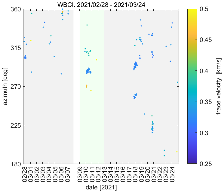
Figure 7 Infrasound observations at WBCI on 28 February–24 March 2021. The azimuth of the signal arrival is shown; the colour bar refers to the signal trace velocity. The green background marks the streamer event, and the grey background marks the calm periods.

In contrast to the WBCI observations, PVCI records a decrease in trace velocities on 10 March at 00:00–06:00 UTC (Fig. 8). Trace velocities of 0.377 km s⁻¹ are observed compared to 0.413 and 0.395 km s⁻¹ during the calm periods before and after the streamer, respectively.

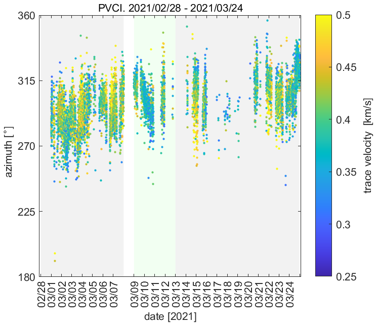
Figure 8 Infrasound observations at PVCI on 28 February–24 March 2021. The azimuth of the signal arrival is shown; the colour bar refers to the signal trace velocity. The green background marks the streamer event, and the grey background marks the calm periods.

Changes in the trace velocity can indicate changes in the refraction altitude of the signal (Lonzaga, 2015). The exact limits of the trace velocity for the given atmospheric waveguide depend on the current state of the atmosphere. We use the thresholds determined for a model atmosphere in Lonzaga (2015) as helpful indications of our further consideration: trace velocities below 0.340 km s⁻¹ indicate signal refraction in the troposphere and lower stratosphere. Trace velocities between 0.340 and 0.380 km s⁻¹ are typical of signals ducted in the waveguide between the ground and the upper stratosphere. Signals travelling in the thermospheric waveguide arrive with trace velocities larger than 0.380 km s⁻¹.

The high trace velocities recorded at PVCI disprove signal refraction in the lower stratosphere. Hence, it is unlikely that the signals arrive through a waveguide that can form at the tropopause–lower stratosphere by the effect of the streamer event.

Like in the November 2020 case, signal propagation above the eastern North Atlantic and western and Central Europe is investigated using the InfraGA/GeoAc tools. Propagation of the 0.2 Hz signal is modelled for 10 March at 03:00 UTC, in the middle of the streamer event. A source is located at 55° N, 15° W at a distance of ∼ 2000 km from the stations. This scenario represents signal propagation from the central North Atlantic. The other source is located at 55° N, 0° latitude, representing propagation of microbaroms from the North Sea. The distance from the stations is ∼ 1000 km. Both points are located under the jet stream disturbance related to a streamer event.

Eastward signal ducting is enabled in the stratospheric and thermospheric waveguides from both sources to the stations. Strong signal absorption in the thermospheric waveguide likely disables thermospheric arrivals to the PVCI and WBCI. We assume that signals ducted in the upper stratosphere are detected. The other eastward waveguide occurs near the tropopause, formed by the eastward to south-eastward jet stream above the eastern North Atlantic and western Europe at latitudes 50–60° N (Fig. 9). Signals from the source in the North Atlantic are predicted to travel in the tropopause waveguide to distances of 1000–1100 km. The signal attenuation is low in the tropopause waveguide; the relatively short distance under the waveguide influence is determined by the location and extent of the jet stream disturbance. The tropopause–lower-stratosphere arrivals can be detected mainly on the British Isles. The waveguide does not reach the PVCI and WBCI stations (see Supplement).

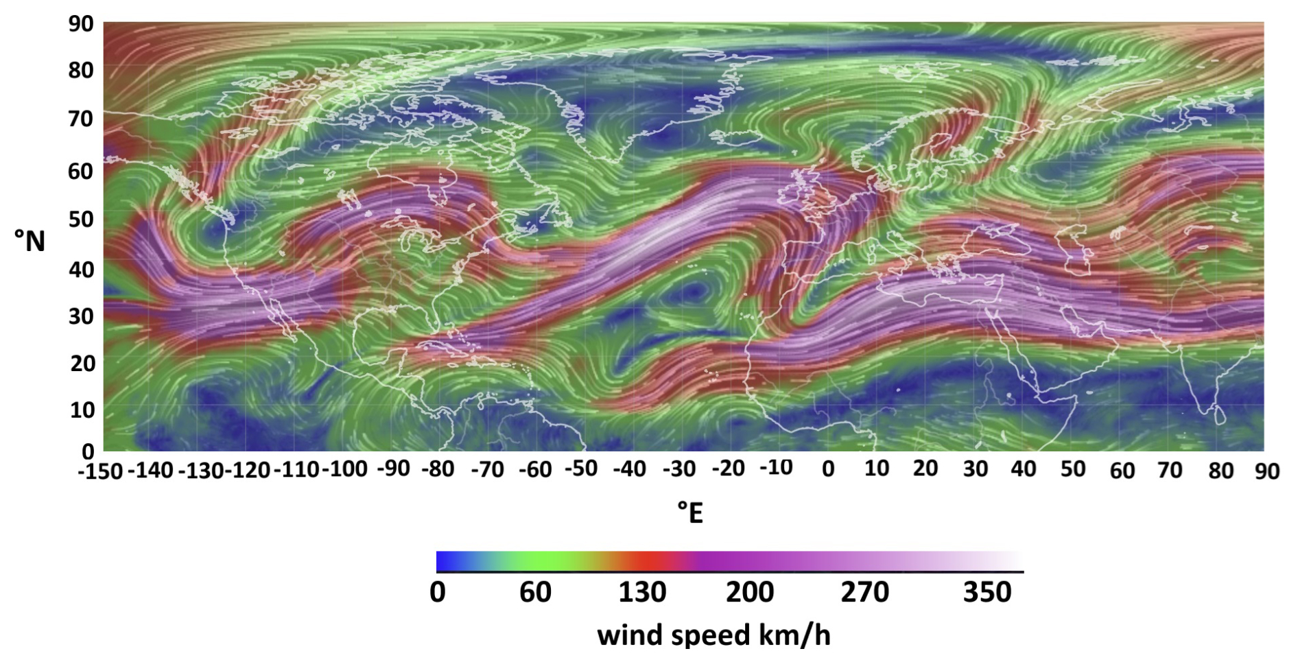
Figure 9 Wind field at the pressure level of 250 hPa on 10 March 2021 at 03:00 UTC. A disturbance of the jet stream above the eastern North Atlantic and the British Isles is caused by the streamer event. Figure taken from https://earth.nullschool.net.

Signals emitted by a source in the North Sea can propagate through the tropopause waveguide. The signals propagate to the south-east and are predicted to reach Central Europe. The tropopause–lower-stratosphere arrivals are represented by red dots in Fig. 10. The influenced regions are to the south-west from PVCI and WBCI, several hundreds of kilometres from the stations. The approximation of infrasound propagation obtained from the ray tracing is in accordance with observations. The trace velocities at PVCI of 0.377 km s⁻¹ indicate infrasound propagation in the waveguide formed between the ground and the upper stratosphere rather than in the waveguide near the tropopause.

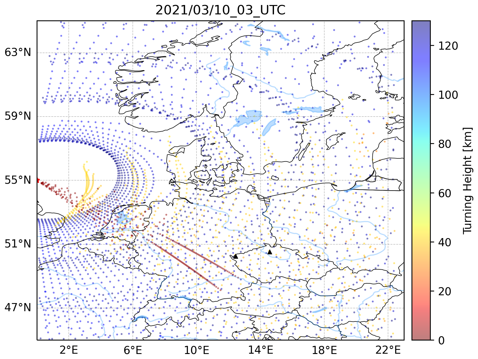
Figure 10 Modelled infrasound propagation from a point source located at 55° N and 0° longitude (red asterisk) on 10 March 2021 at 03:00 UTC. The colour bar refers to the turning height (maximum height) of the signal. The red colour indicates signal propagation in the waveguide formed near the tropopause (altitudes around 10 km), arrivals through the stratospheric waveguide are shown in yellow (altitudes around 40–50 km), and arrivals through the thermospheric waveguide are shown in blue (altitudes above 100 km). The black triangles represent the infrasound arrays WBCI (the left triangle) and PVCI (the right triangle).

Like in the November 2020 case, infrasound arrivals from the North Atlantic to the PVCI and WBCI stations in Central Europe are not influenced by the waveguide at the tropopause–lower stratosphere. Observed trace velocities fluctuate within or close above the limits that indicate infrasound propagation in the upper stratosphere during the streamer event and both adjacent quiet periods.

3.2 Results and discussion of gravity waves in the troposphere and ionosphere

3.2.1 Investigation of GWs measured on the ground by the WBCI array of microbarometers

Figure 11 shows the RMS amplitudes of pressure fluctuations in the period range 5–60 min recorded from 1 to 9 November 2020. This interval covers a distinct streamer event that occurred from 3 to 7 November. The results of the propagation analysis are shown in Fig. 12, which displays the phase velocities and azimuths of GWs. Only results that satisfied the criteria (d$v/v$ < 0.5), (dAZ < 10°), and (p_RMS > 0.02 Pa) are presented, where d$v/v$, dAZ, and p_RMS are the relative uncertainty of the GW phase velocity, the uncertainty of the azimuth, and the root mean square value of pressure fluctuations in the analysed time interval. Figure 12 demonstrates that there is a tendency for higher phase velocities and occurrence of different azimuths during the streamer event. Therefore, it is useful to compare the GW characteristics during streamer events and calm conditions.

Figure 11 Amplitude of GWs recorded by WBCI from 1 to 9 November 2020.

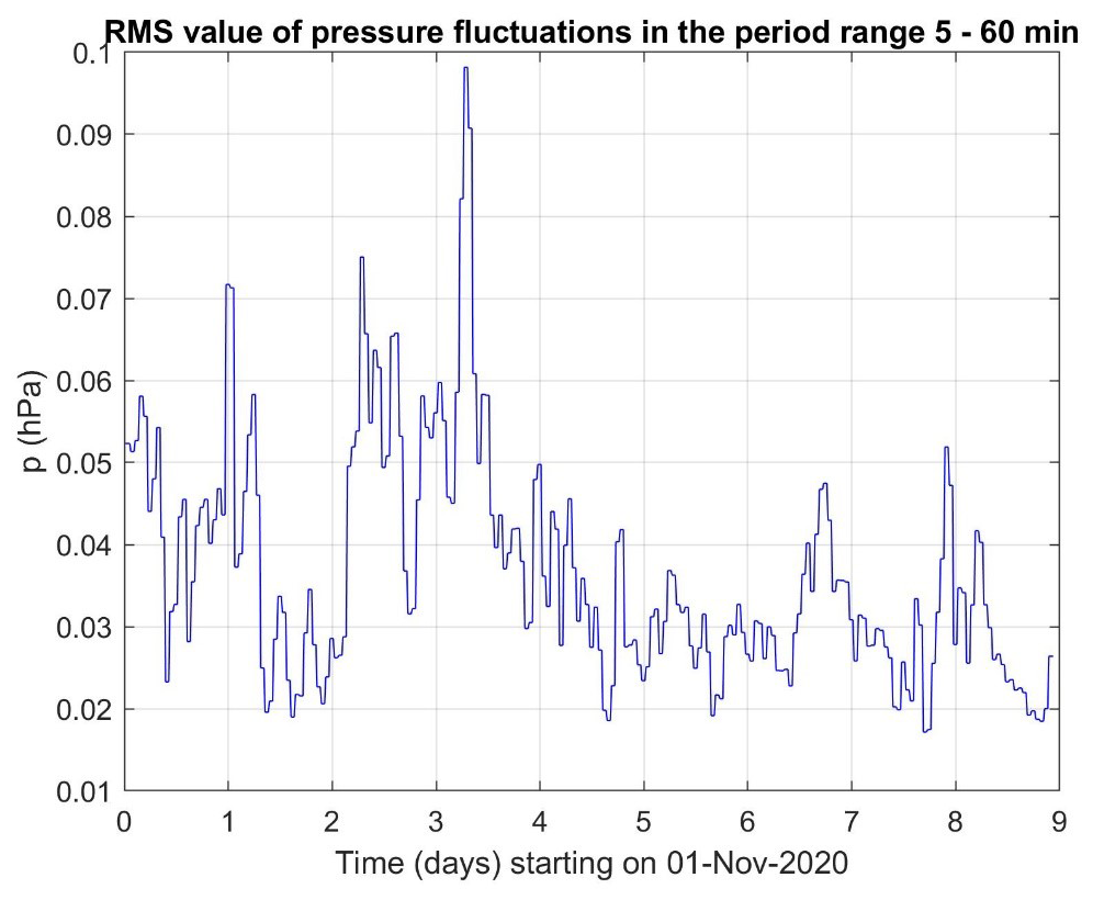
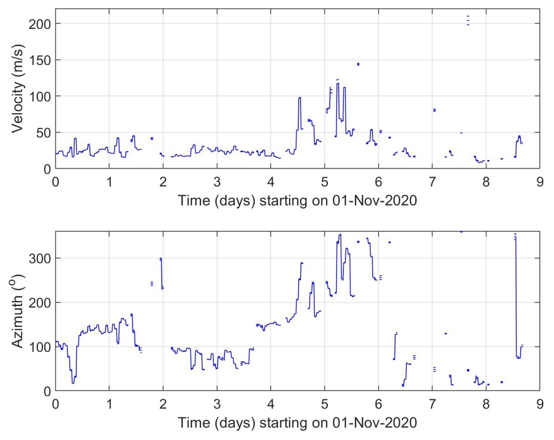
Figure 12 Propagation velocity and azimuth of GWs recorded by WBCI from 1 to 9 November 2020.

Figure 13 shows histograms obtained by a statistical analysis. The RMS amplitudes of pressure fluctuations in the period range 5–60 min, phase velocities, and azimuths were investigated separately for calm conditions (upper plots) and for streamer events listed in Table 1 (bottom plots) with a 1 h time resolution. The solid vertical lines mark lower (Q1) and upper (Q3) quartiles. The dashed vertical lines depict boundaries for large (Q3 + 1.5 ⋅ (Q3 − Q1)) and extreme (Q3 + 3 ⋅ (Q3 − Q1)) values. A difference between histograms for RMS pressure fluctuations and azimuths obtained for calm and disturbed conditions is obvious. During the streamer events the azimuths are distributed more randomly, and more extreme pressure amplitudes can be observed. A minor difference is also observed for phase velocities.

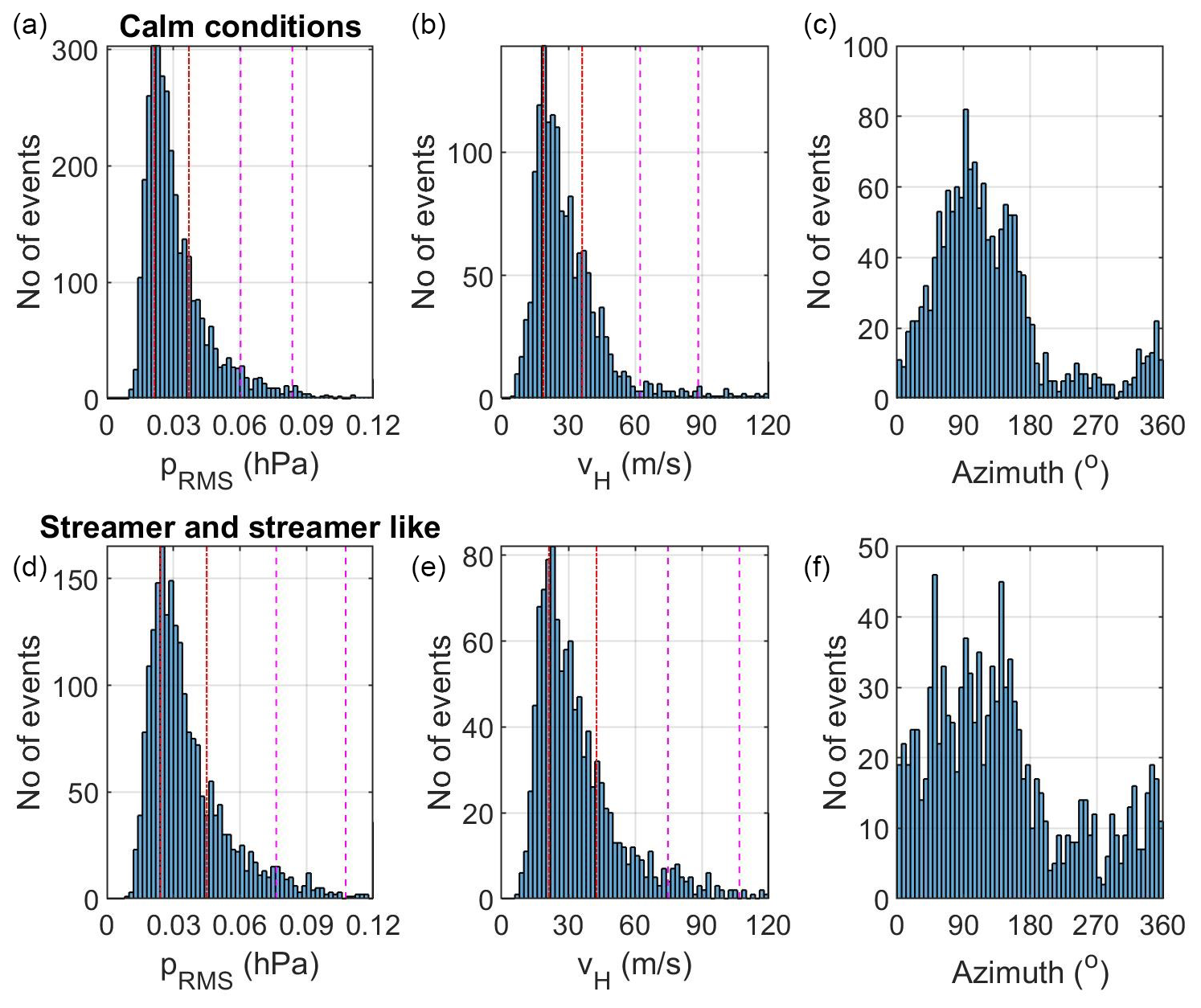
Figure 13 GW characteristics (RMS of pressure fluctuations, phase velocity, and azimuth) for calm periods (a–c) and streamer and streamer-like events (d–f) for 2020 and the winter of 2021. The vertical red lines mark the lower (Q1) and upper (Q3) quartiles. The dashed vertical magenta lines depict boundaries for large (Q3 + 1.5 ⋅ (Q3 − Q1)) and extreme (Q3 + 3 ⋅ (Q3 − Q1)) values.

3.2.2 Investigation of GWs measured in the ionosphere by a continuous Doppler sounding system (CDS)

The 2D propagation analysis of GWs was performed using the 2D versions of the methods mentioned in Sect. 2 and is described in detail by Chum and Podolská (2018). As discussed in Sect. 2 and by Chum et al. (2021), the 2D propagation analysis makes it possible to analyse a much larger number of time intervals than the 3D analysis. The propagation analysis obtained for the interval from 1 to 9 November 2020, which covers the significant streamer event that occurred from 3 to 7 November 2020, is presented in Fig. 14. Only results that satisfied the criteria (d$v/v$ < 0.2), (dAZ< 20°), (f_DRMS> 0.05 Hz), and (C_max< 0.5) are presented, where d$v/v$ is the relative uncertainty of the GW phase velocity, dAZ is the azimuth uncertainty, f_DRMS is the root mean square of the Doppler shift in the analysed time interval, and C_max is the maximum in the normalized energy map for the best beam (slowness) search. C_max is 1 for identical signals (Chum and Podolská, 2018). It is considered that signals are not sufficiently correlated (coherent) for reliable propagation analysis if C_max < 0.5 (Chum et al., 2021). The velocities and azimuth obtained by the observation at 3.59 MHz are in red, whereas the values based on measurements at 4.65 MHz are in blue. Obviously, the observations at 3.59 MHz mostly correspond to the nighttime, whereas observations at 4.65 MHz were mostly made during the daytime. The 4.65 MHz signal did not reflect from the ionosphere (escaped to outer space) at night due to the low critical frequency of the ionosphere. On the other hand, the 3.59 MHz signal mostly reflected during the day from the ionospheric E layer, and the Doppler shift was negligible and difficult to analyse. The GWs usually propagated roughly poleward at night and roughly equatorward during the daytime. This is fully consistent with the statistical investigation by Chum et al. (2021), which showed that the propagation directions of GWs in the ionosphere exhibit diurnal and seasonal behaviour and are mainly controlled by the neutral winds in the thermosphere.

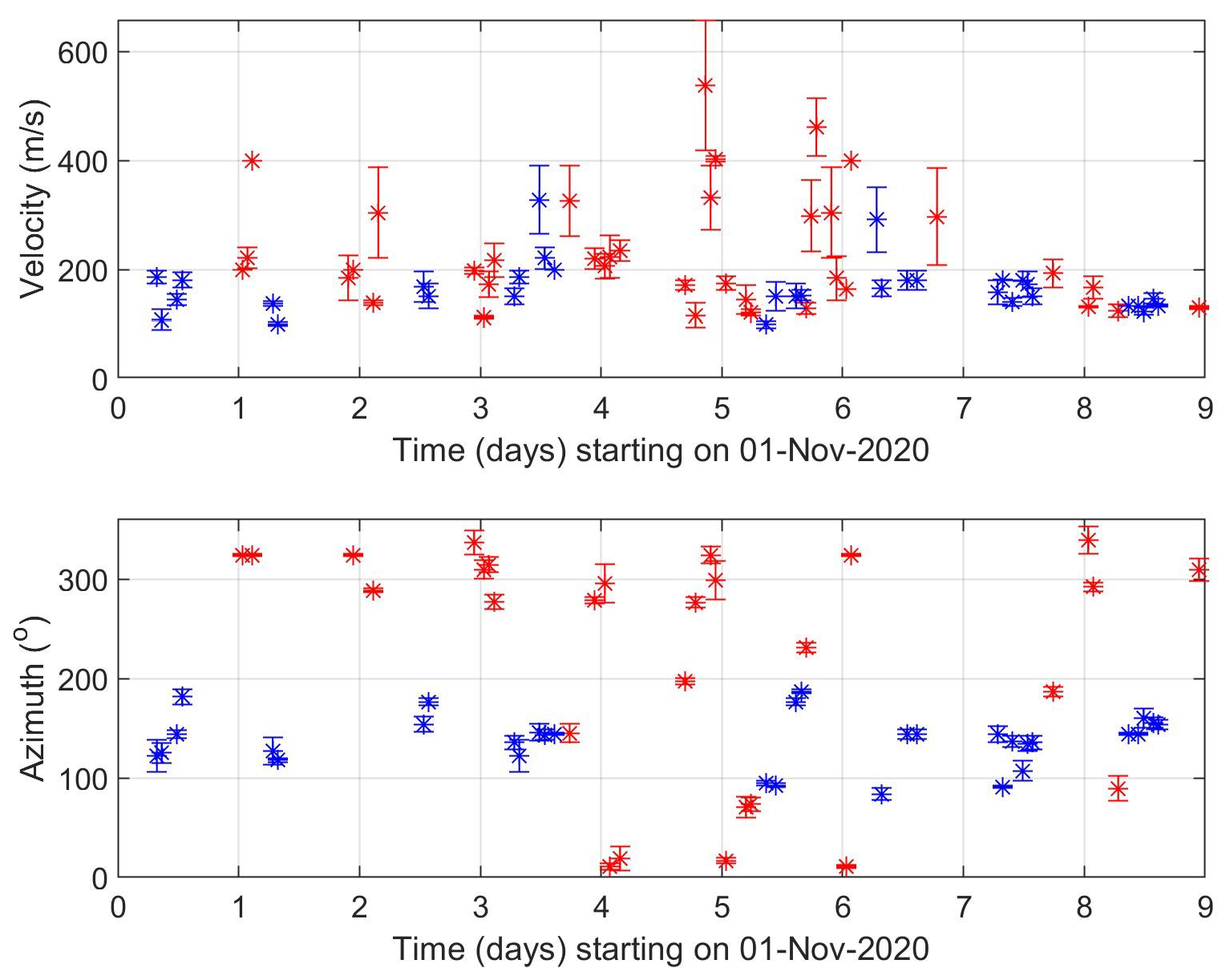
Figure 14 Propagation velocity and azimuth of GWs in the ionosphere obtained using CDS measurements from 1 to 9 November 2020. The velocities and azimuth obtained by the observation at 3.59 MHz are in red, whereas the values based on measurements at 4.65 MHz are in blue.

Based on the analysis of the GWs observed in the ionosphere during the streamer event and in the previous statistical analysis, we conclude that no obvious signature related to streamer events was observed for the propagation of GWs to the ionosphere.

It should also be mentioned that the phase velocities of GWs measured on the ground (Fig. 8) and at heights around 200 km in the ionosphere differ. There are several reasons for this. First, the observed horizontal phase velocities depend on the elevation angle of GW propagation and on the ambient temperature, as follows from the dispersion relation (the temperature enters the dispersion relation via the buoyancy frequency and the scale height). The temperature in the ionosphere/thermosphere is several times higher than in the troposphere. The elevation angles might change during the upward propagation of GWs, depending on the wind and temperature profile. Second, GWs propagate with a tilt, not vertically upward. It is therefore highly probable that the sources of the GWs observed in the troposphere and ionosphere are different. Moreover, GWs can break during their propagation upward, and secondary gravity waves might be observed in the ionosphere.

4 Conclusion and discussion

The focus of this study was to test independent types of observations, like Doppler sounding and microbarograph measurements, for an analysis of GW behaviour during streamer events, which are strongly connected with PWs or GWs and the large-scale mass transport of ozone, and that is why it can be very interesting for studies of atmospheric dynamics.

We also investigated infrasound propagation during streamer events, since modifications of infrasound ducting in the atmosphere can be expected in these periods. We evaluated infrasound detections at two microbarograph arrays in Central Europe during streamer events and compared them with observations during adjacent quiet periods. To obtain an overview of infrasound propagation from the source region to the region of observations, InfraGA/GeoAc ray tracing tools (Blom and Waxler, 2012; Blom, 2019) were employed. In general, geometric acoustic approximation (ray tracing) and the full-wave models are used for simulations of infrasound propagation through the atmosphere. The great advantage of the full-wave models is that they capture the leaking of energy between the waveguides. Waxler and Assink (2019) emphasize in particular energy leaking between the tropospheric and stratospheric waveguides. Geometrical acoustic approximation provides an easy-to-interpret model of infrasound propagation in the atmosphere at lower computational costs compared to the full-wave models. Its disadvantage is that the geometrical acoustic approximation assumes no energy propagation in the forbidden regions (for details, see e.g. Waxler and Assink, 2019) and thus provides a model of infrasound propagation in separated waveguides. Available methods of infrasound propagation simulations are discussed in detail by Waxler and Assink (2019). The approximation of atmospheric wave ducts provided by the ray tracing was sufficient for the purpose of our study; we aimed to obtain an elemental picture of infrasound propagation during the periods of interest. This means to identify which waveguides are formed, their directivity, and their spatial extent.

InfraGA/GeoAc predicts that a waveguide develops at the tropopause during the analysed streamer events in November 2020 and March 2021, the direction of which is determined by the disturbed jet stream. The tropopause waveguide ducts infrasound up to distances of several hundreds to thousands of kilometres from the source in a limited azimuth range. The azimuth sector of the extent of 50–60° is influenced in the analysed cases.

In accordance with the model predictions, phenomena that can be unambiguously attributed to streamer event effects were not found in infrasound detections at the PVCI and WBCI infrasound stations during the studied cases. We assume that the observability of streamer event signatures in infrasound arrival parameters depends on the mutual position of the source, the streamer event disturbance of the tropopause jet stream, and the infrasound station. It can be recommended that future studies use a dense network of infrasound arrays that covers various directions and distances from the streamer event. Due to the typical occurrence of the streamer events over the North Atlantic, infrasound stations in western Europe are of particular interest.

Supplementary ground-based measurements of GWs using the WBCI array in the troposphere showed that GW propagation azimuths were more random during streamer and streamer-like events compared to those observed during calm conditions, as can be seen from the plots in Fig. 13. On the other hand, the GW propagation characteristics observed in the ionosphere by CDS during streamer events did not differ from those expected for the given time period, based on previous statistical studies (Chum et al., 2021).

The results therefore indicate that streamers in the stratosphere might lead to changes in wave propagation in the troposphere. The impact on the ionosphere was not confirmed but cannot be excluded due to sparse and localized observations of GW activity. In general, to validate the preliminary results obtained in this study, a denser measurement network and more streamer events need to be analysed.