Predictions of failed satellite retrieval of air quality using machine learning

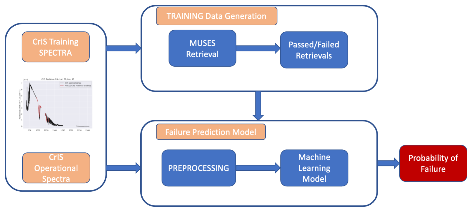
The growing fleet of Earth observation (EO) satellites is capturing unprecedented quantities of information about the concentration and distribution of trace gases in the Earth's atmosphere. Depending on the instrument and algorithm, the yield of good remote soundings can be a few percent owing to interferences such as clouds, non-linearities in the retrieval algorithm, and systematic errors in the radiative transfer algorithm, leading to inefficient use of computational resources. In this study, we investigate machine learning (ML) techniques to predict failures in the trace gas retrieval process based upon the input satellite radiances alone, allowing for efficient production of good-quality data. We apply this technique to ozone and other retrievals using measurements from multiple satellites: the Suomi National Polar-orbiting Partnership Cross-Track Infrared Sounder (Suomi NPP CrIS) and joint retrievals from the Atmospheric Infrared Sounder (AIRS) Ozone Monitoring Instrument (OMI). Retrievals are performed using the MUlti-SpEctra, MUlti-SpEcies, Multi-SEnsors (MUSES) algorithm. With this tool, we can identify 80 % of ozone retrieval failures using the MUSES algorithm at a cost of 20 % false positives from CrIS. For AIRS-OMI, 98 % of ozone retrieval failures are identified at a cost of 2 % false positives. The ML tool is simple to generate and takes <0.1 s to assess each measured spectrum. The results suggest that this tool can be applied to data from many EO satellites and can reduce the processing load for current and future instruments.

1 Introduction

The advent of geostationary Earth observation (EO) satellites designed to provide hourly estimates of trace gas concentrations is a significant step forward in understanding global problems such as climate change and air pollution (NASES, 2018; Szopa et al., 2021). These satellites, such as Sentinel-4 on MetOp (Ingmann et al., 2012); Tropospheric Emissions: Monitoring of Pollution (TEMPO) (Zoogman et al., 2017); the Geostationary Environmental Monitoring Spectrometer (GEMS) (Nicks et al., 2018), the Geostationary Carbon Cycle Observatory (GeoCarb) (Moore III et al., 2018); AIM-North (Nassar et al., 2019), and Geostationary Extended Orbits (GeoXO; NOAA, 2025), are expected to capture huge quantities of measurements over many years. In addition, low Earth-orbiting satellites, such as the Suomi National Polar-orbiting Partnership Cross-Track Infrared Sounder (Suomi NPP CrIS), capture millions of measurements daily. This results in a significant challenge, i.e. the timeliness of generating trace gas concentrations. The optimal estimation retrieval algorithms used to convert measured spectra into trace gas concentrations (Rodgers, 2000; Worden et al., 2007) are resource intensive, typically requiring several minutes to generate a single estimate. Therefore, one of the key challenges in exploiting the capabilities of the geostationary EO satellites is not in making the measurements but rather in the ability to process, store, and interpret the satellite measurements in a timely manner. This is recognised in the satellite retrieval community, with the TROPOMI total column ozone retrieval algorithm consisting of two aspects, a near-real-time (NRT) version and an offline version, where the NRT version sacrifices accuracy for speed (Garane et al., 2019).

There has been significant effort dedicated to improving the speed of retrieval algorithms (Hedelt et al., 2019; Noël et al., 2022). The largest bottleneck is found in the radiative transfer models (RTMs), e.g. Vector LInearized Discrete Ordinate Radiative Transfer (VLIDORT; Spurr, 2006). RTMs simulate the transfer of radiation through the atmosphere and are fundamental components of any physics-based retrieval algorithm (Rodgers, 2000). Typical speed-up methods include replacing the whole or part of the RTM with an approximation such as an emulator and/or neural network (NN) (e.g. Rivera et al., 2015; Brence et al., 2023; Brodrick et al., 2021; Efremenko et al., 2014; Himes et al., 2020; Pal et al., 2019) or a look-up table (Loyola et al., 2020). Other methods include simplifying the input and output of the RTM using techniques such as principal component analysis (PCA) (Jindal et al., 2016) or reducing the number of monochromatic calculations (Liu et al., 2020; Mauceri et al., 2022; Natraj et al., 2005, 2010; Somkuti et al., 2017).

However, a significant drain on resources while processing large quantities of spectra still remains, namely the fact that the retrieval process frequently yields poor-quality results, where the output data must be discarded. These retrieval failures can occur for a variety of reasons, for example, excessive cloud in the light path, a low signal-to-noise ratio (SNR), or a poor-quality fit, depending on the algorithm in question (Kulawik et al., 2021). These failed retrievals require the same processing resources as good-quality retrievals; if those spectra that yield failed retrievals could be screened and removed from the processing chain then significant processing overhead could be saved.

In this study, we investigate machine learning (ML) methods for predicting failed trace gas retrievals using measured satellite spectra prior to full retrieval. Some research has been conducted on the pre-selection or filtering of trace gas retrievals using ML methods based on genetic algorithms (Mandrake et al., 2013). In addition, other examples exist where NNs are used to improve the throughput from retrieval algorithms (Mendonca et al., 2021). However, in the case of Mendonca et al. (2021), the method is applied purely over northern latitudes for a specific solution not applicable to most satellite instruments, while the solution presented in this paper will be applicable to any satellite instrument on a global basis.

The primary source of data for this study is spectra from the satellite instruments Suomi NPP CrIS (Han et al., 2013), the Atmospheric Infrared Sounder (AIRS) on the Aqua satellite (Aumann et al., 2003), and the Ozone Monitoring Instrument (OMI) on Aura. Trace gas retrievals and their associated quality statistics are generated using the MUlti-SpEctra, MUlti-SpEcies, Multi-SEnsors (MUSES) retrieval algorithm (Worden et al., 2007; Luo et al., 2013; Fu et al., 2013, 2016, 2018; Malina et al., 2024), which is a core part of the TRopospheric Ozone and its Precursors from Earth System Sounding (TROPESS) project. TROPESS produces long-term Earth science data records with uncertainties and observation operators, which are freely available (https://tes.jpl.nasa.gov/tropess/get-data/products/, last access: 8 April 2025). The MUSES algorithm has considerable heritage for instruments sensitive to a wide range of spectral regions, from ultra violet (UV) to thermal infrared (TIR) (Bowman et al., 2002; Kulawik et al., 2006, 2021; Malina et al., 2024; Worden et al., 2007; Natraj et al., 2011, 2022; Luo et al., 2013; Fu et al., 2013, 2018). The CrIS instrument was chosen for this analysis due to the high data volume and wide spectral range (allowing for multiple different products). CrIS products are currently a key component of TROPESS, where, for example, CrIS ozone retrievals have been used with reanalysis models to understand tropospheric ozone during COVID-19 lockdowns (Miyazaki et al., 2021). In addition, TROPESS–CrIS carbon monoxide products have been used to understand the impact of wildfires in Australia (Byrne et al., 2021). The joint spectral products of TROPESS from AIRS-OMI (Fu et al., 2013) were also chosen for this study due to the inclusion of the OMI UV sensitivity, which contrasts to the TIR of CrIS.

Different trace gas (e.g. ozone or carbon monoxide) retrievals use absorption in different spectral windows, meaning that each gas retrieval has different characteristics and will not fail in the same way. Therefore, we focus on three different MUSES CrIS and AIRS-OMI products in this study, namely ozone (O₃), carbon monoxide (CO), and the temperature profile (TATM) to explore these differences. These products were chosen for their sensitivities in different regions of the CrIS spectral range. Further, although this study is focused on the MUSES algorithm and data from the CrIS and AIRS-OMI instruments, the methods are readily applicable to any retrieval algorithm or satellite instrument.

This paper is structured as follows: Sect. 2 describes the satellite data and atmospheric retrieval methods used in this study. Section 3 identifies the training datasets that form the core of the study, as well as the ML tools that use them. Section 4 shows the performance of the ML models, and Sect. 5 applies the ML models to a dataset not seen during training. The discussion and conclusion are presented in Sects. 6 and 7.

2 Instruments and tools

2.1 Suomi NPP CrIS

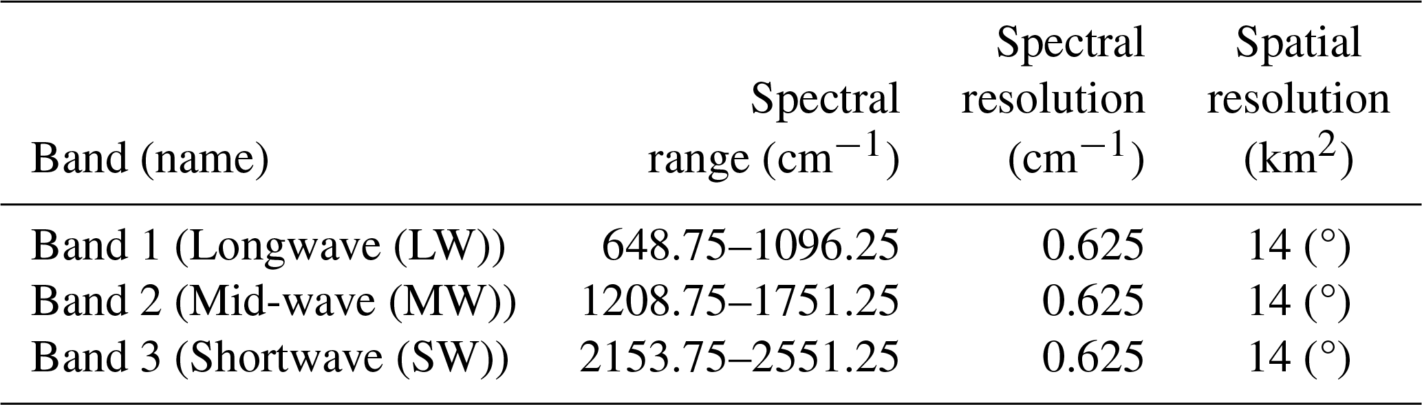
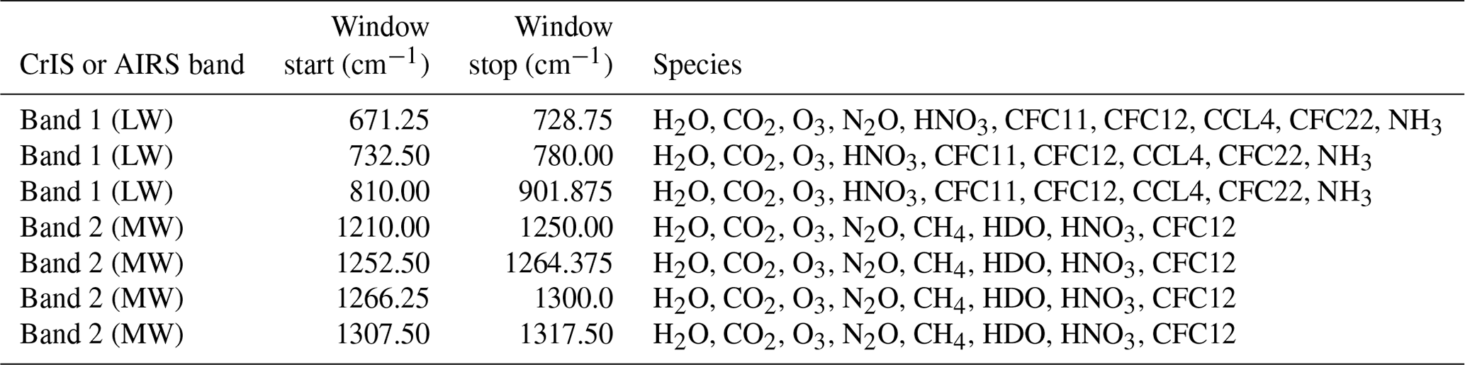
CrIS is a nadir-viewing Fourier transform spectrometer (FTS) that measures TIR radiances in three spectral bands identified in Table 1 (Han et al., 2013). Located on the Suomi NPP satellite (operational since 28 October 2011) in a near-polar, sun-synchronous, 828 km altitude orbit with a 13:30 ascending-node crossing time, CrIS provides daily global measurements, with a width of 2300 km, sampled at 30 cross-track positions, where each position consists of a 3×3 array of 14 km diameter fields of view. The wide spectral range and high spatial sampling allow CrIS to retrieve a range of atmospheric products, including trace gas products such as ozone and carbon monoxide (Fu et al., 2018; Kulawik et al., 2021; Malina et al., 2024). With the wide spectral range, multiple trace gas products from the MUSES CrIS algorithm are regularly generated as part of the TROPESS project (https://tes.jpl.nasa.gov/tropess/get-data/products/, last access: 8 April 2025, TROPESS, 2025), offering an opportunity to test the retrieval failure tool on multiple spectral windows from the same instrument.

Table 1 Characteristics of the Suomi NPP CrIS bands.

2.2 AIRS-OMI

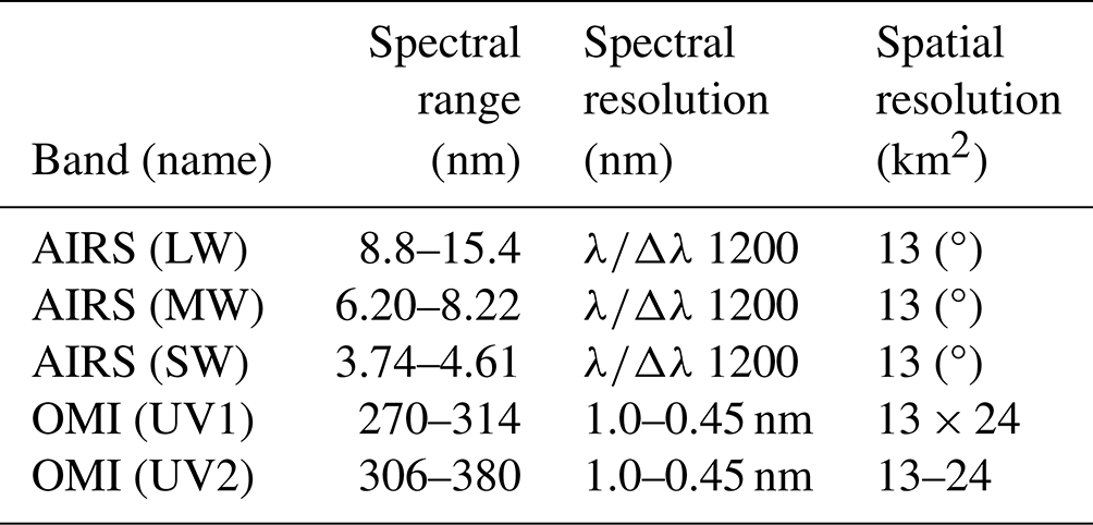
AIRS is a grating spectrometer on board the Aqua satellite that measures TIR emissions in the 650–2665 cm⁻¹ spectral range, similarly to CrIS (Aumann et al., 2003). AIRS is a cross-track scanning instrument that provides daily global coverage of multiple species, with a footprint of ∼ 13.5 km.

OMI is a nadir-viewing push broom ultraviolet–visible (UV–VIS) grating spectrometer on the AURA satellite that measures solar backscattered radiance. OMI measures in the 270–500 nm wavelength range (Levelt et al., 2006). The ground pixel size of OMI at nadir is ∼ 13 × 24 km when using the 310–330 nm spectral range.

TROPESS provides a joint spectral AIRS-OMI ozone product (Fu et al., 2018), combining information from both the TIR and UV ranges. The AIRS-OMI retrieval has been extensively validated and has been used as a key component for chemical re-analysis datasets (Miyazaki et al., 2020b, a). The characteristics of AIRS and OMI are identified in Table 2.

Table 2 Characteristics of the Aqua AIRS and AURA OMI bands.

2.3 TROPESS and MUSES

2.3.1 Algorithm description

The MUSES algorithm has a long heritage in retrieving atmospheric parameters and is designed to be flexible, such that multiple trace gas retrievals from multiple instrument types are possible, including CrIS (CrIS is also on NOAA’s Joint Polar Satellite System (JPSS) NOAA-20), AIRS on Aqua, the Tropospheric Emissions Spectrometer (TES), OMI on the AURA satellite, and the TROPOspheric Monitoring Instrument on Sentinel-5P. The description and application of MUSES to these instruments can be found elsewhere (Kulawik et al., 2006; Fu et al., 2013, 2018; Kulawik et al., 2021; Bowman et al., 2006; Worden, 2004; Worden et al., 2007, 2012, 2019; Malina et al., 2024). However, to summarise, MUSES is a non-linear retrieval algorithm based on the well-established optimal estimation method (OEM) (Rodgers, 2000). To determine trace gas concentrations, MUSES optimally fits the simulated radiance output from an RTM in predetermined spectral windows to radiance measurements. The MUSES CrIS retrieval provides the following retrieval quantities: O₃, CO, TATM, H₂O, HDO, methane (CH₄), ammonia (NH₃), peroxyacetyl nitrate (PAN), and methanol (CH₃OH). A retrieval pipeline is implemented to refine atmospheric parameters prior to the retrieval of these trace gases.

2.3.2 Brief description of computational setup

The TROPESS project has access to computational facilities that include 100 s of individual cores. This processing facility typically allows for the completion of trace gas retrievals in several minutes, with multiple retrievals occurring in parallel. The time for a retrieval depends on the instrument, with AIRS-OMI taking longer than CrIS. Based on the computational facilities available and the processing times for retrievals, typically, a test dataset of around 8000 retrievals takes roughly 2 d to create. This time period gives a reference with regard to how much speed-up the TROPESS project can expect by removing retrievals from the pipeline. However, we do not refer directly to how this tool will speed up processing as this will differ depending on the processing facilities available to other institutes. The key points are how many failed retrievals are removed from the pipeline.

3 ML tools and datasets

Predicting retrieval failure is a binary classification task, where the input – in this case, an L1B spectrum – contains many continuous parameters (radiances), and the output is a single binary value, indicating a good- or bad-quality retrieval. We consider an example to be positive if its retrieval failed.

3.1 Training datasets

Two training datasets for CrIS and AIRS-OMI are employed, each made up of approximately 40 000 individual retrievals obtained over 5 d (each day contains roughly 8000 points) in the year 2020, with each day taken from a different month to capture different seasonal effects. We train a separate ML model for each MUSES product determined from each instrument: ozone, carbon monoxide, and TATM.

For CrIS training, the first vector to be passed into the ML model is one of two options: the measured spectral data for one of the specified trace gas quantities (i.e. in the spectral windows defined in Tables A1, A3, and A4 in the Appendix) or the whole CrIS spectral range. The spectroscopic effects immediately outside the spectral windows can impact the spectral windows of the target gases. We therefore assess the impact of the whole CrIS spectral range on predicting retrieval failures.

For AIRS-OMI training, only the spectral windows were used as defined in Tables A1, A2, A3, and A4. The whole spectral range was found not to have a significant impact.

The second vector input for training purposes is the quality statistics associated with the L1B spectra. Following the completion of a retrieval, the MUSES algorithm undertakes an assessment of the quality through the flagging of specific metrics. The quality flags for MUSES CrIS, AIRS, and/or AIRS-OMI ozone, carbon monoxide, and TATM retrievals are indicated in Table 4. These values are based on a statistical analysis of the retrieval data indicating the typical ranges. If any of these values are flagged for falling outside of the accepted range then the retrieval is determined to be of poor quality, tripping a master quality flag. Unique quality values are generated for each target gas and are identical for training purposes regardless of whether the spectral window or full band is used.

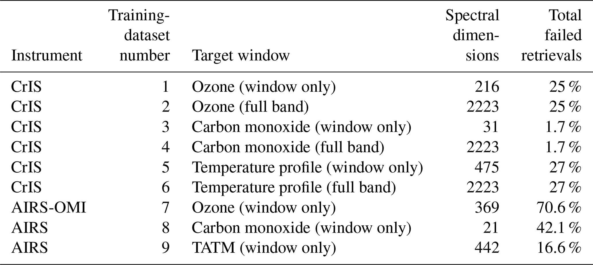
For training purposes, there are six distinct training datasets for CrIS, with each of these training datasets being drawn from the same L1B spectra but with the differences being in the spectral windows. Therefore, there are two datasets for each of the target MUSES products (ozone, carbon monoxide, and TATM), with one using the spectral windows defined in Tables A1 or A3, or A4 and with one using the full available CrIS spectral range. These are defined in Table 3 and Fig. 1.

For AIRS-OMI, there are three training sets based on the spectral windows of the products (ozone, carbon monoxide, and TATM). Note that only AIRS retrieves carbon monoxide and TATM, while the joint AIRS-OMI retrievals are used for ozone.

Table 3 Description of input training datasets.

The spectral windows defined in Table 3 for each trace gas are shown in contrast to the available CrIS spectral range in Fig. 1. Both the TATM and ozone spectral regions are largely found in the longwave (LW) and mid-wave (MW) spectral regions, with some overlap between them. Carbon monoxide is only found in a very narrow range in the shortwave (SW) spectral region.

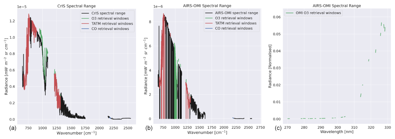
Figure 1 Example spectral windows. Panel (a) shows windows for ozone, CO, and TATM with respect to CrIS radiance. Panel (b) shows the same as the left-hand panel but for AIRS radiance. Panel (c) shows the ozone spectral windows in the OMI radiance as a part of the AIRS-OMI retrieval.

Note that numerous gaps are shown in Fig 1 for the OMI radiance values, which are due to poor-quality spectral pixels being removed from the analysis.

Table 4 List of quality flags in MUSES for CrIS and AIRS-OMI ozone, carbon monoxide, and temperature profile retrievals; all retrieval values that fall outside the specified range are flagged as bad quality. The pass rate for each instrument for 8000 retrievals on the example day of 15 June 2020 is shown. Note: n/a – not applicable.

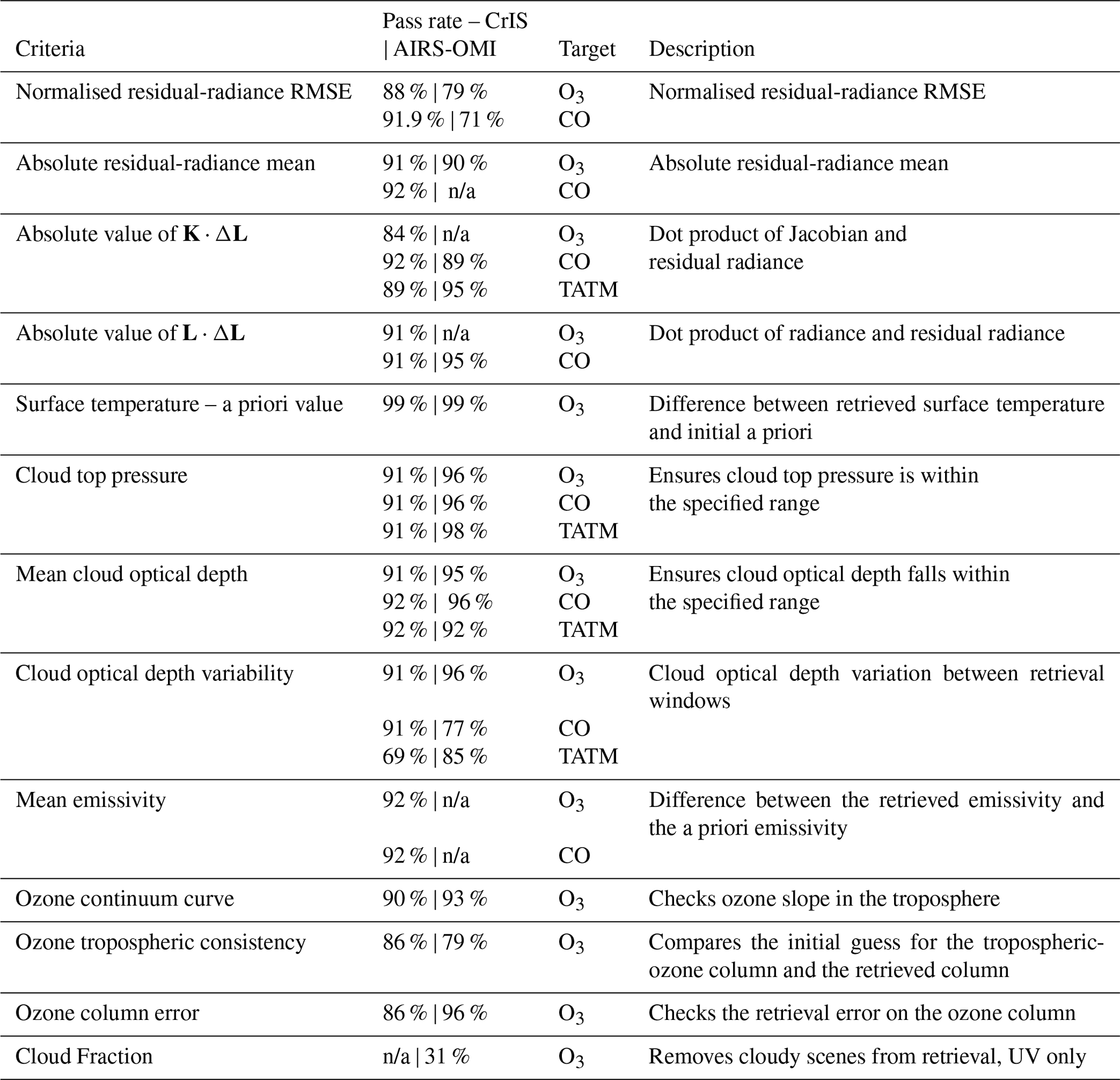
The values shown in Table 4 indicate similar pass thresholds for all of the flags indicated, with some exceptions. For all three targets, the K⋅ΔL flag generally causes the highest failure rates. Here, K is the retrieval Jacobian matrix, i.e. a description of the sensitivity of the forward model to changes in the state vector. ΔL is the residual radiance after the retrieval, i.e. the difference between the measured instrument radiance and the final simulated RTM radiance. Low values of K⋅ΔL indicate that little information remains in the signal, which will occur in challenging retrieval conditions (e.g. high latitudes). TATM retrievals show lower pass rates for cloud optical depth variability compared to other cloud factors. For ozone only, the lowest pass rate flags are the tropospheric consistency and, most significantly, the cloud fraction, which is a factor that is important only in the UV spectral region. The addition of ozone-specific flags indicates that ozone is a highly challenging gas to retrieve, especially in the troposphere where the dynamics of ozone are still poorly understood (Szopa et al., 2021).

Higher failure rates for ozone and TATM for CrIS, as shown in Table 3, compared to carbon monoxide can be attributed to the additional flags shown in Table. 4, except in the case of AIRS-OMI ozone, where the majority of failures are due to the cloud fraction flag. The targets described in this paper are retrieved in serial steps using the same spectrum. However, a poor-quality retrieval from one target will not necessarily impact the other targets.

3.1.1 Training data resampling and dimensionality reduction

We split the dataset, composed of 40 000 individual retrievals, into a training set, which contains 80 % of samples, and a test set, containing the remaining 20 %. In order to avoid biases relating to specific days, we combined the data from all 5 d and ensured even distributions in the training and test sets.

The data are moderately imbalanced since, for example, in the case of CrIS, only approximately 25 % of ozone examples represent failures, while the opposite is true for AIRS-OMI. An uneven representation of classes often poses problems for classification algorithms. A common approach to dealing with unbalanced datasets is to resample the training data so as to simulate a balanced dataset. The simplest methods of balancing the dataset are random undersampling, where we randomly drop a portion of negative (majority class) examples, and random oversampling, where we duplicate a number of copies of positive (minority class) examples so that the portion of positive examples is close to 50 %. We have also considered the more advanced oversampling method, the synthetic minority oversampling technique (SMOTE), where synthetic examples are created as a convex combination of a random positive example and one of its k nearest neighbours (Chawla et al., 2002). Finally, we also considered a combination of oversampling and undersampling, as implemented in SMOTE.

The inputs for classification are spectral data with variable resolutions. We use principal component analysis (PCA) to evaluate whether or not reduced dimensionality of the input spectral data improves the ML pipeline. PCA is a linear method of dimensionality reduction that finds a lower-dimensional representation of the data so that the explained variance is maximised.

3.1.2 The ML model

No single machine learning method is the best choice for every task. Furthermore, different data pre-processing approaches can have a large impact on the ability of models to learn from the data. We refer to a sequence of pre-processing steps and ML models as an ML pipeline.

In order to identify the most appropriate ML pipeline for predicting retrieval failure, we employed the tree-based pipeline optimisation tool (TPOT). TPOT is an automated ML method that optimises ML pipelines using genetic programming (Olson et al., 2016). TPOT makes use of the Python scikit-learn library (Pedregosa et al., 2011) and constructs pipelines composed of the numerous ML tools available (e.g. neural networks, Gaussian processes). For each pipeline, TPOT optimises the hyper-parameters of all of its components. TPOT uses internal cross-validation to optimise hyper-parameters and to evaluate the performance of each pipeline. We choose the pipeline with the best performance in terms of internal cross-validation as the best pipeline for our task and evaluate its generalisation performance based on the so-far untouched test set.

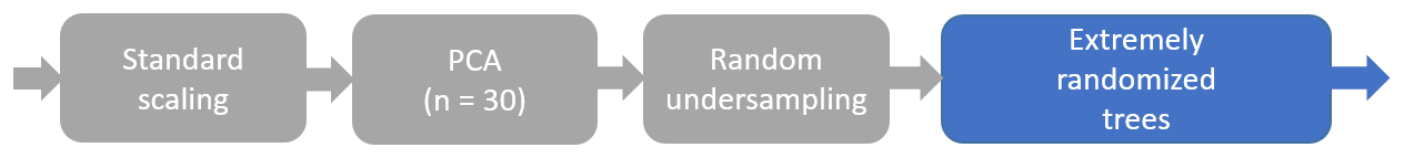
The best pipeline for the task of predicting retrieval failures as identified by TPOT was composed of only one element: extremely randomised trees. We added three pre-processing steps to form the pipeline, as shown in Fig. 2.

• 1. Standard scaling. We apply the transformation $\frac{X_i-{\mathit{\mu }}_{x_i}}{{\mathit{\sigma }}_{X_i}}$, where i denotes the ith input dimension (wavelength), and μ and σ represent the mean and standard deviation, respectively.

• 2. PCA. We perform PCA to reduce the number of dimensions to 30 or to the dimensionality of the dataset, whichever is lower. A total of 30 principal components account for 98.9 %–99.6 % of the explained variance for the full spectrum and 99.99 % of the explained variance for the fitting spectral regions. However, note that we have found mixed results when using the PCA transformation. Sometimes the application of PCA improves the predictive performance of the models, and sometimes reduced performance is observed. Therefore, in Sect. 4, we provide results for when PCA has been applied and for when it has not.

• 3. Random undersampling. Since the failed retrievals are underrepresented in the data, we balance the dataset by randomly subsampling the majority class. Undersampling is used only during training and is skipped during model evaluation and operational use.

• 4. Extremely randomised trees (Geurts et al., 2006). We employ an ensemble learning technique that constructs a large number of decision tree classifiers, i.e. tree-structured models with class labels in leaves and descriptive features in branches. At each branch of a tree, only a restricted subset of features is considered. Both the subset of features and the cut point choice for each feature are randomised. Samples are classified by a majority vote among the classifications of individual trees. The relative importance of each feature can be estimated based on its total contribution to the decrease in class impurity in the nodes of each tree, averaged over the ensemble. In our experiments, we used the scikit-learn implementation of extremely randomised trees, with 100 trees in the ensemble; no depth limitation; and Gini impurity as the measure of split quality, requiring at least two samples to split a node and at least one sample in leaf nodes. The rest of the hyperparameters were left at their default values.

The model takes an L1B spectrum as input and predicts the probability that the trace gas retrieval for that spectrum will result in failure. A discriminatory threshold can then be applied to this output probability in order to make a definitive statement on whether or not a pass or fail is predicted. The assumed threshold is 50 % but can easily be changed in the model depending on the requirements of the user.

Figure 2 Flow chart describing the ML pipeline for the failure prediction model.

Figure 3 Block diagram describing the processing pipeline (the grey boxes) used in the ML model employed in this study and the ML model chosen by TPOT (the blue box). This figure is an in-depth view of the failure prediction model shown in Fig. 2.

4 ML performance assessment

An example of how passed and failed retrievals are distributed globally is shown in Fig. 4. We note a number of regions for both TATM and ozone where failure is common, including northern and southern Africa, as well as parts of China. This figure is for reference; as stated previously, the training and validation datasets are drawn from all 5 d to avoid bias on a particular day.

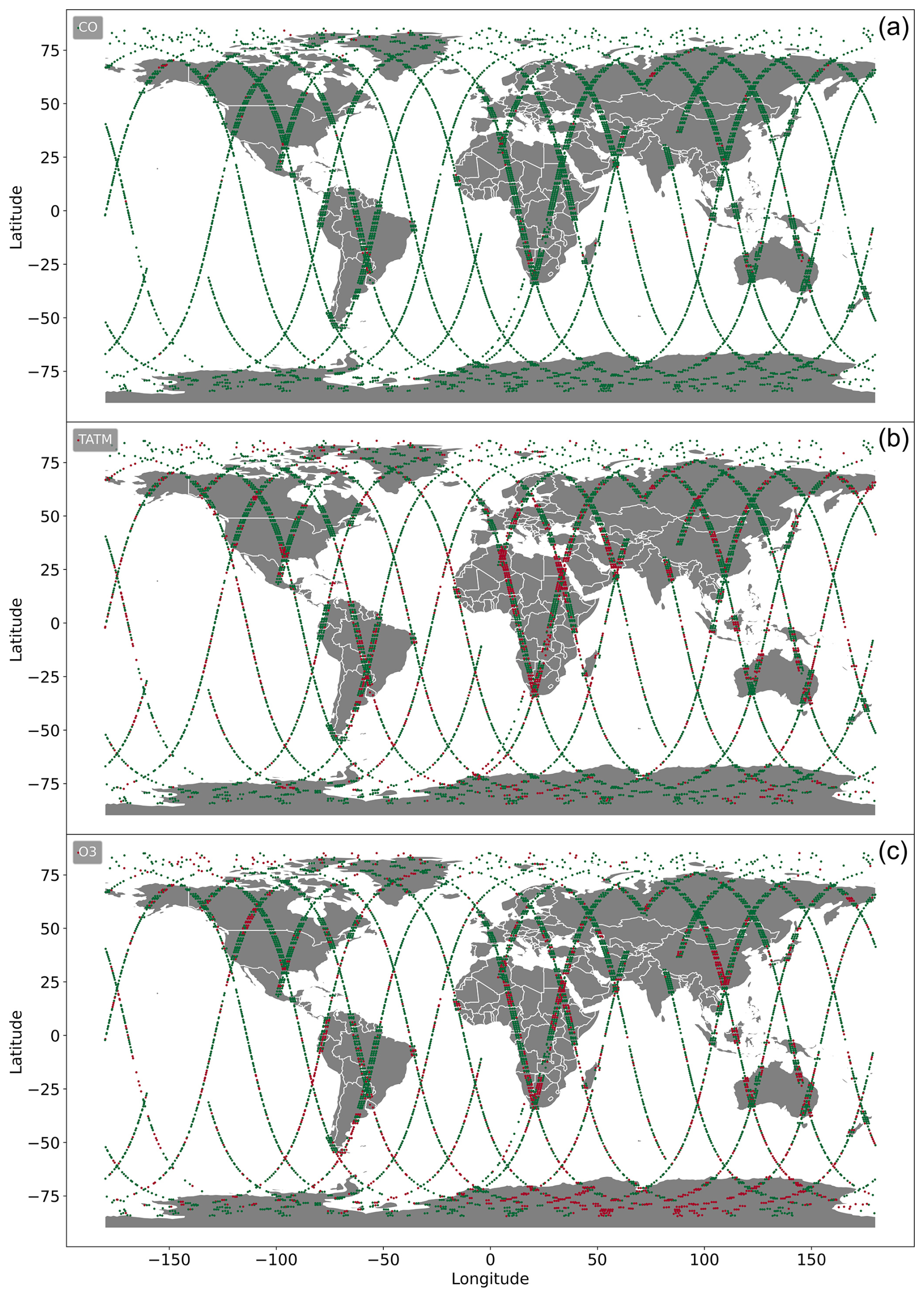
Figure 4 Global distributions of failed retrievals on 15 January 2020 for MUSES CrIS carbon monoxide (a), temperature (b), and ozone (c) profile retrievals. Green markers indicate passed retrievals, and red markers show failed retrievals.

4.1 Receiver operator characteristics (ROCs)

For binary classification tasks, common forms of model assessment are receiver operator characteristic (ROC) curves (Fawcett, 2006). ROC curves compare how many correct positive results are predicted amongst all of the positive samples available (in this case, failed retrievals) against how many incorrect positive results occur amongst all the negative samples (passed retrievals). ROC curves demonstrate the ability of a binary classifier model as its discrimination threshold is varied (as described in Sect. 3.1.2). ROC curves for each of the nine training datasets described in Table 3 are shown to assess the effectiveness of the ML model in each case. The horizontal axis of each graph represents the false-positive rate (FPR) $\mathrm{FPR}=\frac{\mathrm{FP}}{N}$, where FP is the number of false-positive predictions, and N is the number of all negative examples in the test set. The vertical axis shows the true-positive rate (TPR), with $\mathrm{TPR}=\frac{\mathrm{TP}}{N}$, where TP is the number of true-positive predictions, and N is the number of all positive examples in the test set. A perfect model, when represented by an ROC curve, would show all FPR values equal to a TPR of 1.0. The overall performance of the models can be quantitatively described using the area-under-ROC-curve metric (AUC; Flach et al., 2011). AUC is calculated through numerical integration of the ROC curve and is an effective measure of the probability that a failure will be correctly predicted against the probability that a passed retrieval will be classified as a failure without committing to a specific discrimination threshold. An AUC value of 0.5 indicates an uninformed model, with any value above 0.5 showing some benefit to the trained model.

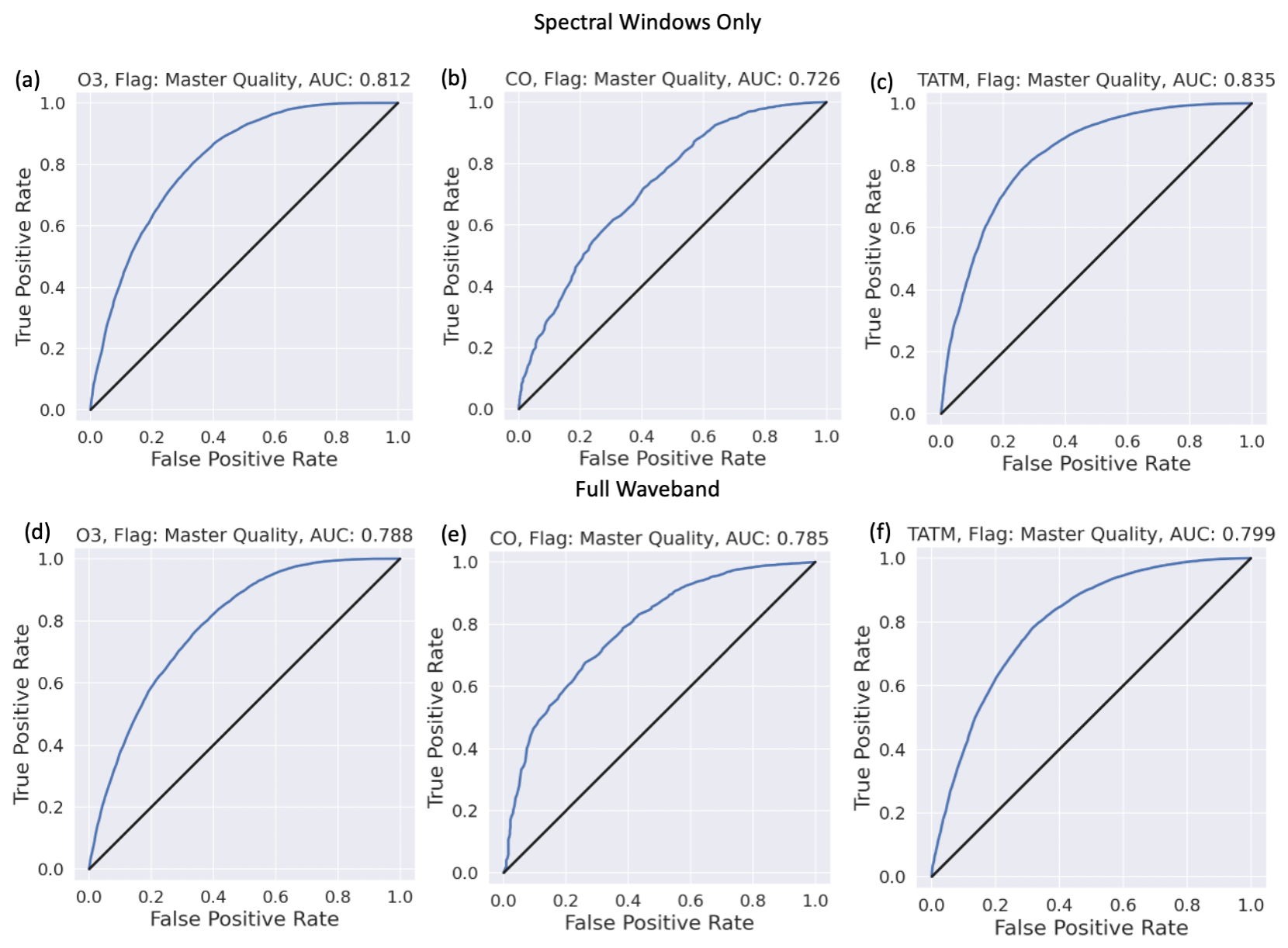
Figure 5 ROC curves for training scenarios 1–6, with the target quantities of ozone, carbon monoxide, and TATM (from left to right) from CrIS input into the ML model having been passed through a PCA. Panels (a)–(c) show ROC curves when the ML tool is trained only on the spectral windows identified in Tables A1, A3, and  A4. Panels (d)–(f) present ROC curves for when the ML tool is trained on the full CrIS spectral range. The blue lines represent the ROC curve for a specific model, while the black 1:1 line represents an uninformed classifier model. The title for each panel indicates the target trace gas, as well as the AUC score for the target and/or window case.

Figure 6 As in Fig. 5 but showing results for the ML model without PCA.

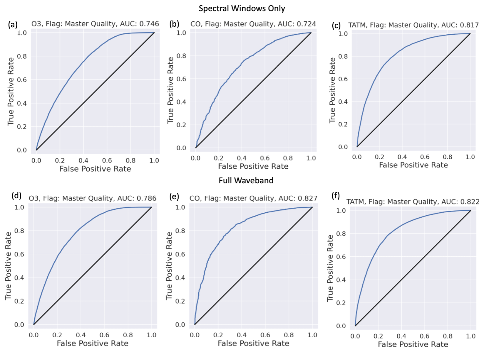
Figure 5 focuses on the results obtained when using PCA in the ML pipeline. The top row of Fig. 5 indicates the clear positive benefit of the models when using only the spectral windows of the relevant trace gases. Both ozone and TATM show superior performance over CO, most likely because of the short spectral window of CO. Both ozone and TATM suggest that the benefit will come from a low threshold value since a high TPR can be achieved with a low FPR; for example, for ozone in panel a, a TPR of 0.5 equals an FPR of 0.1, while a TPR of 0.8 equals an FPR of 0.3. The second row of Fig. 5 indicates the performance of the models when trained on the whole CrIS spectral range. In the case of ozone and TATM, it is not beneficial to use the entirety of the CrIS spectral range, as indicated by the AUC scores in Fig. 5. However, CO shows an 18 % increase in the AUC score when the entire CrIS spectral range is used, most likely due to the short CO spectral window. The use of PCA in the ML pipeline is identified in Fig. 6. The whole CrIS spectral range yields the best AUC scores for each of the trace gas cases.

The AUC scores for all PCA and non-PCA cases are shown in Table 5 for comparison purposes. Table 5 shows that the best results for ozone and TATM are obtained when training is performed only on the relevant spectral windows when PCA is included in the ML pipeline. For CO, the best results are for the ML pipeline without PCA and when the ML model is trained on the whole CrIS spectral band. The results show that there is no “one solution” for the best ML pipeline for trace gas retrieval failure prediction. This is highlighted by the differences in performance between PCA and non-PCA, with window-only ozone showing an 8.5 % AUC score difference, while the equivalent case for TATM only shows a 2 % AUC difference.

Table 5 AUC values for the training datasets.

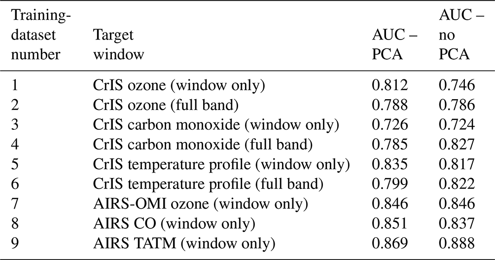
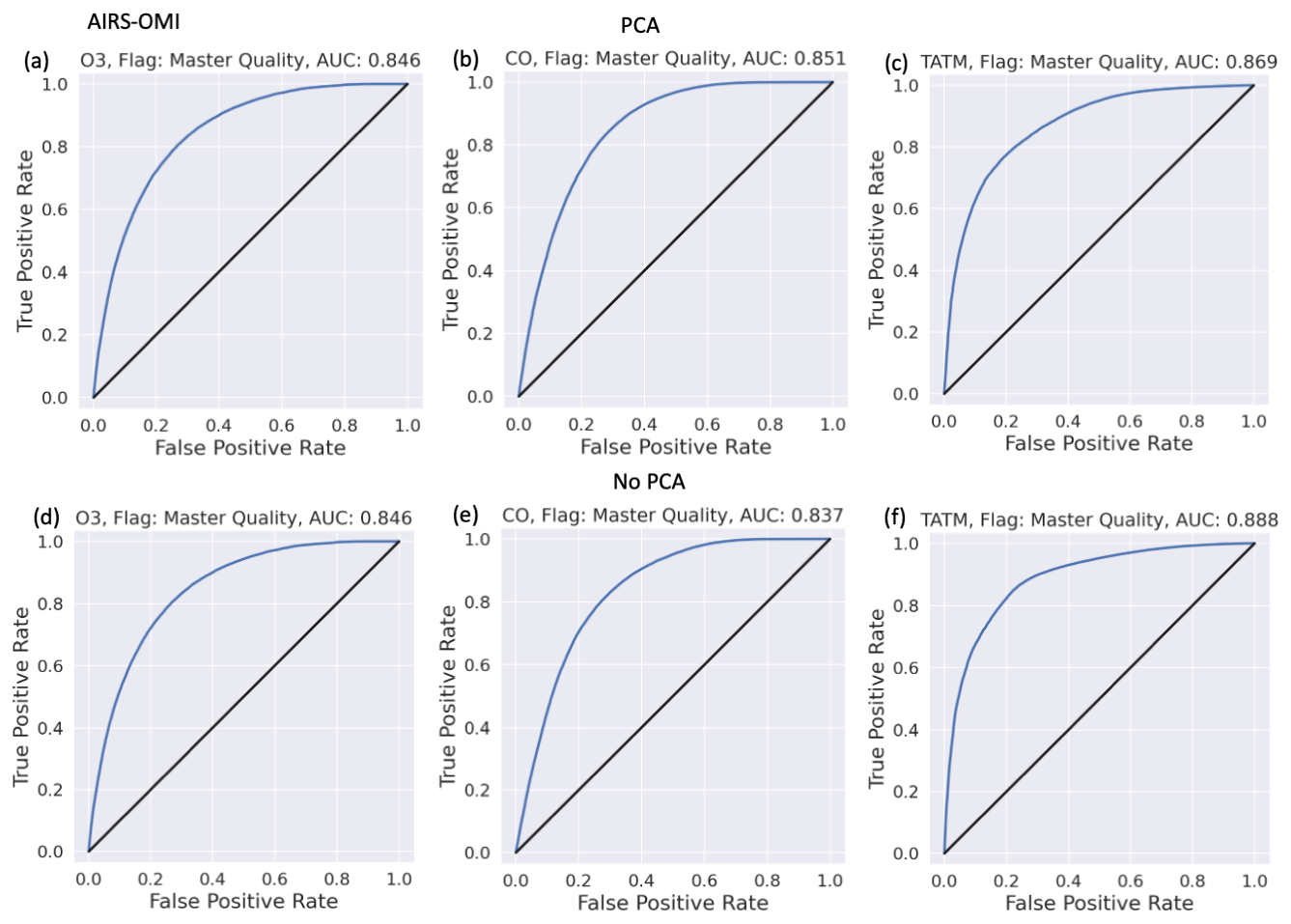
Figure 7 shows the impact of different instruments and wavelengths on the ML models. The AUC values indicate a substantial improvement in comparison to the CrIS results. For example, the results of the equivalent ozone spectral window show a 4 % difference. In particular, the CO windows show improvement despite the use of the same spectral window in both instruments. The use of the PCA or non-PCA case has a limited impact on the AUC scores, suggesting that the use of PCA in the ML pipeline is not important for AIRS-OMI.

Figure 7 ROC curves for training scenarios 7–8; all figure aspects are as in Fig. 5 but showing AIRS-OMI ML results for both the PCA and non-PCA cases.

4.2 Feature importance

Section 4.1 shows that spectral data outside of the CrIS spectral windows indicated in Tables A1, A3, and A4 have an influence on the performance of the failure prediction models, especially when PCA is not used. Here, we investigate if it is possible to determine which wavelengths have a significant influence on the failure prediction models. The extremely random tree classifier easily provides estimations of the relative importance of features, a measure of the likelihood of misclassification caused by that feature (Geurts et al., 2006; Petković et al., 2020). For cases where PCA is used, the input into the classifier is features transformed by PCA, meaning that we multiply each feature importance by its PCA loading coefficient and sum over all the principal components in order to get a feature importance estimate for features in the space of wavelengths. Given the possible impact of the PCA on the performance of the ML models, feature importance was calculated for both PCA and non-PCA cases. The estimates of the importance of the features are shown in Fig. 8. Given that the AIRS-OMI analysis is based on the spectral windows only, AIRS-OMI is not assessed in this section.

The results shown in Fig. 8 indicate limited differences between the target ML models in the PCA cases, suggesting that the PCAs of each of the ML models focus on similar frequencies. The feature importance for the PCA cases shows that spectral regions far outside of the highlighted spectral windows have a significant impact on the ML model performance. For example, in the case of both ozone and TATM, features more than 2 times larger in magnitude are apparent in the SW region of the CrIS spectrum, while neither ozone nor TATM has spectral windows in this region. Note that there are other regions of significant importance outside of the defined spectral windows: below 750 cm⁻¹ (for ozone and CO) and between 1500–1750 cm⁻¹. Considering the non-PCA cases, larger deviations between feature importance in the ML models are apparent. For example, the CO case shows significant importance in the SW band, far in excess of the CO spectral window, which is not apparent in the PCA case. However, the TATM case generally shows importance in the same spectral region as the TATM spectral windows while also exhibiting some importance outside of the fit windows. Note that there remain similarities between the PCA and non-PCA cases, for example, <750 cm⁻¹. These results suggest the necessity of further investigation into non-fitted elements in the retrieval process as these may be having an impact on the overall quality of retrievals and could potentially hint at some of the underlying reasons behind retrieval failure.

4.3 Multiple-flag performance

The results indicated thus far give clear quantitative evidence that predicting poor-quality retrievals with CrIS and AIRS-OMI is feasible. However, these results are based on training on a single master quality flag, which is based on numerous different factors. Some of these factors may have more influence over the master quality flag than others. This means that, even with the feature importance identified in Fig. 8, it is challenging to determine the causes of the failures. Therefore, it is important to identify whether similar results can be obtained by training on the individual quality flags identified in Table 4 and if the influence of these flags can be traced to a specific spectral region. Some of the constituent parts of the master flag may not contribute significantly, and, therefore, training on the individual flags could result in improved performance. Therefore, we performed the same analysis as described previously based on each of the relevant flags.

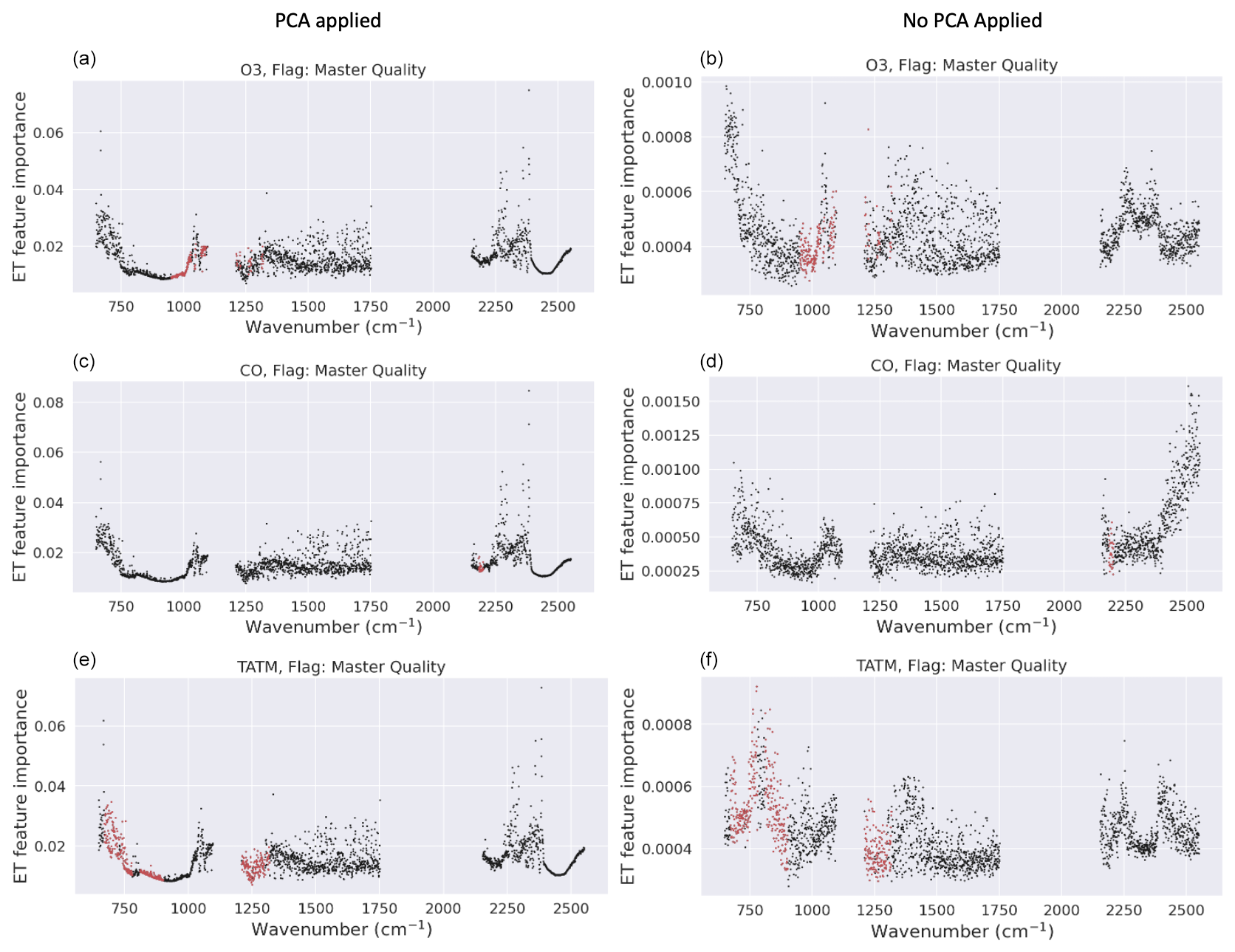
Figure 8 Feature importance of the CrIS full-band models. Panels (a), (c), and (e) show results for the models including PCA(top to bottom: ozone, CO, and TATM). Panels (b), (d), and (f) show the results for the models without PCA, with the same target ordering in rows. The red dots indicate the spectral windows of the retrievals depending on the trace gas, and the black dots indicate wavelengths outside of the spectral windows.

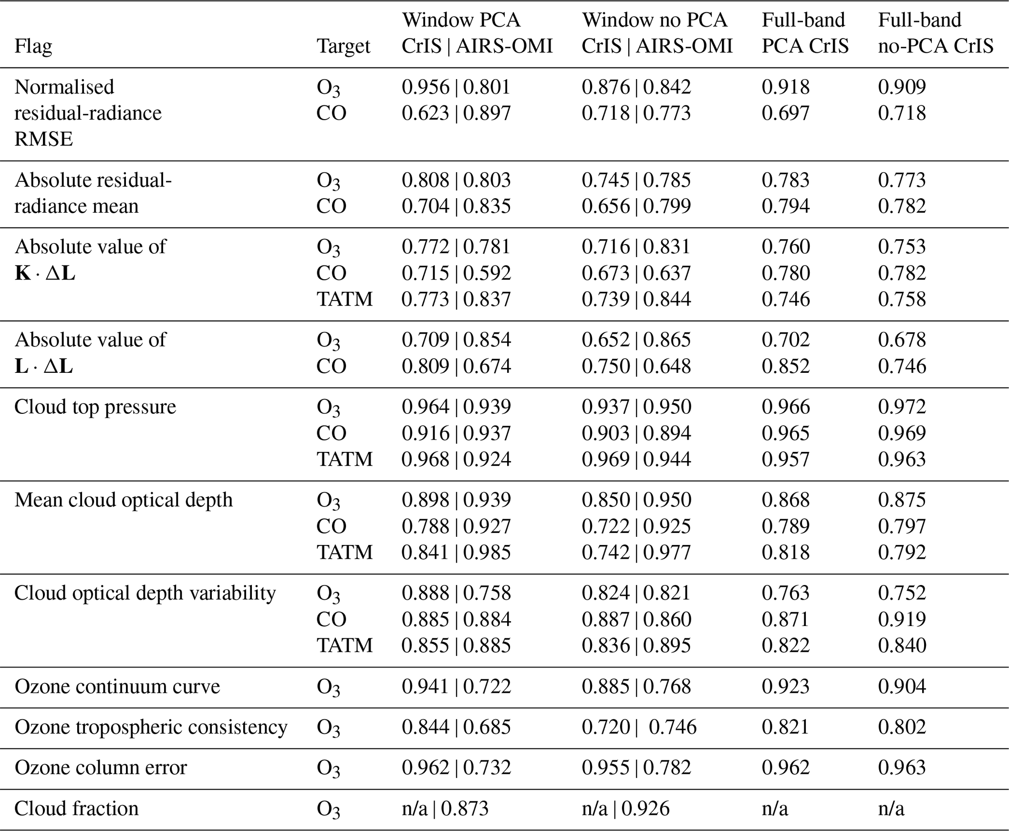
Table 6 AUC values for each of the quality flags identified in Table 4. Training procedure is the same as identified in Figs. 2 and 3. AUC values are shown with PCA both applied and not applied for both the CrIS and AIRS-OMI cases.

The difference between the retrieved surface temperature and the initial a priori surface temperature was not found to be a useful predictor and, therefore, was not included in this analysis.

For CrIS AUC values, the results shown in Table 6 show a pattern similar to those shown in Table 5; that is, typically, the model trained on the spectral window using PCAs yields the best results. There are some exceptions to this; notably, the ML model trained with the full band without PCA has the best performance in the cloud top pressure case for ozone and CO. As with the master quality flag, the training methods (e.g. PCA or non-PCA) have different impacts depending on the quality flag. For example, the ozone tropospheric consistency flag shows a 15 % difference in AUC value between PCA and non-PCA cases (when only using the spectral window). On the other hand, the ozone column error flag shows only a maximum 0.7 % difference between PCA and non-PCA cases. This is also true between targets for the same failure flag – for example, mean cloud optical depth: when ozone is the target, there is a 5.5 % difference between training methods, while, for TATM, there is a 12.5 % difference. This is less surprising given the differences in the quality range for this flag, as identified in Table 4.

In general, training on the individual quality flags yields improved results compared to training on the master quality flags, with the cloud top pressure and ozone column error yielding AUC scores of nearly 1 for the window PCA case. Therefore, this suggests that the ML models can accurately predict failures in those cases. However, there are some cases where the ML models do not perform as well as the master quality flags, for example, for the absolute value of L⋅ΔL. There are multiple reasons for this poorer performance, for example, L⋅ΔL and K⋅ΔL may be challenging for the ML models to effectively learn, or the quality ranges defined in Table 4 could be insufficient, requiring further tuning. We note that K⋅ΔL has the largest failure rate in Table 4, which, logically, would mean that the ML model should have more information about these flag failures as opposed to others, yet the AUC scores suggest otherwise. However, we note that other flags (e.g. ozone column error) also have high failure rates but better ML model performance, meaning that failure rates are unlikely to be influencing the ML model performance. In the case of CO, the ML models are challenged by normalised residual-radiance RMSE and the absolute residual-radiance mean, most likely due to the extremely short CO spectral window (Table A3).

Figure 8 showed the importance of different spectral regions in relation to the master quality flags for CrIS retrievals, and Fig. 9 shows the same analysis for each of the individual quality flags. In this case, we are not investigating the PCA-based ML model results since these show the same patterns as Fig. 8, i.e. importance at the same spectral locations, independent of the flag. It is important to identify that, for most cases, the best ML model results are achieved by a combination of PCA in the ML pipeline and training on the spectral window only (at least in the case of ozone). However, in the following analysis, we aim to identify any potential influence of spectral regions outside of the immediate spectral windows. Such information may influence future spectral-window choices and may indicate how the whole measurement may affect retrieval failures.

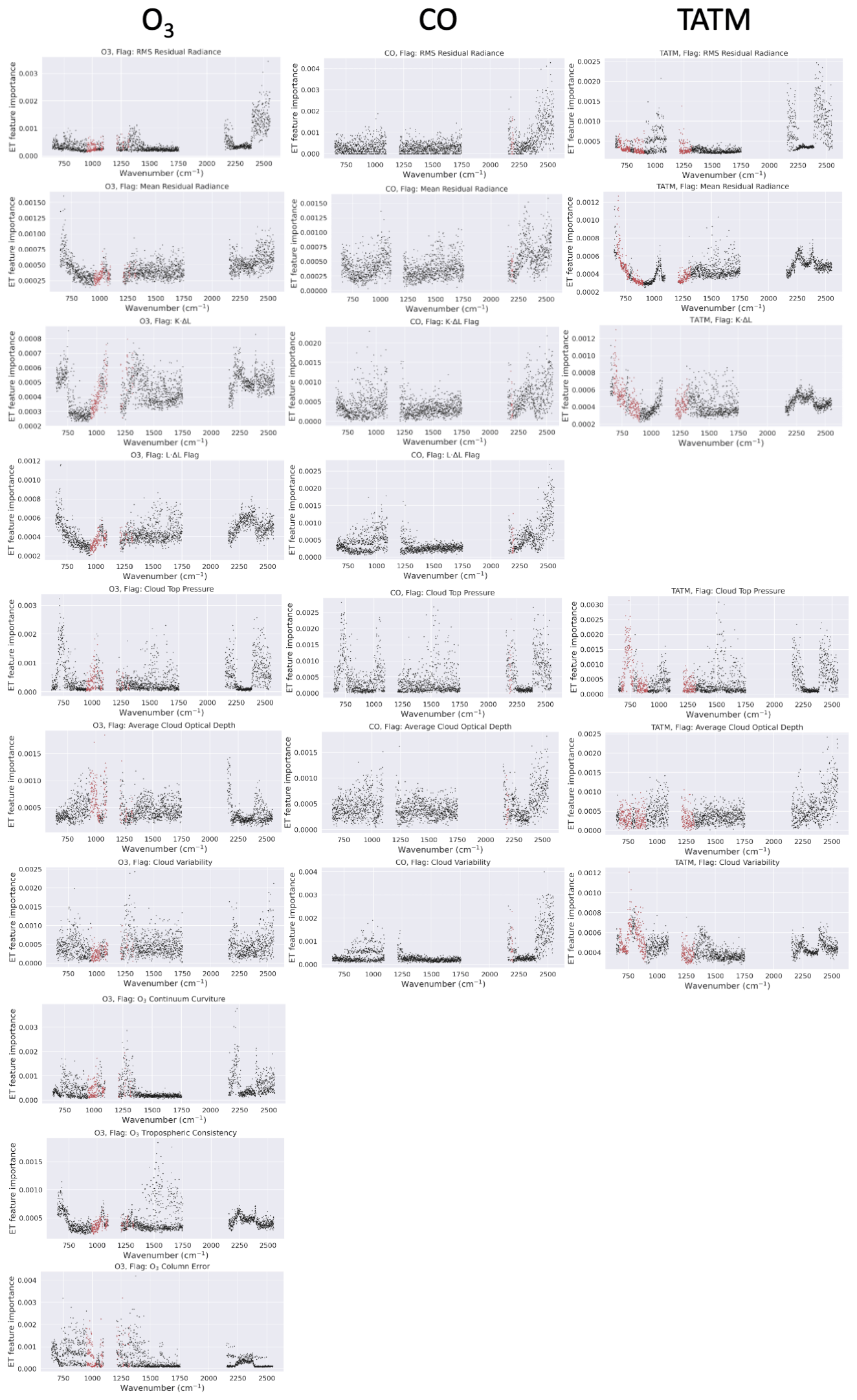
Figure 9 Feature importance for each of the individual quality flags based on an ML model not including PCA, trained on the full CrIS band. The left-hand column shows results for ozone, the middle column shows results for CO, and the right-hand column shows results for TATM. Each row refers to a different flag, as identified in the panel title. Gaps in the panels indicate where a flag is not used for the relevant target. The spectral window of the target is highlighted in red in each panel.

The residual-radiance RMS flag feature importance results are shown in row 1 of Fig. 9; there is a clear dependence on the CrIS SW for all three targets, with the spectral windows for all three targets appearing to be relatively unimportant. Similarly to the master quality flag, failures due to RMS residual radiance could be caused by a number of factors, e.g. clouds in the light path or poor estimation of scattering. This means that attributing RMS failures to specific causes will be difficult. The CrIS retrieval pipeline includes the retrieval of cloud top pressure and extinction, including spectral windows in the SW, meaning that it may be possible to attribute this sensitivity to cloud-related failures. Note that the feature importance plots for cloud top pressure (row 5) and average cloud optical depth show similar behaviours in the SW. Focusing on mean residual radiance in row 2, for ozone and TATM, importance features are evident in the LW, matching some of the spectral windows of TATM, implying that the mean residual radiance for ozone is dependent on TATM. Conversely, in the SW, CO and TATM show similar features, suggesting a CO dependence on TATM in the SW. The feature importance for K⋅ΔL (row 3) in the case of CO and TATM is very similar to the equivalent plots for mean residual radiance. Indeed, the AUC values in Table 6 are very similar for CO, implying that these quality flags draw information from the same spectral regions. However, there is less similarity in ozone, where far more importance is attributed to the micro-windows in the LW and MW. However, significant importance is still apparent in the SW, again suggesting that ozone absorption outside of the CrIS MUSES micro-windows can impact the quality criteria. The importance of features with the L⋅ΔL flag is shown in row 4, with only ozone and CO using this flag. The ozone micro-windows do not show significant features and are similar to the results shown for the mean residual radiance, implying that the whole CrIS spectral range contributes to this failure flag. This is contrasted by the feature importance for CO, where the LW and MW have lower levels of importance when compared to the SW.

The cloud top pressure flag in row 5 shows similar features for all three targets, with notable features at 750, 1000, 1500, 2100, and 2400 cm⁻¹. Cloud top pressure is one of the few flags that shows the best performance when trained on the whole spectral range, which is highlighted by the fact that the feature importance plots are almost identical across the targets. Note that the allowable range for Cloud top pressure is identical for all three targets. Row 6 shows the features for average cloud optical depth; again, there are similarities between the CO and TATM features, with the maximum importance toward the shorter end of the SW. Ozone, while having similar features compared to CO and TATM in the LW and MW, shows unique characteristics in the SW. Here, both CO and TATM have identical quality criteria for average cloud optical depth, while ozone has a much more stringent requirement. Note that the ozone windows in the LW indicate significant importance, which is supported by the AUC values in Table 6, where there is limited difference in the AUC values despite the learning method, implying that cloud optical depth is best described by the ozone windows in the LW. Row 7 shows the feature importance of cloud variability; in this example, each of the targets exhibits very different behaviour. For ozone, the feature importance is largely equivalent across the whole spectrum, suggesting that no information is gained outside of the ozone spectral window, which is supported by the AUC values. For CO, there is significant importance shown in the short end of the SW, similarly to cloud top pressure. The AUC values in Table 6 for CO suggest that there is improved ML model performance when using the whole available spectral band, suggesting that additional CO windows not used in the MUSES retrievals are possible. For TATM, there is little variation between the bands, and the AUC values do not indicate significant differences between the learning methods, thus implying that there is nothing to learn from the wider spectral bands. The final three flags in rows 8, 9, and 10 are only relevant to ozone. For ozone continuum curvature, the feature importance is similar to that of CO with cloud variability. In general, there is low feature importance; however, the SW which has no ozone windows indicates two spectral regions where importance is larger than any other feature. The MW channel generally shows no importance, except where the ozone micro-windows are found, while the LW channel shows importance across the whole band. For the ozone tropospheric consistency flag in row 9, limited importance is attached to the ozone micro-windows, with the largest features occurring toward the shorter end of the MW and the longer end of the LW. Finally, the ozone column error is investigated in row 10; note that, as shown in Table 6, the AUC values for each learning method are very similar, suggesting that the importance is largely confined to the ozone micro-windows. The feature importance plot largely supports this result, with the majority of the features being confined to the ozone micro-windows or the surrounding spectral regions.

As with the feature importance plots for the master quality flags shown in Fig. 8, it is not possible to identify one spectral region as the cause of flag failures. However, in some cases, it is more obvious than in others; for example, flags such as RMS residual radiance are dependent on numerous effects, while ozone column error is restrained to certain spectral regions. There is some indication in these results that this type of feature analysis could be used to further refine spectral windows for trace gas retrievals. Further, the SW CrIS band, despite having limited use in the MUSES CrIS retrievals (CO and a cloud micro-window), seems to have significant importance across most of the failure flags. Further investigation into why this is the case is required.

5 Statistical analysis using independent dataset

The previous subsections have quantified the performance of the ML models; however, in practice, a threshold value must be chosen in order to apply the ML models. Here, we analyse the statistical significance of the ML model predictions by relating the binary predictions to the true-failure flags output from the MUSES algorithm using independent CrIS and AIRS-OMI datasets not used to train the ML models, in this case, roughly 40 000 retrievals from 12 August 2020. Figures 10 and 11 compare MUSES failure flags with the percentage probability of failure predicted by the ML model trained using PCA based on the spectral windows alone.

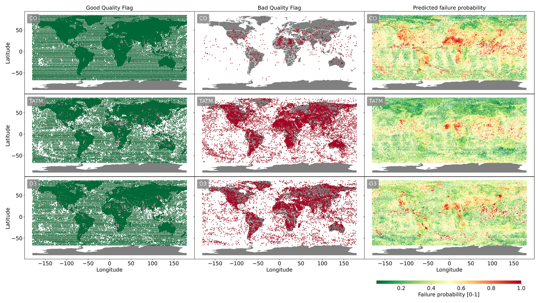
Figure 10 Quality flags from MUSES CrIS retrievals of CO, TATM, and O₃ on 12 August 2020, where the left-hand column (green) indicates triggering of the good-quality flag, and the middle column (red) indicates the triggering of bad-quality flags. Predicted probability of failure [0–1] from ML models for CO, TATM, and O₃ (the rows) on the same day can be seen in the right-hand column

What is clear from the analysis of CrIS and AIRS-OMI data in Figs. 10 and 11 is that the ML models are capable of predicting the actual failures. However, in the locations surrounding the failure positions, the ML models often predict a high probability of failure, reducing the performance of the model, meaning that the choice of the threshold will have a significant impact on the use of the ML models.

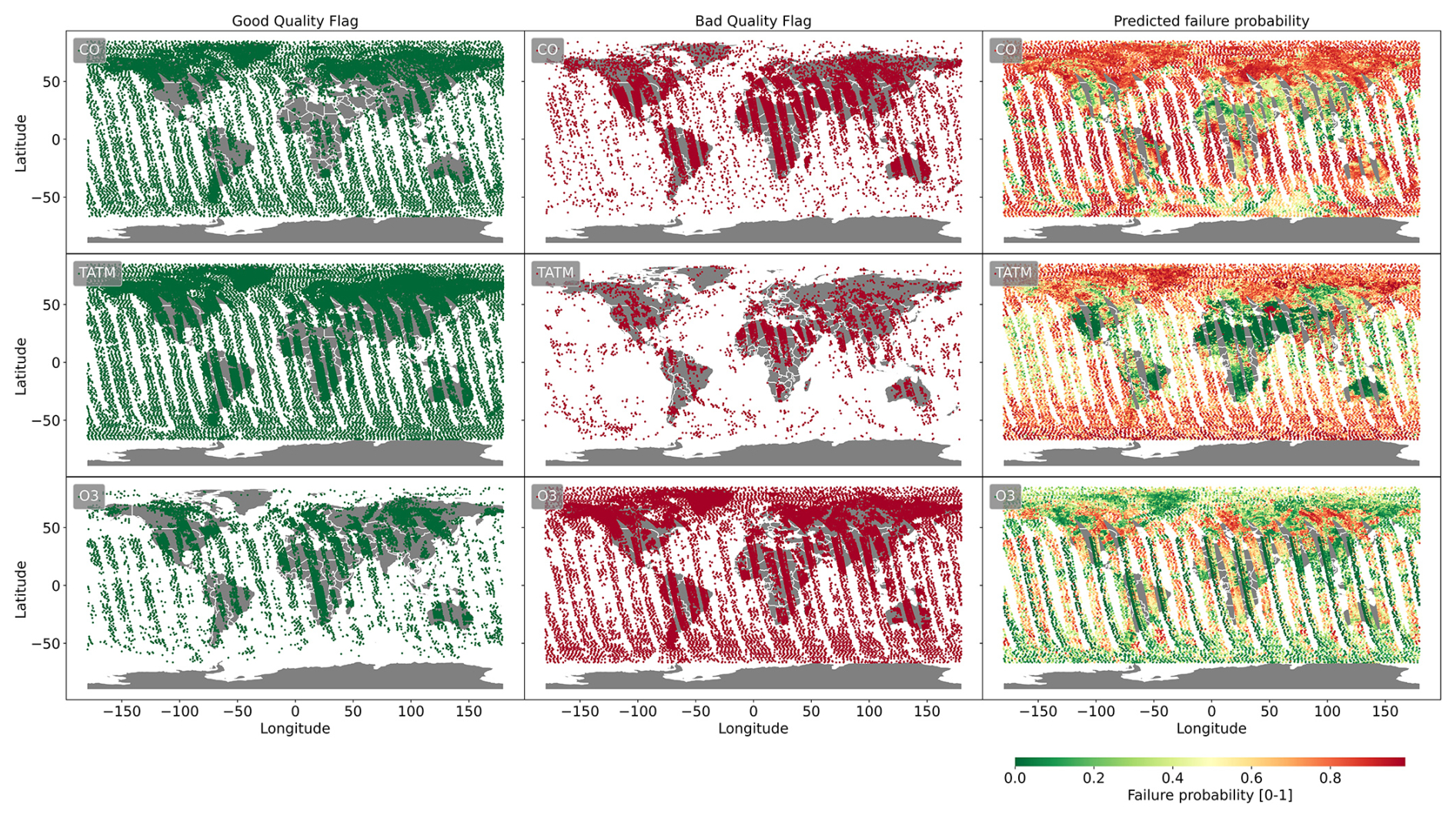
Figure 11 As in Fig. 10 but for AIRS-OMI retrievals.

To assess the importance of this threshold, we use Cramér's V metric to assess how strongly two categorical variables (in this case, the reported MUSES failure flag and the ML-model-predicted failures) are associated. With this analysis, we can understand if there is any statistical significance between what the ML models predict as failures and the truth. Cramér's V metric is defined as follows:

$$\begin{array}{}\text{(1)}& V={\displaystyle \frac{\sqrt{\frac{{\mathit{\chi }}^{\mathrm{2}}}{n}}}{\mathrm{DOF}}},\end{array}$$

where χ is the chi-square statistic, n is the total sample size, and DOF is the degrees of freedom of the signal of the dataset. A value of 0 for V means that there is no association, and 1 means perfect association; however, the interpretation of the degree of association depends on the DOF, which, in this study, are equal to 1. In this case, we assume that a small association is 0.1 ≤ V<0.3, a medium association is 0.3 ≤ V<0.5, and a large association is V≥0.5.

Figure 12 indicates the Cramér's V metric for the CrIS dataset for each quality flag for the three target quantities for a range of ML model thresholds. Both ozone and CO show peak importance at the threshold value of 0.6 while also showing a steady increase in importance between thresholds of 0.1 to 0.6. The reasons why ozone and CO have a maximum association at 0.6 while the TATM association is at 0.4 are unclear, but this is most likely due to the different quality criteria. Note that each quality flag for CO shows similar importance values at each threshold, while TATM and ozone show more variation. For example, the master quality flag and ozone column error show the strongest associations, even at high thresholds, unlike any of the remaining quality flags. This is an interesting result, given that Table 6 shows numerous ozone quality flags as having AUC values similar to the ozone column error.

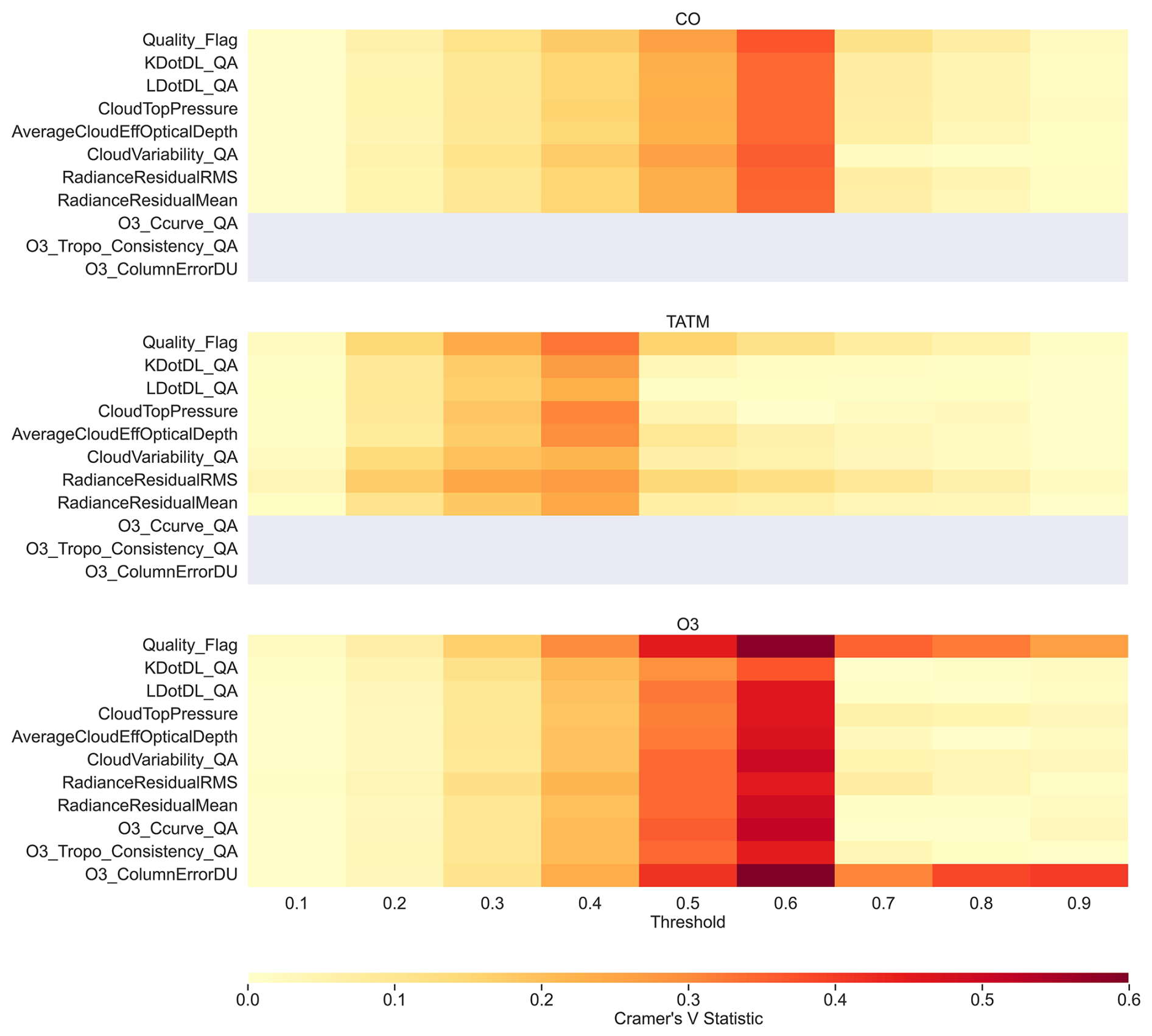
Figure 12 Cramér's V statistics for the CrIS dataset between quality flags and the independent predicted dataset for varying thresholds of pass of failure, ranging from 0.1 to 0.9, for the three gases: CO, TATM, and O₃. A small association is defined by values of 0.1–0.3, a medium association is defined by values of 0.3–0.5, and a large association is defined by values of >0.5.

Figure 13 displays the Cramér's V metric for the AIRS-OMI dataset for each quality flag for the three target quantities for a range of ML model thresholds. Both TATM and CO show slightly higher importance for the quality flag above other flags, with medium associations at 0.2–0.3. For CO, peak importance is achieved at a threshold of 0.8, and that for TATM remains relatively constant in terms of the threshold but with a peak at 0.9. All other flags for CO reach peak importance at a threshold of 0.5. For TATM, associations are small, ranging from 0.1 to 0.3, and show no clear pattern between flags or thresholds. The only exception is CloudVariability_QA, which has a higher importance at low thresholds. Ozone flags show the strongest associations compared to TATM and CO. In particular, the Quality_Flag, RadianceResidualRMS, and OMI_CloudFraction flags display the strongest associations above 0.5. In the case of the latter flag, importance is constant in terms of the threshold (always greater than 0.6), indicating that cloud fraction is a critical quality flag despite the prediction threshold. All other flags show decreasing importance with increasing thresholds, starting with relatively high associations at 0.5.

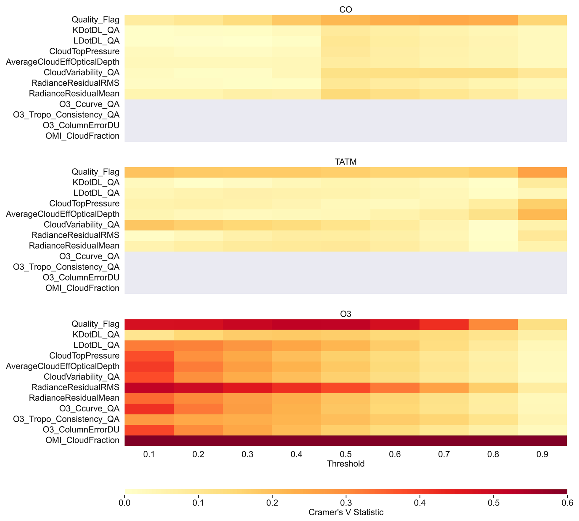
Figure 13 Cramér's V statistics for the AIRS-OMI dataset between quality flags and the independent predicted dataset for varying thresholds of pass or failure, ranging from 0.1 to 0.9, for the three gases: CO, TATM, and O₃. A small association is defined by values of 0.1–0.3, a medium association is defined by values of 0.3–0.5, and a large association is defined by values of >0.5.

Figure 14 shows the result of applying the ML filtering technique using threshold values of 0.5 and 0.2 to the MUSES CrIS retrieval pipeline for ozone. The CrIS-retrieved ozone concentrations are at an exemplar pressure level (681 hPa) and are split into daytime and nighttime. The top panels show the retrievals without quality-controlling or ML filtering to act as a baseline, where a total of 39 892 retrievals are available. The middle panels show the CrIS retrievals with MUSES quality-controlling applied, where a pass rate of 73 % is found. The panels second from the bottom indicate MUSES retrievals with ML filtering at a threshold 0.5 and with quality-controlling applied, where, after filtering, 28 085 retrievals are available, with a pass rate of 85 %. The bottom panels indicate a filtering threshold of 0.2 (i.e. retrievals with a probability of failure of 0.8 or above are removed). In this case, 37 683 retrievals are available, with a pass rate of 77 %. Once adjusted for quality, the non-ML case has 29 121 good-quality retrievals, the case with an ML threshold of 0.5 has 23 872, and the case with a threshold of 0.2 has 29 015. These results show a clear indication of the impact of the ML model. For the 0.5 threshold case, the ML model removes 35 % of the retrievals in the standard pipeline. In the case with a threshold of 0.2, 6 % of the retrievals are removed whilst retaining a similar number of good-quality retrievals compared to the non-ML case.

In the case with a threshold of 0.5, the removal of 35 % of the retrievals is a huge gain; however, there is a cost, namely a 20 % loss in good-quality retrievals. This loss is obvious in Fig. 14, with clear patterns in terms of the filtered retrievals. The majority are removed from the Sahara Desert, the Arabian Peninsula, central Asia, and the western United States. The retrievals that have been removed are typically on the extreme end of magnitude, especially over central Asia. We note that, when quality-controlling is applied to the CrIS retrievals, it is largely the high-concentration values that are removed, implying that high-ozone-concentration retrievals in the troposphere are more likely to be of poor quality, and this is likely the reason why the ML model classifies high ozone concentrations as more likely to fail. The mean ozone concentration for the non-quality-controlled case is 47 ppb, that for the quality-controlled case is 46 ppb, and that for the case with a threshold of 0.6 is 45 ppb. For the case with a threshold of 0.2, using the TROPESS processing system, roughly 3 h of processing were saved, which will vary depending on the processing system. However, over larger time periods, such time saving will mount up quickly.

This challenge of failures over desert regions requires additional analysis; it is possible that more effective results will be obtained by training an ML model with only data obtained over deserts, suggesting that regional ML models may be more effective than global models.

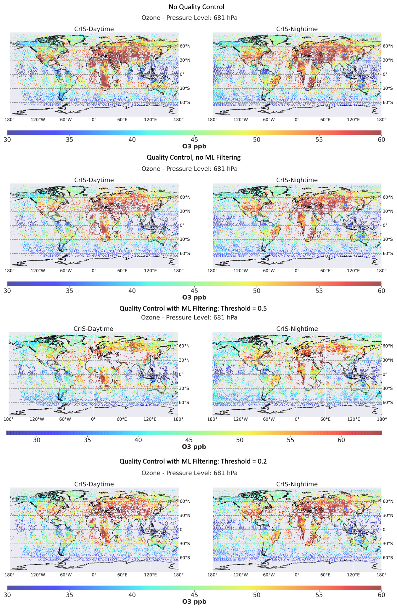
Figure 14 Impact of applying the ML filter to MUSES ozone retrievals. The top panels show CrIS daytime and nighttime retrievals at the 681 hPa pressure level using the standard MUSES processing with no quality-controlling. The middle panels are as above, but standard quality-controlling flags are applied. The bottom panels show the same data when the ML filter is applied with a threshold of 0.5 and 0.2, with the remaining data having been quality-controlled.

Figure 15 presents the results of applying an ML-filtering technique using threshold values of 0.5 and 0.2 to the MUSES AIRS-OMI retrieval pipeline, as with the CrIS case for ozone. The top-left panel shows the retrievals without quality-controlling or ML filtering to act as a baseline, where a total of 24 382 retrievals are available. The top-right panel shows the AIRS-OMI retrievals with MUSES quality-controlling applied, where 8026 good-quality retrievals are available, indicating a pass rate of 33 %. The bottom-left panel indicates MUSES retrievals with ML filtering at a threshold 0.5 and with quality-controlling applied, where 6386 good-quality retrievals are available, meaning that the ML filtering captures 80 % of the good-quality retrievals. The bottom-right panel indicates a filtering threshold of 0.2. In this case, 7850 good-quality retrievals are available, meaning that the ML filtering captures 98 % of the good-quality retrievals. These results show a clear indication of the impact of the ML model. For the case with a threshold of 0.5, the ML model removes 74 % of the retrievals in the standard pipeline. In the case with a threshold of 0.2, 68 % of the retrievals are removed. Unlike in the CrIS case, for AIRS-OMI, Fig. 15 shows that the ML filtering does not target and remove specific geographical regions, indicating that the cloud filtering works very well.

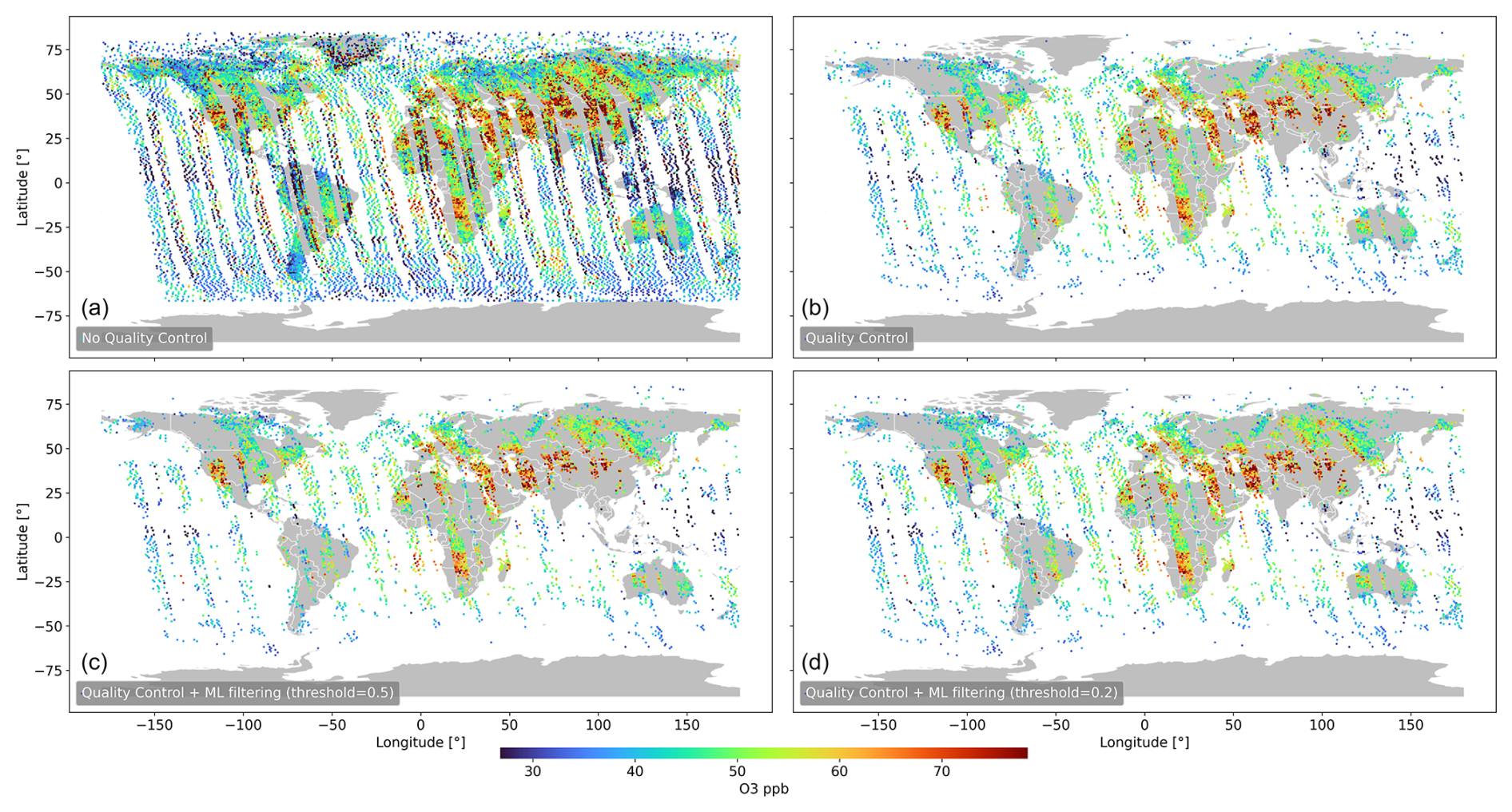
Figure 15 Impact of applying the ML filter to MUSES ozone retrievals for AIRS-OMI. Daytime retrievals at 681 hPa pressure level using the standard MUSES processing with no quality-controlling (a) and with standard quality-controlling flags applied (b). The ML filter is applied with thresholds of 0.5 (c) and 0.2 (d), with the remaining data having been quality-controlled.

6 Discussion

One of the primary metrics used in this paper, AUC, is an efficient way to assess model performance. However, a choice must be made when implementing a failure prediction model in a retrieval pipeline. For example, models should be employed carefully, i.e. setting the failure threshold value high and only removing retrievals that have a very high probability of failure, but a significant percentage of retrievals that will fail through the pipeline should be allowed. Alternatively, should no caution be used, the failure threshold should be set low, with the removal of almost all of the failed retrievals but also with the removal of large volumes of good-quality retrievals. There are arguments to be made for both positions; however, currently, it is not practically possible to process the millions of satellite measurements and convert them into L2 trace gas concentrations in real time. Therefore, if having as much real-time data as possible is desired, the most logical solution will be to use a low threshold, therefore removing most of the available data from the retrieval pipeline but guaranteeing a high likelihood that all processed retrievals will be of good quality.

The threshold values lead to a further point of contention: the MUSES CrIS and AIRS-OMI retrieval pipelines simultaneously retrieve CO and ozone, as well as several other trace gases. There will be cases where the ozone retrieval will fail while other products may not or vice versa. In this case, a decision must be made as to whether or not to ignore all trace gas retrievals from a particular spectrum or to keep those that do pass the initial failure check.

There is a significant cost–benefit aspect to the ML model, where significant processing speed-ups can be achieved while potentially valuable information may be lost. At this time, the ML models are sufficiently developed to be deployed in an operational sense, especially with a low threshold value, which incurs minimal risk of the loss of valuable retrievals. However, there are clearly more improvements that could be made; for example, the cost–benefit might be improved with a greater amount of and/or more sophisticated training of the ML model, potentially to the point where there is very little cost in applying the ML model, which is a topic for further work and exploitation. For example, training could be undertaken per region rather than globally, which may yield improved results. Further, more work can be performed on the quality-assured (QA) values that the ML models are trained on. These are currently applied globally, but there could be some value in deriving QA values for distinct regions and training the ML model on these regions.

As an alternative to regional models, the training data could be carefully constructed to ensure a similar frequency of retrieval failures geographically. Variations across time (night and day, different seasons, cloud coverage, etc.) could be balanced in a similar fashion. In terms of ML, the classification performance may be improved by considering more classification methods and, particularly, more elaborate methods of dimensionality reduction that might be more suitable for spectral data.

In general, training is key to the effectiveness of ML models. Numerous training datasets were applied, including much denser sampling of CrIS retrievals, yielding dataset sizes of 100 000 or more retrievals. However, in general, we found minimal impact with regard to both AUC scores and experiments, similarly to Fig. 14. This highlights a challenge given the difficulty experienced by the ozone ML model over desert regions, indicating that blindly training with larger datasets will not solve the problem. Some ways to address this would be taking into account the fail rate of different regions when preparing the training dataset or taking into account geographical location when performing over- or under-sampling.

As satellite instruments age, the quality of the spectral radiances can degrade. For example, in the case of OMI, the quality of some OMI pixels has limited the latitudinal range of the instrument (Levelt et al., 2018), while, in the case of the Suomi NPP CrIS, failures in the longwave channels of the “side-2” electronics suite in May 2021 forced a switch to “side-1” electronics in order to retain the use of the LW channels (Iturbide-Sanchez et al., 2021). The implication is that, as instruments age and decay, the ML models will need to be re-trained to account for any degradation.

One of the implications of this paper is that ML models can differentiate different atmospheric conditions from measured spectra. This implies that an appropriately trained ML model may be able to infer trace gas concentrations directly from measured spectra as opposed to using the OEM or other retrieval methods, similarly to the work conducted by Van Damme et al. (2017) and Loyola et al. (2020). While this makes for interesting future work, the risks of all ML methods, such as appropriate training sets and unintended biases, would apply, which would add uncertainties to any retrievals derived from this method.

Finally, as with all ML approaches, there are challenges that could cause some problems with the results. For example, are the training datasets representative or are biases introduced during training (amongst many other common issues not directly identified here)? It is likely that some issues are present in the current form of the ML model presented in this paper (for example, biases). However, in order to increase confidence in the results, we evaluated the performance of our ML model in two stages: first, using cross-validation (a standard and rigorous evaluation procedure in ML) and, later, using a completely new, so-far-unused dataset. The relatively high predictive ability of our models indicates that they are capturing meaningful information and are effective. Therefore, although the performance of the ML models can, most likely, be improved, we are confident that they are effective.

7 Conclusions

The ability of retrieval algorithms to convert satellite spectra into trace gas quantities in a timely manner is a key challenge in the future of EO. Tens of millions of measurements will be generated per day, representing a significant challenge to processing all of these measurements in real time. A significant drain on the processing of these millions of retrievals is the fact that failed retrievals require the same amount of resources as good-quality retrievals, wasting huge amounts of computational effort. In this paper, we provide an ML method for reducing the processing overhead of retrieval algorithms by predicting whether or not a retrieval will fail based on the characteristics of an instrument-measured spectrum prior to performing a full retrieval. This was achieved by training an extremely-randomised-tree ML model on the Suomi NPP CrIS and AIRS-OMI spectra and quality flags from the TROPESS–MUSES algorithm for ozone, carbon monoxide, and temperature profile retrievals. We show a test case focusing on ozone, where, from a pipeline of 37 683 CrIS retrieval targets, applying the ML filter prior to full retrieval removes 13 811 targets. Of the 13 811 targets, ∼ 20 % were misclassified, which could be reduced given more targeted training regimes. On the other hand, in the case of AIRS-OMI, from a pipeline of 24 382 retrieval targets, the ML filter removes 16 532 targets. Of the 16 532 targets, ∼ 2 % were misclassified, showing a high-quality tool.

The retrieval algorithm quality flags used in this assessment are based on numerous individual flags, designed to catch errors. We show that, in some cases, specific spectral regions can be identified as influencing these flag failures. Focusing on these spectral regions could help identify why retrieval failures occur.

The ML models identified in this paper are based on open-source Python packages which are simple to train and apply, given sufficient training data. This failure prediction model represents a significant contribution toward reducing the processing overheads of current and future EO satellites.

Appendix A: Retrieval windows

The spectral windows for the targets covered in this study for AIRS and CrIS are highlighted in Table A1 for ozone, Table A3 for carbon monoxide, and Table A4 for temperature profile. For the OMI ozone window, these can be seen in Table A2. These are graphically represented in Fig. 1.

Table A1 MUSES micro-windows used for CrIS and AIRS ozone retrievals.

Table A2 MUSES micro-windows used for OMI ozone retrievals.

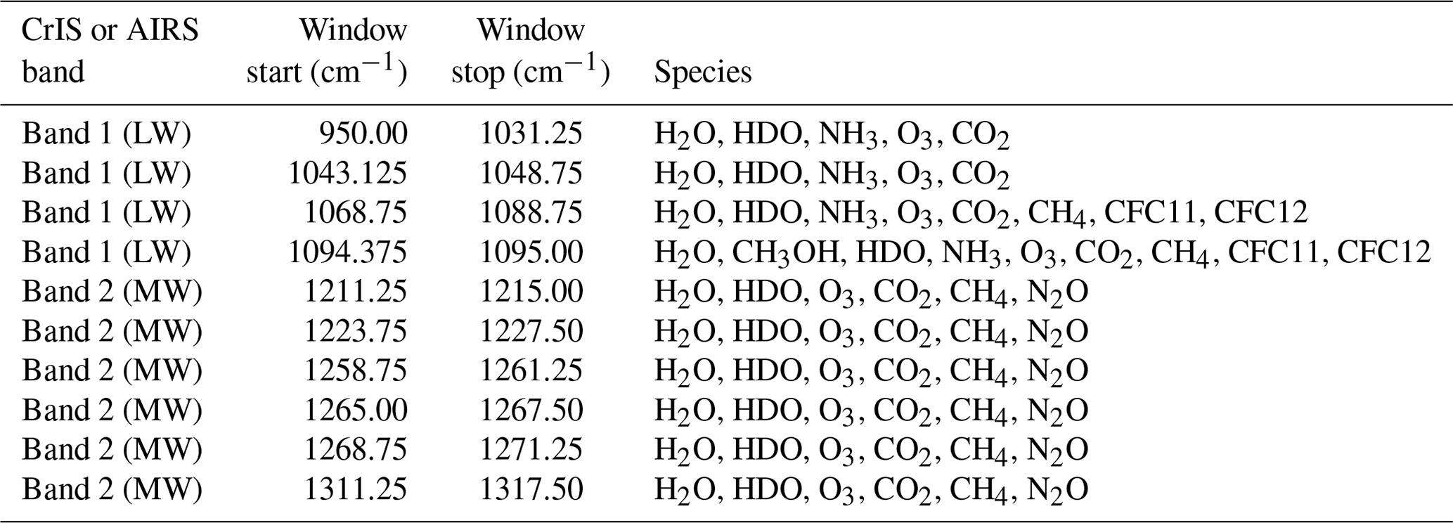
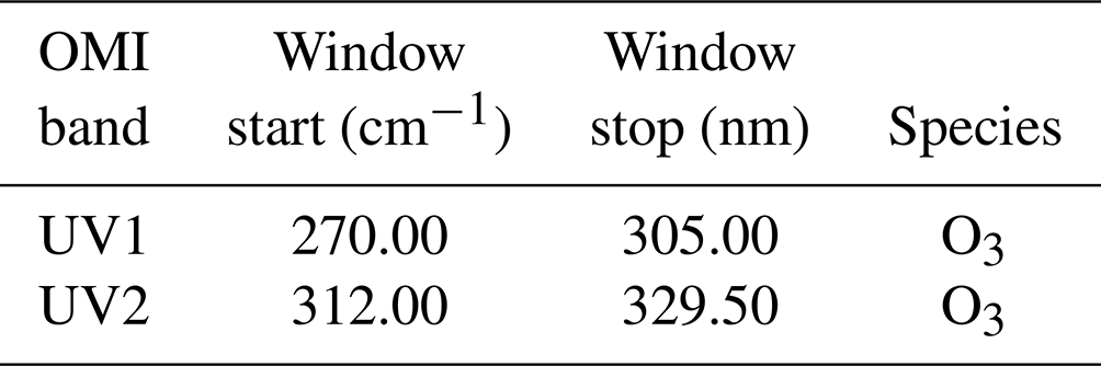
Table A3 MUSES micro-windows used for CrIS or AIRS carbon monoxide retrievals.

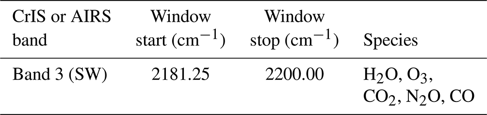
Table A4 MUSES micro-windows used for CrIS or AIRS temperature profile retrievals.