Radar-based high-resolution ensemble precipitation analyses over the French Alps

Reliable estimation of precipitation fields at high resolution is a key issue for snow cover modelling in mountainous areas, where the density of precipitation networks is far too low to capture the complex variability of these fields with topography. Adequate quantification of the remaining uncertainty in precipitation estimates is also necessary for further assimilation of complementary snow observations in snow models. Radar observations provide spatialised estimates of precipitation with high spatial and temporal resolution and are often combined with rain gauge observations to improve the accuracy of the estimate. However, radar measurements suffer from significant shortcomings in mountainous areas (in particular, unrealistic spatial patterns due to ground clutter, leading to local systematic biases). Precipitation fields simulated by high-resolution numerical weather prediction (NWP) models provide an alternative estimate but suffer from widespread systematic biases and positioning errors. Even though these uncertainties can be partially described by ensemble NWP systems and systematic errors can be reduced by statistical post-processing, NWP precipitation estimates are still not reliable enough for the requirements of high-resolution snow cover modelling.

In this study, better precipitation estimates are obtained through a specific analysis based on a combination of all these available products. First, a pre-processing step is proposed to mitigate the main deficiencies of precipitation estimates by radar and gauges, focusing on reducing unrealistic spatial patterns. This method also provides a spatialised estimate of the associated error in mountainous areas, based on a climatological analysis of both radar and NWP-estimated precipitation. Three ensemble daily precipitation analysis methods are then proposed, first using only the modified precipitation estimates and associated errors, then combining them with ensemble NWP simulations based on the particle filter and ensemble Kalman filter data assimilation algorithms. The performance of the different precipitation analysis methods is evaluated at a local scale using independent ski-resort precipitation observations. The evaluation of the pre-processing step shows its ability to remove the main spatial artefacts coming from the radar measurements and to improve the precipitation estimates at the local scale. The local-scale evaluations of the ensemble analyses do not demonstrate an additional benefit of ensemble NWP forecasts, but their contrasted spatial patterns are challenging to evaluate with the available data.

1 Introduction

Monitoring snow cover in mountainous areas is essential for a wide range of practical applications and scientific applications (IPCC, 2022). The complex topography of these areas leads to a very high spatial variability of meteorological and snow conditions (e.g. Clark et al., 2011), which is not fully sampled by any existing in situ observing network, especially at high altitudes (Thornton et al., 2022). Operational applications such as water resource management or avalanche forecasting, which require detailed monitoring of meteorological conditions and snow cover over large mountainous areas, suffer from this lack of observational information. The use of numerical snow models provides more continuous spatial and temporal coverage than observations. The complexity of such models varies widely depending on their application (Krinner et al., 2018). However, all seasonal snow modelling systems are affected by the strong dependence of the snow cover state at any time on its past evolution since the first snowfall. This long-term dependence means that any simulation error at any time can affect all subsequent simulations, resulting in an accumulation of errors throughout the winter.

Satellite observations of some snow properties provide a great opportunity to identify and reduce these errors (Awasthi and Varade, 2021; Largeron et al., 2020). Methods based on ensemble data assimilation algorithms have been developed to process these observations (Magnusson et al., 2017; Cluzet et al., 2021). According to Cluzet et al. (2022) and Deschamps-Berger et al. (2022), these methods primarily use snow observations to compensate for errors in the precipitation forcing of the snow cover model. Quantifying the uncertainties in the precipitation fields is therefore essential to fully benefit from the assimilation of snow observations. However, all the papers cited above rely only on stochastic perturbations of the precipitation dataset, obtained with homogeneous and rather arbitrary error estimates in the absence of more advanced quantification of precipitation uncertainty.

Existing snow cover modelling systems mostly use precipitation inputs provided by numerical weather prediction (NWP) output, surface observations, or a combination of these two sources of information (Morin et al., 2020). Surface observations provide reliable local estimates of precipitation but are affected by systematic undercatch in the case of solid precipitation or in windy conditions (Rasmussen et al., 2012; Kochendorfer et al., 2020). In addition, the under-sampling of higher elevations (Thornton et al., 2022) means that there is a lack of information on the spatial distribution of elevation-dependent variables, such as precipitation (Mott et al., 2023). On the contrary, high-resolution NWP models produce spatialised estimates of precipitation fields at different spatio-temporal resolutions. Lundquist et al. (2019) argue that such models can simulate annual precipitation accumulation in mountainous areas better than estimates from gauge- or radar-based observations. However, they suffer from biases and positioning errors in individual events and in seasonal accumulations. These errors are problematic for snow cover modelling (Vionnet et al., 2016, 2019; Haddjeri et al., 2023). A combination of surface observations and NWP output is used in some operational snow modelling systems (SAFRAN; Durand et al., 1993; Lespinas et al., 2015) to provide precipitation estimates at scales of a few hundred square kilometres. However, scarce observations may be insufficient to constrain high-resolution precipitation analyses in mountainous areas (Soci et al., 2016), even when specifically designed for this purpose (Schirmer and Jamieson, 2015).

Radar measurements provide high-resolution spatial estimates of precipitation. However, they are subject to uncertainties in mountainous regions, mainly due to the interaction between the radar beam and the terrain (ground clutter and partial masks) (Germann et al., 2022; Foresti et al., 2018; Faure et al., 2019; Yu et al., 2018; Foehn et al., 2018; Ghaemi et al., 2023). Methods have been developed to correct radar-based precipitation fields (Vogl et al., 2012) and to assess the associated uncertainty (Kirstetter et al., 2010, 2015; Villarini et al., 2014). The combination of radar measurements and in situ observations of precipitation (Sideris et al., 2014; Sivasubramaniam et al., 2019; Champeaux et al., 2009) does not fully mitigate these uncertainties, as in situ measurements generally do not sample areas where these uncertainties are the most significant. More sophisticated products combining NWP outputs, surface observations, and precipitation estimates from radar measurements (CaPA; Fortin et al., 2015, 2018; Khedhaouiria et al., 2022) suffer from significant biases in winter (Lespinas et al., 2015). The potential of using radar observations for detailed snowpack modelling has only been investigated on a relatively large scale over the French Alps (Birman et al., 2017). Over the Austrian Alps, the SNOWGRID system (Olefs et al., 2013) uses radar observations via the INCA now-casting system (Haiden et al., 2011) to force a simple snowpack model designed for hydrological applications. The low quality of precipitation estimates based on radar measurements in complex terrain currently prevents their direct use to successfully force a detailed snowpack model at high spatial resolution (Haddjeri et al., 2023). In particular, the spatial structure of the error associated with such products in mountainous areas and its overall magnitude have not been investigated in depth.

As noted above, Cluzet et al. (2022) and Deschamps-Berger et al. (2022) showed that any precipitation analysis designed for a snow cover modelling system with assimilation of snow observations must include an estimate of the precipitation analysis errors. In particular, snow data assimilation is effective when uncertainties in the precipitation forcing are correctly identified and accounted for, which can be achieved through accurate and reliable ensemble precipitation analysis (Cluzet et al., 2021). In the context of high-resolution modelling, radar-based precipitation analyses present the advantage of providing already spatialised precipitation estimates. A variety of methods have been developed to produce ensembles of estimated precipitation from radar and gauge measurements with varying degrees of complexity (Clark and Slater, 2005; Germann et al., 2009; Mandapaka and Germann, 2010; Dai et al., 2014; Kirstetter et al., 2015; Frei and Isotta, 2019). However, they were not designed to meet the requirements of snow data assimilation in a high-resolution snowpack modelling system. Ensemble methods combining radar-based precipitation estimates and NWP output are more common in the now-casting context (Foresti et al., 2012; Nerini et al., 2019; Atencia et al., 2020a; Sideris et al., 2020). In this case, NWP output is used to propagate the precipitation estimation in time but not to mitigate the inherent flaws in the radar product itself.

To address this gap, the aim of this study is to explore the combination of different products based on radar, gauge, and NWP data (Sect. 2) to produce ensemble precipitation analyses (Sect. 3.2) over mountainous areas. An evaluation of the quality of several available precipitation estimation products is first performed (Sect. 4.1). Then, a pre-processing step of the best product is proposed to remove spatial artefacts. Finally, this study develops three different methods for ensemble analysis of daily precipitation to investigate the benefits of combining observational precipitation estimates and NWP outputs. These methods are then applied to produce ensemble analyses of daily precipitation at a 1 km resolution (see Sect. 3.2). Section 4.2 evaluates their performance, and Sect. 5.3 discusses their respective advantages and disadvantages. This study focuses specifically on the French Alps, but the proposed methodology can be applied to any mountainous area with at least 1 year of radar-based and NWP model precipitation estimates. These analyses are expected to appropriately quantify precipitation uncertainties in order to guarantee the efficiency of the assimilation of snow observations in snow cover simulations.

2 Precipitation dataset

This study focuses on the French Alps region (Fig. 1) for the period from 1 August 2021 to 1 August 2022.

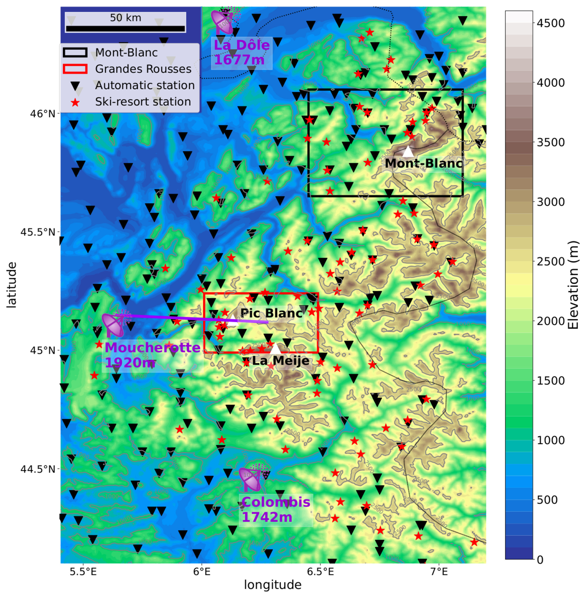
Figure 1 Relief at 250 m resolution of the French Alps domain used in this study, showing the three radars used in radar-based precipitation estimation products, the automatic observation stations, and the reference ski-resort observation stations used for verification. The Grandes Rousses and Mont Blanc areas, on which parts of this study are focused, are framed, and the cross section of Fig. 2 is marked with a grey line.

Three different observational precipitation estimates and one from a high-resolution NWP model were considered. To avoid confusion between snow variables, we follow the international classification for seasonal snow on the ground (Fierz et al., 2009) and express all precipitation in kg m⁻². A 24 h accumulation of all precipitation products up to 08:00 CEWT is analysed in this study.

2.1 Radar product (PANTHERE)

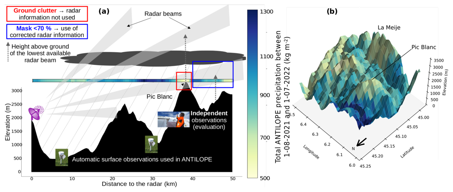
Figure 2 (a) Illustration of radar measurement issues from the Moucherotte radar towards the Pic Blanc in the Grandes Rousses massif (grey line in Fig. 1). Radar beams from four elevation angles are shown to illustrate the vertical sampling of the atmosphere and its limitations in complex terrain. The effect of ground clutter management in the PANTHERE algorithm and the link with the underestimation of precipitation over mountain ridges are illustrated over the Pic Blanc (framed in red). The horizontal coloured band in panel (a) is the ANTILOPE precipitation accumulation on the ground between 1 August 2021 and 1 July 2022 along the transect between the Moucherotte radar, which is the primary contributor to the PANTHERE precipitation estimation in this area, and the Pic Blanc. The positions of two automatic gauges and a ski-resort observation site are also shown to illustrate the altitudes of typical in situ observations used in the ANTILOPE product and the reference observations used in this study, as well as the lack of in situ observations at altitudes above 2000 m. (b) ANTILOPE precipitation accumulation between 1 August 2021 and 1 July 2022 over the relief of the Grandes Rousses domain (framed in red in Fig. 1).

PANTHERE (Tabary, 2007; Figueras i Ventura and Tabary, 2013) is an operational quantitative precipitation estimation (QPE) product based on the combination of most of the French metropolitan radar data. It has a 1 km horizontal resolution and a temporal resolution of 5 min, aggregated in this study into 24 h precipitation accumulations at 08:00 CEWT each day. Each radar measures the reflectivity and dual-polarisation variables with a resolution of 240 m × 0.5°, up to a maximum range of 255 km, and at several elevation angles (see grey radar beams in Fig. 2a). After a correction step to account for measurement problems, the reflectivity Z is converted to an instantaneous precipitation rate R ($\mathrm{kg}{\mathrm{m}}^{-\mathrm{2}}{\mathrm{h}}^{-\mathrm{1}}$) using a Z–R relationship (Marshall and Palmer, 1948) that is constant in space and time. This precipitation rate is then corrected by applying a vertical profile of reflectivity (VPR) correction factor. The purpose of this step is to correct for the expected variation in reflectivity with altitude due to different hydrometeor types and in particular to correct for the increase in reflectivity in the melt region, known as the “bright band”. Although this method is effective in most cases, it has some limitations: it assumes a constant precipitation rate below the bright band, so processes such as evaporation or low-level enhancement of precipitation must be considered (Le Bastard et al., 2019).

After this processing of the volumetric radar data, the precipitation rate at ground level is estimated from a combination of collocated precipitation rates estimated at all heights, weighted by their quality index, which depends on, among other factors, the height of the measurement. The final 5 min QPE at ground level is then obtained by accumulating the precipitation rates over time. In this study, precipitation accumulations over 24 h are considered. Despite all these steps to calculate the QPE, its quality in space is variable. In general, the uncertainty of the estimate increases with the height of the radar beam above the ground, implying that the most valuable radar information comes from the lowest radar heights and that the quality of the precipitation estimate tends to decrease far away from the radar. In particular, Fig. 2a illustrates that stratiform precipitation systems are not detected by radar beams above the top of precipitation clouds.

In mountainous areas, the radar beam will also often intercept the ground. Radar elevations affected by ground clutter are rejected by the algorithm (red frame in Fig. 2), and the lowest information comes from the next beam above, which affects the quality of the precipitation estimate. In addition, the conical shape of the radar beam means that the beam width increases with distance from the radar (up to about 1000 m at a distance of 50 km). It can also be partially affected by the presence of a mountain (blue frame in Fig. 2). In this case, the affected beam information is considered unusable behind the mountain if the mask blocks more than 70 % of the total energy; otherwise the signal is corrected for attenuation.

Faure et al. (2017) evaluated the quality of PANTHERE precipitation estimation over the French Alps and showed an increasing underestimation of precipitation towards the east due to radar beam blockage and increasing distance from radars. They also identified specific areas affected by significant underestimations related to ground clutter handling (as shown in Fig. 2) and concluded that the clutter correction is ineffective in a high-mountain context. Similarly, Faure et al. (2019) studied the vertical distribution of PANTHERE precipitation estimates and highlighted a general overestimation of the radar QPE at the bottom of the valleys and an underestimation at the highest altitudes.

2.2 Radar–gauge combination product: ANTILOPE

ANTILOPE (Champeaux et al., 2009) is an operational composite analysis combining radar precipitation estimates from PANTHERE and precipitation observations from automatic gauges (see Fig. 1). It is available at a 1 km resolution, and 24 h accumulations at 08:00 CEWT have been used in this study. The fusion of these two sources of information is based on a scale separation between small-scale convective and large-scale stratiform precipitation. Precipitation associated with radar-detected convective cells is corrected by a spatialisation of the local differences between radar and gauge precipitation estimates using inverse distance interpolation. Large-scale precipitation is estimated by a spatialisation of the gauge values by an ordinary kriging with external drift method, using either a correlogram computed from radar images or an exponential variogram model if no radar image is available. In contrast to PANTHERE, the quality of ANTILOPE precipitation estimation in mountainous areas is not well documented. The strong dependence of the ANTILOPE product on the radar-based precipitation estimate suggests that the main drawbacks of radar measurements described in Sect. 2.1 also affect the ANTILOPE quality. However, the use of rain-gauge observations may reduce the magnitude of the errors, with possible exceptions in the case of assimilation of non-heated gauges not detected by the control steps.

2.3 Gauge kriging

In order to document the added value of the radar information used in ANTILOPE, a precipitation estimation based on the same kriging method (using an exponential variogram) of the same set of gauges (automatic stations, Fig. 1) as those used in the ANTILOPE algorithm but without any radar information was set up and evaluated for this study. This represents 512 stations across the study area with elevations ranging from 0 to 2730 m a.s.l. and a mean elevation of 809 m a.s.l. The resulting precipitation fields have the same 1 km resolution as the ANTILOPE and PANTHERE products and are used similarly. The temporal resolution used in this study is 24 h. As already mentioned, gauge measurements are known to be affected by significant undercatch in the case of solid precipitation and in windy conditions (Rasmussen et al., 2012; Kochendorfer et al., 2020).

2.4 Numerical weather prediction model

In this study, data from the deterministic NWP model AROME (Seity et al., 2011; Brousseau et al., 2016) and its ensemble version have been used in a complementary way.

The French operational high-resolution NWP model AROME provides hourly precipitation forecasts with a 1 km resolution. Daily precipitation accumulations (liquid and solid) are directly derived from the 24 h forecast at a validity time of 07:00 UTC (08:00 CEWT). Yearly AROME precipitation accumulation is then calculated as the accumulation of daily precipitation between 1 August 2021 and 1 August 2022.

A 16-member ensemble version of the AROME NWP model is also operational at a 2.5 km resolution (Bouttier et al., 2016). Its precipitation forecasts are statistically post-processed with the method developed by Taillardat et al. (2019), based on quantile regression forests, to provide an unbiased and well-distributed ensemble of hourly precipitation forecasts, hereafter referred to as PEAROME. The calibration uses ANTILOPE precipitation estimates as a reference and is performed at two AROME EPS initialisation times (09:00 and 21:00 UTC) with lead times of up to 45 h (Taillardat and Mestre, 2020). Physically realistic precipitation patterns are then reconstructed using the ensemble copula coupling method of Schefzik et al. (2013). However, the training method has been evaluated over mainland France (Taillardat and Mestre, 2020), and its performance over the French Alps is not well known. The daily precipitation used in this study is the precipitation accumulation between lead times of 10 and 34 h from the 21:00 UTC initialisation time. The raw precipitation fields are downscaled to the ANTILOPE 1 km grid by a bi-linear interpolation so that the model and observations can be compared at the same spatial and temporal resolution.

2.5 Evaluation data

The evaluation dataset comes from the observation network of the ski resorts of the French Alps (Fig. 1). These observations are not used by the ANTILOPE product (and therefore not used in gauge kriging). This network provides a set of daily humanmade meteorological and snowpack observations specifically designed for avalanche forecasting during the winter season (generally from mid-December to mid-April, depending on the opening and closing dates of the resorts). For this study, observations of 24 h precipitation accumulation in a bucket weighted at 08:00 CET are used as the reference for all evaluations. Consequently, all precipitation products are evaluated in terms of 24 h water equivalent accumulations starting at 08:00 CET (07:00 UTC in winter, 06:00 UTC in summer). Evaluation data are only available for the period from 1 December 2021 to 30 April 2022. This means that there is a 1 h gap between the precipitation accumulation of the different products (up to 07:00 UTC) and the reference observations (up to 08:00 CET) for the month of April after the time change. However, this gap is expected to have a very limited impact on the results, as fewer reference observations are available in April (due to the closure of ski resorts), and only two significant precipitation events occur during this period. A human estimate of the highest altitude reached by the rain–snow limit during the same period is also available and used in this work. When focusing on solid precipitation, only days when the rain–snow limit altitude was below the station altitude were considered.

Ski-resort observations have limitations for the evaluation of gridded precipitation estimates:

• Human measurement time may vary slightly between stations and days.

• The mountainous environment is known to affect the measurements from the gauges, with possible snow accumulation in the gauges or undercatch in windy conditions (these measurement errors are sometimes detected and corrected or removed in the monitoring process of the observations and also affect the automatic gauges used by the ANTILOPE product).

• Local gauge observations do not have the same representativeness as a gridded estimate over a pixel of about 1 km².

Nevertheless, these are the only available independent data for the evaluation of the various precipitation products.

3 Method

3.1 ANTILOPE observation error

A precipitation analysis requires the specification of the error of the various products involved. As mentioned earlier, radar-based observations are known to suffer from important shortcoming in mountainous areas (Germann et al., 2022). In particular, unrealistic spatial patterns of ANTILOPE yearly precipitation accumulation estimates can be visually identified over some mountain ridges. Figure 2b shows that ANTILOPE yearly precipitation accumulations over the ridges of Pic Blanc and La Meije (around 600 kg m⁻²) are unrealistically low. In comparison, the same accumulation at lower altitudes between the two peaks benefiting from direct gauge measurements is more than twice as large (up to 1300 kg m⁻²). Figure 3a shows the same pattern over the Mont Blanc (circle in red) where yearly precipitation accumulation (less than 200 kg m⁻² per year, 5 times less than in the Chamonix Valley, circle in green) is unrealistically low. These patterns are also visible in the daily precipitation fields (Fig. 5) and are probably due to the presence of ground clutter (see Sect. 2.1).

The most common approach to overcoming the limitations of radar-based precipitation estimates in mountainous areas is to combine them with other sources of information or to apply a calibration step (Germann et al., 2022). However, these methods suffer from the lack of observations at high elevations (Fig. 1). McRoberts and Nielsen-Gammon (2017) proposed a method to detect and correct pixels affected by partial beam blockage based on an analysis of the radar precipitation estimation climatology, but it does not specifically focus on ground clutter, which is prevalent in mountainous areas. Haiden et al. (2011) use radar precipitation estimates where ground clutters have been statistically filtered, and other perturbations are dealt with in a pre-processing step based on a climatological scaling of the radar data. Here, we propose a method to mitigate the unrealistic spatial patterns in ANTILOPE precipitation fields. A first method to estimate the climatological errors in ANTILOPE is described in Sect. 3.1.1, and an evaluation of the method is provided in Sect. 4.2. This estimated climatological error is then used to remove the unrealistic spatial structures in ANTILOPE 24 h precipitation fields (Sect. 3.1.4).

3.1.1 ANTILOPE climatological error estimation

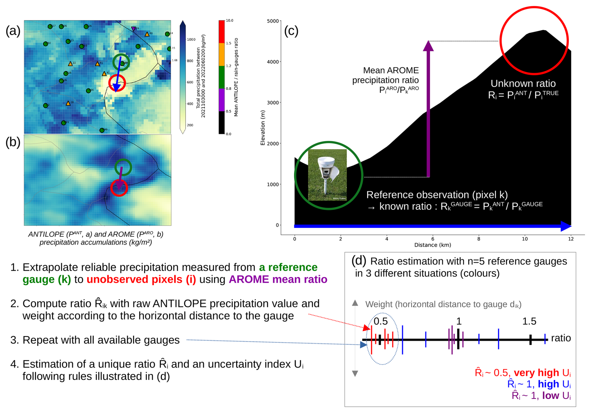
Figure 3 Illustration of the climatological ANTILOPE error estimation over the Mont Blanc (circled in red) based on (a) the yearly ANTILOPE precipitation accumulation (P^ANT) from 30 October 2021 to 2 June 2022 and the mean ANTILOPE$/$gauge ratio (R^GAUGE) observed at automatic stations and (b) the AROME precipitation accumulation. The marker associated with each evaluation station in panel (a) is a circle if the ratio between ANTILOPE and the reference gauge precipitation estimates is not considered significant (between 0.8 and 1.2) and a triangle facing up (resp. down) if this ratio is significantly higher (resp. lower) than 1.

We propose a method based on a comparison between ANTILOPE, the automatic gauge measurements (whether used in ANTILOPE or not), and the AROME yearly precipitation accumulations to provide an estimate $\widehat{R}$ of the true climatological ANTILOPE ratio (R^TRUE) defined as the ratio between the ANTILOPE precipitation accumulation (P^ANT) and the true precipitation accumulation (P^TRUE, unknown) over the same period:

$$\begin{array}{}\text{(1)}& R^{\text{TRUE}}={\displaystyle \frac{P^{\text{ANT}}}{P^{\text{TRUE}}}}.\end{array}$$

Where a gauge is available, we assume P^GAUGE=P^TRUE so that

$$\begin{array}{}\text{(2)}& \widehat{R}=R^{\text{GAUGE}}={\displaystyle \frac{P^{\text{ANT}}}{P^{\text{GAUGE}}}}.\end{array}$$

If $\widehat{R}$ can be spatialised, it can be used as a correction factor for daily precipitation fields in order to remove systematic errors.

A spatialised ANTILOPE uncertainty index is also provided, which measures the relative confidence between the different pixels of the domain.

The general idea of the method is to extrapolate the ratios measured at the location of gauges to any location without reference observations considering precipitation accumulations simulated by the AROME NWP model, which are considered to better represent mean vertical gradients. The estimation method is illustrated in Fig. 3 over the Mont Blanc pixel (hereafter referred to with the subscript i and circled in red in Fig. 3a, b, c).

3.1.2 Ratio estimation

The estimation of the ratio $\widehat{R_i}$ for any pixel i (e.g. Mont Blanc point in Fig. 3) is based on

• the ratio between the ANTILOPE yearly precipitation accumulation and gauge measurements $R_k^{\text{GAUGE}}$ at nearby gauges k (circled in green in Fig. 3a, b, c);

• the ratio between the ANTILOPE yearly precipitation accumulation at pixel i, $P_i^{\text{ANT}}$, and the ANTILOPE accumulation, $P_k^{\text{ANT}}$, with a distance d_ik separating pixels i and k;

• the ratio between the AROME yearly precipitation accumulations $P_i^{\text{ARO}}$ and $P_k^{\text{ARO}}$ over pixels i and k (indicated by the purple arrow in Fig. 3b, c).

$$\begin{array}{}\text{(3)}& \widehat{R_{ik}}=R_k^{\text{GAUGE}}.{\displaystyle \frac{P_i^{\text{ANT}}}{P_k^{\text{ANT}}}}.{\displaystyle \frac{P_k^{\text{ARO}}}{P_i^{\text{ARO}}}}\end{array}$$

This estimated ratio conveys the hypothesis that the expected precipitation accumulation over an unobserved pixel can be retrieved from the precipitation accumulation observed at a nearby gauge by applying the AROME precipitation accumulation ratio between these two locations. The underlying hypothesis is that AROME simulates realistic vertical gradients of precipitation even if it may be biased.

Considering all $k\in [\mathrm{1},n]$ nearby gauges (Fig. 3a) and giving them a weight proportional to the distance d_ik from pixel i (e.g. Mont Blanc),

$$\begin{array}{}\text{(4)}& w_{ik}=\max (\mathrm{0},\mathrm{1}-{\displaystyle \frac{d_{ik}}{d_{\mathrm{0}}}}),\end{array}$$

where d₀=20 km is the distance range parameter, arbitrarily chosen based on the density of the surface observation network, and a weighted ensemble of estimated ratios is obtained (bars of the same colour in Fig. 3d).

The weighted mean (M_i) and the spread (S) of this weighted ensemble of estimated ratios for pixel i are

$$\begin{array}{}\text{(5)}& M_i={\displaystyle \frac{\mathrm{1}}{W_i}}\sum _{k=\mathrm{1}}^n{w}_{ik}\widehat{R_{ik}}\end{array}$$

and

$$\begin{array}{}\text{(6)}& S_i=\sqrt{{\displaystyle \frac{\mathrm{1}}{W_i}}\sum _{k=\mathrm{1}}^n{w}_{ik}(\widehat{R_{ik}}-M_i{)}^{\mathrm{2}}},\mathrm{where}{W}_i=\sum _{k=\mathrm{1}}^n{w}_{ik}.\end{array}$$

The conversion of this weighted ensemble into a single ratio value R_i is illustrated in Fig. 3d and follows the idea that

• the lower the weighted spread S_i (i.e. the ratios $\widehat{R_{ik}}$ estimated with the n nearby gauges are similar), the closer the estimated ratio $\widehat{R_i}$ is to the weighted ensemble mean M_i;

• the higher the weighted spread S_i (i.e. the ratios $\widehat{R_{ik}}$ estimated with the n nearby gauges give divergent information), the closer the estimated ratio $\widehat{R_i}$ is to 1 (no relevant information can be derived, so no correction is applied); this situation is illustrated by the blue bars in Fig. 3d.

Thus, the estimated ratio over the pixel i (the Mont Blanc in the example) is given by

$$\begin{array}{}\text{(7)}& \begin{array}{rl}& \widehat{R_i}=K_i\times M_i+\mathrm{1}\times (\mathrm{1}-K_i),\mathrm{where}{K}_i\\ & =e^{-\frac{S_i\times \ln \left(\mathrm{10}\right)}{|M_i-\mathrm{1}|}}(K_i=\mathrm{1}\mathrm{if}{M}_i=\mathrm{0}).\end{array}\end{array}$$

K_i ensures that the estimated ratio lies between 1 and the weighted mean (M_i) depending on the spread S_i of the estimated ratio values. The constant exponential decay is fixed to ensure that if the weighted spread of the ensemble of estimated ratios among the n gauges (S_i) is high, the confidence that M_i is a good estimator of $R_i^{\text{TRUE}}$ is low.

3.1.3 Uncertainty index estimation

The associated climatological uncertainty index U_i is defined so that it increases with

• $|\widehat{R_i}-\mathrm{1}|$, with a magnitude depending on the uncertainty associated with the estimation method, measured by K_i;

• the discrepancies between the individual ratio estimates associated with each gauge, which increase with S_i and $|M_i-\mathrm{1}|$.

The relationship between ANTILOPE errors and R^TRUE was estimated over rain gauge stations by computing a linear regression between the ANTILOPE error compared to reference gauge measurements and the ratio R^GAUGE between ANTILOPE and reference gauges (see Fig. C1). This statistical relationship is used with the other estimators $\widehat{R_i}$ and M_i to estimate an uncertainty U_i at each point of the domain.

U_i (in kg m⁻²) is thus defined as a sum of two terms:

$$\begin{array}{}\text{(8)}& U_i=(\mathrm{1}+K_i)\times (A_i+\mathrm{1})+(\mathrm{1}+S_i)\times (B_i+\mathrm{1}),\end{array}$$

where

$$\begin{array}{}\text{(9)}& \begin{array}{r}{A}_i=\left\{\begin{array}{cc}-\mathrm{20.137}\times (\widehat{R_i}-\mathrm{1})& \text{if }\widehat{R_i}<\mathrm{1}\\ \mathrm{16.787}\times (\widehat{R_i}-\mathrm{1})& \text{if }\widehat{R_i}\ge \mathrm{1}\end{array}\right.\\ \mathrm{and}{B}_i=\left\{\begin{array}{cc}-\mathrm{20.137}\times (M_i-\mathrm{1})& \text{if}{M}_i<\mathrm{1}\\ \mathrm{16.787}\times (M_i-\mathrm{1})& \text{if}{M}_i\ge \mathrm{1}.\end{array}\right.\end{array}\end{array}$$

By construction, U_i>2 kg m⁻², and in extreme cases, the following occurs:

• When all estimated $\widehat{R_{ik}}$ values are identical, S_i=0 and K_i=1, so U_i is obtained from A_i and proportional to $|\widehat{R_i}-\mathrm{1}|$. This value increases as the estimated ratio deviates from 1, thereby indicating a likely systematic bias.

• On the contrary, when the estimated $\widehat{R_{ik}}$ values are very contrasted (large S_i and K_i close to 0), U_i is mainly obtained from B_i and proportional to $|M_i-\mathrm{1}|\times (\mathrm{1}+S_i)$. This value increases with S_i, increasing the estimated uncertainty in the case that diverging ratio estimates are obtained when applying the method to different reference gauges.

Figure 4 shows the ratio (Fig. 4a) and uncertainty (Fig. 4b) fields estimated with this method using data from the winter of 2021/2022. The yearly accumulation field after correction with the estimated ratio is shown in Fig. 7b.

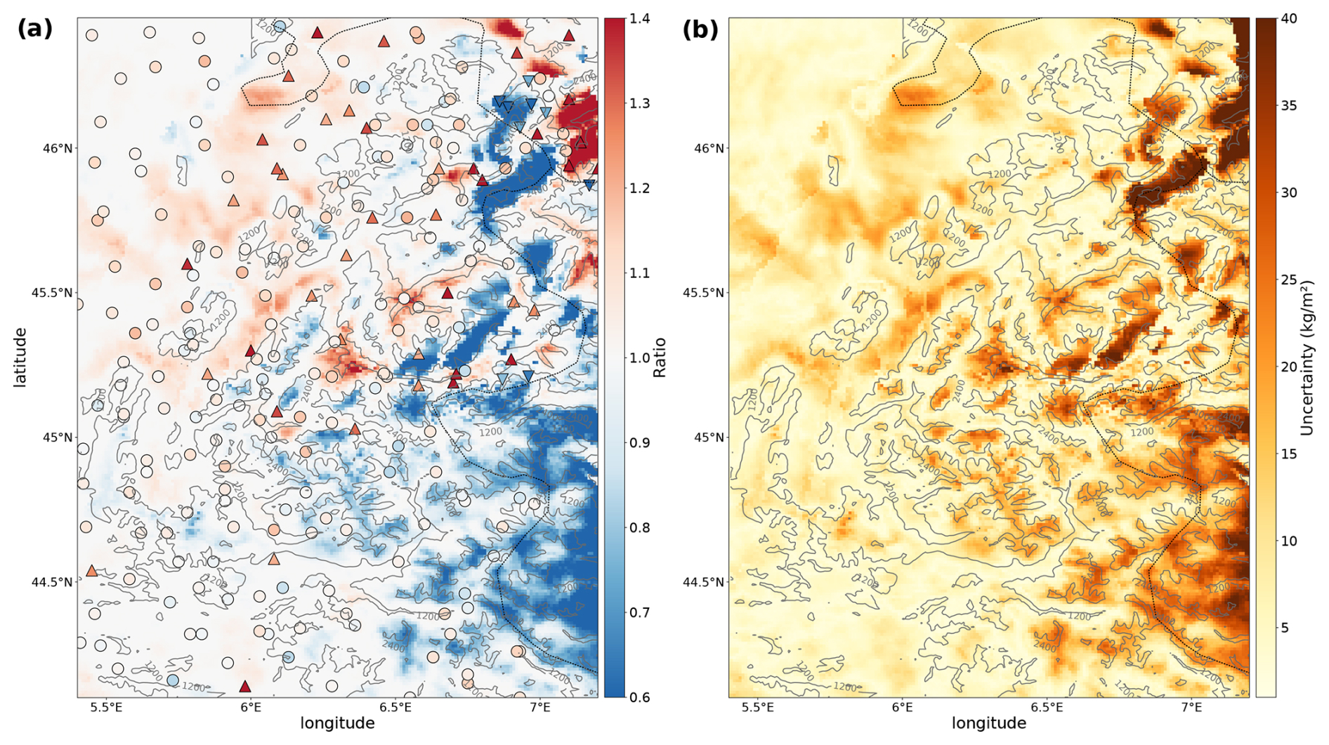
Figure 4 (a) Estimated climatological ratio ($\widehat{R}$) based on the mean ratios between ANTILOPE and automatic gauge precipitation measurements and (b) uncertainty index (U) obtained using the method described in Sect. 3.1.1. The grey lines indicate the 1200, 2400, and 3600 m isolevels to illustrate the relationship between the estimated ratio and the relief.

3.1.4 Dynamic correction of ANTILOPE daily precipitation fields

To deal with the unrealistic spatial patterns described in Sect. 3.1, a pre-processing step is applied to the daily ANTILOPE precipitation estimation fields and is illustrated in Fig. 5. A first correction is applied to mitigate climatological errors using the estimated climatological ratio field obtained in Sect. 3.1.1 (Figs. 4a and 5b). For each pixel i of the domain with a precipitation value $P_i^{\text{ANT}}$ estimated by ANTILOPE (Fig. 5a), the precipitation value after climatological correction (Fig. 5c) is given by $P_i^d=\frac{P_i^{\text{ANT}}}{R_i}$.

A modified weighted moving average (WMA) filter is then applied using the uncertainty index (Figs. 4b and 5c) obtained with the method described in Sect. 3.1.1. The WMA window includes all pixels within a d₀=20 km radius from pixel i (red circle in Fig. 5c). To estimate the filtered precipitation of pixel i, each pixel k within this window is assigned a weight $c_{ik}=\frac{\mathrm{1}-d_{ik}/d_{\mathrm{0}}}{U_k/U_{\mathrm{0}}}$, where d_ik is the distance to the pixel at the centre of the moving window, U_k is the uncertainty index of pixel k (see Sect. 3.1), and U₀=1 kg m⁻² is a normalisation factor. Considering all n pixels of the window, the weighted mean precipitation ($\stackrel{\mathrm{‾}}{P_i^d}$) and the variance (V_i) of all weighted precipitation values over the window associated to pixel _i are

$$\begin{array}{}\text{(10)}& -\left\{\begin{array}{c}\stackrel{\mathrm{‾}}{P_i^d}=\frac{\mathrm{1}}{C_i}{\sum }_{k=\mathrm{1}}^n{c}_{ik}{P}_{ik}^d\\ V_i=\frac{\mathrm{1}}{C_i}{\sum }_{k=\mathrm{1}}^n{c}_{ik}(P_{ik}^d-\stackrel{\mathrm{‾}}{P_i^d}{)}^{\mathrm{2}}\end{array}\mathrm{where}{C}_i=\sum _{k=\mathrm{1}}^n{c}_{ik}.\right.\end{array}$$

While a standard WMA filter would have regarded $\stackrel{\mathrm{‾}}{P_i^d}$ as the new precipitation estimate for pixel i, in this work the filtered value is combined with the local value with respective weights depending on the estimated spatial error (Fig. 5e):

$$\begin{array}{}\text{(11)}& P_i={\displaystyle \frac{P_i^d{c}_{ii}+\stackrel{\mathrm{‾}}{P_i^d}\frac{C_i}{n}}{c_{ii}+\frac{C_i}{n}}}.\end{array}$$

This weighted correction ensures that a pixel with a low estimated spatial error ($c_{ii}\mathit{>>}\frac{C_i}{n}$) is not affected by the WMA filter, while a pixel with a high estimated spatial error ($c_{ii}\ll \frac{C_i}{n}$) is closer to the average precipitation value in the localisation area.

The observation error (Fig. 5f) is finally defined as the weighted spatial standard deviation of the daily precipitation over this window:

$$\begin{array}{}\text{(12)}& E_i=\sqrt{V_i}.\end{array}$$

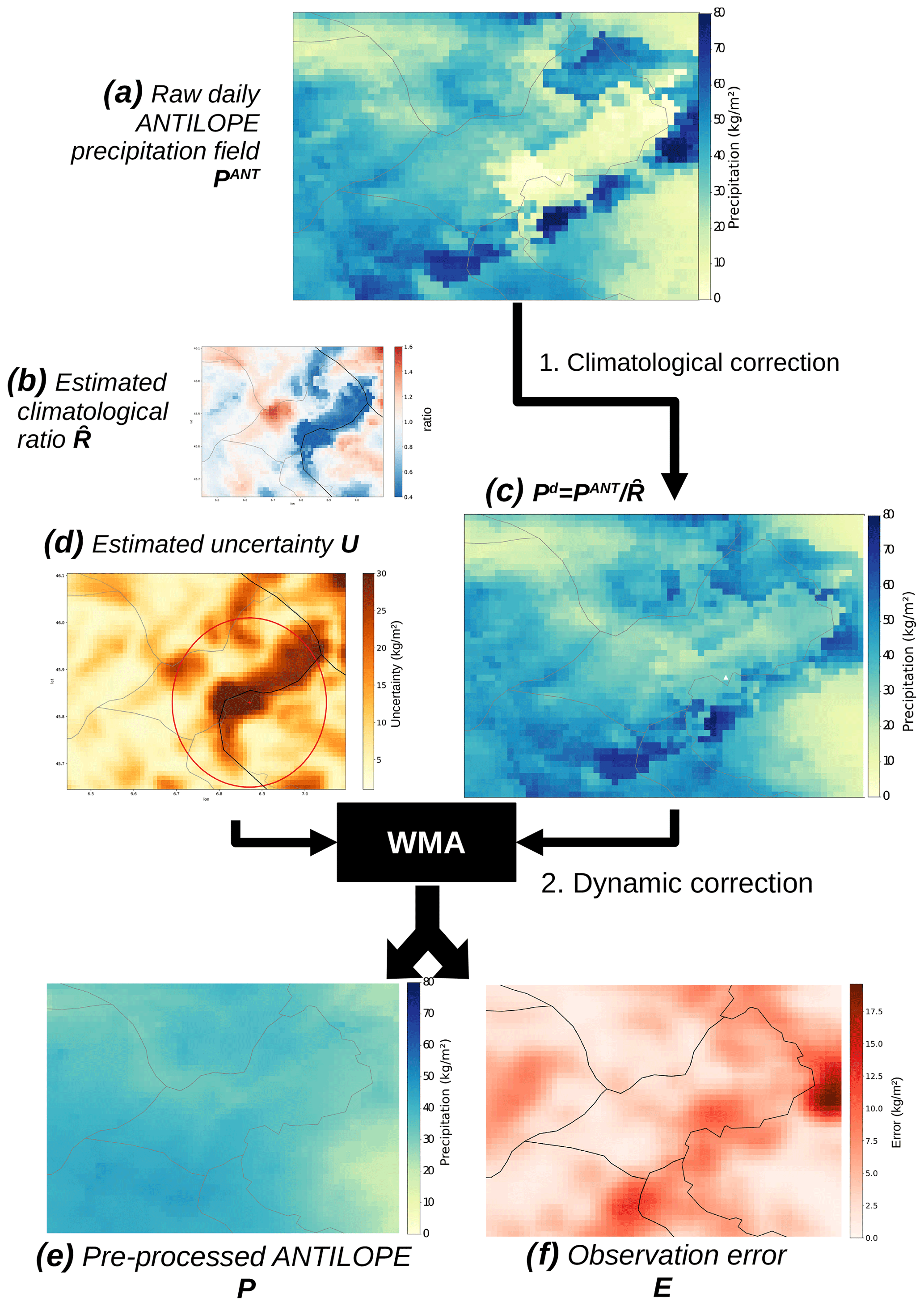
Figure 5 Illustration of the ANTILOPE pre-processing step applied for daily precipitation fields. First the climatological ratio ($\widehat{R}$) estimated with the method described in Sect. 3.1.1 is used as a climatological correction factor to mitigate systematic errors. The resulting precipitation field (P^d) is then filtered with a modified weighted moving average (WMA) method, which produces a smoother output daily precipitation field (P) and an associated error field (E). The weights used in the WMA step are a combination of an inverse distance weighting and the uncertainty index (U) estimated using the method described in Sect. 3.1.1.

3.2 Ensemble analysis

Three different methods are proposed to produce ensemble precipitation analyses of daily precipitation fields based on the pre-processed ANTILOPE precipitation fields obtained with the algorithm described in Sect. 3.1.4. Two of these methods are based on ensemble data assimilation algorithms that combine an observation (pre-processed ANTILOPE precipitation field) and an ensemble of NWP model outputs (post-processed PEAROME precipitation fields).

3.2.1 Random sampling

The first ensemble analysis method uses output fields of the ANTILOPE pre-processing step described in Sect. 3.1.4 to construct 16 precipitation fields by random perturbations around the corrected precipitation field $\stackrel{\mathrm{̃}}{P^i}$ (Fig. 5e).

We have chosen to separate the spatial and dynamical components of the observation error in a similar way to Villarini et al. (2014). The spatial observation error E_i accounts for the intrinsic spatial structure of the error associated with measurement issues in the ANTILOPE product described in Sect. 3.1 and comes from the pre-processing step (Sect. 3.1.4). The dynamic error is associated with the uncertainty of each individual event and is expressed as a fraction of the precipitation intensity. The magnitude of this error has been estimated from the linear regression between the ANTILOPE precipitation intensity and the associated error (not shown) and is set at 30 % of the precipitation intensity.

The random perturbation for a given ensemble member m is then determined by two different values:

• N^m is sampled from a normal distribution centred on 0 and with a variance of 1 and applied as a multiplicative factor to the spatial component of the error.

• G^m is sampled from a gamma distribution (with a shape parameter k=2 and a scale parameter $\mathit{\theta }=\sqrt{\mathrm{1}/k}$, ensuring a variance of 1) shifted by kθ so that the mean of the distribution is 0.

For each pixel i of the domain with a corrected precipitation P_i (Eq. 11) and an associated error E_i (Eq. 12), the precipitation in member m of the output ensemble is thus

$$\begin{array}{}\text{(13)}& P_i^m=max\left(P_i\right(\mathrm{1}+\mathrm{0.3}{G}^m)+N^m.E_i,\mathrm{0}).\end{array}$$

Drawing random values from distributions with a mean centred on 0 ensures that the resulting ensemble mean is expected to be P_i, unless the magnitude of the spatial error is greater than the precipitation value itself (in which case the 0 kg m⁻² lower bound may shift the ensemble mean upwards).

This random sampling (RS) analysis is the direct translation of the ANTILOPE pre-processing step, which produces a corrected precipitation field and associated error, into an ensemble analysis. It can be considered a benchmark product for ensemble analysis.

3.2.2 Particle filter

The second ensemble analysis is based on particle filter theory. Particle filters (PFs) are sequential Monte Carlo algorithms commonly used for data assimilation in non-linear systems (van Leeuwen, 2009). These methods are based on the approximation of the model probability density function (PDF) by an ensemble of model states (called ensemble members and denoted X in the following equations). When an observation P_i is available, this ensemble of model states is updated in two steps. First, the different members are weighted according to their likelihood (distance to the observation). Then, the model state PDF is updated by resampling the different members according to their weights: members with high weights are replicated, while those with lower weights are dropped. To deal with the known problems of the PF algorithm for large numbers of observations, Snyder et al. (2008) suggest reducing the dimension of the problem by splitting a large set of observations into smaller subsets. Here we chose to apply the particle filter algorithm for each pixel independently, reducing the problem dimension to one observation for a 16-member ensemble. Thus, the likelihood of the PEAROME precipitation forecast $X_i^m$ of member m over a pixel i can be simply formulated as a function of the corresponding ANTILOPE pre-processed precipitation P_i (Eq. 11) and its associated error E_i:

$$\begin{array}{}\text{(14)}& L_i=e^{-{\left(\frac{(X_i^m-P_i)}{E_i}\right)}^{\mathrm{2}}}.\end{array}$$

The main disadvantage of this local approach is the loss of spatial consistency. In fact, the analysed precipitation accumulation of neighbouring pixels can be obtained from combinations of different members. To obtain consistent precipitation fields, a field reconstruction step based on an ensemble copula coupling method (Schefzik et al., 2013) is applied during the resampling step. This resampling procedure is based on preserving the rank structure of the ensemble members from the original ensemble to the analysed one, ensuring, for example, that the same member has the highest precipitation value on a pixel before and after the analysis. In this way, large-scale structures are preserved in the analysis, although local discrepancies may persist.

3.2.3 Ensemble Kalman filter

The last ensemble analysis is based on the ensemble Kalman filter (EnKF) algorithm (Evensen, 2003). EnKFs are Monte Carlo implementations of the Kalman filter (Kalman, 1960), where an ensemble of simulations is used to sample the model state (background) distribution. The main advantage over the PF is that it preserves the spatial consistency of the analysed fields. We have chosen an approach inspired by that of Atencia et al. (2020b), using only the analysis step of the EnKF, which consists of updating each ensemble member with the information coming from an observation. It is assumed that the cross-correlations between the background and the observation are negligible so that each pixel of the domain is processed independently. For a given pixel i, the precipitation estimated by the ensemble member m ($X_i^m$) is pulled towards the corresponding observation (ANTILOPE pre-processed precipitation P_i from Eq. 11):

$$\begin{array}{}\text{(15)}& \stackrel{\mathrm{̃}}{X_i^m}=X_i^m+K_i(P_i-X_i^m),\end{array}$$

where the so-called gain factor K_i defines the relative influence of the original background value and the observation, based on the observation error E_i defined in Eq. (12) and the background error represented by the 16-member (N=16) ensemble spread $B_i=\frac{\mathrm{1}}{N-\mathrm{1}}{\sum }_{m=\mathrm{1}}^N(X_i^m-\stackrel{\mathrm{‾}}{X_i^m})(X_i^m-\stackrel{\mathrm{‾}}{X_i^m})$:

$$\begin{array}{}\text{(16)}& K_i=B_i(B_i+E_i{)}^{-\mathrm{1}}.\end{array}$$

3.3 Evaluation method

The aim of this work is to produce an ensemble precipitation analysis with a resolution of 1 km over the French Alps, which should ideally fulfil the standard requirements expected from ensemble modelling systems (reliability and resolution). This ensemble analysis should reduce the systematic biases of the ensemble mean and improve precipitation estimation as compared to other existing products. Finally, spatial artefacts affecting the radar-based precipitation fields must not be propagated to the analysis, meaning that each individual ensemble member should feature realistic spatial structures.

While the first three requirements can be evaluated at the point scale with the available independent observations of the ski-resort network, the lack of a spatialised reference observation of the precipitation fields implies that an objective evaluation of the spatial structure of the analysed fields is not directly possible at this stage.

The different products were evaluated during the 2021/2022 winter season. Each available ski-resort observation of 24 h precipitation at 08:00 CET was compared with the corresponding 24 h precipitation estimate at 07:00 UTC on the corresponding 1 km pixel for each product. First, a comprehensive evaluation of existing precipitation estimation products is provided. In the case of deterministic products, this evaluation focuses on the magnitude of systematic biases and their spatial distribution, as well as on the consistency of the spatial structure of the precipitation fields. For ensemble products, ensemble characteristics such as the spread skill are also taken into account. As all proposed ensemble analysis methods rely on a pre-processing of the ANTILOPE precipitation estimation product, an objective evaluation of the pre-processing step and its performance compared to existing products is provided. A subjective comparison of the spatial structures of the precipitation fields is also discussed. Finally, the three ensemble analysis methods are evaluated, and their performances are compared in terms of mean bias, spread skill, and overall predictive value added.

Biases, ratios, and root mean square deviations are computed for each reference station by comparing the estimated and observed time series of 24 h precipitation records. For ensemble products, the estimated value is taken as the ensemble mean. The predictive added value of the different products is assessed using two probabilistic scores commonly used for ensemble prediction systems: the Brier score (BS; Brier, 1950) and the continuous ranked probability score (CRPS; Matheson and Winkler, 1976; Candille and Talagrand, 2005). More details on these scores can be found in Appendix B. Another important aspect of ensemble forecasting is the reliability of the ensemble spread: an ensemble forecasting system is reliable if the magnitude of its spread for different events and locations matches the associated spread of the ensemble mean error. This can be inferred from a scatter plot of the ensemble spread against the ensemble mean error (Hopson, 2014).

4 Results

4.1 Evaluation of existing precipitation products

The main results of the evaluation of the existing products (PANTHERE, gauge kriging, ANTILOPE, and post-processed PEAROME) are summarised in Fig. 6, showing the distributions of the root mean square deviation from the ski-resort reference observations for all data (Fig. 6a) and for observed precipitation events above 10 kg m⁻² in 24 h only (Fig. 6b). This figure shows that the precipitation estimation from the network of automatic observation stations (KRIGING) performs better than the estimation from radar measurements only (PANTHERE) in mountainous areas. The RMSE of the combination of these two sources of information (ANTILOPE) is of the same order of magnitude as that of the KRIGING product but is sometimes improved for precipitation events above 10 kg m⁻²in24 h (b). Similar results are obtained when only snowfall events are considered (Fig. C2). Other results (frequency of relative errors less than 20 %, not shown) also support the choice of ANTILOPE as the best precipitation product available for an ensemble analysis system, especially since ANTILOPE performs equally well when only solid precipitation is considered (see Fig. C2 in Appendix C). Figure 7a shows that the mean ratio between ANTILOPE-estimated precipitation and the corresponding ski-resort reference observations can reach both very high (above 1.5, in red) and very low (below 0.5, in black) values, even for stations separated by only a few kilometres. However, the spatial distribution of ANTILOPE's performance shows that even if there is no widespread systematic bias, there is a high spatial variability in its performance. Moreover, the lack of evaluation stations at high altitudes or near mountain ridges does not allow for good documentation of the spatial artefacts already discussed in Sect. 3.1.

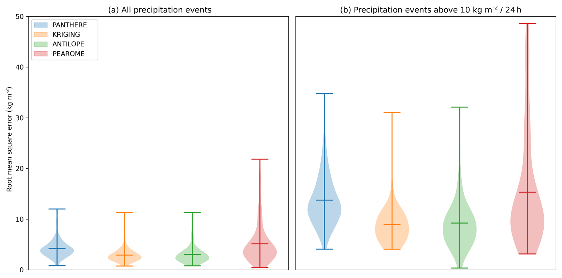
Figure 6 Distribution of the root mean square deviation of the existing precipitation estimation products from all ski-resort reference observations of daily precipitation (a) and daily precipitation above 10 kg m⁻² (b) over all evaluation stations. Precipitation estimates come from radar-only observations (PANTHERE), a kriging of gauge observations (KRIGING), a fusion of radar and gauge observations (ANTILOPE), and the ensemble mean of the post-processed high-resolution ensemble NWP model (PEAROME).

Finally, the RMSE of the PEAROME ensemble mean is much higher than that of all observation-based products (see Fig. 6). This indicates that even after statistical post-processing, PEAROME forecasts provide a less reliable estimate of precipitation than observation-based products. An evaluation using metrics specifically adapted to ensemble forecasting, such as the Brier score (BS) or the continuous ranked probability score (CRPS), shows that the probabilistic nature of PEAROME does not compensate for deficiencies in deterministic estimation (Fig. 9).

4.2 Evaluation of precipitation analyses

4.2.1 Impact of the pre-processing procedure

The ensemble precipitation analyses in this study are based on the ANTILOPE pre-processing step described in Sect. 3.1.4, which relies on the error estimation method described in Sect. 3.1.1. Figure 7b demonstrates the ability of this method to identify ANTILOPE biases, showing the same information as Fig. 7a but with unbiased precipitation estimates using the ratio from Fig. 4a. Spatial artefacts that are visible in the yearly precipitation accumulation of Fig. 7a appear to be reduced in Fig. 7b. In addition, the mean ratio with reference ski-resort observations after climatological correction is often closer to 1 (green dots) than that for raw ANTILOPE precipitation estimates.

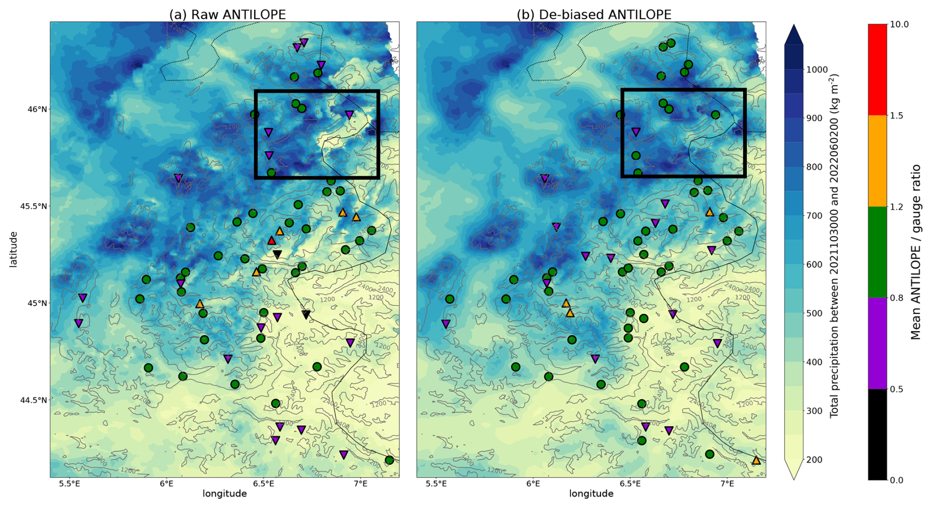
Figure 7 Yearly ANTILOPE precipitation accumulation over the entire French Alps domain and mean ratio with the available evaluation data from the ski-resort network before (a) and after (b) application of the climatological correction factor obtained by the observation error estimation method. The marker associated with each evaluation station is a circle if the ratio between ANTILOPE and the reference gauge precipitation estimates is not considered significant (between 0.8 and 1.2) and a triangle facing up (resp. down) if this ratio is significantly higher (resp. lower) than 1. The black rectangle indicates the Mont Blanc area from which the precipitation fields shown in Figs. 3 and 5 are derived.

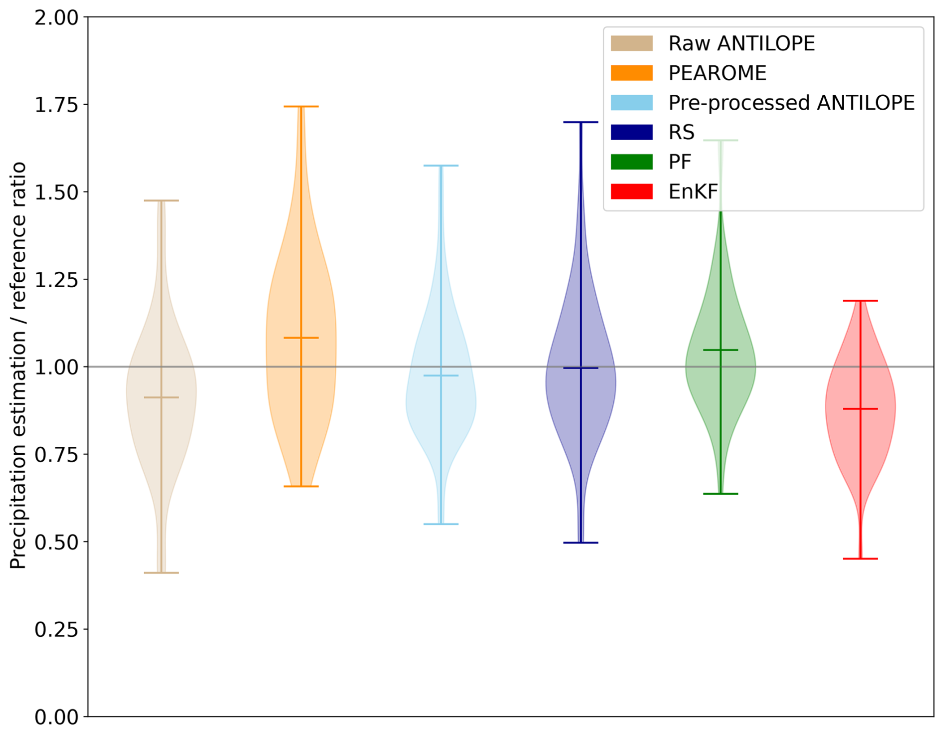
Figure 8 Ratio between estimated and observed accumulated precipitation over all ski-resort reference stations for the different methods assessed in this study.

Figures 8 and 9 show the performance of the full pre-processing step. The error estimation method reduces biases with ratios closer to 1 after the ANTILOPE pre-processing step (light blue) compared to before (brown), as confirmed by Fig. 8. In addition, Fig. 9 shows that this pre-processing step improves both CRPS and BS, regardless of the precipitation threshold.

4.2.2 Skill of ensemble analyses

All ensemble analyses (RS, PF, and EnKF) evaluated in Figs. 8 and 9 show better performance than the pre-processed ANTILOPE and PEAROME products respectively. Figure 9a shows a clear improvement of the BS for the three ensemble analysis methods, which all have similar performance for low- to moderate-precipitation events (up to 10 kg m⁻² in 24 h). However, for precipitation above 10 kg m⁻², the basic RS method outperforms the two methods based on ensemble data analysis. For precipitation events above 25 kg m⁻², the PF and EnKF analyses do not perform significantly better than the deterministic ANTILOPE pre-processing. This result is confirmed by the CRPS values (Fig. 9b), which are significantly lower for the RS analysis than for the PF and EnKF analyses.

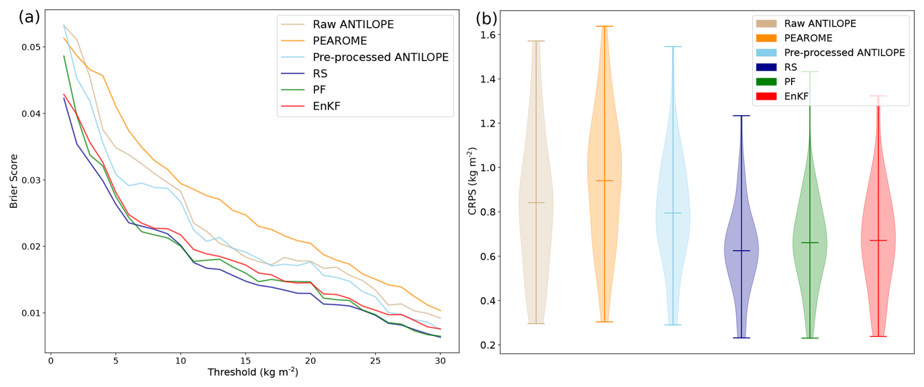
Figure 9 Evolution of the mean Brier score over all evaluation stations and dates for different daily precipitation thresholds ranging from 1 to 30 kg m⁻² (a). Distribution of the mean continuous ranked probability score over the reference stations (b). Six precipitation estimation products are shown: existing products in orange shades, deterministic products in light colours, and ensemble products in dark colours.

4.2.3 Spread-skill consistency

The spread of the raw PEAROME ensemble and the three ensemble analyses is shown in Fig. 10 as a function of the ensemble mean. Ideally, the spread should be of the same magnitude as the quadratic error of the ensemble mean (along the one-to-one line) as described by Hopson (2014). The post-processing of the PEAROME ensemble (Fig. 10a) is specifically designed to optimise statistical ensemble properties such as the mean spread. The magnitude of the ensemble spread is consistently comparable to the magnitude of the ensemble mean error, with approximately the same mean value (indicated by the dashed red lines).

The spread skill of the RS analysis (Fig. 10b) shows that the magnitude of the ensemble spread matches the magnitude of the ensemble mean error, with the spread on average being slightly higher than the error (dashed red lines). The blue regression line shows that high errors also tend to be underestimated by the ensemble spread but not as much as for the raw PEAROME product. The RS ensemble spread is more often close to 0 kg m⁻², indicating a higher confidence in the precipitation estimate than in the PEAROME ensemble.

Figure 10c and d show that the spread of the two ensemble analyses based on ensemble data assimilation methods clearly underestimates the magnitude of the ensemble mean error. The spread of both analyses barely exceeds 10 kg m⁻², while the ensemble mean error is often above 15 kg m⁻².

It is also worth noting that the ensemble mean error of the three ensemble analyses is on average significantly lower than that of the PEAROME ensemble (vertical dashed red lines indicate an error almost twice lower) and does not reach the same extreme values (in particular, the RS analysis mean error exceeds 25 kg m⁻² only once).

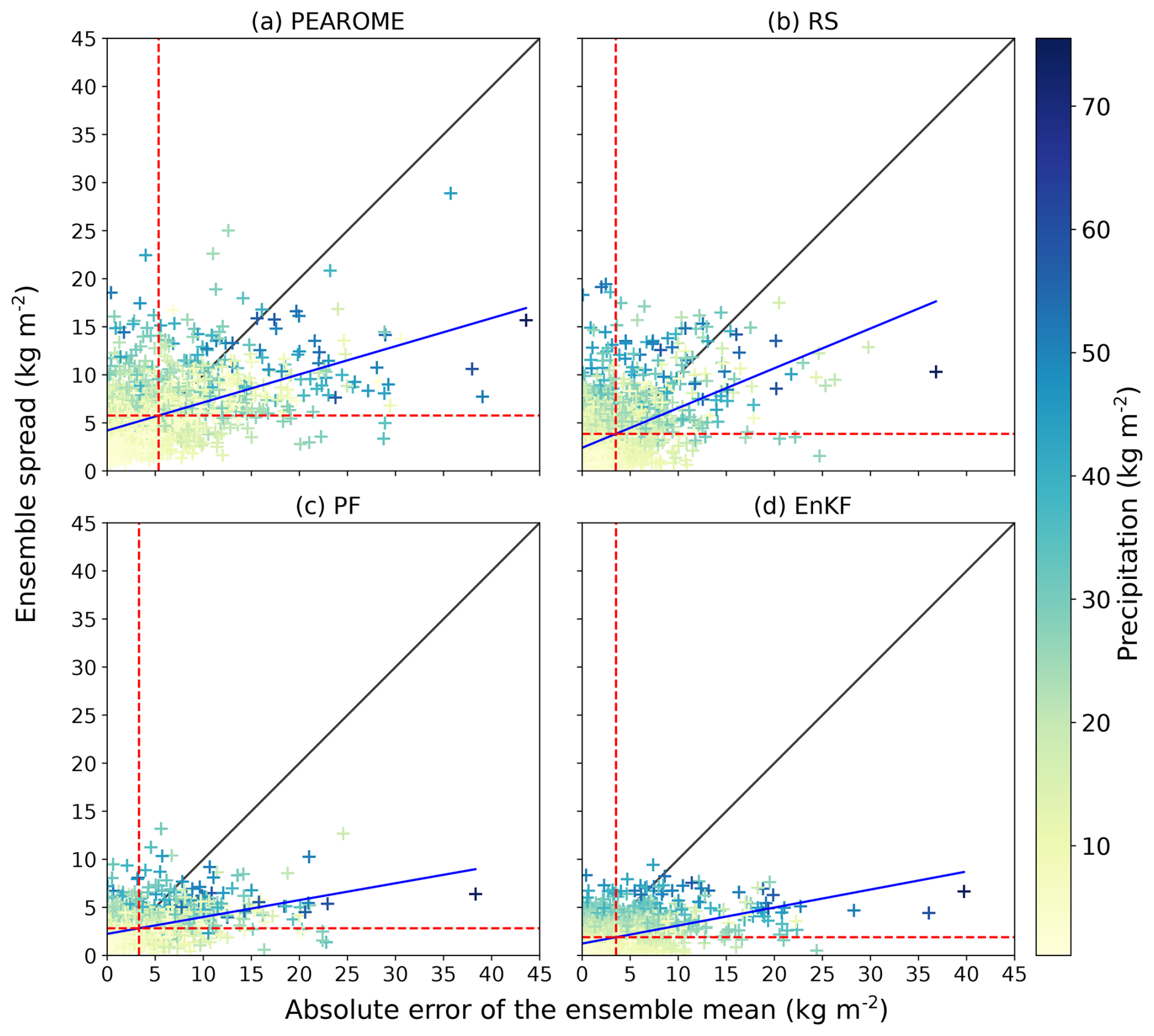
Figure 10 Spread skill of the different ensemble products. Each cross represents a specific evaluation point and date, and its colour indicates the corresponding 24 h precipitation. The blue line is the regression line of the scatter plot. The horizontal (resp. vertical) red line shows the mean ensemble error (resp. ensemble spread).

4.2.4 Spatial patterns

Figure 11 shows an example of four precipitation fields for each of the four ensemble products over the Mont Blanc area (see Fig. 1) for the same date as the fields in Fig. 5. This illustrates the spatial variability of precipitation produced by the different analysis methods. The RS analysis produces very smooth fields, similar to the corresponding pre-processed ANTILOPE field (Fig. 5e), but with different precipitation intensities. The fields resulting from the PF and EnKF analyses are a combination of this pre-processed ANTILOPE field and the corresponding PEAROME fields, also visible in Fig. 11e and f. Despite the field reconstruction step described in Sect. 3.2.2, the application of the particle filter algorithm at the pixel scale results in rather noisy fields. EnKF precipitation fields better preserve the spatial variability of the corresponding PEAROME fields, with a convergence of intensity towards the pre-processed ANTILOPE field. As explained in Sect. 3.3, the lack of spatialised reference observations prevents any objective evaluation of the spatial structures of the different analyses, except that noisy PF precipitation fields are a serious shortcoming for further exploitation of this precipitation analysis.

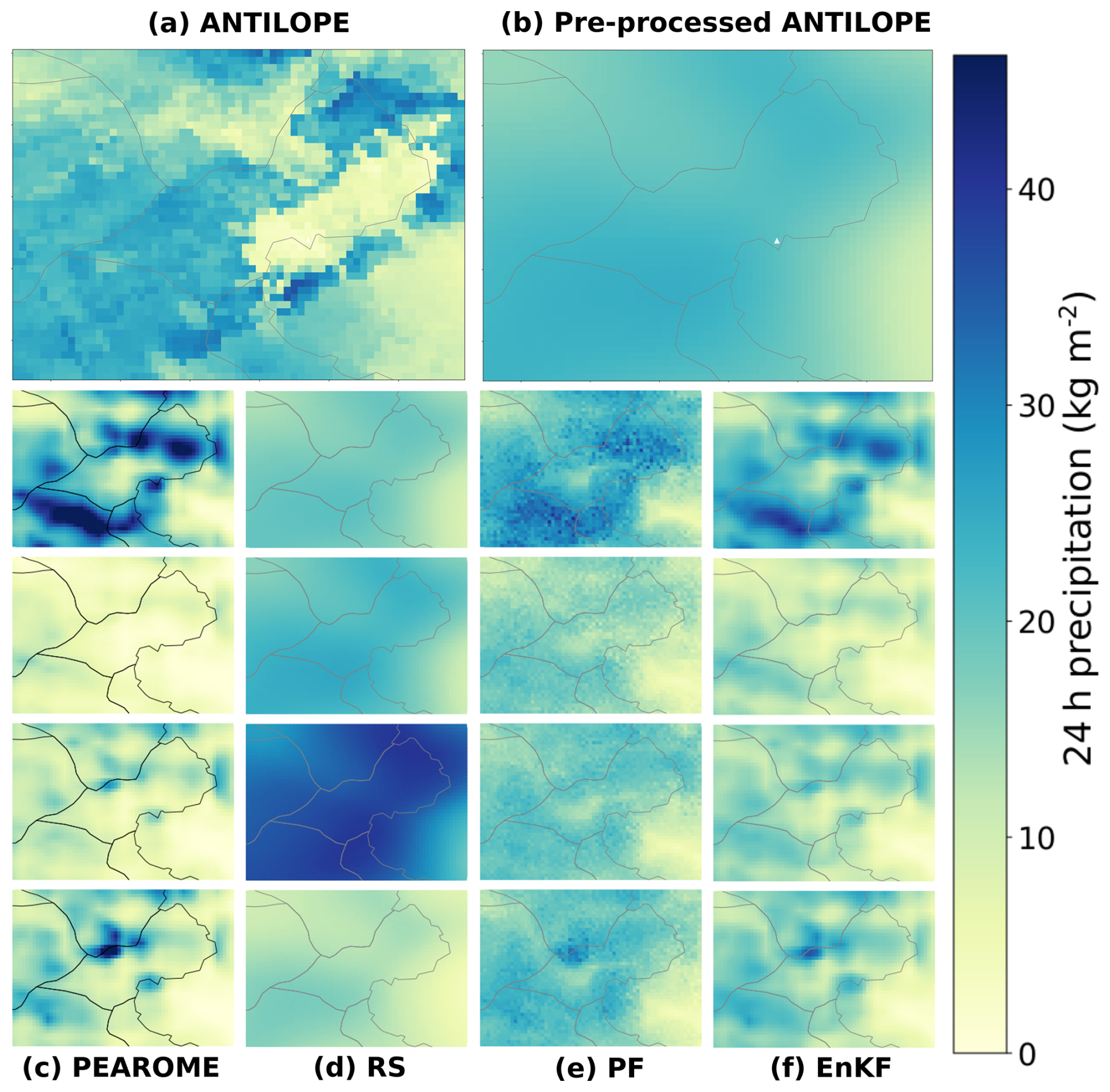
Figure 11 Example of 24 h precipitation fields of 4 December 2021 over the Mont Blanc area (see Fig. 1). (a) Raw ANTILOPE observation. (b) Pre-processed ANTILOPE field. (c) Members 1 to 4 of the post-processed PEAROME ensemble. (d) Members 1 to 4 of the random sampling analysis around the pre-processed ANTILOPE field (b). (e) Members 1 to 4 of the particle filter analysis. (f) Members 1 to 4 of the ensemble Kalman filter analysis. The full 16-member ensembles for each ensemble product are shown in Appendix C.

5 Discussion

5.1 Precipitation estimation products in mountainous areas

The evaluation of different precipitation products with an independent observation network in ski resorts (Sect. 4.1) shows that observation-based estimates provide better results than forecasts from the PEAROME ensemble, even after a post-processing step designed to remove biases and improve reliability. This contradicts, at least for the French Alps, the conclusion of Lundquist et al. (2019) that high-resolution precipitation models outperform observations in mountainous areas. However, these products have complementary qualities and shortcomings.

Although radar observation provides spatialised information, its quality is very heterogeneous in space and suffers from important limitations in mountainous areas. Ground clutter and partial beam blocking are common due to the complex topography, and the management of these disturbances in the radar processing algorithm described in Sect. 2.1 does not compensate for the loss of information.

The most obvious effect of the interception of a radar beam by a mountain is a significant underestimation of the mean precipitation above the pixels affected by ground clutter, which produces spatial artefacts in the precipitation fields. This degradation of precipitation estimation due to increased height of the lowest usable radar measurement above ground is particularly pronounced for stratiform precipitation systems with relatively small vertical extent (Germann et al., 2022). This is the case for the majority of the winter precipitation events in the French Alps on which this study focuses, thus limiting the extrapolation of its conclusions to convective situations.

Radar-based precipitation estimates are also less reliable over valleys, where the height difference between the radar beams and the ground is more important (Fig. 2), and precipitation variations below the beams are neglected. However, this problem is compensated for in the ANTILOPE product by the use of many in situ measurements at these altitudes (Fig. 1). On the contrary, higher-elevation areas are under-sampled (Fig. 1 shows that only 31 out of 512 available automatic gauges are above 2000 m a.s.l.), so radar measurement problems at these altitudes cannot be properly corrected. The lack of reference observations over ridges (Fig. 1) also makes it impossible to assess the magnitude of the error at these altitudes. This led us to develop a pre-processing step, described in Sect. 3.1.4, to mitigate the resulting spatial artefacts and provide a spatialised assessment of the highly variable uncertainty in this product.

5.2 Observation error

Most of the results of this study are based on the spatialisation of the error associated with the ANTILOPE precipitation product. Despite the positive results at the local scale shown in Sect. 4.2, this method has some limitations and possible improvements have been identified:

• The WMA filter described in Sect. 3.1.4 tends to smooth precipitation fields. This is a necessary compromise to remove unrealistic spatial patterns that would be very detrimental to snow modelling (with unrealistic snow amounts near ridges, as illustrated by Haddjeri et al., 2023, with the ANTILOPE raw product). However, it can potentially erase realistic spatial structures well detected by the radar, even if the formulation of Eq. (11) and the parameters in the error estimation method have been chosen to ensure minimal modification over pixels with no clear systematic errors. High-intensity precipitation kernels are therefore often smoothed by the pre-processing step, which may affect the detection of extreme events. The spatial structures of the analysed precipitation fields could not be evaluated with the reference dataset used in this study. An indirect evaluation of simulated snow depths based on the precipitation analyses presented here is planned in a future study, following the workflow already proposed by Haddjeri et al. (2023). In such a study, we will compare simulated snow depths with snow depth maps derived from high-resolution Pleiades satellite images (Deschamps-Berger et al., 2020) over the Grandes Rousses domain.

• The climatological approach of this method makes it highly dependent on ANTILOPE evolutions (changes in the algorithm, in the available radar, or in the in situ measurements used) so that regular recalibration would probably be required.

• Additional available radar information, not considered in this work, could also provide relevant information for the estimation of the observation error (height above ground of the lowest available radar beam, position of ground clutter, etc.).

• As most gauges are located in valleys or at low altitudes, the uncertainty index is generally higher at high altitudes (Fig. 4b). To mitigate the over-representation of low-elevation pixels in the WMA filter, the weights computed in the pre-processing step (Sect. 3.1.4) could take into account the elevation difference between pixels.

• The uncertainty information generated by the kriging with the external drift algorithm producing the raw ANTILOPE product could be used to improve the estimation of the associated observation error.

• The error estimation method described in Sect. 3.1.1 could be applied to daily precipitation fields in order to improve the handling of instances where the ANTILOPE error is significantly different from its climatological value.

5.3 Choice of the data assimilation method

The random sampling (RS) ensemble analysis combined with the pre-processing method described in Sect. 3.1.4 proved to fulfil most of the requirements for a suitable ensemble precipitation analysis in complex terrain, even if the accuracy of the spatial structures of the individual fields remains to be evaluated. This result is particularly promising for the future goal of assimilating satellite snow observations into snowpack simulations. It accurately accounts for precipitation uncertainties and thus addresses the main limitation raised by Cluzet et al. (2022) and Deschamps-Berger et al. (2022) to take full advantage of the assimilation of snow observations. It is based on a very simple ensemble generator and could probably be significantly improved using methods inspired by those reviewed in Mandapaka and Germann (2010). The RS analysis is also the most computationally efficient and requires less data handling.

On the contrary, the information provided by high-resolution NWP models may suffer from larger errors on average but is more physically consistent and can therefore be expected to have more spatially homogeneous errors than precipitation estimation derived from radar measurements. Ensemble forecasts also provide uncertainty information that is lacking in deterministic observational products. This motivated the use of the AROME climatology for the ANTILOPE pre-processing step and the PEAROME daily precipitation fields through data assimilation methods. However, the evaluation presented in Sect. 4.2 shows that most of the NWP added value comes from the use of the AROME climatology, at least at the local scale. In particular, the EnKF and PF analyses proved to be very under-dispersive. This deficiency could be very detrimental in snow simulation systems based on ensemble assimilation of snow observations with e.g. the particle filter (Cluzet et al., 2022; Deschamps-Berger et al., 2022), as in many cases no optimal scenario would be available among the backgrounds. The assimilation of snow observations would then fail to provide better estimates of snow conditions. The under-dispersion of both PF and EnKF analyses is an inherent aspect of these ensemble data assimilation algorithms: the main concept of these algorithms is to modify an ensemble of initial simulations (the background state) with the knowledge of an observation and its associated error. Both PF and EnKF methods ensure that the resulting analysed ensemble has a smaller dispersion than the background ensemble: the PF analysis is a sub-ensemble of the background ensemble, and the EnKF equations described in Sect. 3.2.3 imply a convergence of all background members to the observation as long as the observation error is comparable to the background one (Hotta and Ota, 2021). Thus, a well-dispersed background ensemble, such as the post-processed PEAROME ensemble used in this study, can only lead to under-dispersed analysed ensembles when PF or EnKF ensemble data assimilation algorithms are applied using observations with lower errors than the background. This is typically the case with the ANTILOPE product, at least where reference data are available. However, in instances where the ANTILOPE uncertainty is significantly higher than the PEAROME error, the impact of these algorithms on the background ensemble is minimal.

The consistency of the spatial structures produced by these analyses could not be objectively assessed. However, the PF analysis fields suffer from obvious spatial artefacts (even after a field reconstruction step). This PF method is also numerically more expensive when applied at the pixel scale, which can be a severe limitation for application over large areas. Applying the PF algorithm simultaneously to the whole domain would lead to degeneracy due to the very high number of available observations compared to the ensemble size. A compromise solution would be to apply the PF algorithm over well-chosen subdomains, as suggested by Cluzet et al. (2021), but this would require further strong hypotheses for the definition of the subdomains. Considering all these elements, the analysis method based on the EnKF algorithm is clearly more suitable than the one based on the PF, but it does not outperform the RS analysis based on observations only and relying on a simplistic ensemble generation method, at least at the local scale used for the evaluation in this study. This result implies that the information provided by direct radar and in situ precipitation measurements cannot be significantly improved by daily high-resolution NWP forecasts up to a 33 h lead time. However, only a spatialised evaluation could determine whether the spatial structures produced by a high-resolution NWP model and transferred to the EnKF analysis (see Fig. 11) can prove to be complementary information with added value.

6 Conclusions

This study first provides an evaluation of state-of-the-art precipitation estimation products available over the French Alps. It focuses in particular on radar-based observational products, the quality of which is not well documented but is often considered to be poor in complex terrain. Our evaluation against an independent dataset of 24 h precipitation accumulation from ski resorts showed that radar measurements combined with precipitation estimation from an automatic gauge network provide the best precipitation estimates among all products considered. In particular, the performance of such a product was shown to be significantly better than the output of the most advanced high-resolution numerical weather prediction model available in this study's area. This is noteworthy because previous studies have suggested that these models have outperformed observation-based precipitation estimates in some areas (Lundquist et al., 2019). However, significant shortcomings related to expected radar measurement problems were also identified. In this study, we developed a method to estimate the spatial distribution of climatological errors associated with unrealistic spatial patterns, such as unrealistically low accumulation over ridges, in annual and daily precipitation fields. This method has been developed and evaluated for the French Alps but can be applied to any mountainous area covered by similar precipitation estimation products. A correction algorithm was applied to daily precipitation estimates using the mean precipitation gradient from the AROME NWP model. Although no objective evaluation of the spatial structure of the daily precipitation fields produced by this method could be carried out, this correction seems to be able to mitigate spatial artefacts visible in the annual precipitation accumulations and proved to improve precipitation estimates over a set of reference stations. Some possible refinements of the method have also been outlined for future improvements, such as taking advantage of additional available radar information or the inclusion of topographic criteria in the weighting step.

Three different ensemble analysis methods were then implemented based on the corrected precipitation fields obtained by the previous method. A first reference analysis randomly samples values around these observed precipitation fields from their estimated error. Analyses were then conducted using two ensemble data assimilation algorithms, namely the particle filter and the ensemble Kalman filter. These algorithms were used to combine the corrected precipitation fields with those produced by a high-resolution numerical weather prediction model ensemble. The aim was to explore the complementarity of these two sources of information. The method based on the particle filter turned out to be both more numerically expensive and to suffer from major drawbacks, especially regarding the excessive noise in the produced precipitation fields. The method based on the ensemble Kalman filter proved to be more suitable but did not outperform the ensemble analysis based only on the reference observation dataset used in this study. However, the spatial structures obtained by both methods are significantly different, and a spatialised evaluation will be necessary to determine which is the most appropriate.

Therefore, the next step will be to use the ensemble precipitation analyses described in this article to force a snow model. This will allow the resulting simulated snow properties to be compared with corresponding satellite observations thanks to the memory effect of the snowpack, which ensures a strong relationship between the state of the snowpack and past snowfall (Haddjeri et al., 2023). The main challenge of this indirect evaluation of precipitation analyses will be the introduction of additional uncertainties such as the height of the rain–snow limit (Vionnet et al., 2022) and the errors in the snowpack model (Essery et al., 2013; Lafaysse et al., 2017).

Appendix A: ANTILOPE climatological error estimation method illustration

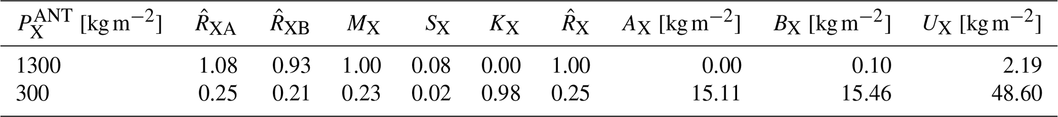
This section is a numerical illustration of the estimation of the ANTILOPE climatological error on a specific pixel, designated X, based on two nearby available gauges on pixels A and B, which are situated at the same distance from pixel X (d_AX=d_BX and w_AX=w_BX as illustrated in Fig. A1). It is assumed that the ANTILOPE product provides an unbiased estimation of precipitation accumulation for pixels A and B. This implies that the ANTILOPE yearly precipitation accumulation is the same as the one measured at the gauge: $P_{\mathrm{A}}^{\mathrm{ANT}}=P_{\mathrm{A}}^{\mathrm{GAUGE}}=\mathrm{300}$ kg m⁻² and $P_{\mathrm{B}}^{\mathrm{ANT}}=P_{\mathrm{B}}^{\mathrm{GAUGE}}=\mathrm{700}$ kg m⁻² (thus, $R_{\mathrm{A}}^{\mathrm{GAUGE}}=R_{\mathrm{B}}^{\mathrm{GAUGE}}=\mathrm{1}$). Furthermore, it is assumed that the AROME climatology exhibits 4 times more precipitation on pixel X ($P_{\mathrm{X}}^{\mathrm{ARO}}=\mathrm{2000}$ kg m⁻²) than on pixel A ($P_{\mathrm{A}}^{\mathrm{ARO}}=\mathrm{500}$ kg m⁻²) and twice the precipitation than on pixel B ($P_{\mathrm{B}}^{\mathrm{ARO}}=\mathrm{1000}$ kg m⁻²).

Numerical results of the error estimation method are given for two different values of ANTILOPE precipitation accumulation on pixel X ($P_{\mathrm{X}}^{\mathrm{ANT}}$) and are summarised in Table A1. The first case ($P_{\mathrm{X}}^{\mathrm{ANT}}=\mathrm{1300}$ kg m⁻²) illustrates a situation where ANTILOPE is free of artefacts on pixel X. This means that the ANTILOPE yearly precipitation accumulation is consistent with the values on pixels A and B, as well as with the AROME precipitation ratios. In this situation, estimated ratios from reference pixels A and B (${\widehat{R}}_{\mathrm{XA}}$ and ${\widehat{R}}_{\mathrm{XB}}$) are both relatively close to 1 (1.08 and 0.93 respectively). Therefore, the estimated ratio on pixel X (${\widehat{R}}_{\mathrm{X}}$) is very close to 1, and the associated uncertainty (U_X=2.2 kg m⁻²) is close to the minimum value possible (2 kg m⁻²; see Sect. 3.1.3). The second case illustrates a situation where ANTILOPE is affected by ground clutter on pixel X. This has been identified as leading to unrealistically low precipitation accumulations (in this example, $P_{\mathrm{X}}^{\mathrm{ANT}}=\mathrm{300}$ kg m⁻²). In this case, ratios estimated from the reference pixels A and B are both significantly lower than 1 and consistent with each other, leading to an estimated ratio ${\widehat{R}}_{\mathrm{X}}=\mathrm{0.23}$ kg m⁻². The associated uncertainty is consequently very high (U_X=48.6 kg m⁻²). The contribution of the first term of Eq. (8) is $(\mathrm{1}+K_{\mathrm{X}})\times (A_{\mathrm{X}}+\mathrm{1})=\mathrm{31.8}$, twice the contribution of the second term $(\mathrm{1}+K_{\mathrm{X}})\times (A_{\mathrm{X}}+\mathrm{1})=\mathrm{16.8}$. The contribution of the first term for approximately two-thirds of the ultimate uncertainty can be interpreted as a predominance of an identified systematic bias in the uncertainty estimation over diverging information brought about by the presence of gauges in pixels A and B.

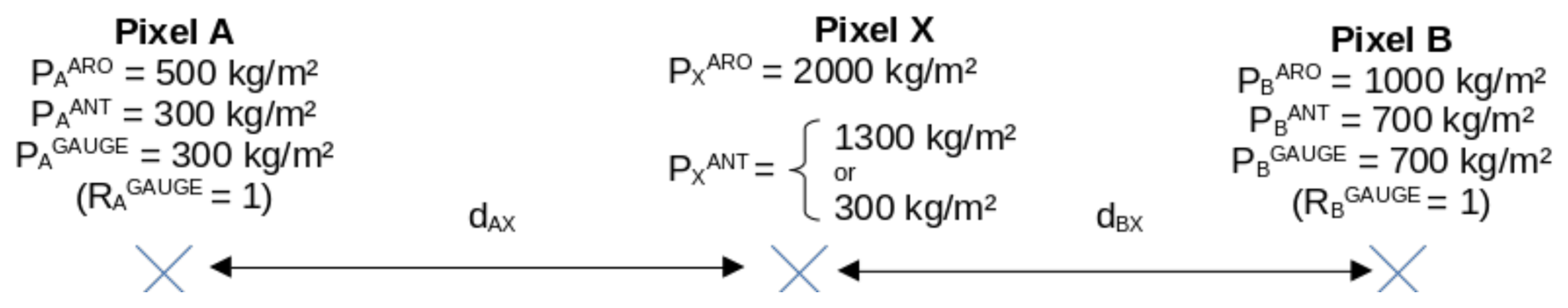
Figure A1 Illustration of the ANTILOPE climatological error estimation method on a pixel X with two available reference gauges (on pixels A and B).

Table A1 Values of the different steps of the error estimation method depending on the value of the yearly ANTILOPE precipitation accumulation on pixel X ($P_{\mathrm{X}}^{\mathrm{ANT}}$).

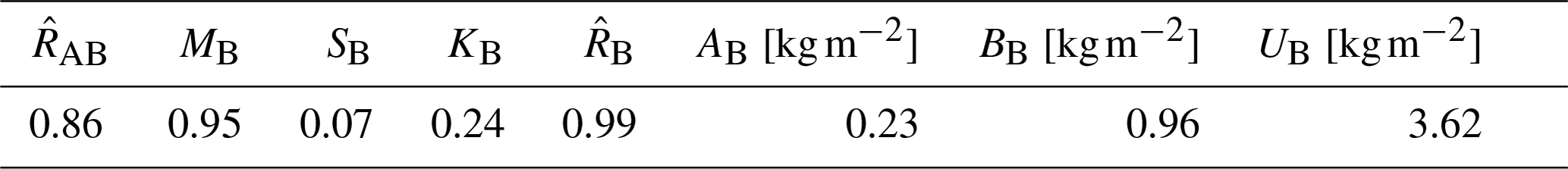
In order to complete the illustration, Tables A2 and A3 give the values of the different steps of the error estimation method applied to pixels A and B benefiting from gauge measurements. It is assumed that pixels A and B are 10 km apart (d_AB=10 km and $w_{\mathrm{AB}}=w_{\mathrm{BA}}=\mathrm{0.5}$). Since the precipitation ratios between pixels A and B are different for AROME and ANTILOPE, the estimated ratios ${\widehat{R}}_{\mathrm{BA}}$ and ${\widehat{R}}_{\mathrm{AB}}$ are significantly different from 1 (1.17 and 0.86 respectively). However, the inverse distance weighting ensures that the ultimate value of the estimated ratios ${\widehat{R}}_{\mathrm{A}}$ and ${\widehat{R}}_{\mathrm{B}}$ does not significantly differ from the actual ANTILOPE$/$GAUGE ratios $R_{\mathrm{A}}^{\mathrm{GAUGE}}$ and $R_{\mathrm{B}}^{\mathrm{GAUGE}}$ (1.01 and 0.99 respectively). Similarly, the estimated uncertainty remains minimal for each pixel (3.61 and 3.62 kg m⁻² respectively) thanks to the presence of a reference gauge with an identical climatology.

Table A2 Values of the different steps of the error estimation method applied to pixel A when d_AB=10 km.

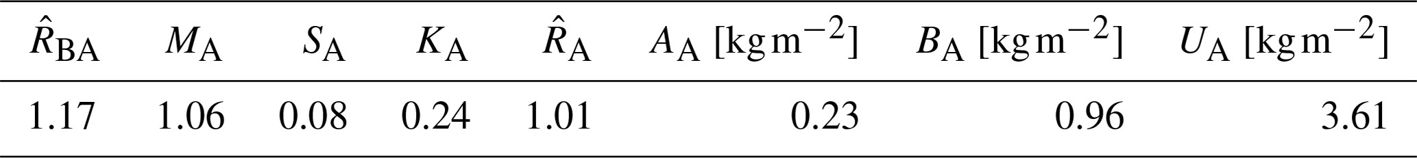
Table A3 Values of the different steps of the error estimation method applied to pixel B when d_BA=10 km.

Appendix B: Evaluation scores

The Brier score (BS) assesses the ability of an ensemble to forecast a threshold being exceeded. For each given event k, the predicted probability y_k of a given threshold being exceeded (the number of members forecasting the event divided by the size of the ensemble) is compared with the corresponding binary observation o_k of the threshold being exceeded, and for N events the BS is given by

$$\begin{array}{}\text{(B1)}& \mathrm{BS}={\displaystyle \frac{\mathrm{1}}{N}}\sum _{k=\mathrm{1}}^N{\left(y_k-o_k\right)}^{\mathrm{2}}.\end{array}$$

Although the BS was originally designed for ensemble systems, it is also commonly used in a deterministic context (DeMaria et al., 2009; Vernay et al., 2015), where the predicted probability y_k only takes values of 0 and 1. The Brier score ranges from 0 to 1, with 0 corresponding to a perfect score. It is computed for different precipitation thresholds from 1 to 30 kg m⁻² to check the ability of each product to forecast a variety of precipitation events.

The continuous ranked probability score (CRPS; Matheson and Winkler, 1976) is a measure of the difference between the ensemble cumulative distribution function F_y predicted for a given event and the Heaviside function centred on the associated observation H_o:

$$\begin{array}{}\text{(B2)}& \mathrm{CRPS}=\underset{\mathbb{R}}{\int }{\left(F_y\left(z\right)-H_{\mathrm{o}}\left(z\right)\right)}^{\mathrm{2}}\mathrm{d}z.\end{array}$$

Unlike the ensemble mean bias, the CRPS takes into account the error of each member of the ensemble: an unbiased ensemble with a large spread can have a higher CRPS than a slightly biased ensemble with a small spread.

Appendix C: Additional results

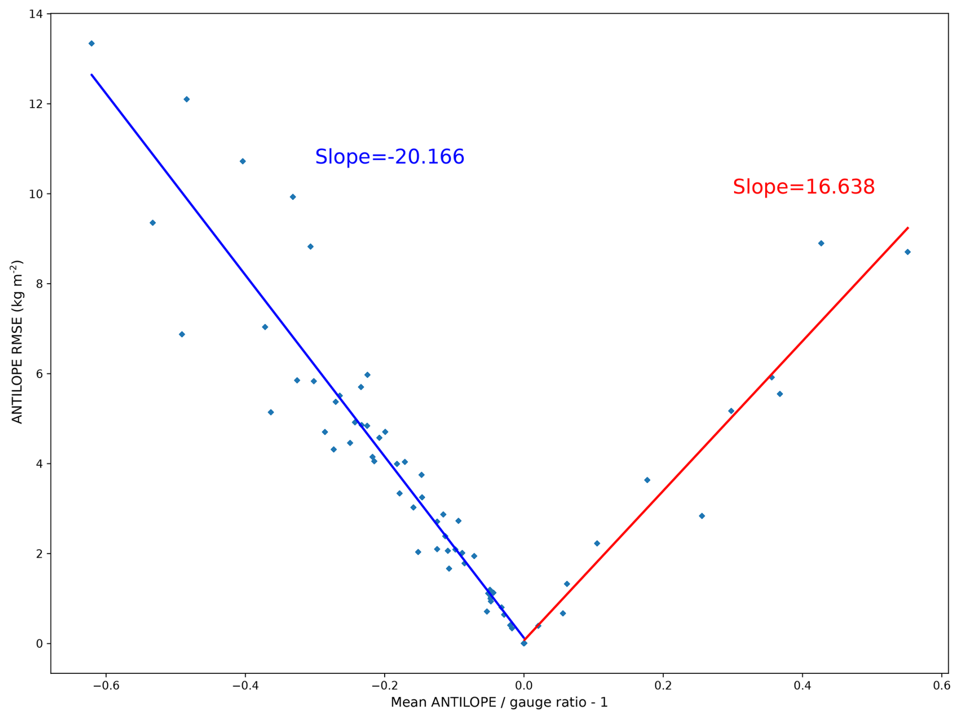
Figure C1 Linear regression between ANTILOPE$/$gauge mean ratio (R^GAUGE−1) and the corresponding RMSE over the 68 reference stations. The slope coefficients are used in the method described in Sect. 3.1.1.

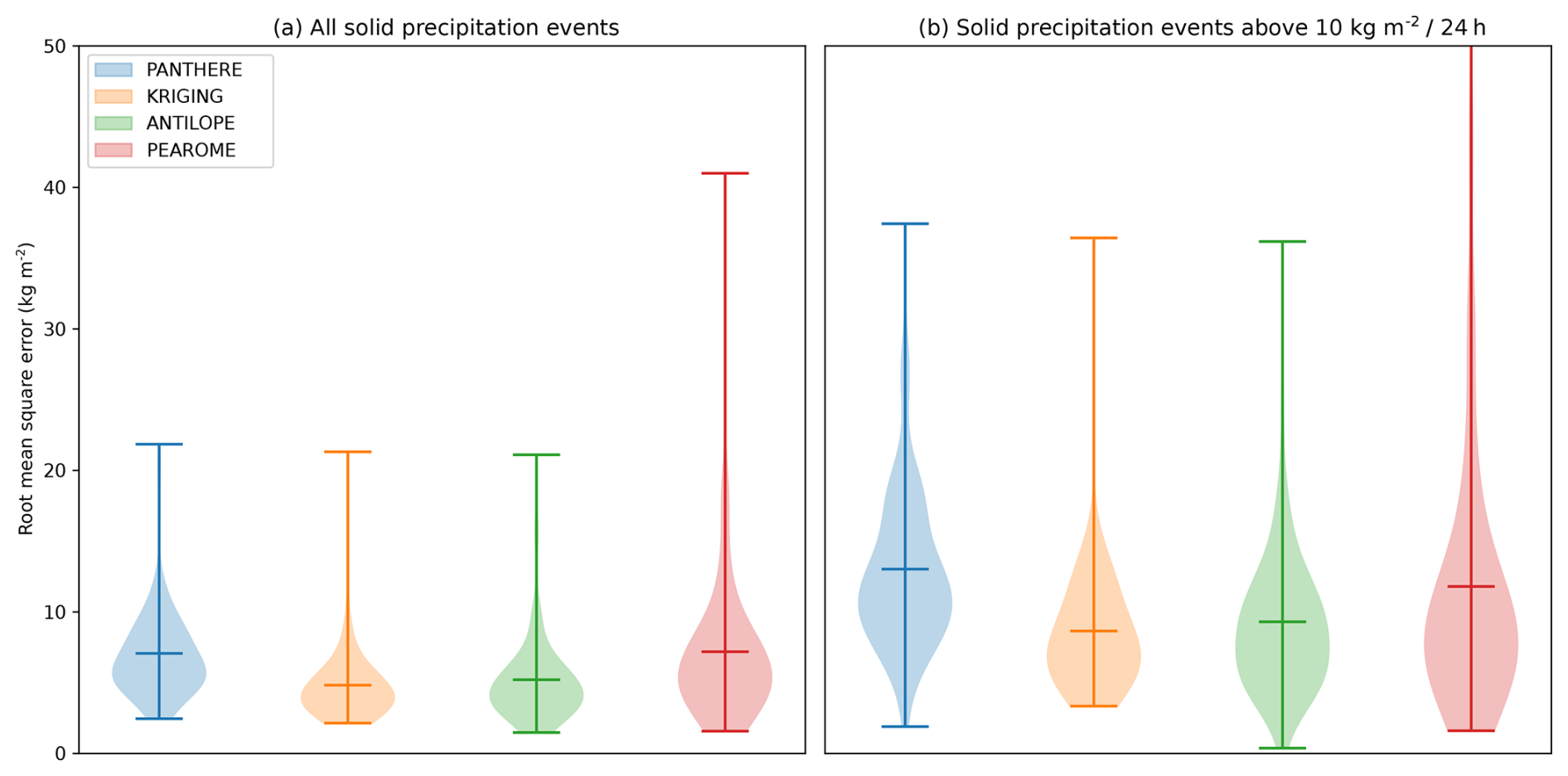
Figure C2 Same as Fig. 6 but considering only snowfall events. The precipitation phase is determined by the additional ski-resort observation of the maximum altitude reached by rain during the observation period. Only situations where this maximum altitude is below the station altitude are considered here.

Appendix D: Ensemble precipitation analyses

Figure D1 Raw post-processed PEAROME ensemble 24 h precipitation fields of 4 December 2021, downscaled to the ANTILOPE 1 km resolution over the Mont Blanc area (see Fig. 1). The corresponding raw ANTILOPE observation and the associated pre-processed fields are shown in Fig. 11.

Figure D2 The 24 h ensemble precipitation analysis of 4 December 2021 over the Mont Blanc area (see Fig. 1) obtained by a random sampling around the pre-processed ANTILOPE field (Sect. 3.2.1). The corresponding raw ANTILOPE observation and the associated pre-processed fields are shown in Fig. 11.

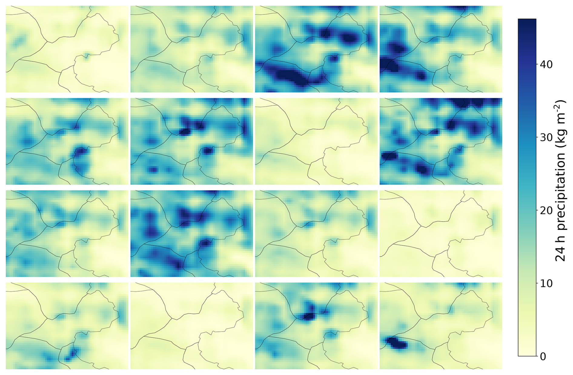
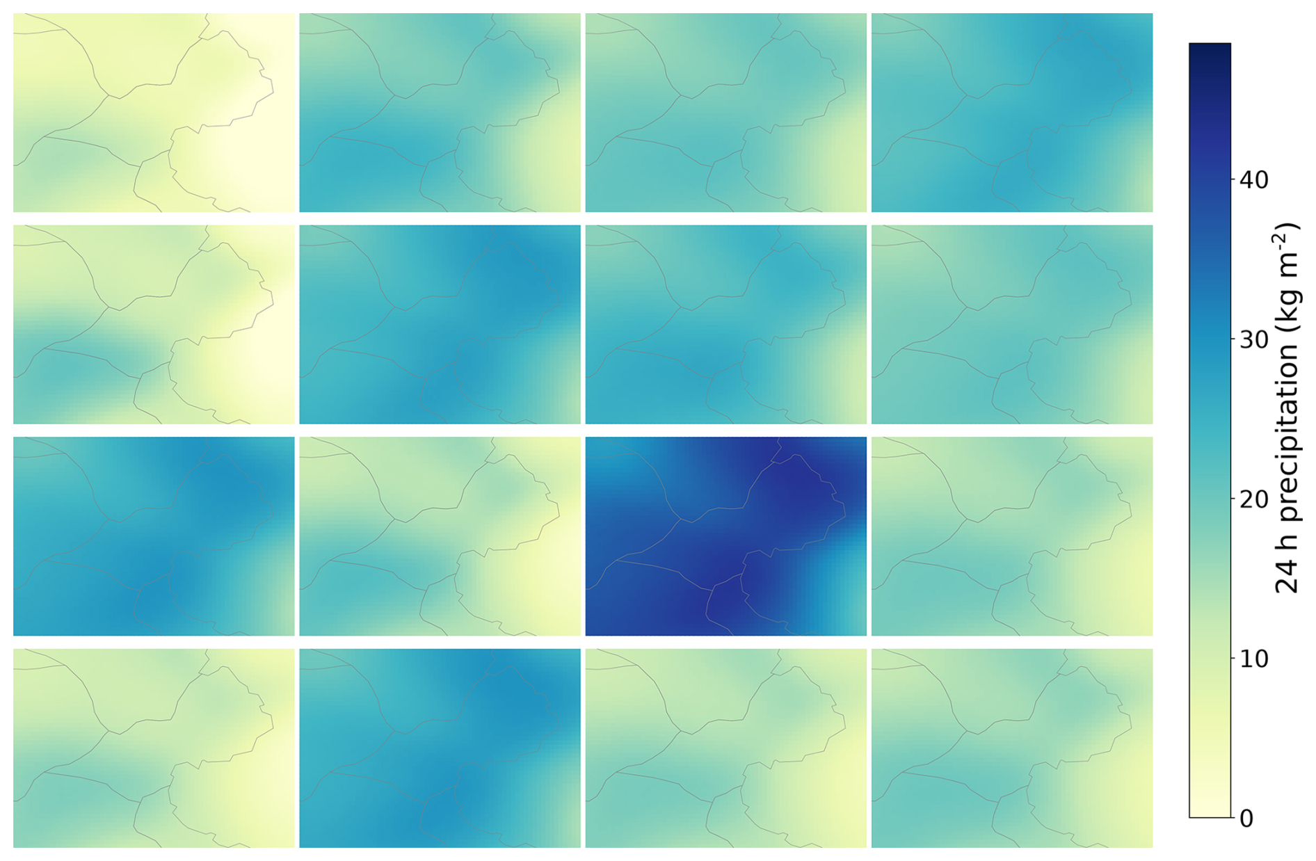
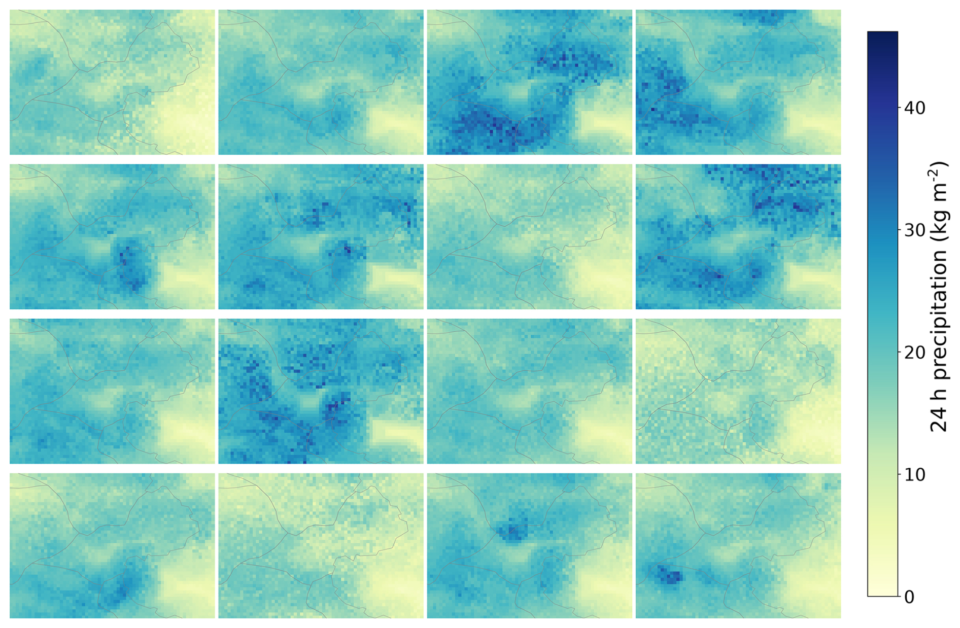
Figure D3 The 24 h ensemble precipitation analysis of 4 December 2021 over the Mont Blanc area (see Fig. 1) obtained with the particle filter method (Sect. 3.2.2). The corresponding raw ANTILOPE observation and the associated pre-processed fields are shown in Fig. 11, and the post-processed PEAROME ensemble is shown in Fig. D1.

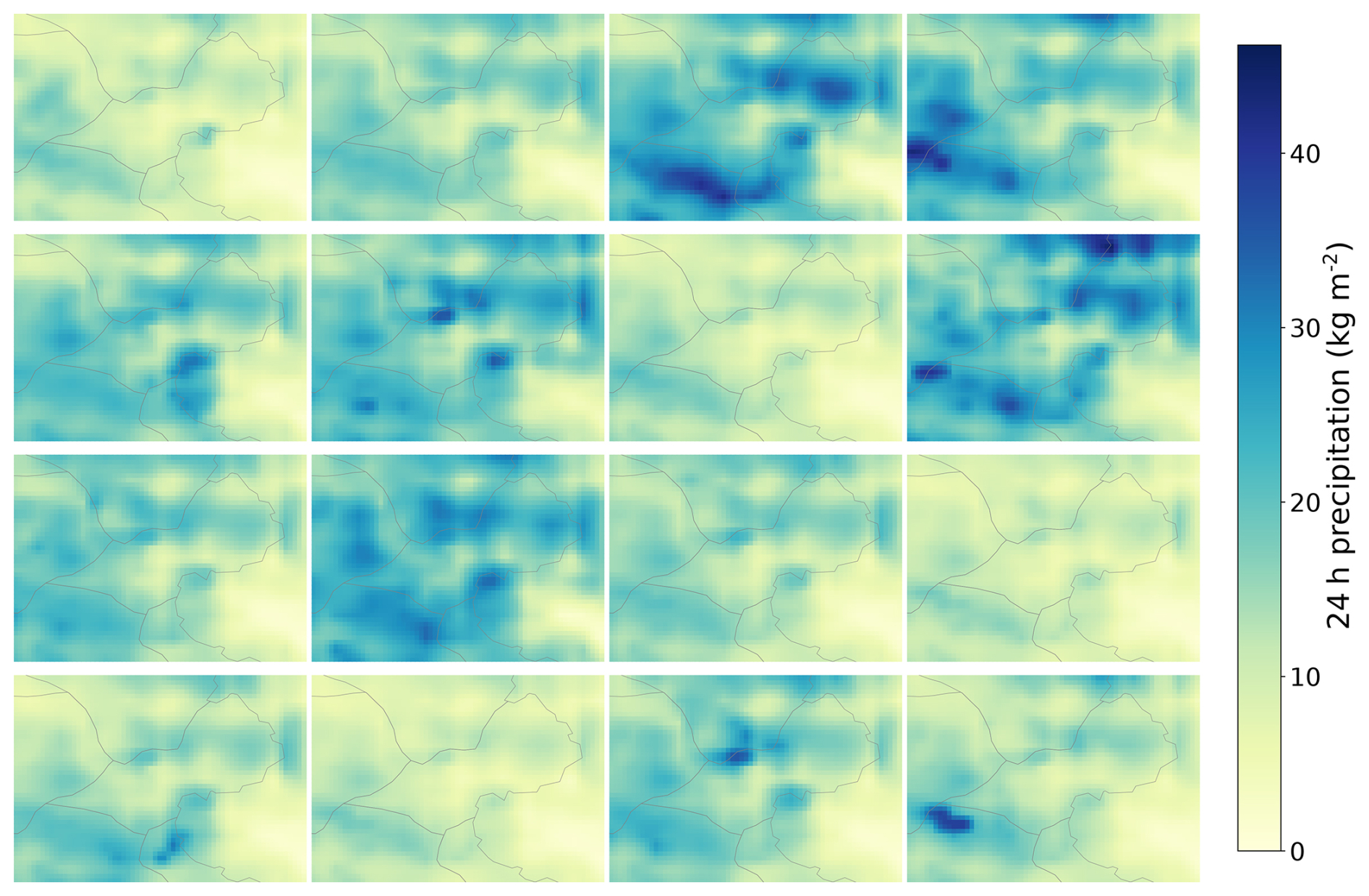
Figure D4 The 24 h ensemble precipitation analysis of 4 December 2021 over the Mont Blanc area (see Fig. 1) obtained with the ensemble Kalman filter method (Sect. 3.2.3). The corresponding raw ANTILOPE observation and the associated pre-processed fields are shown in Fig. 11, and the post-processed PEAROME ensemble is shown in Fig. D1.