Gridded surface O₃, NO_x, and CO abundances for model metrics from the South Korean ground station network

We present gridded surface air quality datasets over South Korea for three key species – ozone (O₃), carbon monoxide (CO), and nitrogen oxides (NO_x) – during the time frame of the Korea–US Air Quality (KORUS-AQ) mission (May–June 2016). Mixing ratios for the key species were mapped to 0.1° × 0.1° grid cells (hourly resolution), which were constructed from the 300+ air quality network sites using inverse distance weighting with simple declustering. Cross-comparing the interpolated fields against the site data that were used to create them reveals high prediction skill for O₃ (80 %) throughout South Korea and moderate skill (60 %) for CO and NO_x on average in densely observed regions after individual mean bias corrections. The gridded O₃ and CO interpolations predict the NASA DC-8 observations in the planetary boundary layer (PBL) with high skill (80 %) in the Seoul Metropolitan Area (SMA) after subtracting the mean bias. DC-8 NO_x observations were much less predictable on account of consistently negative vertical gradients within the PBL. Our gridded products capture the mean of and variability in O₃ throughout South Korea and the mean of and variability in CO and surface NO_x in most site-dense urban centres (SMA, Cheongju, Gwangju, Daegu, Changwon, and Busan).

1 Introduction

Air quality control has become a priority in the Republic of Korea following an upward trend in ozone (O₃) pollution in all major cities since the 1980s (Susaya et al., 2013). In May–June 2016, the Korea–US Air Quality (KORUS-AQ) mission was launched with the goal of improving knowledge of the factors controlling South Korean air pollution; this mission gathered extensive observational data via aircraft, ground stations, ships, and remote sensing (Crawford et al., 2021).

Comparisons of modelled grid-cell values (i.e. averages) with point data from station sites remain awkward, especially in high-emission environments with high sub-grid and temporal variability. Ground site comparisons in South Korea have thus far used the arithmetic mean of sites within a grid cell or ungridded quantile analysis (Lennartson et al., 2018; Peterson et al., 2019; Eck et al., 2020; Jordan et al., 2020; Schroeder et al., 2020; Park et al., 2021; Oak et al., 2022; Travis et al., 2022), but these unweighted means can be biased by site clustering, and they lose information outside the cells. In this work we develop a gridded dataset of key surface-level pollutants (in this case, O₃, NO_x, CO) observed during the KORUS-AQ time frame. In contrast to arithmetic means, we apply inverse distance weighting (IDW) interpolations (Shepard, 1968) improved by Schnell et al. (2014) to create country-wide continuous mapping of the National Institute of Environmental Research (NIER) ground site data. We subsequently integrate the interpolated field over a 0.1° × 0.1° grid. To evaluate the interpolation, we predict NIER station measurements using the leave-one-out cross-validation method; we predict observations from two research sites (Olympic Park and Taehwa Forest) to verify instrumental cohesion, and we compare our gridded fields with DC-8 observations within the planetary boundary layer (PBL) to gauge how well the data products reproduce upper PBL abundances. In addition to providing gridded PBL datasets, we discuss the applicability and limitations of our methodology for each key species.

The observational datasets are described in Sect. 2 and the methods in Sect. 3. Results are summarized in Sect. 4. Conclusions and recommendations are presented in Sect. 5.

2 KORUS-AQ data

All KORUS-AQ datasets introduced in this section including the raw 5 min NIER station data are available via https://doi.org/10.5067/Suborbital/KORUSAQ/DATA01 (KORUS-AQ Science Team, 2019). The NIER station data are access-controlled, but we record our processed hourly averaged NIER station data and our quality control flags for the raw data in our repository (see Wilson, 2025).

2.1 NIER air quality stations

The AirKorea monitoring network (https://www.airkorea.or.kr/eng, last access: 4 January 2025) provided ground measurements of the key species averaged every 5 min at 323 stations across South Korea, of which 319 reported O₃, 311 reported CO, and 321 reported NO_x (Fig. 1). We calculate hourly median readings centred on the hour for each station but omit clearly erroneous O₃ and NO_x dropouts from the average. High outliers exceeding 5 standard deviations above the mean of a weekly period were also discarded along with dropouts, which were manifest as stably low concentrations (1–4 ppb) persisting for multiple hours in stark contrast with the typical variability at the site. We were able to flag most dropouts algorithmically by analysing the cumulative density functions (CDFs) of the station data partitioned into non-overlapping weekly intervals; improbably low frequency data often featured flat empirical gradients (less than 100th of the median CDF gradient) at the tail of the CDF. This technique proved insufficient at some stations however, and so we manually removed dropouts that were not flagged by our algorithm, as did Eck et al. (2020). The NIER instruments and procedures are not well documented, and there remain some oddities: CO was reported with 1 ppb precision at 68 sites and with 100 ppb precision at the remaining 250 sites.

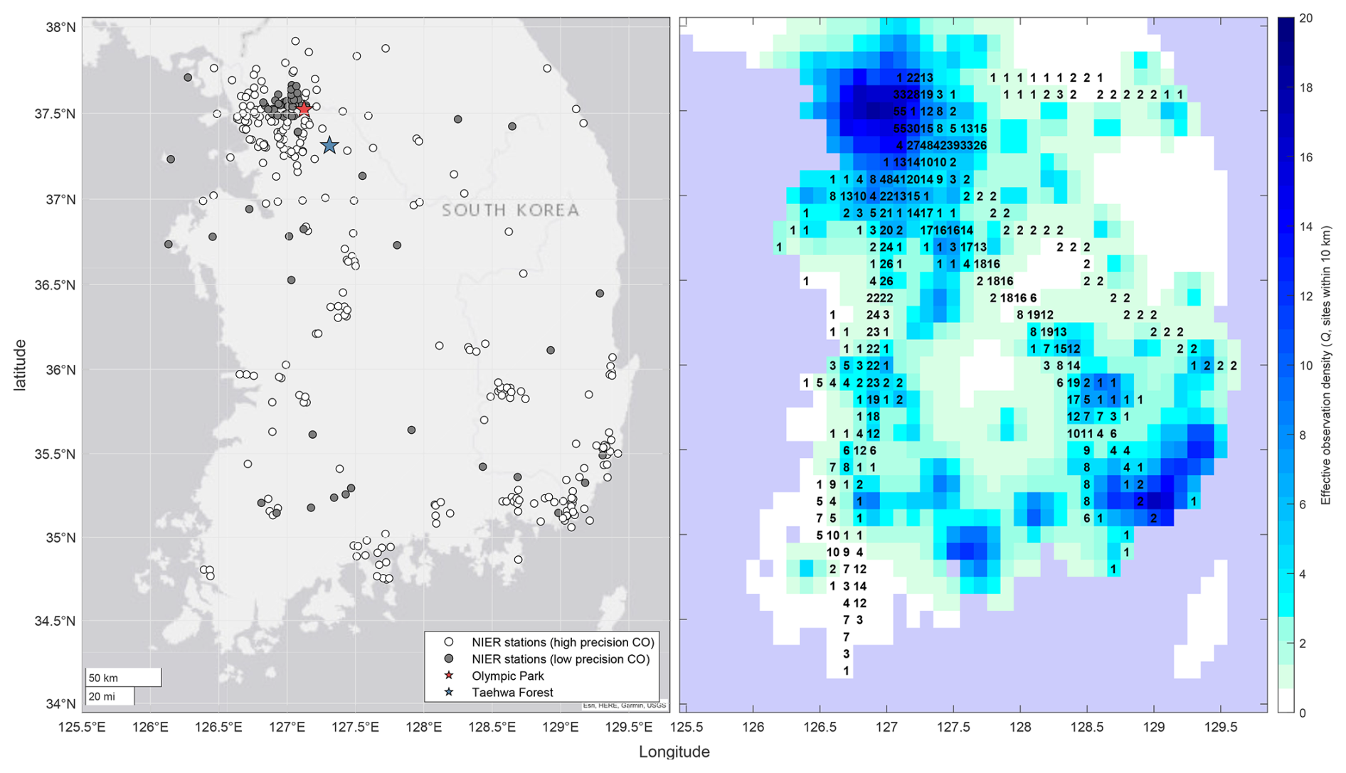
Figure 1 Left: the geographical distribution of NIER ground stations and the two surface research stations operating during the KORUS-AQ campaign. High-precision stations (white circles) recorded CO at 1 ppb precision; low-precision stations (grey circles) recorded CO at 100 ppb increments. Right: effective NIER station density (colour) within a 10 km radius (Q; see Eq. 3) gridded over 0.1° × 0.1° cells. The number of contiguous DC-8 flight transects through each box in the PBL is printed in each cell. The aircraft radar altitude was evaluated against the ERA5 PBL height (based on hourly 0.25° × 0.25° gridded data; Hersbach et al., 2023). The ERA5 data were interpolated in time to match the aircraft data.

2.2 Research stations

2.2.1 Olympic Park

The Olympic Park research station lies at the southeast edge of Seoul at 37.5216° N, 127.1242° E, 30 m above sea level, and served as a reference for ground-level Seoul pollution during the KORUS-AQ campaign (red star in Fig. 1). Hourly averages for the key species were recorded using Ecotech EC9841 NO_x, Ecotech EC9830 CO, and Ecotech EC9810 O₃ instruments (PI: Cho Seogu) during the KORUS-AQ period (10 May 01:00:00 to 18 June 00:00:00 LT). As the Olympic Park station has four proximal NIER stations within 5 km, reproducing this research station data from the NIER interpolation should be a test of the small-scale variability in Seoul pollution provided the instruments are well calibrated.

2.2.2 Taehwa Forest

The Taehwa Forest wilderness site lies 30 km southeast of Olympic Park at 37.3123° N, 127.3105° E, at 200 m elevation (blue star in Fig. 1). It was used primarily to investigate the mixing of urban Seoul pollution with the biogenic volatile organic compounds (BVOCs) of the forest. The three key species were measured by the existing NIER instruments (PI: Youngjae Li) but supplemented by a Thermo Scientific 42i instrument for NO and a cavity ring-down spectroscopy instrument for NO₂ (PI: Kim Saewung; Kim et al., 2022).

2.3 NASA DC-8

The DC-8 aircraft routinely profiled the air over Taehwa Forest via loop manoeuvres in the morning and afternoon on flight days between 2 May and 11 June 2016. It sampled other regions above South Korea and the Yellow Sea according to pollution plume transport and cloud forecasts. We use the 10 s merged data of our three key species. O₃ and NO_x (NO and NO₂) were measured with a four-channel chemiluminescence instrument (Weinheimer et al., 1994), and CO was measured by the Differential Absorption CO Measurement (DACOM) instrument (Sachse et al., 1991). We also use the 10 s data for latitude, longitude, radar altitude, UTC time, and potential temperature (PI: Melissa Yang). From the DC-8 potential temperature measurements and ERA5 surface data (Fig. A1), we can show that the ERA5 PBL heights accurately select DC-8 observations that are adiabatically mixed from the surface (i.e. $\mathrm{d}\mathit{\theta }/\mathrm{d}z$ ∼ 0), which is confirmed by the afternoon O₃ and CO profiles (Fig. A2). To determine when the aircraft was in the PBL and thus could be compared with the interpolated surface map, we use the ERA5 PBL height data from reanalysis (hourly, 0.25° × 0.25° grid; Hersbach et al., 2023). This approach is more accurate than simply assuming that all DC-8 observations below 1.5 km radar altitude fall within the PBL (e.g. Oak et al., 2019).

3 Methods

Interpolation techniques compute an objective estimate $Z^{\prime }(x,t)$ of a field Z(x,t) at any geographic location x and time t as a weighted mean of observations Z_k(t) at stations indexed by k with weights w_k(x):

$$\begin{array}{}\text{(1)}& Z^{\prime }\left(x,t\right)={\sum }_k\left[w_k\left(x\right)Z_k\left(t\right)\right]/{\sum }_k{w}_k\left(x\right).\end{array}$$

Ordinary kriging and inverse distance weighting (IDW) are two common interpolation methods that operate by this premise but differ in how the station weights (w_k) are calculated (Matheron, 1963; Shepard, 1968). Kriging is a family of statistical techniques based on the supposition that phenomena are autocorrelated in space, relying on an empirical distance-based covariance model of Z(x,t) determined from the station data. In our work we find minimal Pearson's correlation between pairwise site covariance and proximity for any of the key species, so we opt for the modified IDW approach of Schnell et al. (2014).

We examine the autocovariance functions of the sites to characterize the temporal variability in each key species at 5 min resolution. The autocovariance function for a given phase shift (e.g. 10 min) is defined as the covariance of a time series of data with itself but phase-shifted by 10 min. The O₃ site autocovariance functions feature strong diurnal cycles, preserving on average half of the respective site variances for a 24 h phase shift, compared with 35 % for CO and NO_x. Sub-10 min variability accounts for 3 % of the O₃ site variance and 12 % of the CO and NO_x variance on average. Heterogeneous emissions and micrometeorology may be attributed to some of the CO and NO_x short-timescale variability seen in some Seoul sites and many CO-measuring sites in the Gwangyang–Yeosu–Suncheon zone, while rural sites suggest a possible instrumental noise component of the NO_x variability (see Fig. B1 of Appendix B).

3.1 Inverse distance weighting

In IDW techniques, weights are calculated from the reciprocal distances between estimation point x and the station coordinates x_k, scaled by the exponent β. The greater density of observations in some regions creates a source of oversampling bias. Schnell et al. (2014) address this clustering effect by reducing all station weights by M_k, the number of other stations within distance D of site k, discounting sites with missing readings on an hourly basis. In order to smooth the spatial heterogeneity in $Z^{\prime }(x,t)$ at small length scales, the distance D also serves as the minimum cutoff of x−x_k and hence determines the maximum weighting w_k(x) of any nearby station. L is a maximum cutoff of x−x_k used to reduce excess calculations for extremely distant and unimportant sites. The weight formulae are summarized in Eq. (2):

$$\begin{array}{}\text{(2)}& \begin{array}{lcr}{w}_k\left(x\right)=\frac{D^{-\mathit{\beta }}}{M_k}& \text{for}& x-x_k\le D,\\ w_k\left(x\right)=\frac{{\left(x-x_k\right)}^{-\mathit{\beta }}}{M_k}& \text{for}& D<x-x_k\le L,\\ w_k\left(x\right)=\mathrm{0}& \text{for}& x-x_k>L.\end{array}\end{array}$$

Our NIER station data consist of $k\in \mathit{\{}\mathrm{1},\mathrm{2},\mathrm{\dots },\mathrm{323}\mathit{\}}$ locations (Fig. 1) and $t\in \mathit{\{}\mathrm{1},\mathrm{2},\mathrm{\dots },\mathrm{936}\mathit{\}}$ hourly observations (10 May 01:00:00 to 18 June 00:00:00 LT) for each of our three key species (O₃, CO, NO_x), with some unreported or erroneous data. We optimize β and D for each key species Z by randomly removing a fifth of the stations from the algorithm and then predicting the abundance at each missing station k^′, adjusting each parameter until a 2D minimum is reached. In minimizing the total root-mean-square error between predictions $Z_{k^{\prime }}^{\prime }\left(t\right)$ and observations $Z_{k^{\prime }}\left(t\right)$ over the time series, we find similar optimal values for each species (β ∼ 2, D ∼ 5 km, L ∼ 80 km), with no significant improvement for larger L values. The effective density of observations Q(x) is defined as the effective number of NIER sites within a 10 km radius of x in Eq. (3) (also called quality of prediction, Eq. 5 of Schnell et al., 2014). We expect Q to correlate with prediction accuracy:

$$\begin{array}{}\text{(3)}& Q\left(x\right)={\mathrm{10}}^{\mathit{\beta }}{\sum }_k{w}_k\left(x\right).\end{array}$$

Compared with the arithmetic mean gridding, the gridded IDW observations show no significant mean bias. However, significant mean absolute deviations can be seen in the densely observed (Q > 10) Seoul Metropolitan Area and southeast coastal cities. In such regions, the mean absolute deviations for O₃, CO, and NO_x are 5, 58, and 9 ppb, respectively. Conversely, the most sparsely measured regions show the best agreement between the two methods due to mutual sampling of a single station. Both methods are fundamentally limited by sampling density, particularly in urban centres with high spatial emission variability. The differences seen in the most densely observed regions highlight the instability of the arithmetic mean method with respect to grid size and boundary manipulation.

3.2 Statistical techniques

To evaluate the accuracy and predictive capability of an interpolation, we examine the error E(t) in a time series of predictions Pre(t) and observations Obs(t) at a given location for a given species with all time points equally weighted. We calculate a sequence of three error series defined as follows:

$$\begin{array}{}\text{(4)}& \begin{array}{l}E\mathrm{1}\left(t\right)=\text{Pre}\left(t\right)-\text{Obs}\left(t\right),\\ E\mathrm{2}\left(t\right)=\text{Pre}\left(t\right)-\text{Obs}\left(t\right)-(\stackrel{\mathrm{‾}}{\text{Pre}\left(t\right)}-\stackrel{\mathrm{‾}}{\text{Obs}\left(t\right)}),\\ E\mathrm{3}\left(t\right)=b\text{Pre}\left(t\right)-\text{Obs}\left(t\right)-(b\stackrel{\mathrm{‾}}{\text{Pre}\left(t\right)}-\stackrel{\mathrm{‾}}{\text{Obs}\left(t\right)}),\end{array}\end{array}$$

where E1(t) is the absolute error in the predictions; E2(t) is the error after correcting for the mean prediction bias $\left(\stackrel{\mathrm{‾}}{\text{Pre}\left(t\right)}-\stackrel{\mathrm{‾}}{\text{Obs}\left(t\right)}\right)$; and E3(t) is the error relative to a simple linear regression (LR) model of Pre(t) vs. Obs(t) fitted by ordinary least squares, i.e. after correcting for mean bias and slope (b). We then apply the coefficient of determination to compute the fraction of the observed sample variance, Var(Obs(t)), explained by, for example, the raw predictions (E1(t)):

$$\begin{array}{}\text{(5)}& R_{E\mathrm{1}}^{\mathrm{2}}=\mathrm{1}-{\displaystyle \frac{\text{mean}\left(E\mathrm{1}(t{)}^{\mathrm{2}}\right)}{\text{Var}\left(\text{Obs}\left(t\right)\right)}}.\end{array}$$

And we do similarly for E2(t) and E3(t). $R_{E\mathrm{1}}^{\mathrm{2}}$ is a predictive accuracy statistic that ranges from minus infinity to 1 and is identical to the forecast skill score referenced to the mean of observations (Murphy, 1988). $R_{E\mathrm{2}}^{\mathrm{2}}$ describes how well the predictions capture the temporal variability in the observations regardless of any mean bias and has the same range as $R_{E\mathrm{1}}^{\mathrm{2}}$. $R_{E\mathrm{3}}^{\mathrm{2}}$ is the common definition of R² in regression analysis and ranges from zero to 1 due to the fitting constraint. $R_{E\mathrm{3}}^{\mathrm{2}}$ describes the predictability of the observations from the LR model regardless of any difference in the mean or variance of Pre(t) and Obs(t). A score of zero for a given $R_E^{\mathrm{2}}$ is equivalent to predicting a static mean of observations across the time domain. The maximum score for $R_{E\mathrm{1}}^{\mathrm{2}}$ and $R_{E\mathrm{2}}^{\mathrm{2}}$ is limited by the interpolation variance, which is typically damped relative to the contributing stations, especially in regions with highly heterogeneous emissions. Figure 2 (right-hand side) suggests the average station predictability ($R_{E\mathrm{1}}^{\mathrm{2}}$ and $R_{E\mathrm{2}}^{\mathrm{2}}$) score has an upper bound of around 0.9 for O₃ and 0.8 for CO and NO_x.

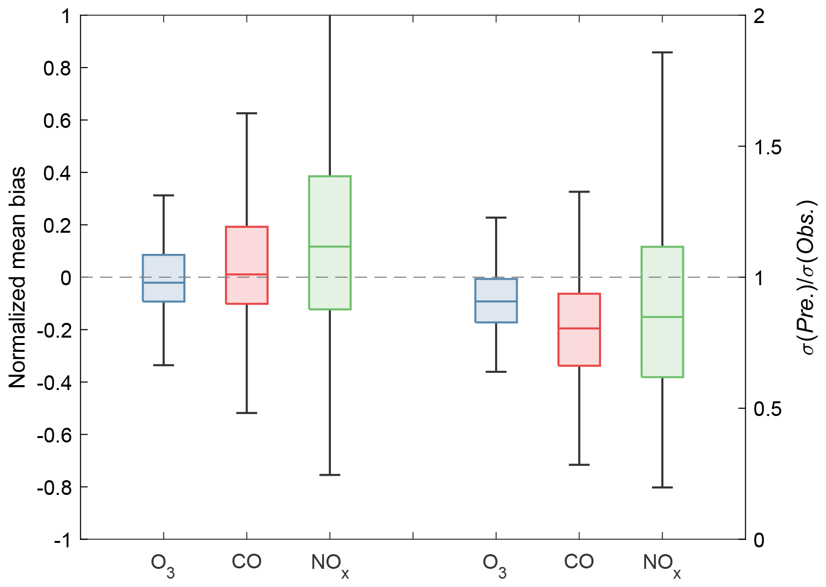
Figure 2 Left: box plots of normalized mean bias: $\text{NMB}\left(k\right)=\text{mean}\left(\text{Pre}\left(k,t\right)-\text{Obs}(k,t)\right)/\text{mean}\left(\text{Obs}\right(k,t\left)\right)$. Right: standard deviation ratio $\mathit{\sigma }\left(\text{Pre}(k,t)\right)/\mathit{\sigma }\left(\text{Obs}(k,t)\right)$ for interpolated time series at each NIER site using leave-one-out cross-validation. Whiskers show the range of non-outliers, where outliers are data beyond 1.5 interquartile ranges from the outer quartiles. Results are shown for O₃ (blue), CO (red), and NO_x (green). Mean bias is normalized by the observed mean, and the ratio of standard deviations is analogous to the gradient of a linear regression.

Leave-one-out cross-validation

In this trial, we sequentially remove each station k and then interpolate (predict) its value from the remaining stations: $\text{Pre}(k,t)=Z^{\prime }(k,t)$, where $\text{Obs}(k,t)=Z(k,t)$ (see Eq. 4; Brauer et al., 2003; Hochadel et al., 2006). A perfect interpolation would accurately reproduce the mean and standard deviation of the measurements, indicating (1) no mean bias error and (2) preservation of daily maxima and minima. Our optimized IDW interpolation has clearly worked well in terms of mean bias (left half of Fig. 2). The box quartiles and non-outlier whiskers (i.e. the full range of values within one-and-a-half 1.5 interquartile ranges from the outer quartiles) are well centred on zero bias, with the spread broadening from O₃ to CO to NO_x. The symmetry of the whiskers comes from the case where two sites, distant from the remaining sites but near one another, are the only sites used to interpolate one another, and hence if one site has twice the mean value of another, we get symmetric plus–minus biases for each site. The median of the mean NO_x site biases is +13 %, and this appears to be an artefact of low NO_x abundances in rural (Q < 5) locations. The absolute mean NO_x bias averages −0.6 ppb (urban −3.0 ppb, rural +6.5 ppb). Incoherence among nearby urban stations combines to dampen the interpolation variability, especially for CO and NO_x, which feature independent high spatial variability from local sources. This is shown on the right half of Fig. 2, where most of the standard deviation ratio quantiles lie below unity. We believe this reduced standard deviation in the prediction time series better represents the average over a grid cell that contains several incoherent sites.

The sequences of $R_E^{\mathrm{2}}$ scores (E1–E3) for each site and each species are shown in Fig. 3. The O₃ scores (top row) are consistently high across the sequence. Scores of $R_{E\mathrm{1}}^{\mathrm{2}}$ through $R_{E\mathrm{3}}^{\mathrm{2}}$ for O₃ indicate that the O₃ interpolation was accurate and unbiased at almost all NIER stations in South Korea. For CO (middle row) and NO_x (bottom row), there is an improvement in absolute prediction accuracy ($R_{E\mathrm{1}}^{\mathrm{2}}$) as the density of observations (Q) increases and further improvement after correcting the mean bias in the predictions ($R_{E\mathrm{2}}^{\mathrm{2}}$). The linear regression models ($R_{E\mathrm{3}}^{\mathrm{2}}$) offer an obvious improvement to predictability in rural regions (low Q) where information is lacking but no significant improvement in well-sampled urban regions (high Q). With no large net mean bias for any key species (Fig. 2), we assert that the average of our interpolations should capture the mean of and possibly the variability in a well-mixed gridded domain. We test this assertion later using aircraft PBL observations averaged into 0.1° × 0.1° cells. The high range of $R_E^{\mathrm{2}}$ values for NO_x and CO, even where Q > 10, suggests that absolute mean error in the prediction is a problem for many sites, implying they are driven by very small scale (< 1 km) local emissions in contrast to O₃, which is not emitted directly. For NO_x, the sequence from E1 to E2 greatly improves the prediction accuracy. For CO, there remains a large fraction of unpredictable sites, often with very high standard deviations (dark-red circles), implying large nearby emissions. Figure 4 (top-middle and top-right panels) shows the clustering of such sites for CO and NO_x in Daejeon (central–western South Korea) and in the southern coastal cities of Gwangyang, Yeosu, Suncheon, Jinju, and Ulsan (no NO_x data). When we compare the leave-one-out cross-validation (LOOCV) performance of NO_x with the complete interpolation (i.e. no stations omitted; see bottom panel of Fig. 4), we see $R_{E\mathrm{2}}^{\mathrm{2}}$ scores change by > 0.4 at, for example, rural sites, the Busan shoreline, and the manufacturing district sites of northern Yeosu and eastern Gwangyang. These discrepancies indicate undersampling of NO_x across rural South Korea and in some urban districts with locally contrasting emission activity.

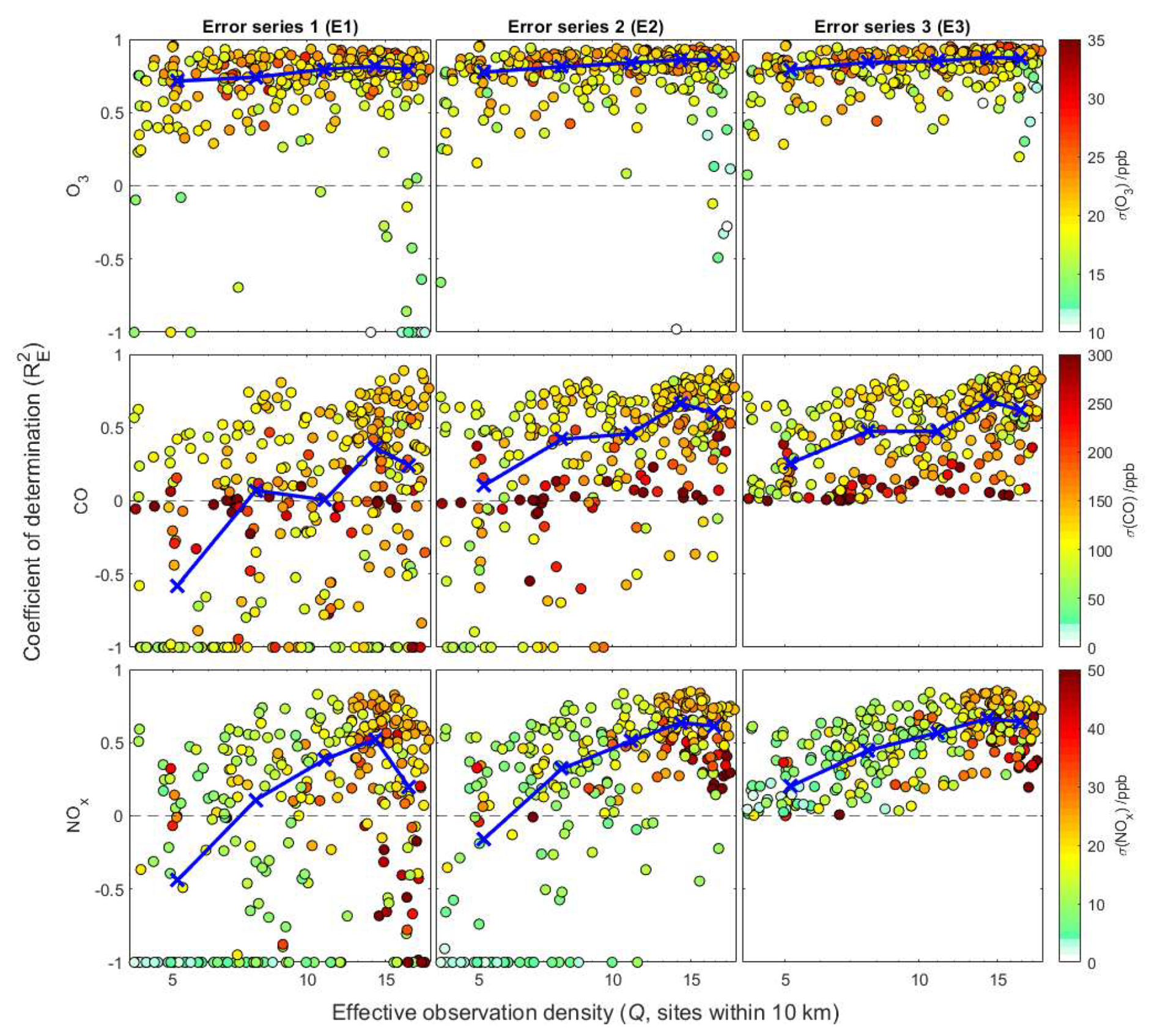
Figure 3 Generalized coefficient of determinations ($R_E^{\mathrm{2}}$, Eq. 5) for NIER station predictions vs. the effective density of nearby observations (Q, effective number of sites in a 10 km radius). The three columns show the sequence $R_{E\mathrm{1}}^{\mathrm{2}}$, $R_{E\mathrm{2}}^{\mathrm{2}}$, and $R_{E\mathrm{3}}^{\mathrm{2}}$. The three rows are for the species O₃ (top), CO (middle), and NO_x (bottom). The calculations use the leave-one-out cross-validation method at each NIER station (circles) coloured by the standard deviation of observations. The connected blue crosses show the median $R_E^{\mathrm{2}}$ values for five percentile partitions of Q: 0 %–20 %, 20 %–40 %, 40 %–60 %, 60 %–80 %, and 80 %–100 %.

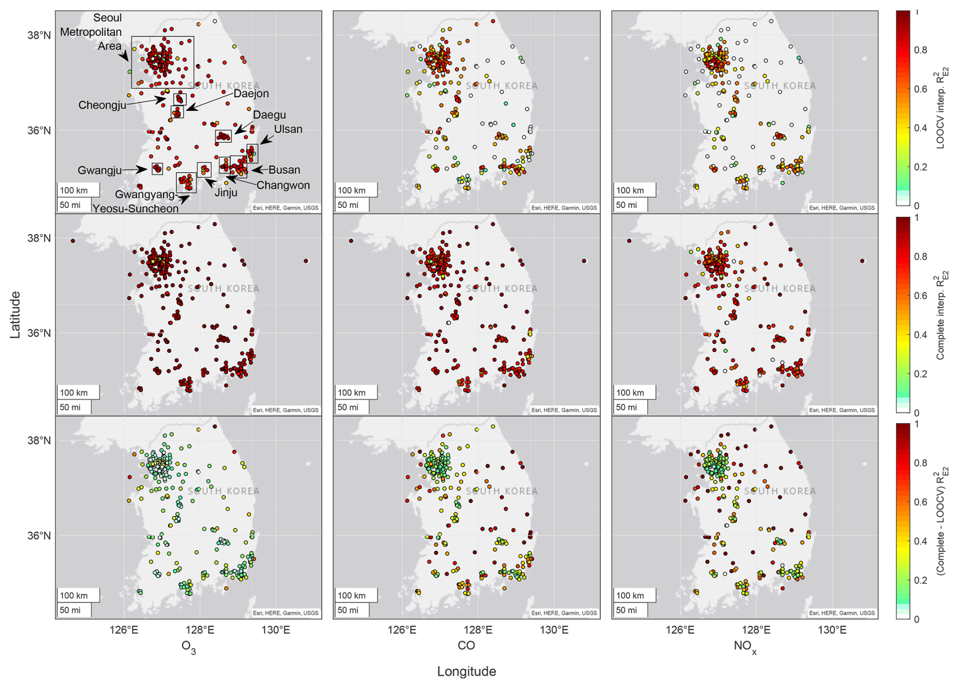
Figure 4 The geographical distribution of NIER station prediction accuracies with the mean prediction bias removed from each station ($R_{E\mathrm{2}}^{\mathrm{2}}$, Eqs. 4 and 5), shown for the three key species: O₃ (left), CO (middle), and NO_x (right). Top: $R_{E\mathrm{2}}^{\mathrm{2}}$ scores for the LOOCV interpolations. Middle: $R_{E\mathrm{2}}^{\mathrm{2}}$ scores for the complete interpolation, i.e. without omitting the data from predicted sites. Bottom: the difference between the complete and LOOCV interpolation $R_{E\mathrm{2}}^{\mathrm{2}}$ scores. Negative $R_{E\mathrm{2}}^{\mathrm{2}}$ values are truncated to zero. Approximate city bounds are shown via text and boxes in the top-left panel.

We have additionally compared the interpolation accuracy during the four meteorological phases presented by Peterson et al. (2019), i.e. dynamic, anticyclone, low-level transport, and Rex blocking, although we did not identify any obvious patterns across the phases (see Fig. C1 of Appendix C). An alternative test of meteorological influence is daytime (07:00 to 20:00 LT) vs. nighttime (21:00 to 06:00 LT) predictability, i.e. prevailingly turbulent vs. stably stratified atmospheric surface conditions. Ozone and NO_x, but not CO, showed greater LOOCV predictability ($R_{E\mathrm{2}}^{\mathrm{2}}$) during the daytime than nighttime by around +0.1 and +0.05, respectively (see Fig. C2). More efficient turbulent mixing during daytime vs. nighttime likely smoothed some of the small-scale emission heterogeneity, resulting in more predictable fields.

3.3 Gridded air quality data

A major objective of this study was to obtain grid-cell averages (0.1° × 0.1°, approx. 10 km × 10 km) for testing regional air quality models. Within each 0.1° × 0.1° cell, we interpolate the key species to 25 points on a 0.02° × 0.02° grid centred in the cell and then average these values. The averages do not account for latitudinal differences in quadrangle areas, which are minor for South Korean latitudes. We apply the same treatment to the density of observations to produce the gridded Q values as seen in Fig. 1 (right-hand side).

3.4 Aircraft cell averages

We collect the measurements of O₃, CO, and NO_x from NASA DC-8 taken over land at radar altitudes below the PBL heights taken from the ERA5 data. The DC-8 measurements used here are 10 s merged measurements corresponding to approximately 1 km flight segments $S\in \mathit{\{}\mathrm{1},\mathrm{2},\mathrm{\dots },\mathrm{13}\mathrm{942}\mathit{\}}$. To compare the segments with the gridded site data, we average the contiguous segments through each grid cell to produce transect-averaged observations Obs(T), where transects $T\in \mathit{\{}\mathrm{1},\mathrm{2},\mathrm{\dots },\mathrm{2106}\mathit{\}}$ contain around seven segments whose midpoints lie in the cell bounds. For the prediction set Pre(T), we interpolate the traversed cells in time to match the mean aircraft time of flight during the respective transects. The number of transects through each cell is indicated by the gridded numbers in Fig. 1 (right-hand side).

4 Results

4.1 Research site prediction

Research stations provide case studies where the quality of measurements is carefully controlled, and so instrumental drift, noise, and biases are minimized. For each key species, we compare the NIER station data interpolated to the coordinates of the research stations, at either Olympic Park or Taehwa Forest, against the research station instruments (Fig. 5). Olympic Park and Taehwa Forest have effective sampling densities (Q) of 16 and 6 stations per 10 km, respectively. Figure 5 shows accurate prediction of O₃ at both sites with predictably more scatter at Taehwa Forest, where less information was available. We see a similar pattern for CO but with a mean bias (predicted NIER interpolated value minus research instrument measurement) of +100 ppb at Taehwa Forest. NO_x is predicted reasonably well at Olympic Park except in the highest measured range (> 100 ppb), but predictions appear random at Taehwa Forest. Table 1 indicates excellent prediction accuracy at Olympic Park for all species ($R_{E\mathrm{1}}^{\mathrm{2}}$) and at Taehwa Forest for O₃. At Taehwa Forest, CO prediction improves when mean biases are removed ($R_{E\mathrm{2}}^{\mathrm{2}}$), but NO_x remains unpredictable. The linear regressions ($R_{E\mathrm{3}}^{\mathrm{2}}$) lead to very little improvement over mean bias correction ($R_{E\mathrm{2}}^{\mathrm{2}}$), implying that the temporal variability measured by the research stations was well captured. High $R_{E\mathrm{1}}^{\mathrm{2}}$ scores suggest good co-calibration between the Olympic Park instruments and surrounding NIER instruments. We are unable to characterize the mean biases at Taehwa Forest.

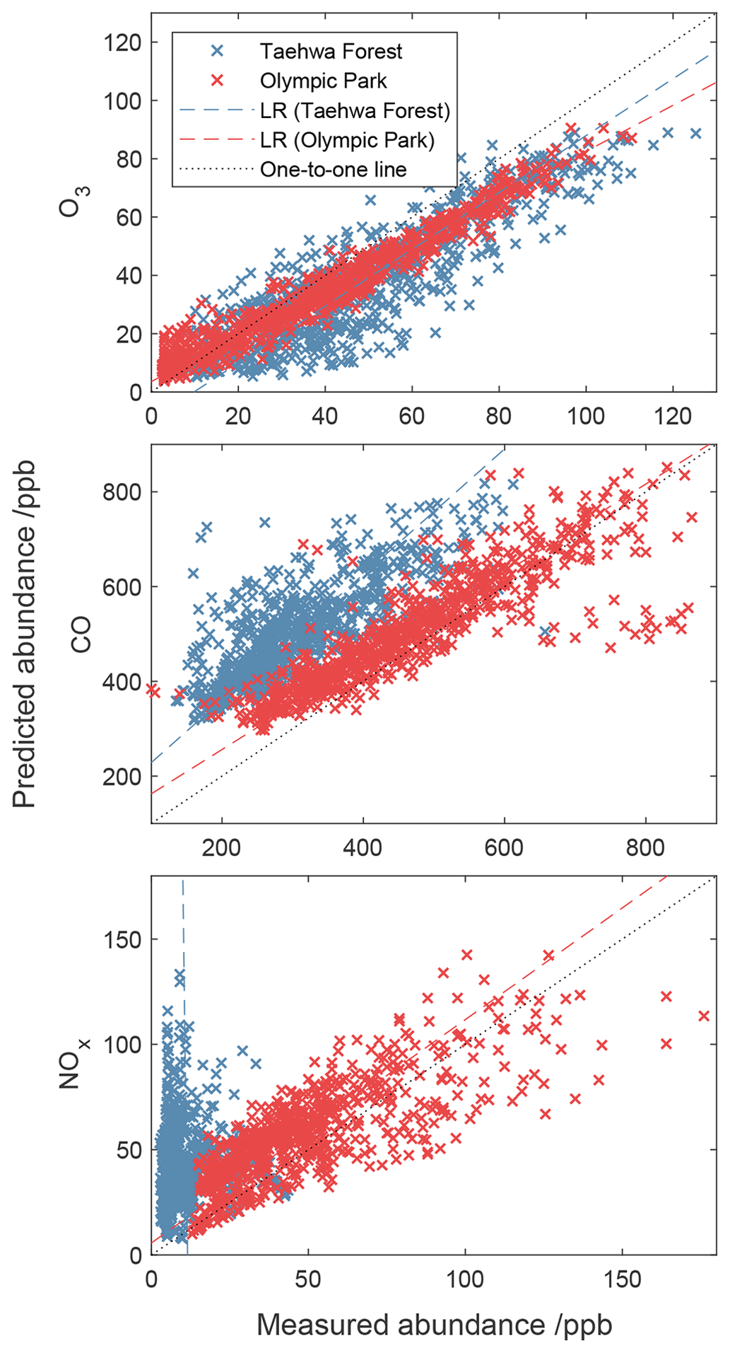
Figure 5 Predicted vs. measured abundances of the three key species at the Olympic Park (red) and Taehwa Forest (blue) research stations. Predicted abundances are computed as point interpolations as per Eq. (1). Dashed lines are linear regression (LR) models fitted by ordinary least squares.

Table 1 The generalized coefficients of determination $R_{E\mathrm{1}}^{\mathrm{2}}$, $R_{E\mathrm{2}}^{\mathrm{2}}$, and $R_{E\mathrm{3}}^{\mathrm{2}}$ (Eq. 5) for predictions vs. measurements at research stations (Olympic Park and Taehwa Forest) and along flight transects in the PBL. Each flight transect is a median of contiguous 10 s observations through a grid cell (see Fig. 1 for sampling distribution and Fig. 5 for scatter plots), and the predictions are gridded values interpolated linearly in time to match the aircraft time of flight and then averaged. E1, E2, and E3 are time series of prediction errors defined in Eq. (4). NO_x measurements at Taehwa Forest are taken from Kim et al. (2022).

As an isolated wilderness site, Taehwa Forest presents a unique problem for interpolating NO_x values based on NIER stations. The closest three NIER sites surround the forest station at a distance of around 10–15 km, and all are subject to NO_x roadside emissions; thus our interpolation maps these high-NO_x values into the relatively NO_x-depleted forest.

4.2 DC-8 comparison

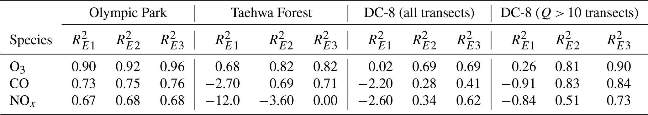
Figure 6 (top panel) shows that the gridded surface site predictions of the DC-8 O₃ observations are consistently lower than observed but remain strongly correlated. CO predictions (Fig. 6, middle panel) show a consistent bias of around +100 ppb but otherwise capture the variability in the aircraft CO measurements reasonably well. NO_x predictions (Fig. 6, bottom panel) show a consistent positive bias along with randomness in the low measured range (< 10 ppb). The gridded O₃ and CO predictions are highly accurate ($R_{E\mathrm{2}}^{\mathrm{2}}$ = 80 %) in grid cells with effective observation density (Q) exceeding 10, mainly sampled in the Seoul Metropolitan Area (Fig. 1, right-hand side). These findings show that with enough ground information, our gridded O₃ and CO datasets can predict upper PBL variability even in regions with intense small-scale emission heterogeneity. NO_x is exceptional, however, due to the rapid fall-off in abundance with altitude even within the PBL (Fig. A2 of Appendix A; see also Fig. 2 from Kim et al., 2021). We believe that O₃ titration in the Seoul Metropolitan Area leads to a slight underestimation in predicted variability, as shown by a 10 % increase in predictability using linear regression ($R_{E\mathrm{3}}^{\mathrm{2}}$ = 90 %, Table 1). We note however that the recurring flight patterns did not uniformly sample our grid domain and may have over- or undersampled some regions. Obtaining vertically averaged concentrations rather than surface values remains a challenge given the substantial near-surface gradients inferred from Figs. 6 and A2, and this suggests the need for vertically resolved chemical and dynamical modelling.

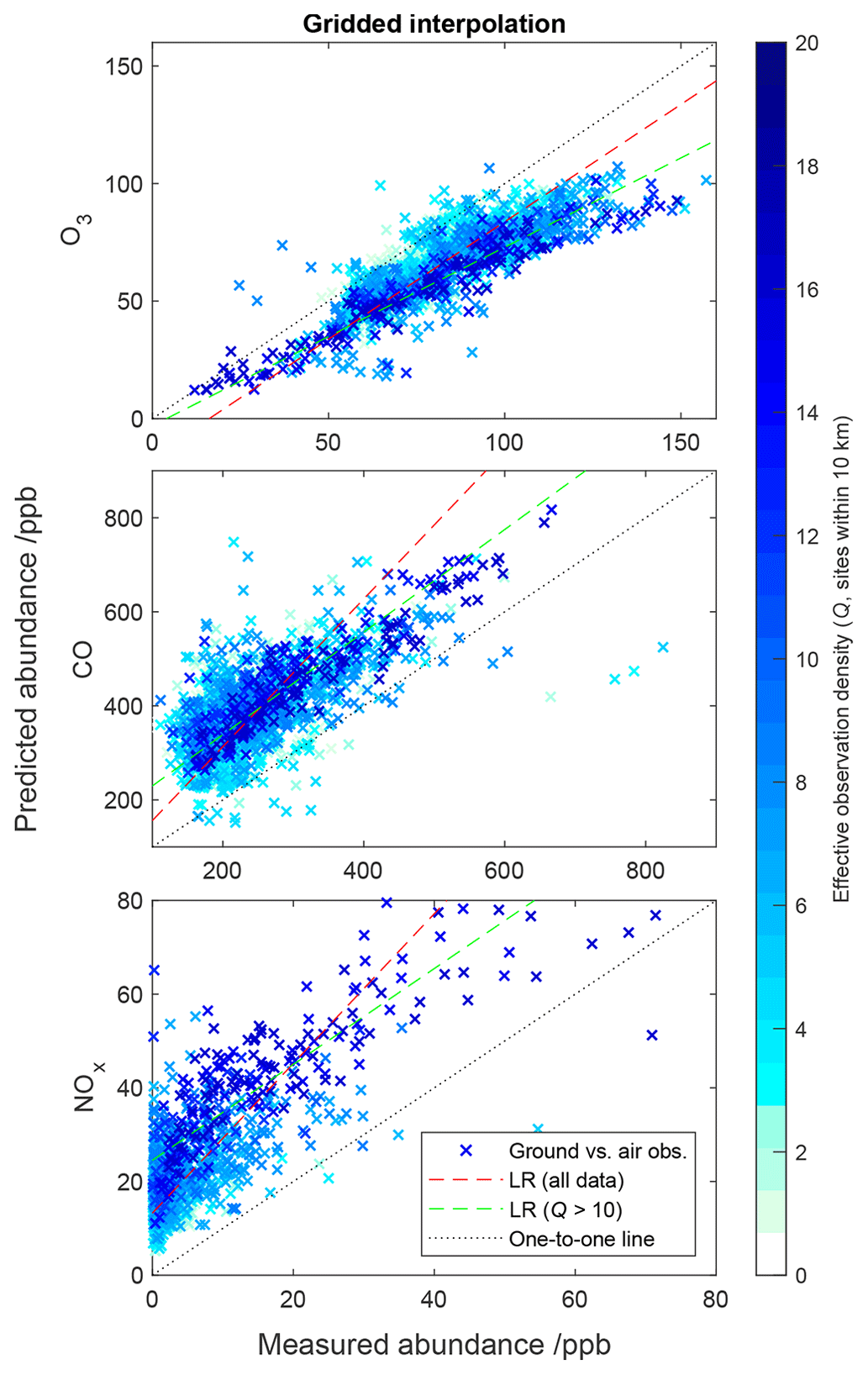
Figure 6 Comparison of 10 s DC-8 observations in the PBL and gridded (0.1° × 0.1°) hourly ground station data. Each data point represents the median of the contiguous aircraft transect through a grid cell (y axis) and the median of the gridded ground station data interpolated linearly in time to match the aircraft time of flight (x axis).

5 Conclusions

We create gridded (0.1° × 0.1°) observational datasets from NIER ground station measurements of air quality over South Korea. Unlike the arithmetic mean gridding technique, this method includes information from all nearby stations, including those outside the cell boundary, while mitigating sampling bias from site clustering. We identified significant mean absolute deviations between the IDW and arithmetic mean gridding techniques in, for example, the Seoul Metropolitan Area, where IDW proved most accurate, prompting caution with respect to the use of arithmetic mean gridding.

Our results suggest that the mean of and variability in ground-level O₃ were well captured over the whole of South Korea. For CO and NO_x, our LOOCV analysis revealed mean biases in certain NIER site predictions but otherwise good prediction accuracy in most densely observed urban regions after the biases were subtracted. The well-predicted regions include the Seoul Metropolitan Area, Busan, Changwon, Daegu, and Cheongju, whereas prediction accuracy was poorer in the conjoined coastal cities of Gwangyang, Yeosu, and Suncheon, as well as in Ulsan; predictability in these regions would benefit from denser sampling. The aircraft comparisons confirm that the variability in O₃ and CO in the PBL is well captured from the surface stations; however, NO_x vertical gradients in the PBL confound attempts to predict the aircraft NO_x measurements.

Inverse distance weighting is susceptible to errors from over- or undersampling of intense emission sources such as roadsides and industrial sectors. The characteristic concentrations of these regions may also be projected beyond the reach of the emission sources as seen in the high CO and NO_x biases at Taehwa Forest. These error sources are not unique to IDW. Nevertheless, improvements in NO_x predictability might be found with land-use regression and machine learning approaches as reviewed by Karroum et al. (2020), although these are outside the scope of the present paper. Such techniques can account for reactive NO_x decay away from sources, potentially mitigating errors from source sampling bias and over-projection. It would be interesting to compare the site predictability values vs. sampling density for these alternate techniques, particularly in regions that were undersampled according to LOOCV.

Appendix A

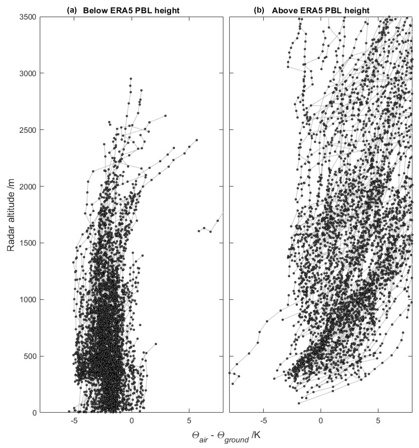
Figure A1 DC-8 10 s potential temperature (θ_air) measurements (dots) in a 0.5° radius of Taehwa Forest research station with gridded (0.25° × 0.25°) surface potential temperature (θ_ground) subtracted, taken below (a) and above (b) the ERA5 designated PBL height. Lines connecting dots indicate contiguous transects, and all data were taken during ascent or descent (aircraft vertical speed > 1 m s⁻¹). θ_ground was calculated using the ERA5 2 m temperature and surface pressure fields at native resolution (0.25° × 0.25°, hourly), interpolated in time to match the aircraft time of flight.

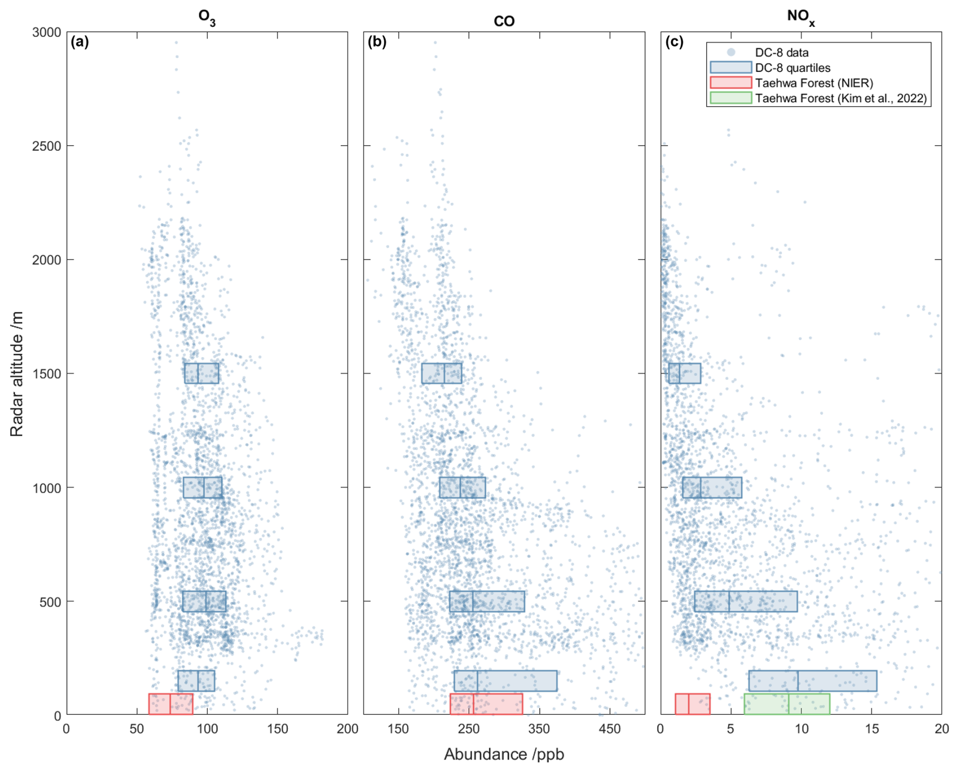
Figure A2 Vertical profiles of the DC-8-measured O₃ (a), CO (b), and NO_x (c) in the ERA5 PBL within a 0.5° radius of Taehwa Forest research station. All data are sampled between the hours of 12:00 and 17:00 LT, and quartiles are shown for aircraft data (blue) partitioned into altitude bins (0–250, 250–750, 750–1250, and 1250–1750 m) and for the available ground research station measurements at Taehwa Forest (red) supplemented by Kim et al. (2022) (green).

Appendix B

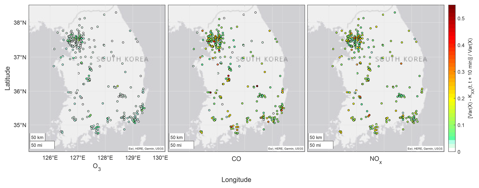
Figure B1 The sub-10 min temporal variability in the quality-controlled O₃ (left), CO (middle), and NO_x (right) site data at 5 min resolution. Sub-10 min variability for individual sites was calculated as the site autocovariance subject to a 10 min phase shift $\left(K_{XX}\right(t,t+\mathrm{10}\min \left)\right)$ subtracted from the total site variance (Var(X)), normalized by Var(X).

Appendix C

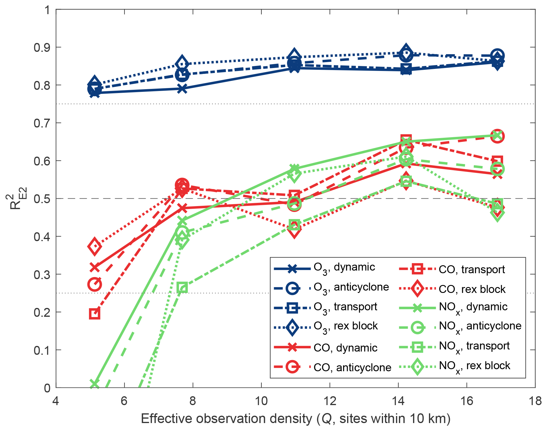
Figure C1 The median prediction accuracy ($R_{E\mathrm{2}}^{\mathrm{2}}$) of O₃ (blue), CO (red), and NO_x (green) within percentile bins (0 %–20 %, 20 %–40 %, 40 %–60 %, 60 %–80 %, and 80 %–100 %) during the meteorological phases (dynamic, anticyclone, transport, and Rex blocking) described by Peterson et al. (2019).

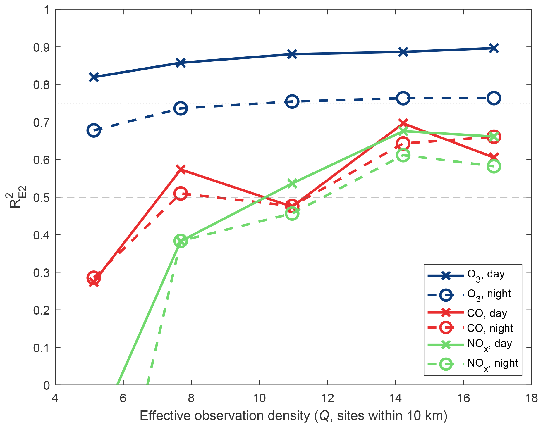
Figure C2 As in Fig. C1 but for daytime (07:00 to 20:00 LT inclusive) and nighttime (21:00 to 06:00 LT inclusive) data.