Mitigation of satellite OCO-2 CO₂ biases in the vicinity of clouds with 3D calculations using the Education and Research 3D Radiative Transfer Toolbox (EaR³T)

Accurate and continuous measurements of atmospheric carbon dioxide (CO₂) are essential for climate change research and monitoring of emission reduction efforts. NASA's Orbiting Carbon Observatory (OCO-2 and 3) satellites have been deployed to infer the column-averaged CO₂ dry-air mixing ratio (X${}_{{\mathrm{CO}}_{\mathrm{2}}}$) from passive spectroscopy, with a designed uncertainty of less than 1 ppm for the regional average. This accuracy is often not met in cloudy regions because clouds in the vicinity of a footprint introduce biases in the X${}_{{\mathrm{CO}}_{\mathrm{2}}}$ retrievals. These arise from limitations in the one-dimensional (1D) forward radiative transfer (RT) model, which does not capture the spectral radiance perturbations introduced by clouds adjacent to a clear footprint. Our paper introduces a three-dimensional (3D) RT pipeline to explicitly account for these effects in real-world satellite observations. This is done by ingesting collocated imagery and reanalysis products to calculate the cloud-induced perturbations at the footprint level. To make that computationally feasible, a simple approximation for their spectral dependence is used. The calculated perturbations are then used to reverse (undo) the cloud vicinity effects at the radiance level, at which point the standard 1D OCO-2 retrieval code can be applied without modifications. For two cases over land, we demonstrate that this approach indeed reduces the X${}_{{\mathrm{CO}}_{\mathrm{2}}}$ anomalies near clouds. We also characterize the dependence of the X${}_{{\mathrm{CO}}_{\mathrm{2}}}$ footprint-level bias on the distance from clouds and other key scene parameters, such as surface reflectance. Although this dependence may be specific to cloud type, aerosols, and other factors, we illustrate how it could be parameterized to bypass our physics-based 3D-RT pipeline for use in an operational framework. In the future, we intend to explore this possibility by applying our tool to a variety of scenes over land and ocean.

1 Introduction

Precise global carbon dioxide (CO₂) measurements are essential for a deeper understanding of surface CO₂ sources and sinks and their response to climate change, emissions reductions, and other mitigation strategies. The Greenhouse Gases Observing Satellites (GOSAT, GOSAT-2; Nakajima et al., 2010; Imasu et al., 2023) and the Orbiting Carbon Observatory (OCO-2, OCO-3; Crisp, 2015; Eldering et al., 2019), launched by the Japan Aerospace Exploration Agency (JAXA) and NASA, respectively, are currently in space to observe CO₂ and other greenhouse gases. They have been designed to precisely measure CO₂ column dry-air mixing ratios (X${}_{{\mathrm{CO}}_{\mathrm{2}}}$) through the analysis of reflected solar radiances in the oxygen A-band at 765 nm (O₂ A), as well as the weak and strong CO₂ bands near 1.61 µm (WCO₂) and 2.06 µm (SCO₂). High accuracy is imperative for remote sensing measurements of X${}_{{\mathrm{CO}}_{\mathrm{2}}}$ to effectively contribute to carbon flux (sources and sinks) studies. Miller et al. (2007) suggest that the regional uncertainty should be within 0.3 %–0.5 % (1 to 2 ppm) to meaningfully contribute to carbon flux estimates. Deng et al. (2016) and Crowell et al. (2018) highlight the importance of achieving high X${}_{{\mathrm{CO}}_{\mathrm{2}}}$ measurement accuracy for reliable CO₂ flux estimation. Deng et al. (2016) show that the assimilation of GOSAT X${}_{{\mathrm{CO}}_{\mathrm{2}}}$ data with a precision of approximately 0.5–1.0 ppm can significantly improve regional CO₂ flux estimates over land and ocean. Similarly, Crowell et al. (2018) emphasize that an X${}_{{\mathrm{CO}}_{\mathrm{2}}}$ precision of 0.5–1.0 ppm is essential for detecting regional flux perturbations, especially in cloud-prone and high-latitude regions where CO₂ fluxes are difficult to constrain accurately using ground-based sensors alone. Precision and accuracy in CO₂ remote sensing are contingent on factors including spectroscopy, calibration, aerosol scattering and absorption, and atmospheric water vapor (Nelson et al., 2022; Worden et al., 2017; Connor et al., 2016). The OCO missions employ an X${}_{{\mathrm{CO}}_{\mathrm{2}}}$ retrieval algorithm that integrates these elements along with observational conditions, such as solar zenith angle (SZA), viewing zenith angle, and geolocation (OCO-2 L2 ATBD, 2020), and uses a priori data such as CO₂ vertical profiles and surface reflectance to initialize spectral calculations via a computation-efficient one-dimensional (1D) radiative transfer (RT) model. The retrieval process iteratively refines the initial a priori estimates through optimal estimation methods (Rogers, 2000) until convergence between calculated and observed spectra is achieved.

Despite advancements in trace gas retrieval algorithms, the presence of clouds near satellite footprints remains a significant challenge. While retrievals typically exclude measurements over cloudy regions, photons scattered by nearby clouds can bias X${}_{{\mathrm{CO}}_{\mathrm{2}}}$ retrievals due to the neglect of photon transfer between atmospheric columns in the 1D-RT model. Recent studies (Massie et al., 2017, 2021, 2023; Kylling et al., 2022) have highlighted the presence of the three-dimensional (3D) cloud bias in trace gas retrievals, including OCO and TROPOspheric Monitoring Instrument (TROPOMI) nitrogen dioxide (NO₂) retrievals. The cloud-related bias is also evident when examining individual footprints. With clouds covering roughly 70 % of the globe (Wylie et al., 2005; King et al., 2013) and 40 % of the OCO-2 measurements being within 4 km of clouds (Massie et al., 2021), addressing cloud-induced bias is crucial for refining X${}_{{\mathrm{CO}}_{\mathrm{2}}}$ retrieval accuracy.

Schmidt et al. (2019) explain that lateral photon transport represents missing physics in the operational OCO algorithm, and any adjustments for differences between 1D-RT and 3D-RT could introduce additional inaccuracies in X${}_{{\mathrm{CO}}_{\mathrm{2}}}$ retrieval. Evaluating these differences requires a high-resolution 3D-RT model capable of simulating spectra across multiple wavelengths. Recent advancements have accelerated high-resolution 3D-RT simulations for multiwavelength applications. For instance, Partain et al. (2000) introduced an enhanced implementation of the equivalence theorem, which decouples scattering and absorption calculations, allowing for accurate spectral integration without repeated multiple-scattering computations for Monte Carlo models. Emde et al. (2011) developed the Absorption Lines Importance Sampling (ALIS) technique, which efficiently computes high-resolution polarized spectra by leveraging Monte Carlo photon tracing across multiple wavelengths simultaneously. Iwabuchi and Okamura (2017) also adopted a similar way of using the same photon paths for various wavelengths to accelerate multiwavelength 3D-RT simulation. Doicu et al. (2020) accelerated the spherical harmonics discrete ordinate method (SHDOM) 3D-RT model, which is different from Monte Carlo-based 3D radiative transfer models, by combining the correlated k-distribution method with dimensionality reduction techniques, such as principal component analysis.

While these acceleration methods have the potential to improve the accuracy of trace gas retrievals by taking into account missing physics (horizontal photon transport), current operational retrievals still do not use true 3D-RT in trace gas retrieval processes. Here, we adopt the approach introduced by Schmidt et al. (2019) as a practical method to approximate the 1D-RT and 3D-RT differences in spectral radiance observations, building on the concept of 3D-RT radiance perturbations, defined as the spectral percentage difference between 3D and 1D radiance simulations. The simulations in this study are performed using a modified version of the Education and Research 3D Radiative Transfer Toolbox (EaR³T; Chen et al., 2023), tailored specifically for OCO (EaR³T-OCO). The 3D perturbations proved to be a linear function of the radiance (or reflectance) itself across the relevant dynamic range of reflectance, which allows its representation by a simple slope and intercept for each of the three OCO-2 bands, with further details provided in Sect. 2. We also introduce a “bypass” parameterization that relates slopes and intercepts to factors such as cloud distance and scene reflectance, enabling the quantification of 3D cloud effects under varying conditions.

Although the reflectance-dependent physical mechanisms of the X${}_{{\mathrm{CO}}_{\mathrm{2}}}$ 3D cloud retrieval bias are now largely understood, strategies for applying these insights to bias correction have thus far been done empirically or statistically. For example, Massie et al. (2023) proposed an empirical lookup table to correct 3D cloud biases based on a 3D metric, and Mauceri et al. (2023) used machine learning techniques combined with Total Carbon Column Observing Network (TCCON) observations. While both approaches are operationally applicable, they rely on statistical corrections rather than the actual physical radiance difference in the 3D cloud effect across the entire spectrum. In contrast, we present a new physics-based mitigation framework that directly applies the linear representation of the 3D cloud effect to real OCO-2 observations. This approach aims to remove the 3D perturbation at the radiance level before reapplying the operational 1D retrieval, thereby improving the accuracy of the retrieved X${}_{{\mathrm{CO}}_{\mathrm{2}}}$.

The remainder of this paper is organized as follows: Sect. 2 provides background on the linear 3D perturbation concept. Section 3 details data used in this study and EaR³T-OCO simulation. Section 4 (and Appendix B) outlines our methodology for deriving slope and intercept parameters at a limited set of wavelengths and for using them to mitigate X${}_{{\mathrm{CO}}_{\mathrm{2}}}$ biases. Section 5 shows how these parameters are used to correct the observed radiance spectra and, by extension, the retrieved mitigated X${}_{{\mathrm{CO}}_{\mathrm{2}}}$. Finally, Sect. 6 provides conclusions, and Sect. 7 discusses future work. Appendix C explains the functionality of EaR³T-OCO in detail.

2 Background information

This study builds on Schmidt et al. (2019), which found a linear relationship between radiance perturbations and reflectance due to 3D-RT effects. They define the 3D-RT radiance perturbation as the percent difference between the radiances calculated by 3D and 1D radiative transfer models, as formulated in Eq. (1).

$$\begin{array}{}\text{(1)}& {\mathrm{Perturbation}}_{\mathit{\lambda }}={\displaystyle \frac{I_{\mathit{\lambda }}^{\mathrm{3}\mathrm{D}}-I_{\mathit{\lambda }}^{\mathrm{IPA}}}{I_{\mathit{\lambda }}^{\mathrm{IPA}}}}={\displaystyle \frac{I_{\mathit{\lambda }}^{\mathrm{3}\mathrm{D}}}{I_{\mathit{\lambda }}^{\mathrm{IPA}}}},\mathrm{1}\end{array}$$

The magnitude of this perturbation is not uniform across the observed wavelength spectrum but depends on the reflectance (R_λ), defined as follows:

$$\begin{array}{}\text{(2)}& R_{\mathit{\lambda }}={\displaystyle \frac{I_{\mathit{\lambda }}\times \mathit{\pi }}{S_{{\mathrm{0}}_{\mathit{\lambda }}}^{\mathrm{TOA}}\times \cos {\mathit{\theta }}_{\mathrm{s}}}},\end{array}$$

where $S_{{\mathrm{0}}_{\mathit{\lambda }}}^{\mathrm{TOA}}$ in the denominator denotes the solar irradiance at the top of the atmosphere (TOA) for a given wavelength λ, and θ_s is the solar zenith angle.

Within the dynamic range of interest for reflectance, the dependence of the perturbation on the reflectance is linear. This is illustrated in Fig. 1, which shows simulated observations in the O₂ A-band (Schmidt et al., 2019). For small reflectance, the scatter increases due to a limited number of photons in the calculations (Appendix B4). A line is fitted to the data to represent the first-order dependence of the 3D-RT perturbation on the reflectance. This can be done with either all wavelengths (grey dots) or a subset (red), which is strategically chosen to encompass the full reflectance range.

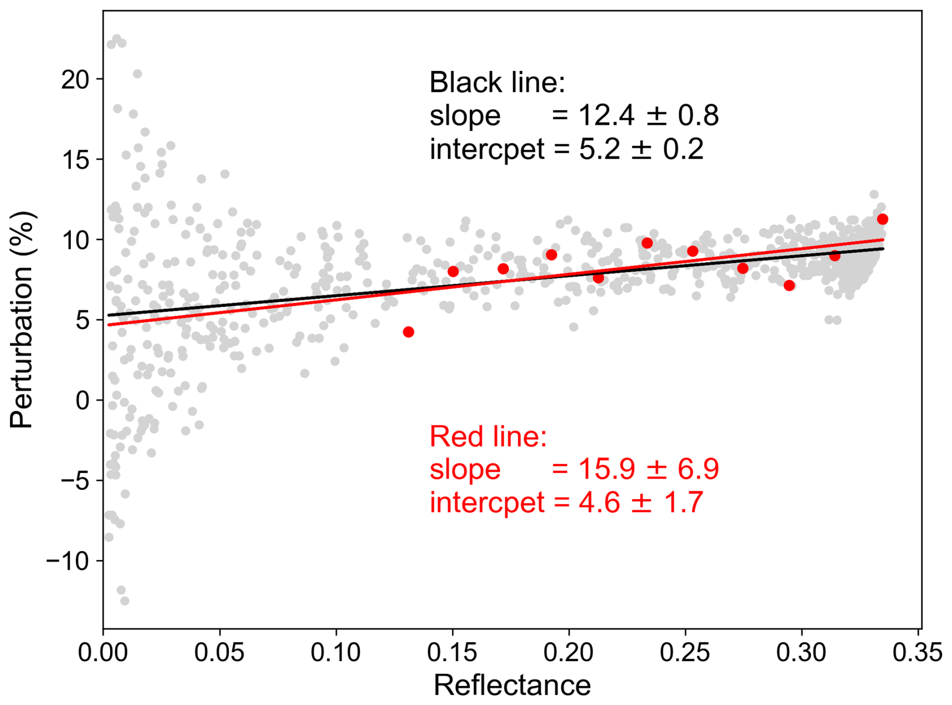
Figure 1 Example of the linear relationship between perturbation and reflectance. The grey dots represent the complete wavelength range, while the red dots indicate the subset selected for the O₂ A-band simulation. The black and red lines represent the linear fits of the grey and red dots, respectively.

The slope and intercept parameters, s_xy and i_xy, are obtained through weighted linear regression as shown in Eq. (3), where the weights are the inverse of the perturbation uncertainty (computational noise; see Appendix B4). The slope and intercept indicate distinct physical phenomena: a nonzero slope corresponds to wavelength-dependent variations and differences in 1D and 3D radiances, photon path lengths, and absorption. Multiple scattering in 3D-RT increases the photon path lengths and enhances absorption across different wavelengths, leading to nonzero perturbations, as expressed by Eq. (1) (percentage differences between 1D and 3D radiances). This effect is more pronounced at wavelengths with higher absorption, which experience greater attenuation compared to those with weaker absorption for the same photon path length. As a result, the perturbations vary depending on the reflectance and absorption depth, a phenomenon referred to as spectral distortion in our study. The intercept is related to the often-reported increase in reflectance near clouds or decrease in shadows, whereas the slope accounts for spectroscopic effects for a small spectral range, where the scattering effect can be considered spectral-independent.

$$\begin{array}{}\text{(3)}& {\mathrm{Perturbation}}_{\mathit{\lambda }}=i_{xy}+s_{xy}\times R_{\mathit{\lambda }}^{\mathrm{3}\mathrm{D}}\end{array}$$

3 Data

3.1 OCO-2 data

Version 10r OCO-2 data, hosted by NASA's Goddard Earth Science Data and Information Services Center (GES DISC) archive (https://oco2.gesdisc.eosdis.nasa.gov/data/OCO2_DATA, last access: 25 October 2024), are used in this research. The Level 1B calibrated and geolocated science radiance spectra (L1bScND) are specified in all three OCO-2 bands, facilitating simulation comparison and retrieval adjustment. Additionally, solar zenith and azimuth angles, as well as viewing zenith and azimuth angles from this product, serve as inputs for the simulation. The standard Level 2 geolocated X${}_{{\mathrm{CO}}_{\mathrm{2}}}$ retrieval results (L2StdND) provide the retrieved CO₂ dry-air mixing ratio and surface reflectance information for the three bands. Note that the X${}_{{\mathrm{CO}}_{\mathrm{2}}}$ in the L2StdND files is raw X${}_{{\mathrm{CO}}_{\mathrm{2}}}$ before the bias correction provided by the algorithm team. We also employed Level 2 meteorological parameters interpolated from the global assimilation model for each sounding (L2MetND) and Level 2 CO₂ prior profile based on the CO₂ monthly flask record, global meteorology, and age of air (L2CO2Prior) to construct the atmosphere for the simulation (refer to Appendix B1).

3.2 MODIS Aqua data

The MODIS Aqua satellite, launched in May 2002, is part of NASA's A-Train constellation but exited the formation due to fuel issues. As MODIS Aqua shared the same orbit as OCO-2 and arrived at the same scene approximately 6 min after OCO-2, the collocated information from MODIS Aqua offers valuable insights into the meteorological and surface conditions of the OCO-2 footprints and the spatial distances of clouds to the footprints. Several products derived from MODIS Aqua observations are used in this study, including MODIS Level 1B radiance products at the 0.25, 0.5, and 1 km scales (channels 1 to 7, MYD02QKM, MYD02HKM, and MYD021KM; MODIS Characterization Support Team (MCST), 2017a–c), the geolocation product (MYD03, MODIS Characterization Support Team (MCST), 2017d), the Level 2 cloud product (MYD06, Platnick et al., 2015), the Level 2 aerosol product (MYD04_L2, Levy and Hsu, 2015), and the surface reflectance product (MCD43A3, Schaaf and Wang, 2021) from data collection 6.1. These various products contribute to a comprehensive understanding of the atmospheric and surface conditions relevant to the OCO-2 measurements, thereby enhancing the accuracy and reliability of our analysis.

4 Methods

4.1 Case description

In order to investigate the X${}_{{\mathrm{CO}}_{\mathrm{2}}}$ retrieval biases resulting from cloud scattering, we have selected a case that features high X${}_{{\mathrm{CO}}_{\mathrm{2}}}$ anomalies in close proximity to clouds, as shown in Fig. 2. The chosen case is located in central Asia, spanning 33.85° N, 55.15° E to 34.30° N, 55.45° E. The study focuses on the conditions observed on 18 October 2018, with stronger reflectance for all three OCO-2 bands. The surface level based on the MODIS MYD03 file is shown in Fig. A1, with the OCO-2 Met file specifying an average altitude near 790 m. The average solar zenith angle and observation zenith angle for OCO-2 footprints are 48.5 and 0.31°, and the mean surface albedos for the O₂ A, WCO₂, and SCO₂ bands are 0.288, 0.375, and 0.370, respectively. The average aerosol optical depth (AOD) at 550 nm from the MODIS MYD04 file is 0.179 over the domain. Figure A1 specifies the surface altitude level from the MODIS MYD03 data file, in addition to the atmosphere profile for this case, derived by the method described in Appendix B1.

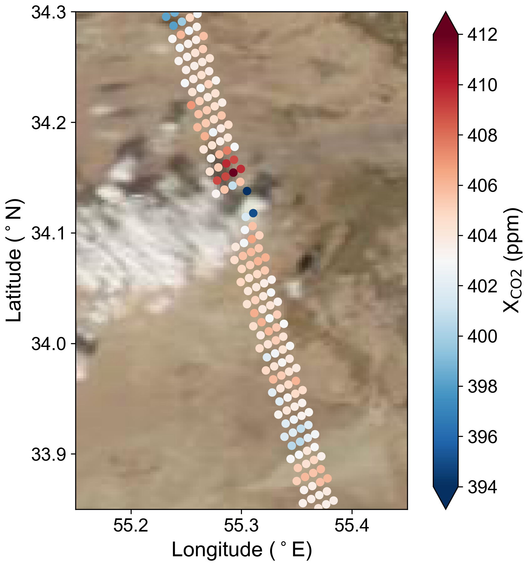
Figure 2 Satellite true-color imagery of MODIS Aqua from NASA Worldview on 18 October 2018, with OCO-2 retrieved X${}_{{\mathrm{CO}}_{\mathrm{2}}}$ overlaid.

4.2 Overview of radiative transfer model simulation

The Education and Research 3D Radiative Transfer Toolbox v0.1.1 (Chen et al., 2023) for OCO (EaR³T-OCO) was adapted to simulate 1D and 3D radiances for OCO-2 observations. The RT model simulates the photon–environment interactions based on the physical mechanisms that are understood, such as absorption, scattering, and reflection. Since this research aims to investigate the differences between 1D and 3D radiances, referred to as 3D radiative perturbations, both 1D and 3D RT calculations are utilized. These perturbations, expressed as linear functions of reflectance, are parameterized with slope and intercept values for each spectral band. The atmospheric environment used for the RT simulation also impacts the results. Detailed descriptions of the atmospheric structure, vertical layering, and the computation of number densities for absorption coefficients are provided in Appendix B.

4.3 Perturbations, reflectance, slopes, and intercept derivation

Building on the foundational concepts of perturbation and reflectance introduced in Sect. 2 (refer to Eqs. 1–2), we run the EaR³T-OCO simulator in 1D and 3D mode to calculate $I_{\mathit{\lambda }}^{\mathrm{IPA}}$ and $I_{\mathit{\lambda }}^{\mathrm{3}\mathrm{D}}$. From these simulated radiances, we obtain the reflectances and perturbations. These are used to derive the slope and intercept parameters for quantifying the 3D effect. We apply a weighted linear regression (see Eq. 3) to ensure that more accurate data exert a greater influence on the parameter estimation. This approach yields not only the slope and intercept values but also their respective uncertainties, providing a comprehensive picture of the 3D effect's variability and reliability. The slope and intercept parameters obtained are used to quantify the magnitude of the 3D effect, a detailed discussion of which is presented in Sect. 5.2 to 5.5. Additionally, the parameters play a crucial role in the offline mitigation strategies explored in Sect. 5.6.

4.4 OCO retrieval algorithm and spectra mitigation

The retrieval algorithm plays a vital role in determining X${}_{{\mathrm{CO}}_{\mathrm{2}}}$ based on the radiances of the three bands. Notably, the retrieval algorithm accounts for various processes, and post-retrieval processing calculates linear bias corrections (O'Dell et al., 2018). Different retrieval versions may yield diverse outcomes even with identical inputs. In this study, we utilize the OCO retrieval algorithm version B10.04 to compare with version 10r X${}_{{\mathrm{CO}}_{\mathrm{2}}}$. The retrieval code is publicly available on NASA's GitHub repository (https://github.com/nasa/RtRetrievalFramework, last access: 24 January 2023).

Given that the 1D-RT model does not account for additional scattered photons, the mitigation strategy proposed in this study involves modifying the observed spectra to eliminate radiance changes induced by the 3D effect. This adjustment process is referred to as “radiance adjustment” and is derived from Eqs. (1) to (3). Upon deriving the 3D parameters in Sect. 4.3, we calculate the adjusted OCO-2 spectra $\left(I_{\mathit{\lambda }}^{\mathrm{IPA}\left(\mathrm{adjusted}\right)}\right)$ using Eq. (4) with the observed radiance spectra $\left(I_{\mathit{\lambda }}^{\mathrm{3}\mathrm{D}\left(\mathrm{obs}\right)}\right)$ and corresponding reflectance $\left(R_{\mathit{\lambda }}^{\mathrm{obs}}\right)$, slope (s_xy), and intercept (i_xy). Assuming the absence of 3D effects in the adjusted 1D radiance, we can employ the B10.04 retrieval algorithm to the adjusted spectra $\left(I_{\mathit{\lambda }}^{\mathrm{IPA}\left(\mathrm{adjusted}\right)}\right)$ to obtain mitigated X${}_{{\mathrm{CO}}_{\mathrm{2}}}$.

$$\begin{array}{}\text{(4)}& I_{\mathit{\lambda }}^{\mathrm{IPA}\left(\mathrm{adjusted}\right)}(x,y)={\displaystyle \frac{I_{\mathit{\lambda }}^{\mathrm{3}\mathrm{D}\left(\mathrm{obs}\right)}(x,y)}{(i_{xy}+s_{xy}\times R_{\mathit{\lambda }}^{\mathrm{obs}}+\mathrm{1})}}\end{array}$$

5 Results

5.1 3D-RT simulation radiance closure

In order to derive the slope (s) and intercept (i) parameters that accurately represent the 3D cloud effect in the OCO-2 observations, it is crucial to perform realistic radiance simulations near the satellite's footprint. Chen et al. (2023) show that the extent of radiance closure (the percent difference in the forward radiance model and observed radiances) can indicate the correctness of the retrieved cloud properties. Figure 3a–b present the 3D-RT simulation and MODIS observation of 650 nm using the cloud optical thickness (COT), cloud effective radius (CER), and cloud top height (CTH) shown in Fig. A2. The heat map in Fig. 3c shows good agreement between the simulation and observation, with an R² of 0.69 and a slope of 0.71. We then used the same CTH, CER, and COT settings to model the wavelengths in the O₂ A, WCO₂, and SCO₂ bands.

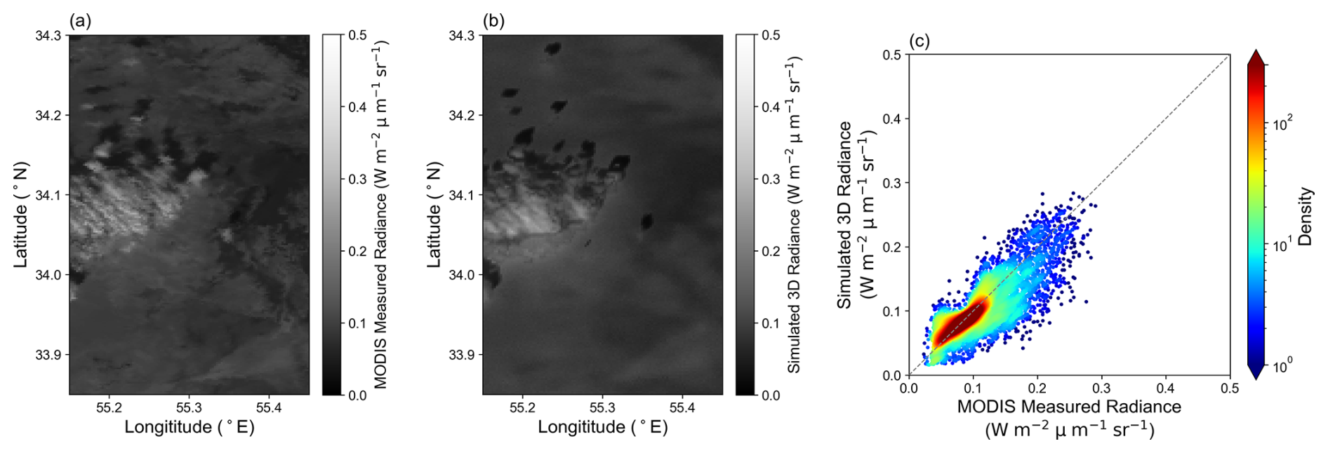
Figure 3 MODIS observation at 650 nm from MODIS MYD02QKM data (a) and 3D radiance simulation at 650 nm by EaR³T (b). A scatterplot comparison between (a) and (b) is depicted in (c).

Multiple reflectances or wavelengths are needed to derive s and i for the linear expression of the perturbations and reflectances of three bands. To balance computational demands with accuracy, we selected 11 wavelengths evenly distributed over the high 60 % transmittance based on sorted clear-sky transmittance for further RT simulation (depicted in Fig. 4 as an example, the transmittance of full spectra is presented in Fig. A3). The transmittance is calculated based on the atmosphere profiles of pressure, temperature, gas optical depth, aerosol optical properties, and cloud optical properties. This reduction in simulated wavelengths is feasible due to the linear relationship between perturbations and reflectance. Employing a reduced number of wavelengths uniformly distributed across the reflectance space effectively minimizes computational demands while still permitting the derivation of s and i for the linear relationships within each band. Note that the number of wavelengths (11) utilized for determining the 3D parameters is adaptable. Employing additional wavelengths could decrease the uncertainty in the derived s and i, albeit at the expense of increased computation time.

Since the radiance simulation is cyclic at the edges, leaking radiance from one edge to the other could introduce unrealistic artifacts from RT simulations. We extended the margin by 0.15° on each side but excluded the additional margins during the analysis. Figure A4 illustrates the simulation and the analysis domains, with cloud distribution and cloud distance serving as the background.

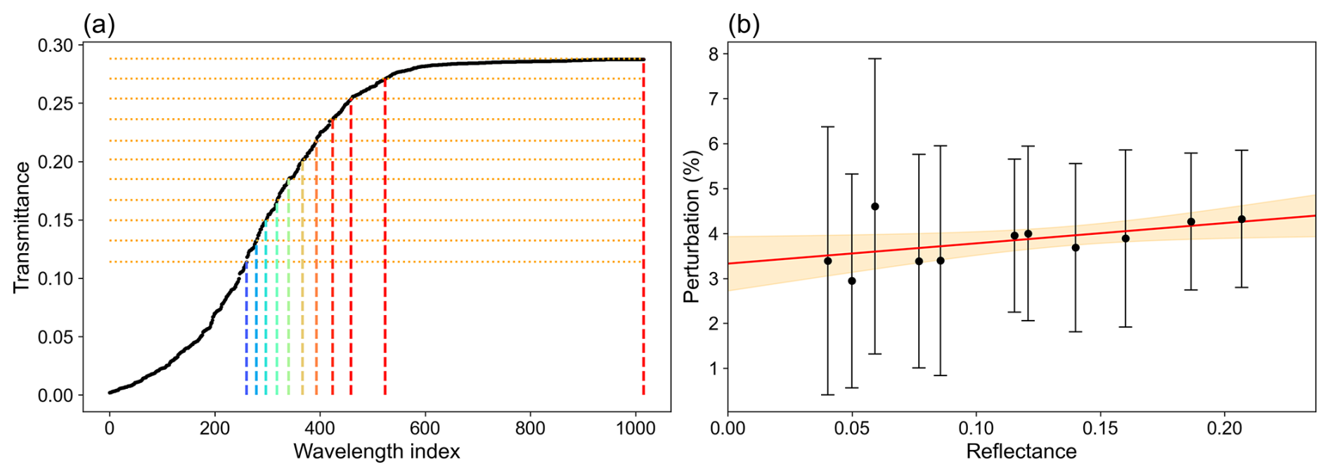
Figure 4 (a) Sorted clear-sky transmittance as per Appendix B2; the wavelength index presents the lowest to highest transmittance. (b) Illustration of the selected wavelength distribution in reflectance space versus the Eq. (3) perturbation for 34.08° N, 55.31° E.

5.2 3D cloud effect parameter analysis

We employed simulated radiance data across three distinct bands to quantify the 3D cloud effect perturbation: s and i. With the horizontal grid cell size around 0.25 km, we derived an approximate mean radiance for a 1 km² area by calculating the average radiance of the 5 × 5 nearest grid points, thereby approximating the OCO-2 footprint. We excluded the data if the 25 nearest grid points contained cloud pixels used in the RT simulation. The distribution of s and i for the O₂ A-band ($s_{{\mathrm{O}}_{\mathrm{2}}\text{ A}}$, $i_{{\mathrm{O}}_{\mathrm{2}}\text{ A}}$) is illustrated in Fig. 5, with the cloud positions denoted by red dots.

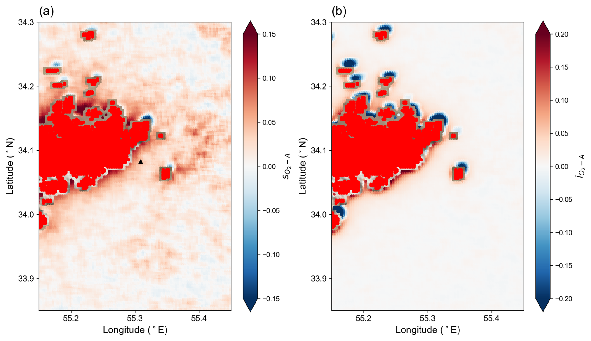
Figure 5 Distribution of (a) s and (b) i of the O₂ A-band. Red dots denote the cloud pixels employed in the RT simulation.

The analysis shows that the magnitudes of the 3D cloud effect parameters diminish (s and i get close to 0) as the grid point distance from the cloud increases. This decrease in magnitude corresponds to the smaller 3D cloud effect when the cloud is not in close proximity. Additionally, we divided the clear-sky area into two distinct categories: bright and shadow areas. The bright area represents grid points that receive more scattered photons, whereas the shadow area encompasses grid points within the cloud shadow region. Separating these categories is necessary due to the negative and positive intercepts associated with the shadow and bright areas. Notably, both categories exhibit positive s for the three different bands, exhibiting characteristics consistent with those described by Schmidt et al. (2019). Although it is instructive to discuss both cloud brightening and cloud shadowing effects, Massie et al. (2023) determined that there are relatively few cloud shadow retrievals in the OCO-2 Lite files since many observations impacted by shadowing are screened by the OCO-2 pre-retrieval cloud screening algorithms. Hereafter, bright-area analyses are the primary focus of our study.

Upon plotting s and i as a function of various definitions of the distance of a given pixel to the surrounding clouds, we identified an exponential decay relationship between the 3D cloud effect parameters and the effective horizontal cloud distance (D_e, Fig. 6), which is defined as the average distance of the pixel to the surrounding cloudy pixels weighted by the inverse square distance to the cloudy pixel (Eq. 5):

$$\begin{array}{}\text{(5)}& D_{\mathrm{e}}={\displaystyle \frac{{\sum }_{i\in \mathit{\left\{}\mathrm{surrounding}\mathrm{clouds}\right\}}{w}_i{D}_i}{{\sum }_{i\in \mathit{\left\{}\mathrm{surrounding}\mathrm{clouds}\right\}},w_i}}\end{array}$$

where D_i is the distance of a given pixel to a pixel location of a surrounding cloud, and $w_i=D_i^{-\mathrm{2}}$ is the weight. The exponential drop-off shown in Fig. 6 aligns with the result shown in Fig. 6 of Massie et al. (2021), although they used the nearest cloud distance.

The effective cloud distance (D_e) helps minimize the effect of a tiny isolated cloud versus multiple scattered clouds, as displayed in Fig. A4. This exponential decay relationship can be attributed to atmospheric attenuation proportional to their current values. Subsequently, we fitted these parameters and D_e using Eqs. (6)–(7):

$$\begin{array}{}\text{(6)}& {\displaystyle }\mathit{s}=a_s\times \exp \left(-{\displaystyle \frac{D_{\mathrm{e}}}{d_s}}\right)\text{(7)}& {\displaystyle }\mathit{i}=a_i\times \exp \left(-{\displaystyle \frac{D_{\mathrm{e}}}{d_i}}\right),\end{array}$$

where amplitude (a_s, a_i) and e-folding distance (d_s, d_i) are the fitting parameters (separate sets for s and i, the slope (s) and intercept (i) parameters that represent the 3D cloud effect). The data are partitioned into multiple columns, employing a bin size of 0.05 reflectance, and we utilize the median of each bin for the fitting procedure. However, we observed that the median s and i values did not approach zero as the cloud distance increased, possibly due to an inadequate number of grid points at larger cloud distances. To rectify this issue, we optimized the fitting coefficients by iteratively increasing the number of points employed in the fitting process until the maximum R² value was attained.

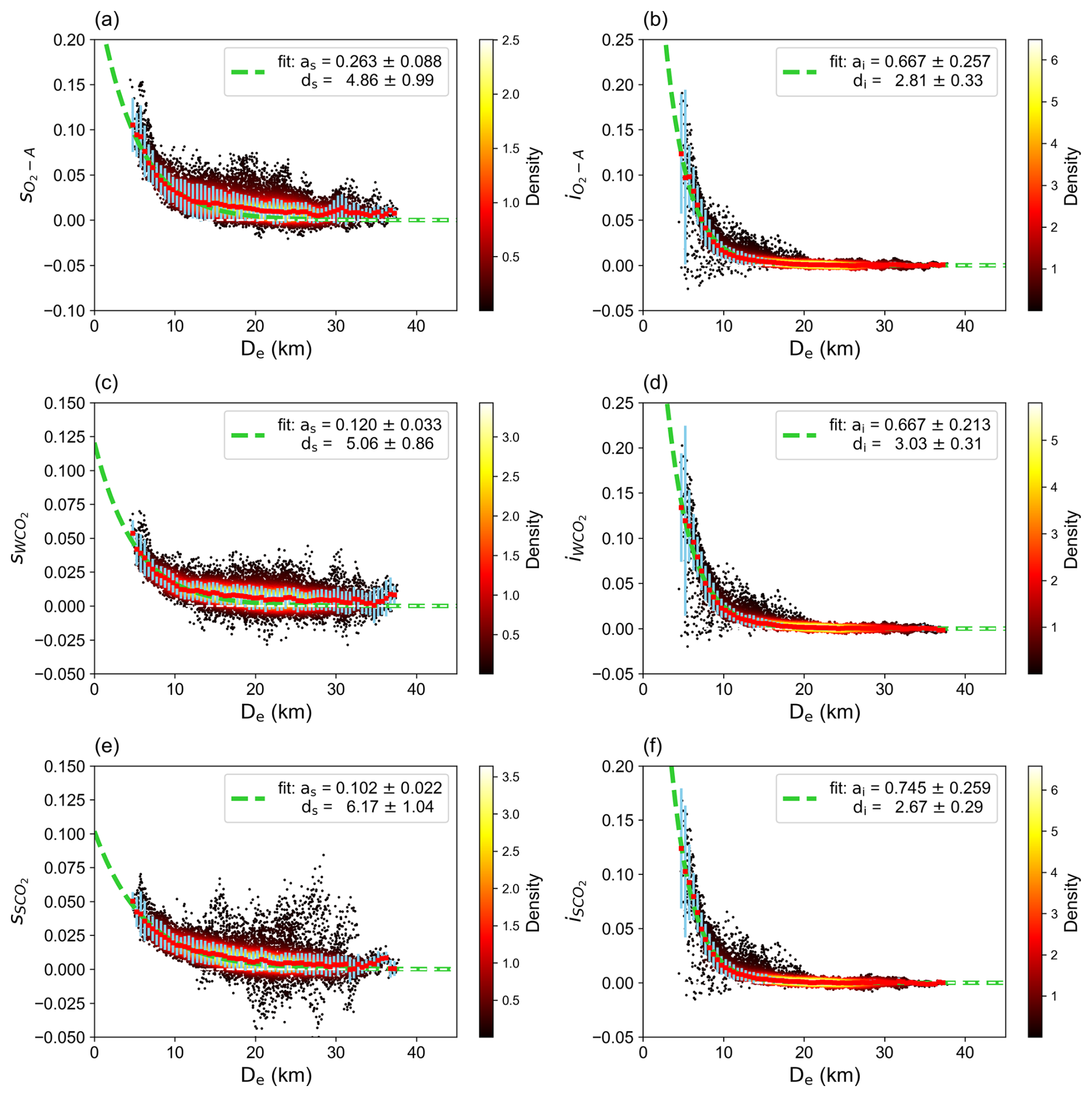
Figure 6 Exponential fitting (dashed green lines) of three bands in the bright area. The black dots present data from each pixel, while the background shading indicates the density of the black dots' distribution. The red points denote the median of each bin, and the blue error bars indicate the first and third quantiles for each bin.

The intercept parameter relates to what is traditionally known as the 3D-RT effect in spectrometry for a wavelength range with minimal gas absorption, whereas the slope is its spectroscopic equivalent, representing spectral distortion due to strongly varying gas absorption cross-sections over a wavelength range. Even slight changes in absorption may result in substantial changes in the retrieved trace gas concentration. The disparity in d_s for each band is not statistically significant, suggesting a similarity in the photon path histories across the different spectral bands.

The initial method, denoted the baseline method, applies Eq. (4) on an observation-pixel-by-pixel basis and uses only about 1 % of the available wavelengths in the three OCO-2 spectra. This method significantly reduces computation time for 3D-RT calculations for a given cloud scene. Next, using the exponential relationships in Eqs. (6)–(7), the 3D effect can be quantified by determining 12 3D-effect parameters: two amplitudes and two e-folding distances (a_s, d_s and a_i, d_i) for each band. These parameters can be applied to the full scene. Once the effective distance D_e is known for a pixel, the adjusted radiance $I_{\mathit{\lambda }}^{\mathrm{IPA}\left(\mathrm{adjusted}\right)}$ can be readily determined without further 3D-RT simulations (see Sect. 5.6 for examples). An ensemble of 12 3D-effect parameters can be calculated for various cloud spatial distributions, cloud properties, and associated aerosol optical depths. As discussed below in Sect. 5.5, the 12 3D-effect parameters can be further parameterized in terms of surface albedo and the cosine of SZA. This parametric approach will be denoted the bypass method, allowing for the evaluation of the 3D cloud effect and potentially eliminating the need for 3D-RT simulations altogether.

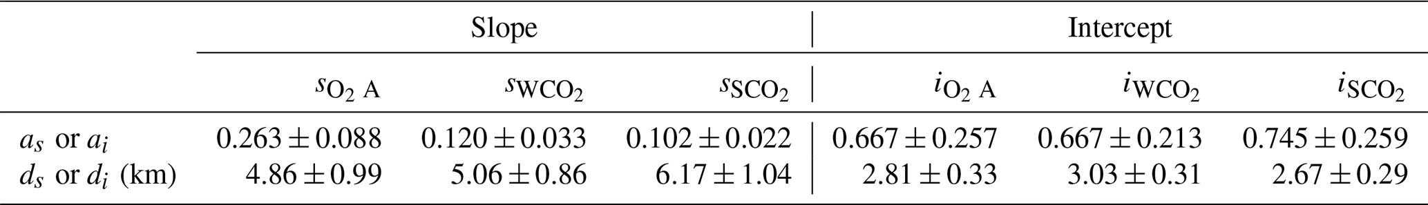
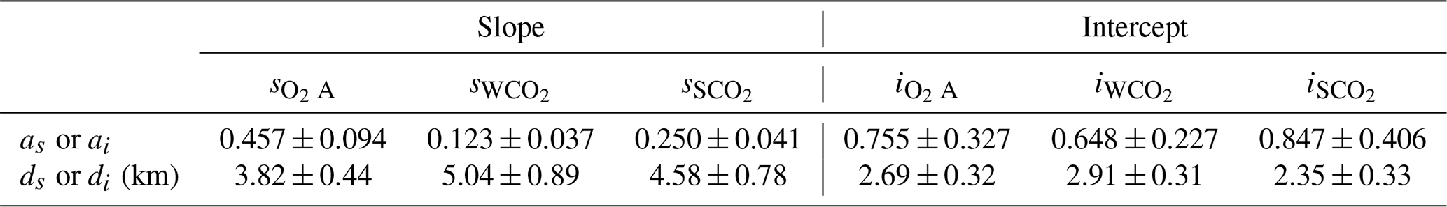
Table 1 Amplitude and e-folding distances for s and i fittings in the O₂ A, WCO₂, and SCO₂ bands for the simulation shown in Fig. 5. Errors represent fitting uncertainty only and may be underestimated.

5.3 Impact of aerosol

Upon establishing the relationship between the 3D cloud effect parameters and the cloud distance, we proceeded to analyze the impact of aerosols on this phenomenon since aerosols play an important role in shortwave radiation. In the presence of aerosols, photons near clouds experience increased extinction (scattering or absorption depending on aerosol radiative properties), making them travel shorter horizontal distances. Consequently, the e-folding distance is expected to be smaller when higher aerosol loading occurs. To maintain consistency with the previous section, we kept several variables constant, including COT, CER, CTH, cloud position, and atmospheric conditions. However, we introduced a homogeneous aerosol layer into the scenario to investigate its effect on the fitting amplitude and e-folding distance, as detailed in Sect. 5.2. The aerosol optical depth (AOD) data were obtained from the MODIS MYD04 data file using the aerosol optical depth and Ångström exponent at 550 nm. The top height of the aerosol layer was determined by the prevailing cloud top heights below 4 km, and we assumed uniform AOD values for layers beneath this top height. Aerosol optical depths in the O₂ A, WCO₂, and SCO₂ bands are 0.098, 0.038, and 0.024, respectively.

In the simulation incorporating aerosols, the analysis was conducted utilizing the methodology discussed in Sect. 5.2. Analogous correlations were identified between the 3D cloud parameters and D_e, as shown in Fig. 7 and Table 2. Notably, the presence of an aerosol layer exhibited a pronounced impact on the O₂ A and SCO₂ bands. This observation aligns with the absorption strength of each spectral band. Consequently, d_s associated with the O₂ A and SCO₂ bands witness a reduction while a_s of those two bands increases. This suggests that, in the presence of aerosols, the spectral distortion processes within the strong absorption bands are predominantly localized in proximity to the cloud. These findings underscore the pronounced influence of aerosols on the spectral distortion of bands with strong absorptivity.

Note that our simulation relied on the assumption of uniform aerosol distribution within the boundary layer, derived from the mean AOD obtained from the MODIS product. However, this assumption may not always hold true in real-world scenarios. We show that the presence of aerosols can lead to alterations in both the s and i of the O₂ A and SCO₂ bands, potentially increasing the uncertainty associated with the derivation of 3D-effect parameters.

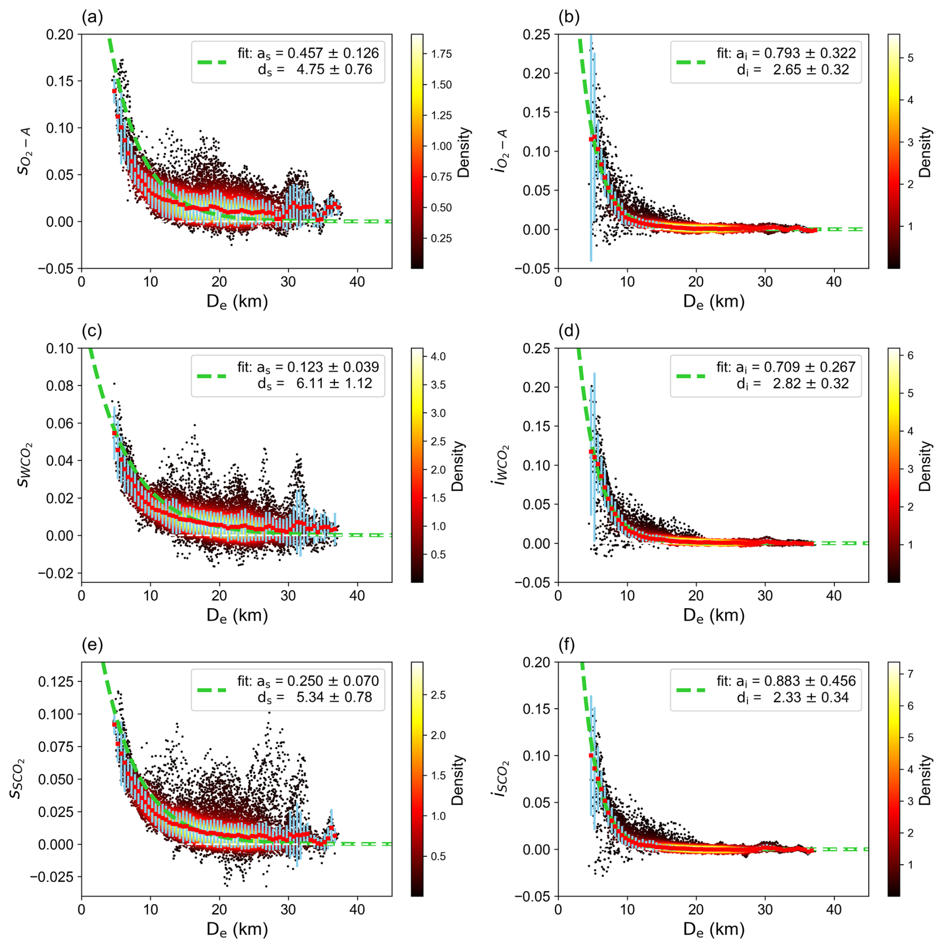
Figure 7 Exponential fitting (dashed green lines) of the three OCO-2 bands in the bright area of the simulation with a homogeneous aerosol layer. The black dots present data from each pixel, while the background shading indicates the black dots' distribution density. The red points denote the median of each bin, and the blue error bars indicate the first and third quantiles for each bin.

Table 2 Amplitude and e-folding distances for s and i fittings of the simulation with a homogeneous aerosol layer in the O₂ A, WCO₂, and SCO₂ bands. Errors represent fitting uncertainty only and may be underestimated.

Currently, we assume an even distribution of aerosols in the boundary layer in our radiance simulations. However, as Minomura et al. (2001) demonstrate, the effect of aerosols on radiance scattering can vary significantly depending on vertical distribution – mainly when surface albedo differences are pronounced or the aerosol layer is low. In contrast, elevated aerosol layers can extend the horizontal range of adjacency effects, potentially altering the scaling of slope and intercept parameters. This is also applicable to spectroscopy. Consequently, nonuniform vertical aerosol distributions or uncertainties in boundary layer height could introduce variability in evaluating 3D cloud effects. Vertical aerosol and cloud distribution information, such as the data from CALIPSO on the A-train, could be beneficial for improving the accuracy of simulations, but they are not implemented in the initial EaR³T-OCO software release.

5.4 Impact of footprint size

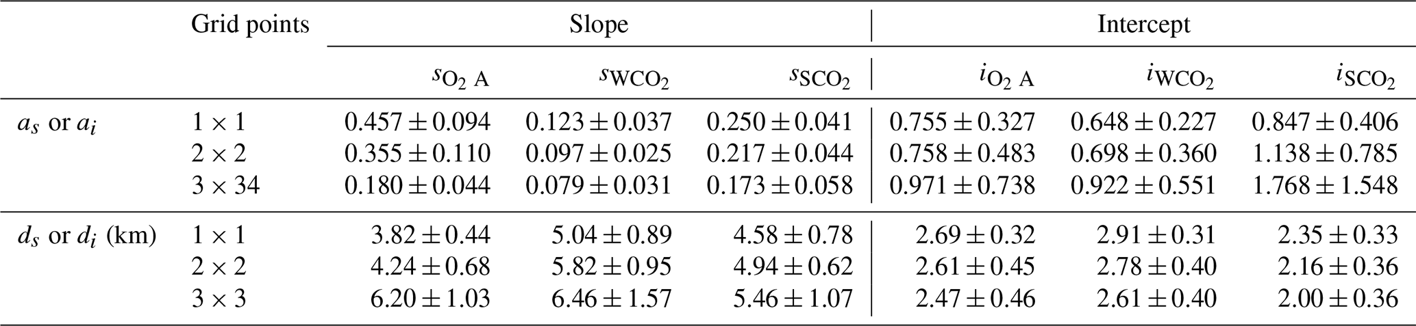
Since the OCO instrument series have a narrow field of view (FOV), 1.3 km × 2.3 km compared to 78 km² (10.5 km in diameter) for the GOSAT series, the 3D cloud bias is considered more significant for the OCO retrieval when small footprints are in close proximity to clouds. Numerous upcoming satellites for CO₂ remote sensing will adopt similar retrieval algorithms but feature varying footprint sizes in accordance with their specific mission objectives. For example, the Copernicus Anthropogenic CO2 Monitoring Mission (CO2M) by the European Space Agency (ESA) plans to have a footprint size of 4 km² (2 km by 2 km; Kuhlmann et al., 2020). MicroCarb by the Centre National d'Etudes Spatiales (CNES) will have a larger footprint size of 40.5 km² (4.5 km by 9 km; Cansot et al., 2023). Thus, exploring the influence of footprint size on 3D-effect parameters is vital. We performed an analysis analogous to the one described in Sect. 5.3 but expanded the average domain from the closest 5 × 5 grid points (approximately 1 × 1 km²) to 9 × 9 and 13 × 13 grid points (approximately 2 × 2 and 3 × 3 km²). Figure A5 displays the updated distributions of s and i. The s and i and cloud distance fitting results in the bypass method, presented in Table 3, indicate a decrease in a_s across all three bands. This decline aligns with the expectation that larger footprints would mitigate the spectral distortion effect, reducing the prevalence of the 3D cloud biases. No statistically significant change exists in a_i and d_i in the intercept values across different footprint sizes.

In addition, d_s exhibit an increase compared to the smaller footprint size. This implies that even though the baseline radiance change may demonstrate a minor deviation compared to the 1D-RT simulation as the footprint size expands, the perturbation difference in relation to reflectance might persist due to the increasing d_s. We suggest that future satellite missions, regardless of footprint size, consider accounting for 3D biases to improve the accuracy of X${}_{{\mathrm{CO}}_{\mathrm{2}}}$ retrievals. Studies need to be conducted to ensure that, given the bands, footprint size, and other attributes, the retrieval error induced by 3D clouds does not exceed the mission requirements – similar to what has been demonstrated for OCO-2 in this study. For missions utilizing larger footprint sizes to achieve broader global coverage, the 3D cloud effect may be diminished but distributed over a more extensive area. Conversely, missions designed with smaller footprint sizes than OCO-2, particularly those targeting enhanced data acquisition in cloud-prone regions such as the Amazon basin – where land nadir observations have been reported to exhibit biases up to −0.48 ppm in both hemispheres (Massie et al., 2023) – must rigorously account for 3D radiative transfer effects. While new missions may propose alternative retrieval algorithms, such as leveraging a reference gas with an absorption band adjacent to the CO₂ band (Frankenberg et al., 2024), these approaches require thorough validation. Therefore, it is imperative that such missions integrate robust 3D-RT mitigation strategies, such as those proposed in Sect. 5.6, into their design and planning phases to ensure compliance with mission requirements.

Table 3 Amplitude and e-folding distances for s and i, determined using different average grid points in simulations with a homogeneous aerosol layer for the O₂ A, WCO₂, and SCO₂ bands. Errors represent fitting uncertainty only and may be underestimated.

5.5 Impact of solar zenith angle and surface reflectance

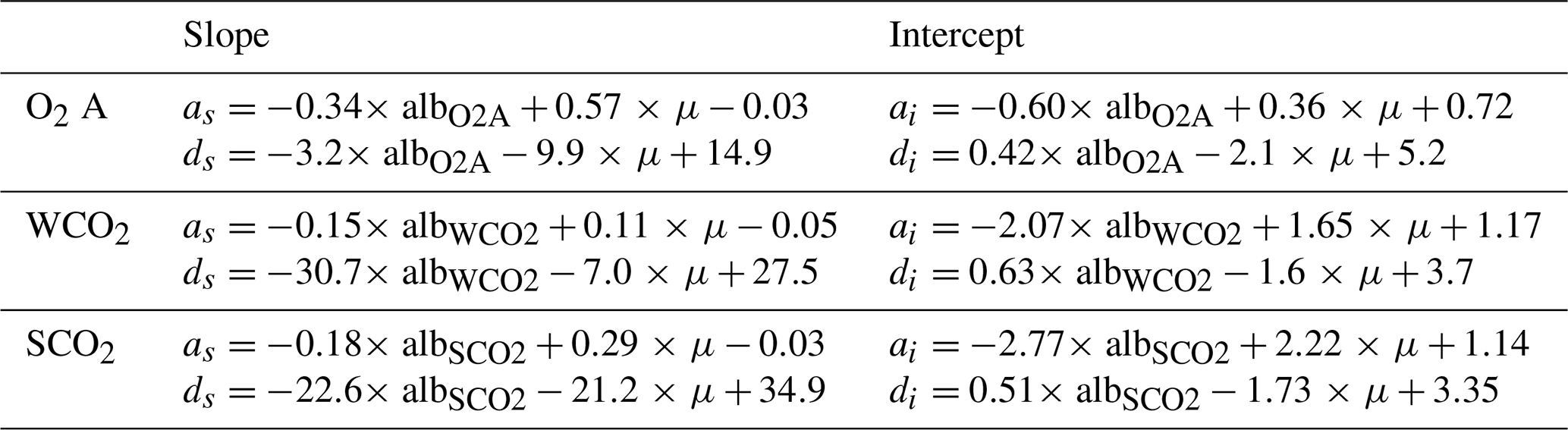
Solar zenith angle and surface albedo are significant factors influencing the 3D cloud effect, represented by a parameterized set of 12 relationships. To investigate their impact on the 3D cloud effect, we also kept several variables constant, including COT, CER, CTH, cloud position, AOD, and atmospheric conditions, the setup used in Sect. 5.3, and manually changed the SZA and surface reflectance. Figures A5 and A6 illustrate how these variables impact the 3D cloud effect in the O₂ A-band under different conditions. Combining results across various solar zenith angles and surface albedo values, we developed a two-variable linear parameterization using a_s and d_s (slope parameters) and a_i and d_i (intercept parameters). As summarized in Table 4, we observe that the amplitude of the slope and intercept is inversely proportional to surface albedo and directly proportional to the cosine of the solar zenith angle (denoted μ). Additionally, the e-folding distances of the slope (d_s) are negatively proportional to both surface albedo and μ, while those of the intercept are positively proportional to surface albedo and negatively proportional to μ. In general, higher surface albedo reduces the 3D cloud effect, as additional photons reaching the sensor represent a smaller fraction of the total signal. Conversely, lower solar zenith angles result in a smaller amplitude but longer e-folding distance, causing the 3D effect to extend further from the clouds.

Table 4 The parameterization of a_s and d_s of the slope and a_i and d_i of the intercept for the three OCO-2 bands. Errors represent fitting uncertainty only and may be underestimated.

5.6 3D-effect mitigation

Utilizing the derived s and i for the 3D effect, we can mitigate the associated biases through the “radiance adjustment” process, as elaborated in Sect. 4.4. The assumption is that the 3D effect is removed in the adjusted 1D radiance, allowing us to retrieve the mitigated X${}_{{\mathrm{CO}}_{\mathrm{2}}}$ using existing operational retrieval algorithms. To mitigate the 3D biases in X${}_{{\mathrm{CO}}_{\mathrm{2}}}$, it is essential to compute the 3D parameters (s and i for the three OCO-2 spectral bands) for all footprints that pass the prescreening (quality flag =0 or 1).

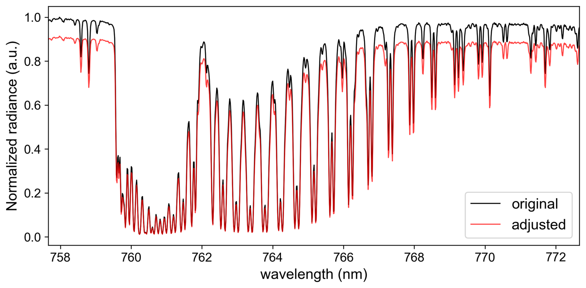
Both the baseline and bypass methods rely on the same mitigation framework but differ in how s and i are obtained for each footprint. In the baseline method, 3D-RT simulations are performed on a per-pixel basis to directly obtain s and i. By contrast, the bypass method first calculates D_e for each footprint based on the cloud position, incorporating parallax and wind correction (refer to Fig. A4 as an example), and then uses the exponential-fit coefficients in Table 2 to map D_e to s and i. Finally, the adjusted spectra are derived for both methods in accordance with Eq. (4). Figure 8 presents an example of the original and corresponding adjusted spectra of the O₂ A-band. In this study, we demonstrate the integration of our mitigation framework into current operational retrieval algorithms to effectively reduce the 3D cloud bias.

Figure 8 Example of an O₂ A spectrum before and after radiance adjustment.

Using the B10.04 retrieval algorithm (refer to Sect. 4.4), we calculate the newly retrieved X${}_{{\mathrm{CO}}_{\mathrm{2}}}$ values for each footprint. Figure 9 displays the distribution of retrieved X${}_{{\mathrm{CO}}_{\mathrm{2}}}$ before and after the spectral adjustment, superimposed on the collocated MODIS Aqua image. The elevated X${}_{{\mathrm{CO}}_{\mathrm{2}}}$ near the cloud decreases after the adjustment approximation, with the newly retrieved X${}_{{\mathrm{CO}}_{\mathrm{2}}}$ values reduced by approximately 0 to 3 ppm for D_e greater than 5 km and by more than 3 ppm for D_e less than 5 km. A comparison of ΔX${}_{{\mathrm{CO}}_{\mathrm{2}}}$ (the newly retrieved X${}_{{\mathrm{CO}}_{\mathrm{2}}}$ minus the original L2 value) against D_e is presented in Fig. 10 for both methods. Both methods exhibit analogous ΔX${}_{{\mathrm{CO}}_{\mathrm{2}}}$ patterns and offer similar average reductions. Specifically, the bypass method registers an average ΔX${}_{{\mathrm{CO}}_{\mathrm{2}}}$ of −0.778 ppm, in contrast to the baseline method, which delineates an average ΔX${}_{{\mathrm{CO}}_{\mathrm{2}}}$ of −0.876 ppm. The observed variance of ΔX${}_{{\mathrm{CO}}_{\mathrm{2}}}$ potentially emanates from simplified assumptions in the bypass method. Larger biases near cloud edges are captured more accurately by the baseline method, but both approaches confirm that the bias diminishes with increasing cloud distance.

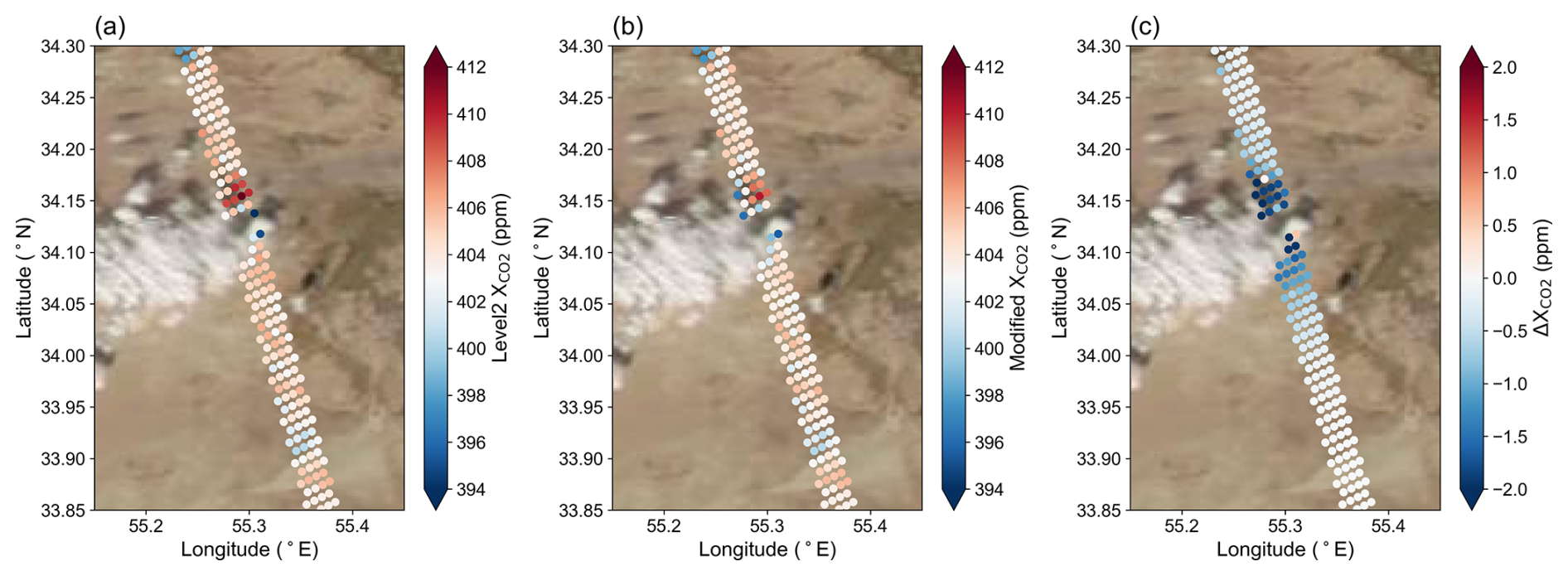
Figure 9 Satellite true-color imagery of MODIS Aqua from NASA Worldview on 18 October 2018 with (a) X${}_{{\mathrm{CO}}_{\mathrm{2}}}$ in OCO-2 Level 2 data, (b) mitigated X${}_{{\mathrm{CO}}_{\mathrm{2}}}$ retrieved from the adjusted spectra, and (c) the difference between the mitigated and original X${}_{{\mathrm{CO}}_{\mathrm{2}}}$ values.

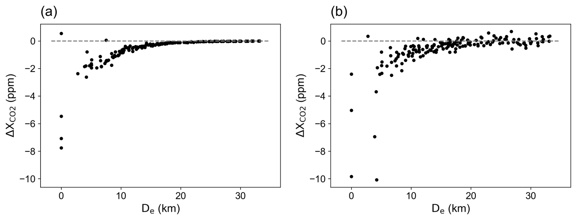
Figure 10 (a) Relationship of ΔX${}_{{\mathrm{CO}}_{\mathrm{2}}}$ with D_e as depicted in Fig. 7c based on parameterized slopes and intercepts from the bypass method. ΔX${}_{{\mathrm{CO}}_{\mathrm{2}}}$ is defined as the difference between the newly retrieved X${}_{{\mathrm{CO}}_{\mathrm{2}}}$ and Level 2 X${}_{{\mathrm{CO}}_{\mathrm{2}}}$. (b) Corresponding relationship using slopes and intercepts derived from the baseline approach.

The goal of the OCO-2 mission is to determine X${}_{{\mathrm{CO}}_{\mathrm{2}}}$ uncertainty to within 1 ppm. Setting the true mixing ratio to the mean X${}_{{\mathrm{CO}}_{\mathrm{2}}}$ for an effective distance exceeding 15 km, we see that X${}_{{\mathrm{CO}}_{\mathrm{2}}}$ scatter is accentuated within 15 km of clouds, as demarcated by the black markers in Fig. 11a. The mitigated X${}_{{\mathrm{CO}}_{\mathrm{2}}}$ after the spectra adjustment, represented by the red markers in Fig. 11a, exhibits reduced scatter within 15 km of clouds, a fact further corroborated by the full width at half maximum (FWHM) depicted in Fig. 11b. Cumulatively, the bypass method aligns favorably with the baseline methodology, offering the added benefit of small computational demands. Our physically based adjustment thus achieves 3D bias reduction near clouds at the radiance level for the first time, while still allowing the use of the original 1D retrieval code.

The processing time per footprint for the baseline analysis is approximately 7 min when using 32 CPUs (AMD EPYC Processor 7713) on a cluster to simulate 1 × 10⁹ photons for the full experimental domain. This is contrasted with the standard retrieval time of roughly 2.5 min per footprint using 16 CPUs (Intel Xeon Processor E5-2623 v3) on a local workstation. Although the 3D computation time of 7 min marks a significant improvement over full-spectra 3D simulation, the additional 3D-RT calculations required to account for the missing physics could extend the duration to nearly 6 times that of a standard retrieval on a per-footprint, per-CPU basis. The bypass method offers a pragmatic alternative to mitigating the 3D cloud effect for large-scale applications while conserving computational resources. This method can be supplemented by periodic full calculations to increase the accuracy of the bypass approach but needs to be tested on a larger dataset before further application.

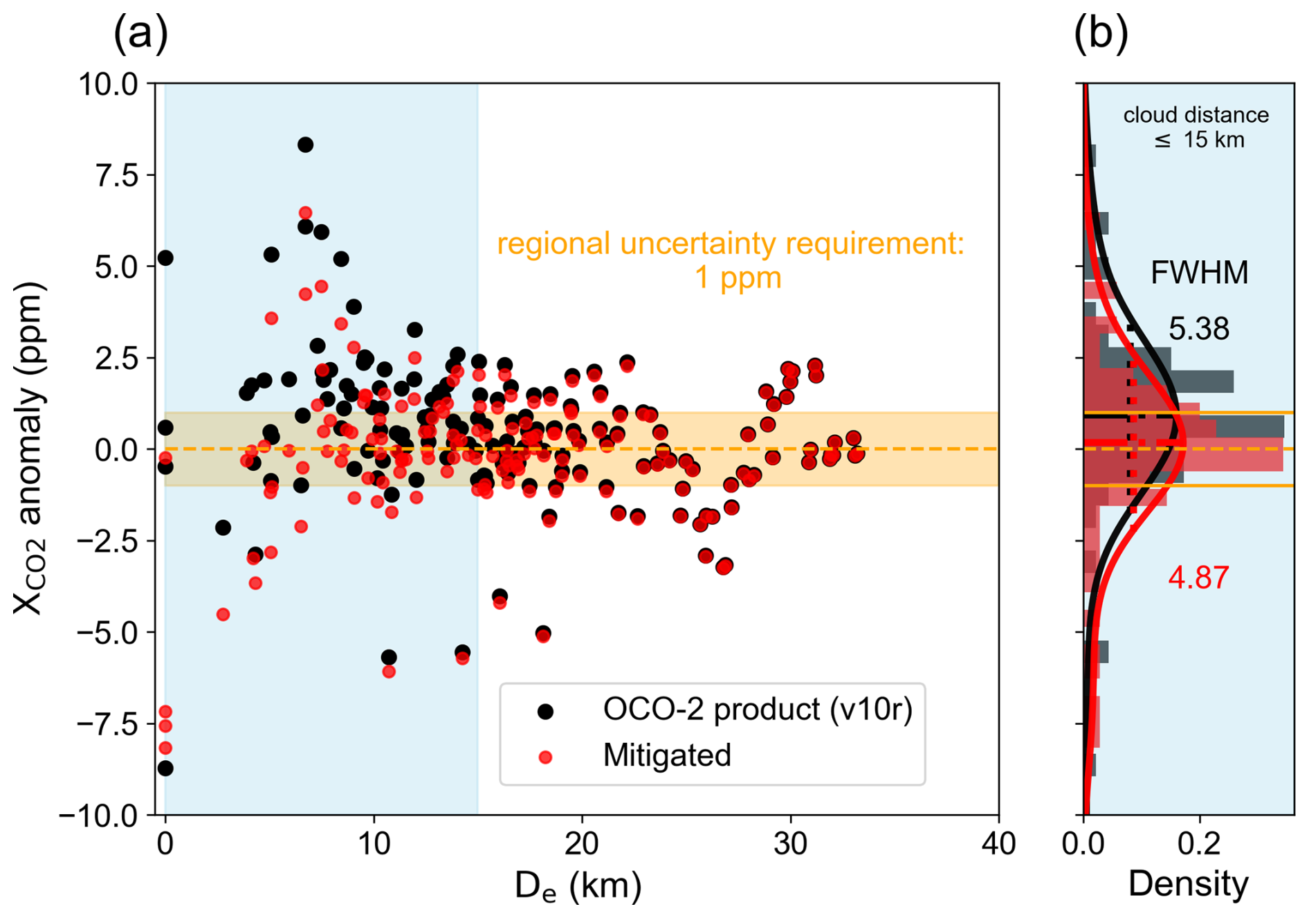
Figure 11 (a) Scatterplot comparing the X${}_{{\mathrm{CO}}_{\mathrm{2}}}$ anomaly of the OCO-2 L2 product (in black) to its value post-spectra adjustment (in red), plotted against D_e. The X${}_{{\mathrm{CO}}_{\mathrm{2}}}$ anomaly is defined as retrieved X${}_{{\mathrm{CO}}_{\mathrm{2}}}$ – true X${}_{{\mathrm{CO}}_{\mathrm{2}}}$, with the true X${}_{{\mathrm{CO}}_{\mathrm{2}}}$ defined by the average X${}_{{\mathrm{CO}}_{\mathrm{2}}}$ of footprints with a D_e greater than 15 km (403.714 ppm in this case). The orange shade indicates the 1 ppm mission requirement. (b) Histograms and probability density functions (PDFs) for the X${}_{{\mathrm{CO}}_{\mathrm{2}}}$ anomaly of the OCO-2 L2 product (in black) and post-spectra adjustment (in red) within a 15 km D_e. This corresponds to the blue-shaded region in (a). The FWHM values of the PDFs of v10r and adjusted data points are 5.38 and 4.87, and the PDF averages are 0.796 and −0.178, respectively. The average change in X${}_{{\mathrm{CO}}_{\mathrm{2}}}$ after the spectra adjustment for D_e less than 15 km is −1.131 ppm.

To evaluate the applicability of the bypass approach, we applied the parameter set in Table 2 to another scene (Fig. A7a) from the same month and a nearby region. We also conducted a baseline 3D-RT simulation for direct comparison (Fig. A8). The results indicate that the bypass method follows a trend similar to the baseline method, although with smaller mitigation magnitudes. Differences between the two (Fig. 9) are likely due to variations in surface altitude, albedo, solar geometry, AOD, and other factors. Although promising, the bypass approach may benefit from additional tuning to account for these scene variables. However, it can be less effective under complex cloud–surface conditions.

6 Conclusions

This research uses the EaR³T-OCO radiance simulator, which considers the scene context of givens, to evaluate and mitigate the impact of missing physics in the context-agnostic operational retrieval that stems from clouds in the vicinity of an OCO-2 sounding. We then used the simulator to undo the effects of such clouds by reversing the perturbations relative to the clear sky that were exerted on the observed radiances. In essence, the observed radiance spectra were mapped back to what they would have been in the absence of clouds in the vicinity of a footprint. This radiance mapping is done based on the difference between simulated 1D and 3D radiance calculations (3D perturbations). After this mapping, the standard X${}_{{\mathrm{CO}}_{\mathrm{2}}}$ retrieval can then be applied. In this way, we introduced a physics-based mitigation of 3D-RT effects on trace gas spectroscopy products, previously regarded as intractable for real-world applications such as this.

To avoid “brute-force” computing full-spectrum 3D effects, we introduced a physics-based acceleration approach with only a few representative wavelengths. The resulting 3D perturbations are encapsulated by 12 linear fit parameters (slope and offset), reducing the complexity of the correction. This acceleration method is distinct from previously published methods, including approaches to “freeze” photon paths for various wavelengths (Emde et al., 2011; Iwabuchi and Okamura, 2017). The spectral perturbation parameters can also be linked to macroscopic scene parameters to analyze their influence on 3D cloud effects. If successful, this method could bypass 3D-RT calculations altogether while retaining the core physics. By applying this bypass parameterization approach, the mitigation of cloud effects at the radiance level becomes feasible for operational applications, offering a stronger physical foundation compared to statistical mitigation methods and enabling broad applicability to OCO-2 and 3 and other spectroscopy missions that have collocated imagery. Although further validation is required for a wider diversity of scenes, including variations in cloud top height, cloud morphology, aerosols, and different viewing modes, the linear perturbation representation and our mitigation framework approach account for the principal drivers of 3D cloud effects. Moreover, it highlights the fact that aerosols and footprint size can influence the magnitude of the 3D cloud effect, especially for future satellites such as MicroCarb, CO2M, and GOSAT-GW. In general, our research elucidates the 3D cloud perturbation on spectroscopy with high spectral resolution (trace gas retrievals) as opposed to spectrometry (cloud and aerosol imagery retrievals), where 3D effects are traditionally studied more extensively. Addressing these effects at the radiance level is suggested because that is where the operational standard 1D retrievals lack the necessary physics. We also understand that the effects are spectrally dependent, with cloud morphology, band-specific surface reflectance, and aerosol properties acting as the primary drivers. Our work can become the stepping stone toward more accurate and efficient trace gas retrievals in the vicinity of clouds. Looking ahead, adapting this mitigation to operational workflows could markedly improve X${}_{{\mathrm{CO}}_{\mathrm{2}}}$ accuracy in cloud-prone regions – including the Amazon – and thereby enhance the fidelity of CO₂ flux inversions.

7 Future work

This research emphasizes the substantial impact of aerosols, solar zenith angles, and surface albedo on the 3D-effect parameters of the three OCO bands. Concurrently, cloud properties emerge as critical determinants of these 3D-effect parameters. With additional simulations, there is an opportunity to incorporate the impacts of various factors into the existing parameterization framework. The current investigation concentrates on scenarios over land in nadir mode. We will develop a similar parameterization (as in Table 3) for ocean and land in glint mode.

Appendix A: Supplementary figures

Appendix A contains supplementary information to complement the details of the simulation setting. These elements cover various topics, from atmospheric profiles and cloud-related parameters to radiative transfer simulations.

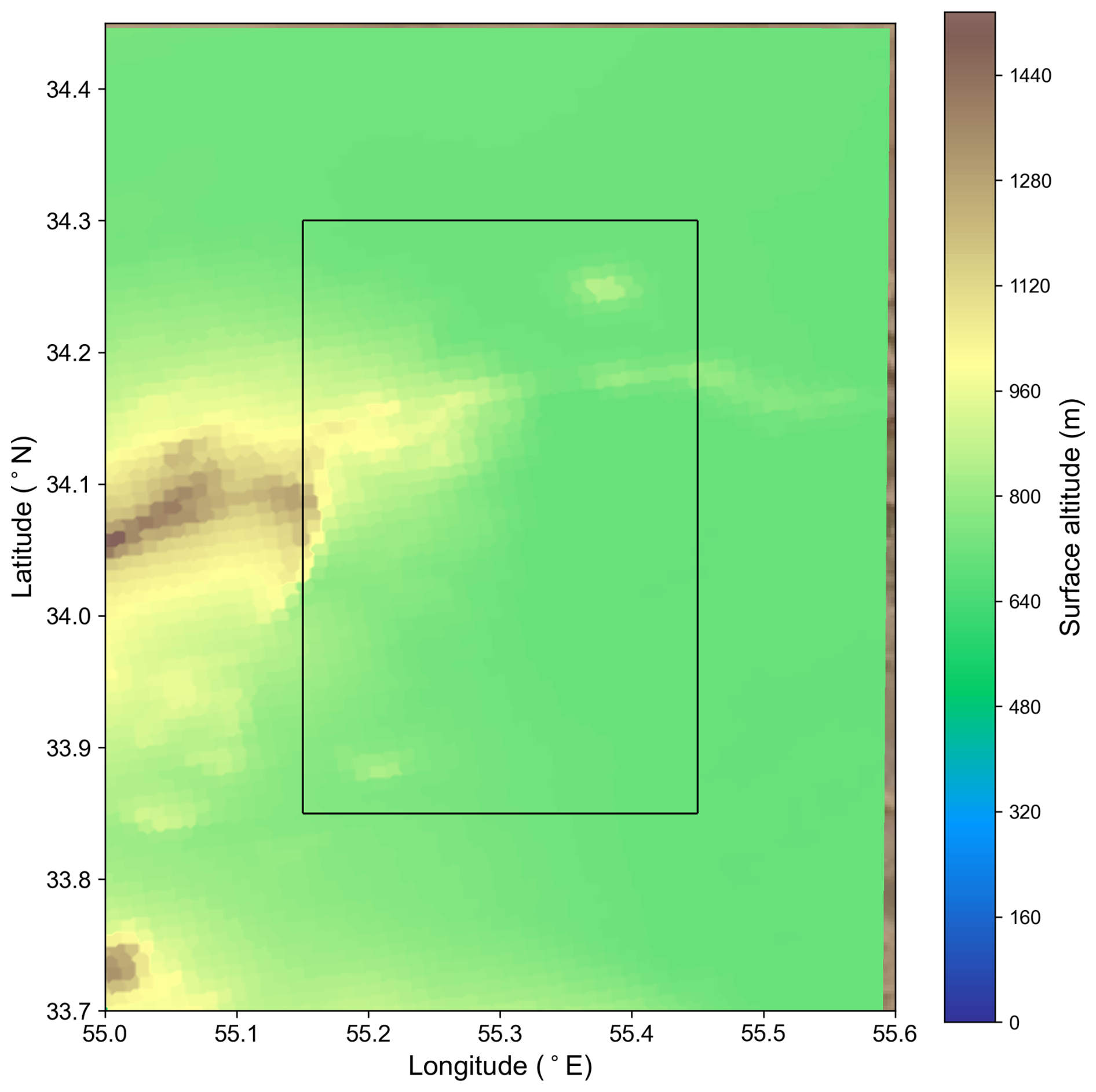
Figure A1 Contour plot showcasing surface height from the MODIS MYD03 file for the outer simulation domain and the inner analysis domain.

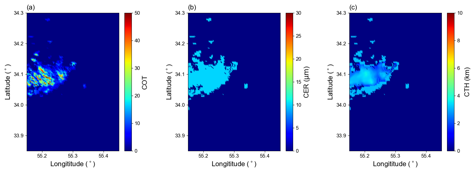
Figure A2 The cloud optical thickness (a), cloud liquid effective radius (b), and cloud top height (c) for the 3D simulation at 650 nm.

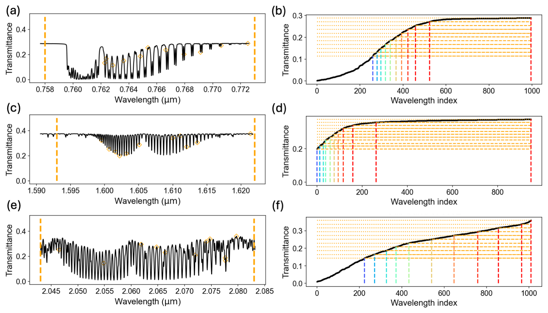
Figure A3 Simulated transmittance of (a) O₂ A, (c) WCO₂, and (e) SCO₂ bands derived from the atmospheric structure presented in Fig. B1. The right panels present the sorted transmittance with the selected wavelength index for (b) O₂ A, (d) WCO₂, and (f) SCO₂ bands. The orange markers on the left panels denote the corresponding selected wavelengths shown in the right panels.

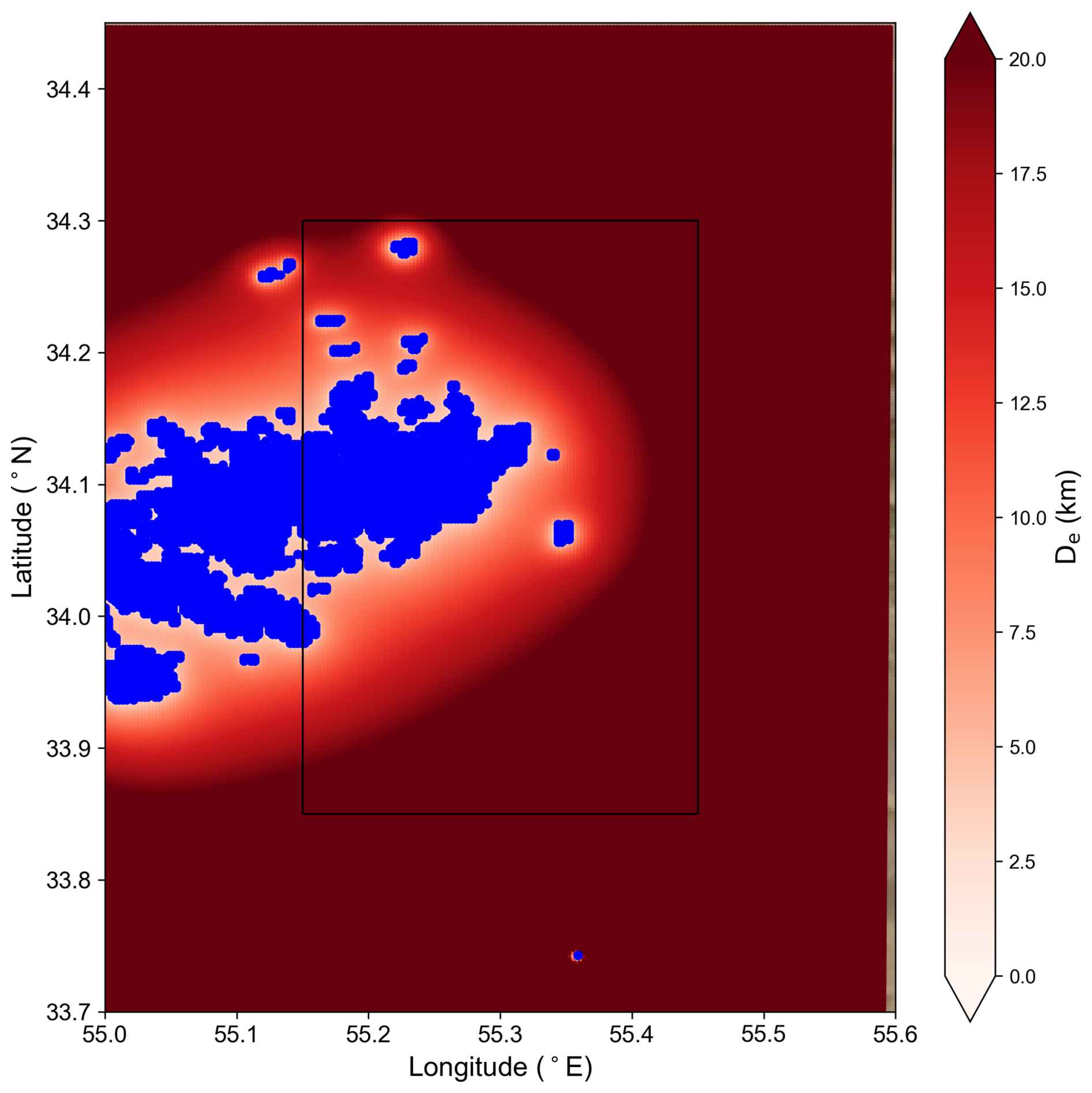
Figure A4 Distribution of the effective cloud distance, with blue dots marking the positions of the clouds. The black rectangle designates the analysis domain, while the entire domain represents the region of the RT simulation.

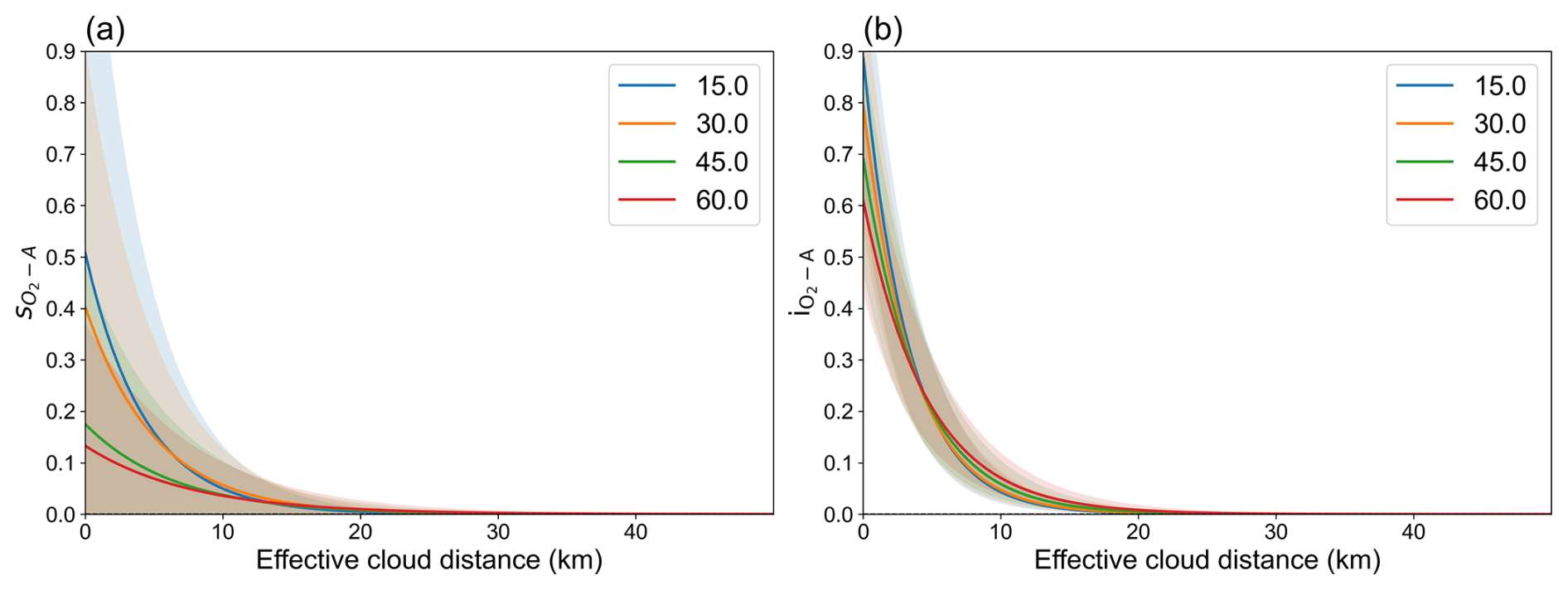
Figure A5 Parameterization of (a) slope and (b) intercept for the O₂ A band with effective cloud distance, varied by solar zenith angle, while holding surface albedo constant.

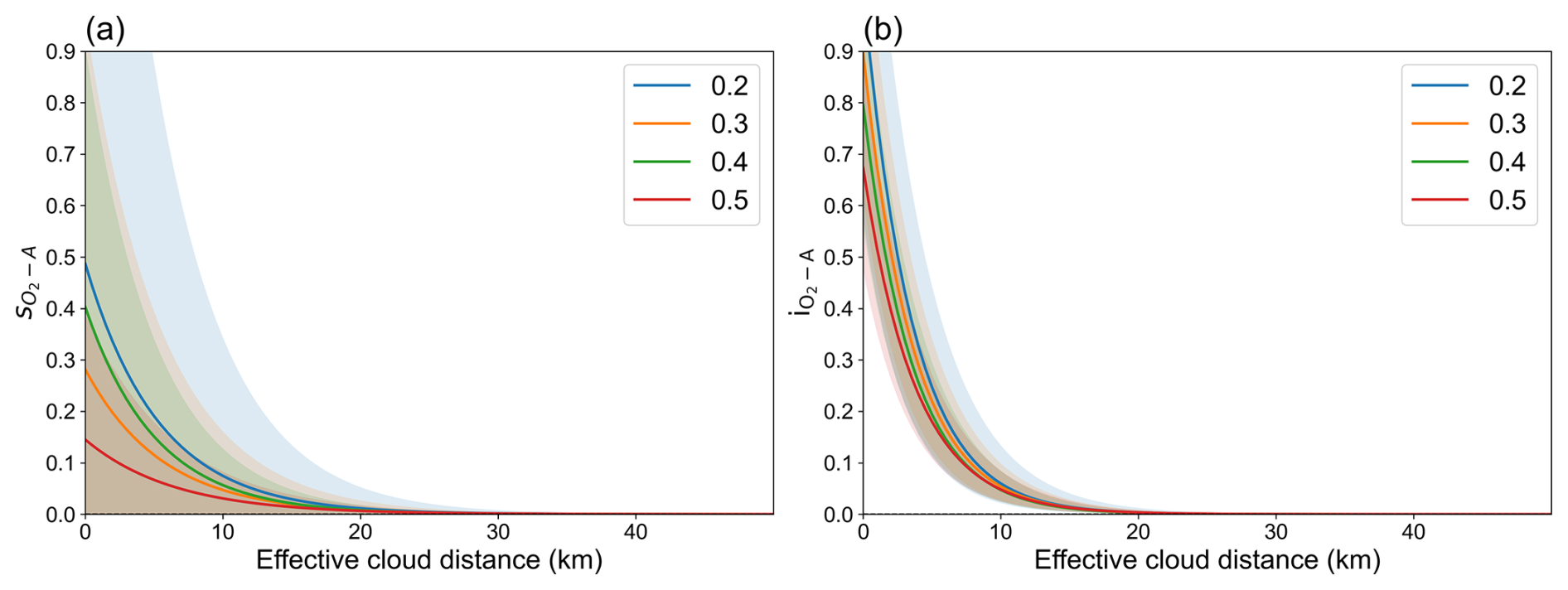
Figure A6 Parameterization of (a) slope and (b) intercept for the O₂ A band with effective cloud distance, varied by surface albedo, while holding solar zenith angle constant.

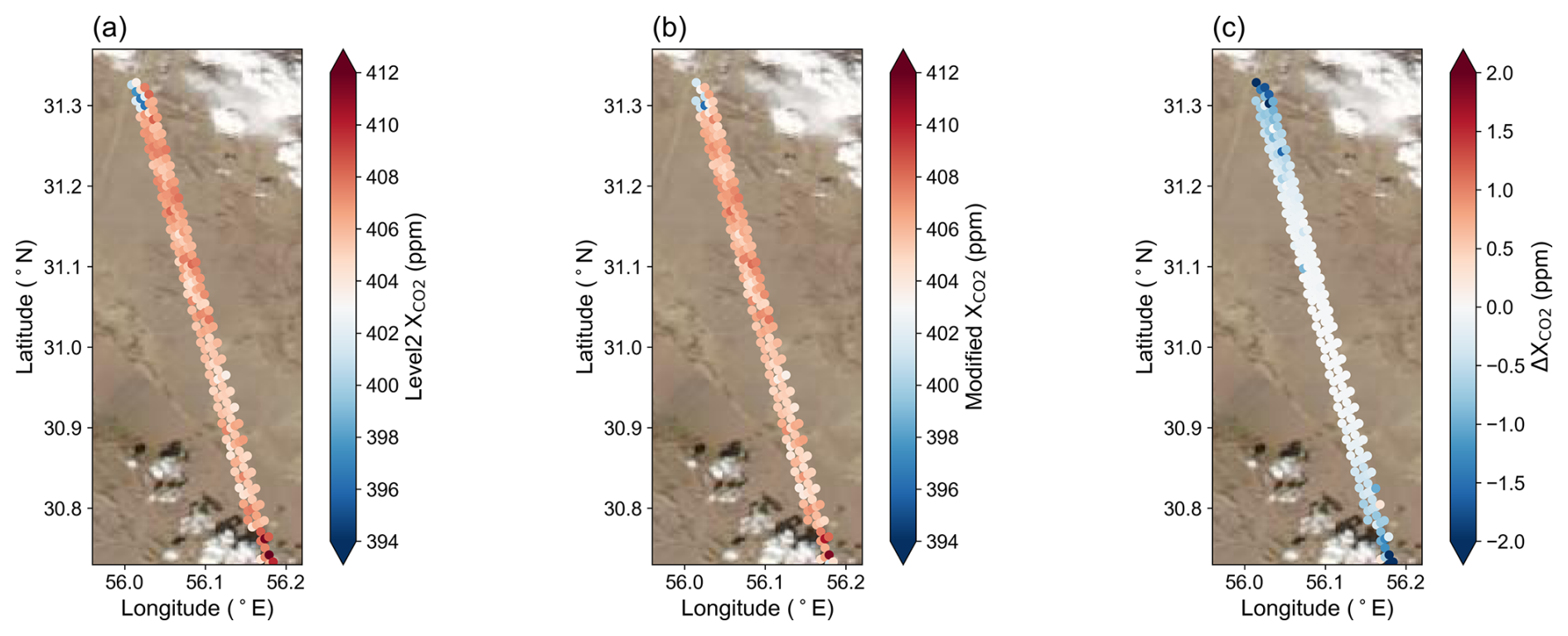
Figure A7 Satellite true-color imagery of MODIS Aqua from NASA Worldview on 5 October 2019 with (a) X${}_{{\mathrm{CO}}_{\mathrm{2}}}$ in OCO-2 Level 2 data, (b) mitigated X${}_{{\mathrm{CO}}_{\mathrm{2}}}$ retrieved from the adjusted spectra, and (c) the difference between the mitigated and original X${}_{{\mathrm{CO}}_{\mathrm{2}}}$ values.

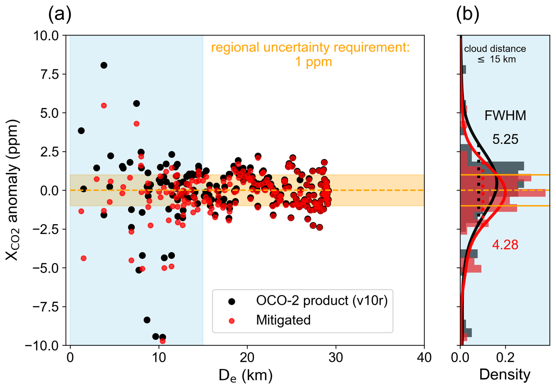
Figure A8 (a) Scatterplot comparing the X${}_{{\mathrm{CO}}_{\mathrm{2}}}$ anomaly of the OCO-2 L2 product (in black) to its value post-spectra adjustment (in red) for the case shown in the figure above, plotted against D_e. The X${}_{{\mathrm{CO}}_{\mathrm{2}}}$ anomaly is defined as retrieved X${}_{{\mathrm{CO}}_{\mathrm{2}}}$ – true X${}_{{\mathrm{CO}}_{\mathrm{2}}}$, with the true X${}_{{\mathrm{CO}}_{\mathrm{2}}}$ defined by the average X${}_{{\mathrm{CO}}_{\mathrm{2}}}$ of footprints with an _e greater than 15 km (405.96 ppm in this case). The orange shade indicates the 1 ppm mission requirement. (b) Histograms and probability density functions (PDFs) for the X${}_{{\mathrm{CO}}_{\mathrm{2}}}$ anomaly of the OCO-2 L2 product (in black) and post-spectra adjustment (in red) for D_e within 15 km. This corresponds to the blue-shaded region in (a). The FWHM values of the PDFs of v10r and adjusted data points are 5.25 and 4.28, and the PDF averages are 0.93 and 0.18, respectively. The average change in X${}_{{\mathrm{CO}}_{\mathrm{2}}}$ after the spectra adjustment for D_e less than 15 km is −0.86 ppm.

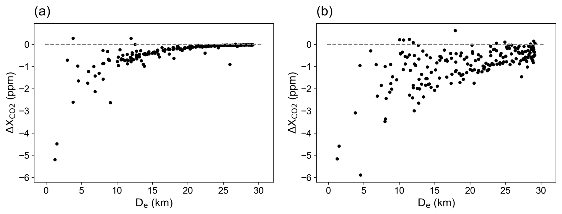
Figure A9 (a) Relationship of ΔX${}_{{\mathrm{CO}}_{\mathrm{2}}}$ with D_e based on parameterized slopes and intercepts from the bypass method in Table 2. (b) The corresponding relationship using slopes and intercepts derived from the baseline approach for Fig. A7.

Appendix B: Radiative transfer simulations

B1 Vertical atmospheric structure

The atmosphere profile for the simulation is constructed based on the OCO-2 Met and CO₂ prior data, and it is vertically divided into 29 layers. The surface altitude and pressure are determined by the average surface height of the footprints analyzed. The heights of the other layers are then linearly interpolated from the surface to 5 km for 11 points, with 0.5 km intervals from 5 to 10 km, 1 km intervals from 10 to 14 km, and 5 km intervals from 20 to 40 km, which was the top height of the simulation. The pressure profile corresponding to these heights is calculated using a method similar that of to the MERRA-2 reanalysis product (Bosilovich et al., 2015) from NASA's Global Modeling Assimilation Office (GMAO). The temperature and horizontal wind profiles are then retrieved from the OCO-2 Met data by linear interpolation between pressure and temperature/wind.

Accurate number densities of O₂, CO₂, and water vapor are crucial for calculating the absorption coefficients. We assumed that the atmosphere followed the ideal gas law to estimate the number density of each layer. O₂ number density is determined by multiplying its dry-air mixing ratio (0.20935; OCO-2 L2 ATBD, 2021) with the dry-air number density. CO₂ number density is calculated similarly by using the CO₂ prior profile. We use the specific humidity in the OCO-2 Met data as well as the temperature and pressure to derive the water vapor volume mixing ratio (VMR) profile. H₂O VMR is essential to obtain more accurate absorption coefficients to consider the water vapor broadening, which is discussed further in Appendix B2. The H₂O VMR profile is also converted into number density for further absorption calculation. The derived profiles are displayed in Fig. B1. These steps ensure that the atmospheric parameters used in the simulation are as accurate as possible.

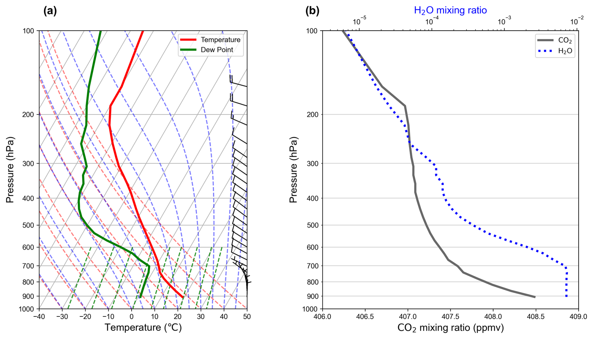
Figure B1 (a) Skew-T diagram of the atmosphere and (b) CO₂ and H₂O VMR profiles of the Fig. 1 scene.

B2 Absorption coefficients

For missions with high spectral resolution, such as GOSAT and OCO, accurate absorption coefficients within the observed range are indispensable for meticulously modeling the absorption process. This study utilizes the same precalculated lookup tables of absorption coefficients (ABSCO tables) employed in version 10 of the OCO retrieval algorithm (ABSCO V5.1, Payne et al., 2020). These ABSCO tables furnish line-by-line absorption cross-sections for O₂, CO₂, and H₂O within the observed wavelength range. They also account for line mixing, speed dependence of molecular collisions, and collision-induced absorption (OCO L2 ATBD, 2021). Due to the design of OCO instruments and the varying viewing angles of the eight footprints within the same swath, the wavelengths of each band exhibit slight discrepancies (OCO L1B ATBD, 2021). To mitigate excessive computational demands, we opt to use solely the wavelengths of the first footprint.

The ABSCO tables are functions of the pressure, temperature, and water H₂O VMR. Because the grid points of pressure, temperature, and H₂O VMR are discrete, we calculate the absorption coefficients by applying trilinear interpolation to approximate the cross-section of each line. The instrument line shape provided in the OCO L1B file was used to weigh various lines when calculating the absorption coefficient for each wavelength. With the molecule number densities of O₂, CO₂, and water vapor established during the step in Appendix B1, we compute the absorption coefficients in km⁻¹ for O₂ A, WCO₂, and SCO₂ for lines whose relative cross-sections exceeded 0.05 compared to the largest within the instrument line shape range. The clear-sky transmittance for each wavelength can be calculated using the derived absorption coefficients.

B3 Cloud detection and properties

MODIS products provide cloud mask information with a cloud identification accuracy of about 90 % over land between 60° N and 60° S (Frey et al., 2020). However, undetected clouds can lead to a significant radiance inconsistency in RT simulation for a small footprint. To address this, we detect clouds based on the reflectance difference between the observation and white-sky surface albedo provided by the MODIS 43 product. We use various reflectance thresholds for different cases to ensure that most clouds are detected. This cloud detection approach is distinct from the method used by Chen et al. (2023) and is specifically designed for this study.

Once the cloudy pixels are identified, we retrieve the cloud top height (CTH) of the nearest location from the MODIS MYD02 cloud file and assign it to each cloudy grid point. The cloud effective radius (CER) is manually set to 10 µm for low clouds and 25 µm for high clouds in this study. We plan to use the actual MODIS CER values in future versions to capture more realistic variations. To determine each pixel's cloud optical thickness (COT), we run the RT model over several COTs and derive the COT–radiance relationship by ourselves to ensure the radiance consistency in the 1D-RT simulation. The COT of each pixel is then determined by applying the COT–radiance relationship. To adjust for the projection and observation time difference between OCO-2 and MODIS Aqua, we apply a cloud position adjustment as described by Chen et al. (2023). The adjustment includes a geometry parallax shift in the cloud position due to the time shift, wind speed, and direction determined by CTH.

By necessity, this study assumes fixed cloud geometric thickness (1 km for cloud top heights smaller than 4 km and a cloud base at 3 km for cloud top heights greater than 4 km). The additional photon path caused by multiple scattering within clouds influences the magnitude of the 3D cloud effect, so the slopes are sensitive to the choice of geometric cloud thickness. Unfortunately, this parameter is not readily available from operational products. Some attempts are being made to exploit the O₂ A channel of OCO-2 (Zinner et al., 2019; Li and Yang, 2024). Once these are mature, the information will be used by our algorithm. Generally, since the vertical cloud properties can influence the magnitude and distribution of the 3D cloud effect, further investigation of the impact of cloud properties, including COT, CTH, and cloud base height, on the 3D cloud effect is recommended for future research.

B4 RT model and tools

This research uses a modified version of the Education and Research 3D Radiative Transfer Toolbox v0.1.1 (Chen et al., 2023) for OCO (EaR³T-OCO) to model the 1D and 3D radiances of the scene. The Monte Carlo Atmospheric Radiative Transfer Simulator version 0.10.4 (MCARaTS; Iwabuchi, 2006) serves as the core engine for this simulator, which automatically ingests satellite products and simulates 1D and 3D spectral radiances. MCARaTS iteratively traces the path of each photon and calculates the distribution of photons based on the final probability. Chen et al. (2023) demonstrate the ability of EaR³T to simulate the radiance observed by OCO-2. We utilize the framework and example application outlined in Chen et al. (2023) to develop a specialized version of the application, which is described in Appendix B. We improve the atmospheric structure based on the OCO-2 Level 2 products and the absorption coefficient derivation method, as described in Appendix B1 and B2. For the simulation of each wavelength, 1 × 10⁹ photons are used and distributed to various absorption lines for a single run. The mean radiance and the standard deviation are then calculated from three runs to estimate the uncertainty.

Appendix C: Code walk through

The code utilized for this study can be accessed from GitHub at https://github.com/ywchen-tw/OCO2 (last access: 29 January 2025). Subsequent sections specify the configuration file settings and provide an overview of the simulation and analysis process.

C1 Configuration file

The configuration file in CSV format controls the changeable parameters for the EaR³T-OCO simulation. The following table describes the meaning and data type of each variable. If a variable is not required to be specified, the default value is used.

Table C1 Comprehensive overview of configuration file parameters, including names, descriptions, data types, and requirements.

Figure C1 Workflow schematic of the preprocess function in the oco_simulation.py code.

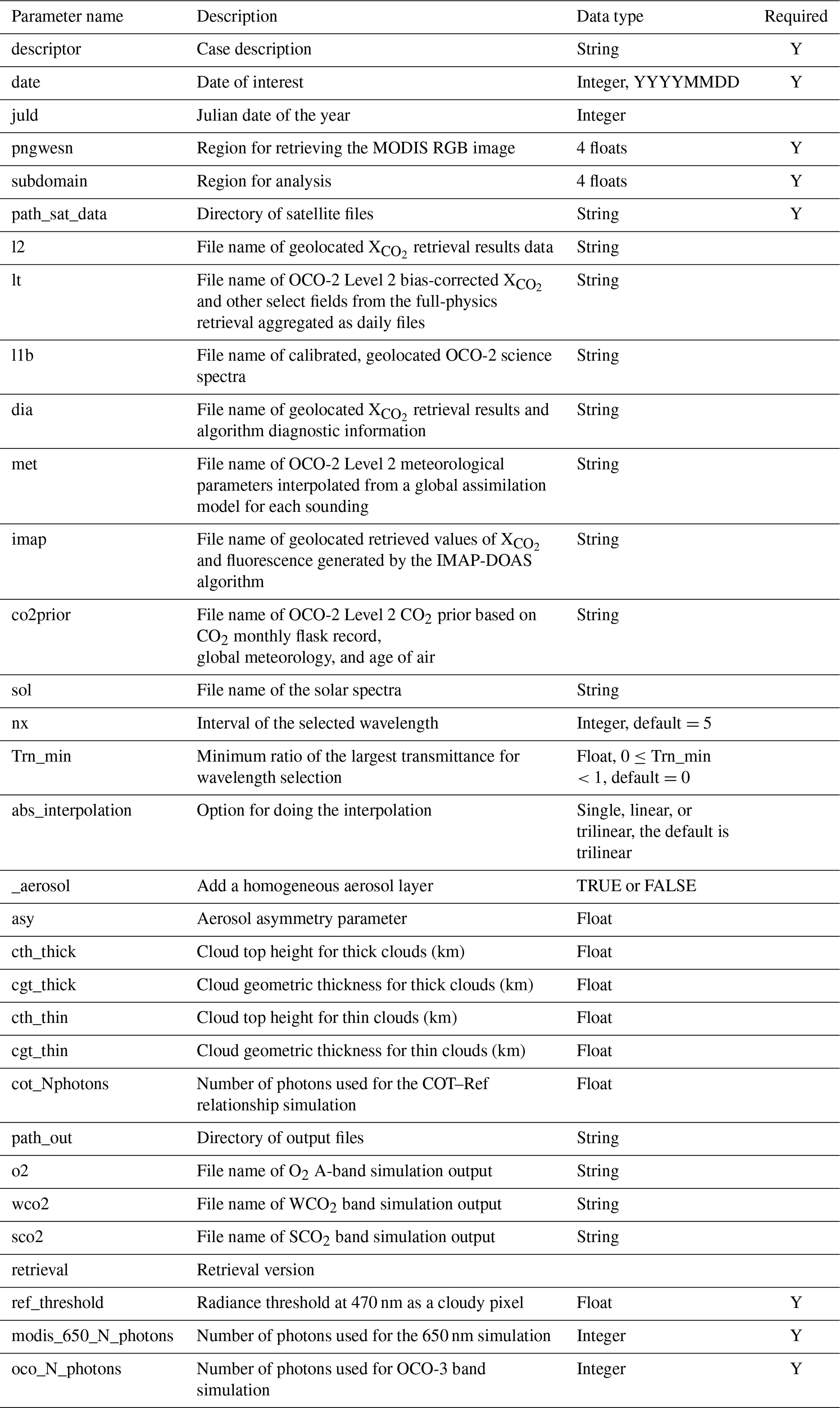
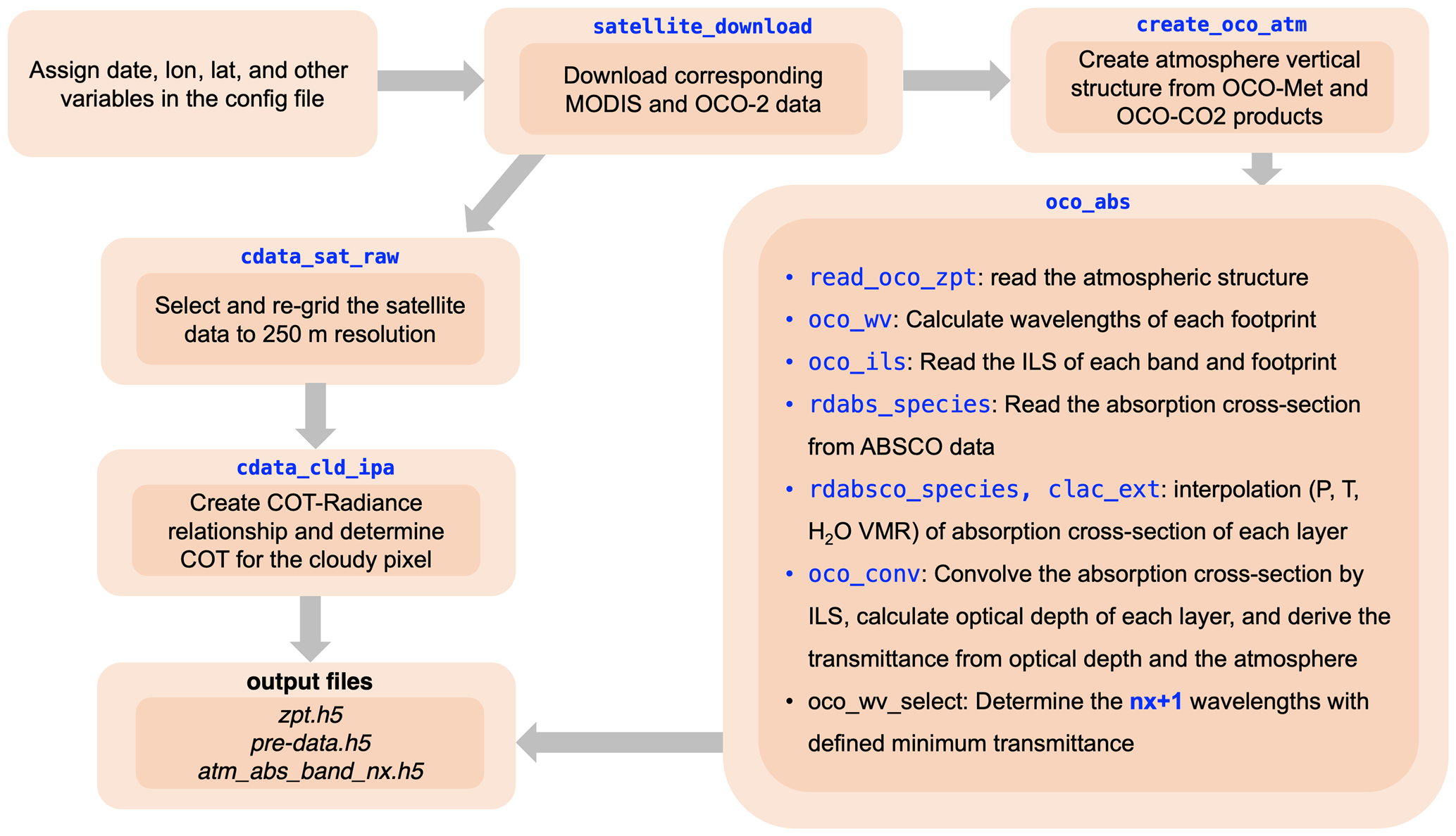
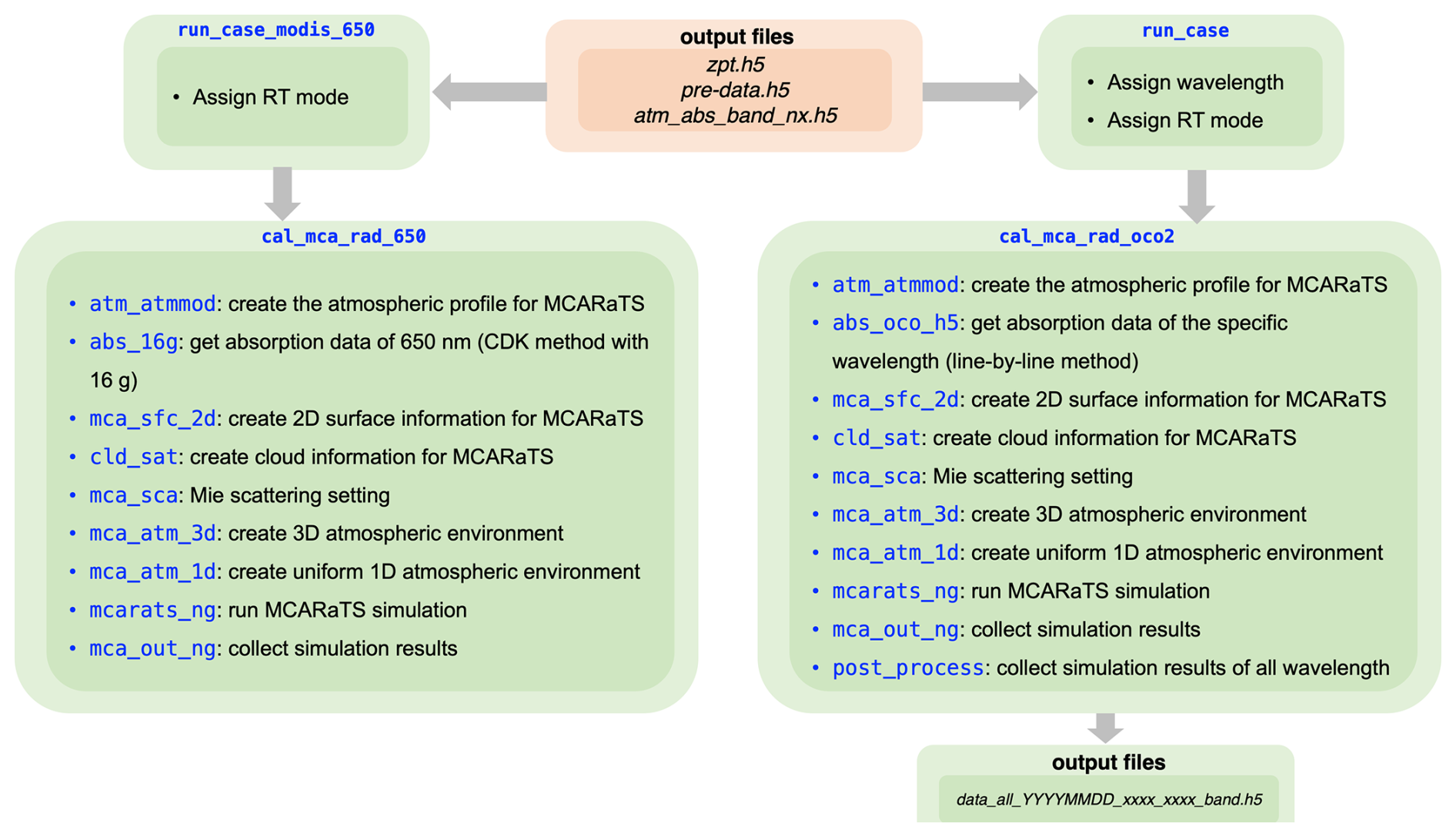
Figure C2 Workflow schematic of the run_case_modis and run_ case_oco functions in the oco_simulation.py code.

Figure C3 Workflow schematic of the case_analysis.py code and the oco_retrieve.py code.

C2 Preprocess

The oco_simulation.py code is the main code for data acquisition and radiance simulation. Here, we focus on the first part of the code (the preprocess function), which deals with data download and preprocessing.

1. satellite_download function. This function accesses the configuration file variables, subsequently downloading the pertinent MODIS and OCO-2 data as dictated by the specified date and geolocation details.

2. create_oco_atm function. Leveraging OCO-2 data, this function constructs vertical profiles for temperature, water vapor, and wind.

3. oco_abs function. Based on the atmospheric profiles, this function computes the optimal absorption coefficients for all three OCO-2 bands, subsequently identifying the wavelengths for simulation.

4. cdata_sat_raw function. This function extracts data from the MODIS and OCO-2 files, then restructures this data to a 250 m resolution.

5. cdata_cld_ipa function. Using the EaR³T simulator, this function establishes a COT–radiance relationship and designates a COT for every grid point.

Upon completion of the preprocessing stage, the system will generate the following files.

• zpt.h5. This file details the vertical atmospheric structure.

• pre-data.h5. This file contains information on cloud and radiance.

• atm_abs_band_nx.h5. This file captures data on the absorption coefficients.

C3 Simulation

The second part of the oco_simulation.py code (run_ case_modis and run_case_oco functions) is primarily concerned with radiance simulation.

1. run_case_modis function. This function drives the EaR³T simulator to simulate radiance at 650 nm, operating in either independent pixel approximation (IPA) or 3D mode. It employs the correlated k-distribution method, as detailed in Chen et al. (2023). Upon completion, simulation results are stored in the post_data.h5 file.

2. run_case_oco function. This function activates the EaR³T simulator to simulate radiance for each designated wavelength identified by the oco_abs function. It utilizes the IPA mode for clear-sky simulations and the 3D mode for real-world conditions. The respective simulation outcomes for each band are archived as data_all_YYYYMMDD_xxxx_ xxxx_band.h5.

C4 Postprocess

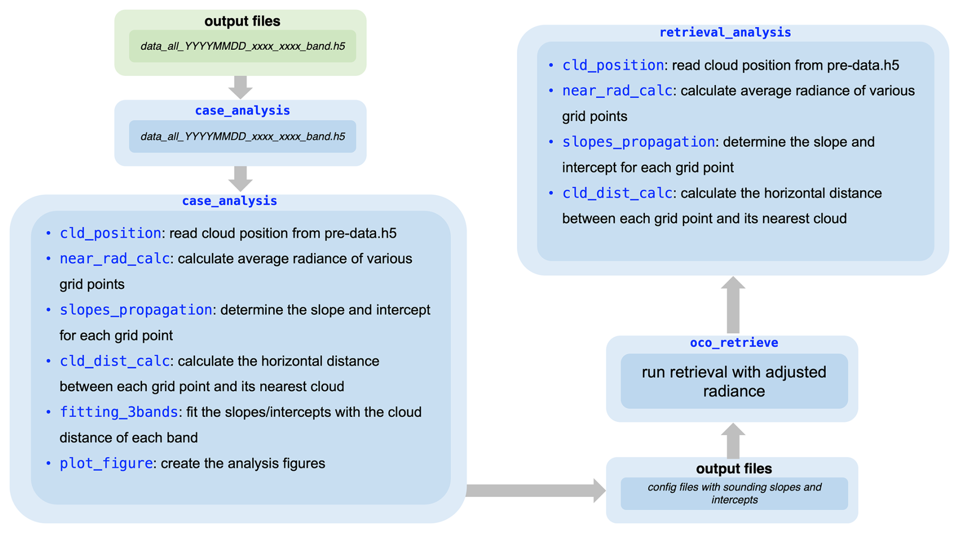
Following the radiance simulation, we proceeded with an analysis leveraging the case_analysis.py code and subsequently executed oco_retrieve.py to extract the mitigated X${}_{{\mathrm{CO}}_{\mathrm{2}}}$.

1. case_analysis function. This function accesses the output files from the radiance simulation and computes the mean radiance across various average sizes, a process managed by the near_rad_calc function. Next, the slopes_propagation function determines the slope and intercept for each grid point. With the help of the weighted_cld_dist_calc function, the effective cloud distance for each grid point is gauged based on cloud positioning. The fitting_3bands function determines the most suitable fitting coefficients for the 3D parameters and the effective cloud distance. Following this, the effective cloud distance for every footprint is established and used to derive the corresponding parameterized slopes and intercepts. All results are consolidated in the configuration file.

2. oco_retrieve function. Initially, this function adjusts the radiance of the footprint in line with the set slopes and intercepts. It then triggers the OCO retrieval algorithm with the modified spectra to obtain the mitigated X${}_{{\mathrm{CO}}_{\mathrm{2}}}$.

3. case_retrieval_analysis function. This function reviews the output of the mitigated X${}_{{\mathrm{CO}}_{\mathrm{2}}}$ and juxtaposes the findings with the OCO-2 L2 product.

Appendix D: Abbreviation

D1 Abbreviations and their full names in this paper

Abbreviation	Full name
A-train	Earth Observing System Afternoon
	Constellation
ABSCO	Absorption coefficients
AOD	Aerosol optical depth
CER	Cloud effective radius
CO2	Carbon dioxide
COT	Cloud optical thickness
CTH	Cloud top height
EaR3T	Education and Research 3D Radiative
	Transfer Toolbox
FOV	Field of view
FWHM	Full width at half maximum
GMAO	Global Modeling and Assimilation Office
GOSAT	Greenhouse Gases Observing Satellite
L (0,1...)	Level 0, Level 1, etc. (data product)
IPA	Independent pixel approximation
MCARaTS	Monte Carlo Atmospheric Radiative
	Transfer Simulator
MODIS	Moderate-Resolution Imaging
	Spectroradiometer
O2 A	Oxygen A-band
OCO	Orbiting Carbon Observatory
ppm	parts per million
R2	Determination coefficient
RT	Radiative transfer
SCO2	Strong CO2
TCCON	Total Carbon Column Observing Network
SZA	Solar zenith angle
TOA	Top of atmosphere
VMR	Volume mixing ratio
WCO2	Weak CO2
X${}_{{\mathrm{CO}}_{\mathrm{2}}}$	Column-averaged CO2 dry-air
	mole fraction