Improved consistency in solar-induced fluorescence retrievals from GOME-2A with the SIFTER v3 algorithm

Space-based observations of solar-induced fluorescence (SIF) provide valuable insights into vegetation activity over time. The GOME-2A instrument, in particular, facilitates SIF retrievals with extensive global coverage and a record extending over 10 years. SIF retrievals, however, are sensitive to calibration issues, and instrument degradation complicates the construction of temporally consistent SIF records. This study introduces the improved Sun-Induced Fluorescence of Terrestrial Ecosystems Retrieval (SIFTER) v3 algorithm, designed to obtain a more accurate and reliable long-term SIF record from GOME-2A for the 2007–2017 period, building upon the previous SIFTER v2. The SIFTER v3 algorithm uses newly reprocessed level-1b Release 3 (R3) data, which provide a more homogenous record of the reflectances by eliminating spurious trends from changes in level-0 to level-1 processing. This improved consistency supports detailed analysis and correction of the reflectance degradation across the SIF retrieval window (734–758 nm). To address the reflectance degradation accurately, SIFTER v3 incorporates an advanced in-flight degradation correction that accounts for time, wavelength, and scan angle dependencies throughout the entire record. Additionally, algorithm revisions have consistently reduced the retrieval residuals by around 10 % and reduced sensitivity to water vapor absorption by better capturing the atmospheric and instrumental effects. A revised latitude bias adjustment resolves unrealistic values of GOME-2A SIF over desert areas. The SIFTER v3 dataset demonstrates improved robustness and consistency, both spatially and temporally, throughout the 2007–2017 record, and aligns closely with NASA GOME-2A SIF data and independent gross primary productivity (GPP) measurements from the global FluxSat and FLUXCOM-X products.

1 Introduction

During the process of photosynthesis, vegetation emits part of the absorbed light as fluorescence. The integrated signal of this phenomenon across the canopy is known as solar-induced fluorescence (SIF). Observations of SIF provide direct measurements of photosynthetic activity and offer critical insights into terrestrial vegetation dynamics. Recent advancements in SIF retrieval from satellite measurements have facilitated continuous global monitoring of photosynthetic activity. This includes the retrieval from spectrometer instruments, such as SCIAMACHY (Khosravi et al., 2015; Köhler et al., 2015); GOSAT (Frankenberg et al., 2011b; Joiner et al., 2011; Guanter et al., 2012); OCO-2 (Sun et al., 2018); OCO-3 (Doughty et al., 2022); GOME-2 (Joiner et al., 2013; van Schaik et al., 2020); TROPOMI (Köhler et al., 2018; Guanter et al., 2021); and soon, the FLEX mission (Vicent et al., 2016). With up to nearly daily global coverage, satellite-based SIF has emerged as a powerful tool for capturing vegetation dynamics across various biomes (e.g. Smith et al., 2018; Gerlein-Safdi et al., 2020; Mengistu et al., 2021). Furthermore, SIF has been shown to outperform traditional reflectance-based vegetation indices in consistently tracking the impact of disturbances on photosynthetic carbon uptake, or gross primary productivity (GPP) (e.g. Magney et al., 2019; Wang et al., 2019; Turner et al., 2021; Qiu et al., 2022).

SIF observations from the long-running GOME-2 instruments are particularly important for their potential to eventually construct a climate record spanning up to over 20 years. The first of the three instruments, GOME-2A, was launched on board Metop-A in late 2006. SIF retrieval from GOME-2 is serendipitous and stems from the spectral overlap of the instrument with the fluorescence range, enabling retrieval of SIF from the red (∼ 690 nm) and far-red (∼ 740 nm) fluorescence peaks (Köhler et al., 2015; Joiner et al., 2016; van Schaik et al., 2020). The additive signal emitted as SIF leads to enhanced total upwelling, which can be detected as an infilling of Fraunhofer absorption lines present in the incoming sunlight. The spectral resolution of the GOME-2 instrument, approximately 0.5 nm, allows for a technique that matches modeled and observed reflectance across a spectrum covering multiple Fraunhofer lines (Joiner et al., 2013; Köhler et al., 2015; van Schaik et al., 2020). SIF retrieved from GOME-2 is widely used to analyze interannual variations in vegetation growth (e.g. Koren et al., 2018; Gerlein-Safdi et al., 2020; Chen et al., 2021; Fancourt et al., 2022; Qiu et al., 2022; Anema et al., 2024). However, care should be taken to mitigate the issue that instrumental features can cause false spatial and temporal trends, impacting the consistency of the product (Parazoo et al., 2019).

Reflectances from GOME-2 instruments are subject to significant instrument degradation. The degradation trends exhibit strong wavelength and even scan angle dependencies over time (Tilstra et al., 2012b; EUMETSAT, 2022), similar to those found in its predecessor GOME (Coldewey-Egbers et al., 2008) and SCIAMACHY (Tilstra et al., 2012a). SIF is sensitive to these effects of instrument degradation, which cause false temporal trends (Gerlein-Safdi et al., 2020; van Schaik et al., 2020; Wang et al., 2022; Zou et al., 2024). To address these issues, van Schaik et al. (2020) implemented a seasonal wavelength-dependent degradation correction to the level-1 reflectance data prior to the GOME-2A SIF retrieval. Although this approach enhanced the consistency of the Sun-Induced Fluorescence of Terrestrial Ecosystems Retrieval (SIFTER) v2 product (van Schaik et al., 2020), persistent unrealistic trends in SIF, indicating degradation, remain (Anema et al., 2024). Moreover, globally averaged SIF values from the SIFTER v2 product show large interannual fluctuations that do not align with other SIF or vegetation products (Wang et al., 2022; Zou et al., 2024), further suggesting ongoing inconsistency in the previous product, especially in the later years of the GOME-2A data record.

This study aims to improve the SIF retrieval algorithm and enhance the consistency of the GOME-2A SIF long-running record, spanning 2007 to 2017. To achieve this, we use the new reprocessed GOME-2 level-1b dataset, Release 3 (R3), which ensures consistent processing and auxiliary data throughout the record. R3's homogenous nature supports the development of degradation coefficients that accurately reflect the characteristics of degradation trends in GOME-2A reflectances. We implement an advanced daily in-flight degradation correction that corrects for significant time, wavelength, and scan angle dependencies identified in the level-1b reflectance data, following the methodology of Tilstra et al. (2012a, b). This correction is applied to the level-1b R3 reflectances across 2007–2017, which then serve as input for the SIF retrieval. Additionally, we introduce improvements in the retrieval algorithm that address atmospheric effects and incorporate enhanced understanding of the instrument's behavior. Finally, we evaluate the consistency over time of our new SIFTER v3 dataset with SIFTER v2, the previous algorithm version, alongside independent GPP data from the FluxSat and FLUXCOM-X products.

2 GOME-2 instrument

GOME-2 is a spectrometer that measures the earthshine radiance and solar irradiance over the wavelength range 240–790 nm in four main spectral channels. Operating with a whiskbroom scanning scheme, it uses a scan mirror to perform measurements in a nadir orbit swath with a default width of 1920 km, which allows global coverage in 1.5 d (Munro et al., 2016). For most of its orbit, the instrument scans from east to west and measures 24 forward pixels with a resolution of 80 × 40 km² (across × along track), followed by 8 larger back-scan pixels with a resolution of 240 × 40 km² for the main spectral channel data. At least once per day, GOME-2 switches to Sun mode for calibration purposes and measures the solar spectrum.

The instrument is part of the payload of the Metop satellite series (Metop-A, Metop-B, and Metop-C) that fly in a Sun-synchronous orbit with equatorial crossing at 09:30 local solar time in the descending node. GOME-2A was the first instrument to be launched, on board the Metop-A satellite, on 6 November 2006, followed by GOME-2B and GOME-2C on 17 September 2012 and 7 November 2018, respectively. The main science objective of GOME-2 is to continuously monitor ozone column densities and other atmospheric trace gases like NO₂, BrO, OCIO, HCHO, SO₂, and H₂O, over a long period of time (Munro et al., 2006). Additionally, the instrument specifics enable retrieval of SIF from the near-infrared channel, which spans 593 to 791 nm, overlapping with the far-red fluorescence peak at 740 nm (Joiner et al., 2016; Sanders et al., 2016; van Schaik et al., 2020). This channel, band 4, has a spectral resolution of ∼ 0.5 nm (full width at half maximum) and a spectral sampling interval of ∼ 0.2 nm. In this work, we focus on the SIF retrieval from the GOME-2A instrument.

Since 15 July 2013, GOME-2A has operated with a reduced swath width of 960 km, resulting in ground pixels of radiance and irradiance observations measuring 40 × 40 km². This reduction changed the instrument's viewing geometry, from 0–53.8° (before) to 0–33.6° (after), requiring GOME-2A data collected before and after 15 July 2013, to be treated as if recorded by two different sensors. From its early life, GOME-2A has experienced transmission loss or radiometric degradation that shows scan angle and wavelength dependencies (EUMETSAT, 2009; Dikty and Richter, 2011; Tilstra et al., 2012b). Likely sources of the degradation have been identified as contamination on the scan mirror, along with other factors such as thin layer deposits on the detectors and degradation of the diffuser plate (Munro et al., 2016; EUMETSAT, 2022). The build-up contamination on the exposed scan mirror was expected based on the experience with predecessor GOME (Coldewey-Egbers et al., 2008). Although the source of the contaminant is unidentified, outgassing of the satellite itself is a suspected cause (Krijger et al., 2014; Hassinen et al., 2016).

To ultimately correct for the effects of instrument degradation, it is crucial to understand all drivers of the varying degradation rate. EUMETSAT performed two throughput tests in January and September 2009 to understand and act on the throughput loss. These tests, especially the second one, significantly reduced the throughput and resulted in deceleration of the degradation over time (EUMETSAT, 2022). Furthermore, they altered the scan angle dependencies of the degradation. The different degradation trends of Earth radiance and solar irradiance paths affect GOME-2A's reflectance, which represents the ratio between the two, with observed scan angle dependencies across UV and NIR ranges (Tilstra et al., 2012b). We will further discuss the characteristics of the reflectance degradation in the NIR range in Sect. 3. The reflectance degradation impacts the retrieval of various level-2 products, including the absorbing aerosol index (Tilstra et al., 2012b), ozone profiles (Cai et al., 2012), and SIF (van Schaik et al., 2020).

The long-term consistency of the reflectance measurements is affected not only by changes at instrument level, such as degradation, but also by variations in raw data processing to level-1b data (EUMETSAT, 2022). The level-1b data contain calibrated Earth radiance and solar irradiance measurements, as well as auxiliary information such as geolocation and cloud parameters. Processor-related variation in the level-1b data can introduce spurious trends and complicate data coherence over time, which is crucial for climate monitoring studies. Inconsistent processing over time raised concerns in previous SIF retrievals from GOME-2A, given the retrieval's sensitivity to small changes in level-1b data (van Schaik et al., 2020). To address this issue, EUMETSAT recently reprocessed the GOME-2A level-1b dataset using the level-0 to level-1b operational processor version 6.3.3 across the entire 2007–2018 period. By eliminating processor-version-related changes in the dataset, a more homogenous dataset is achieved, facilitating the evaluation and construction of soft calibration corrections to mitigate long-term degradation of the instrument (EUMETSAT, 2022).

Figure 1 shows the time series of monthly averaged reflectance (at 740 nm) over the Sahara between 2007 and 2017. Although GOME-2A was in operation till 2021, we omit data beyond January 2018 due to the loss of orbit control for Metop-A, resulting in a satellite drift and constrained solar visibility of GOME-2A. The reflectance data are presented for two datasets: (i) the reprocessed level-1b data using processor version 6.3.3 and (ii) the previous level-1b data used in SIFTER v2, which encompasses three processor versions (5.3, 6.0, and 6.1) over time. In this work we will use the reprocessed R3 level-1b data to retrieve SIF.

The difference in reflectance magnitude between both datasets is small and diminishes progressively with newer processor versions in the previous level-1b dataset, as seen from Fig. 1. Thus, the differences between successive processor versions become smaller, indicating that the data processed with v5.3 differ more from R3 data than data processed with v6.1. Overall, this suggests improved temporal consistency in reflectance due to the reprocessing. Furthermore, both datasets show similar tendencies with noted downward trends in the later period after 2014 and a strong jump after the change of the swath width in July 2013. The downward trend is the result of instrument degradation, while the jump is caused by the change in viewing zenith angles after the swath reduction, leading to decreased reflectance due to the bidirectional reflectance distribution function (BRDF) of the Earth's surface (Tilstra et al., 2021).

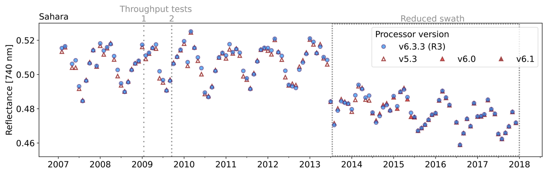
Figure 1 Monthly averaged reflectance measured by GOME-2A at 740 nm over the Sahara region (16–30° N, 8° W–29° E) as a function of time. Reflectances (R(λ)) are obtained by (πI(λ))/(I₀(λ)cos (θ₀)), where I(λ) is the radiance, I₀(λ) the solar irradiance and θ₀ the solar zenith angle. Reflectances obtained from the re-processed R3 level-1b data have processor version 6.3.3 and are shown in blue bullets. Reflectances of the previous level-1b dataset consist of different processor versions (v5.3, v6.0, and v6.1) and are shown in triangles with different hues of red. The reflectances from both level-1b datasets were co-sampled, and both data had to meet the criteria of cloud fraction <0.4. Data of days that are listed as outliers, including measurements in narrow swath, are excluded from both datasets. Events that impact the reflectance are indicated by dashed grey lines.

3 In-flight degradation correction

In this section, we describe a method to analyze and address the scan angle and wavelength dependency of degradation trends observed in the near-infrared GOME-2A reflectances. Adapted from the method used to correct for reflectance degradation in SCIAMACHY and GOME-2A for absorbing aerosol index (AAI) retrieval (Tilstra et al., 2012a, b), our in-flight degradation correction method examines daily global mean reflectance over time (t, per day), scan angle position (s), and wavelength (λ).

This more advanced approach improves upon the degradation correction used in SIFTER v2 (van Schaik et al., 2020), which relied on a wavelength-dependent seasonal factor with the 2007–2012 reflectance average as baseline. Furthermore, the correction was only applied to reflectances from June 2014 onward (see Table 2). In contrast, our method applies a continuous daily correction factor across the entire 2007–2017 record that addresses the early degradation patterns and the varying trends of degradation over time (e.g. before and after the throughput tests). Moreover, we include a scan angle dependency in the degradation correction. Findings from Tilstra et al. (2012b) and EUMETSAT (2022), which identified scan angle dependencies in GOME-2 reflectance – particularly in shorter wavelengths and in eastward-looking directions – prompted the inclusion.

We analyzed the global mean reflectances at each measured wavelength between 712 and 785 nm (in total 356 detector pixels), covering the SIF retrieval window (734–758 nm) and the spectral bands used to calculate the scene albedo (van Schaik et al., 2020). Valid reflectances of GOME-2A (R_λ,s) are collected between 60° S and 60° N, with solar zenith angles smaller than 85°, and averaged daily. Observations containing Sun glint or cloudy conditions are not filtered out, but days corresponding to narrow swath and nadir static measurements are excluded from the analysis. For GOME-2A, the scan position parameter s runs from 1 (eastward) to 24 (westward), considering only forward pixels. The daily global reflectance at 747.1 nm for the most eastward (s=1), center (s=12), and westward (s=24) pixels from 2007 to 2012 is shown in Fig. 2.

We modeled the variation in daily global mean reflectance ($R_{\mathit{\lambda },\mathrm{s}}^{*}$) using a Fourier series ($F_{\mathit{\lambda },\mathrm{s}}^q$), representing the seasonal variation, multiplied by a polynomial term ($P_{\mathit{\lambda },\mathrm{s}}^p$) to account for instrument degradation over time:

$$\begin{array}{}\text{(1)}& R_{\mathit{\lambda },\mathrm{s}}^{*}\left(t\right)=P_{\mathit{\lambda },\mathrm{s}}^p\left(t\right)[\mathrm{1}+F_{\mathit{\lambda },\mathrm{s}}^q(t\left)\right].\end{array}$$

Here, p denotes the degree of polynomial P_λ,s, and q represents the order of the finite Fourier series F_λ,s. P_λ,s is written as

$$\begin{array}{}\text{(2)}& P_{\mathit{\lambda },\mathrm{s}}^p\left(t\right)=\sum _{m=\mathrm{0}}^{\mathrm{p}}{u}_{\mathit{\lambda },\mathrm{s}}^m{t}^m,\end{array}$$

and $F_{\mathit{\lambda },\mathrm{s}}^q$ is defined as

$$\begin{array}{}\text{(3)}& F_{\mathit{\lambda },\mathrm{s}}^q\left(t\right)=\sum _{n=\mathrm{1}}^q\left[v_{\mathit{\lambda },\mathrm{s}}^n\cos \right(\mathrm{2}\mathit{\pi }nt)+w_{\mathit{\lambda },\mathrm{s}}^n\sin (\mathrm{2}\mathit{\pi }nt\left)\right].\end{array}$$

The implicit assumption is that the global averaged reflectance shows no long-term trends. Therefore, the observed trends captured by the polynomial are attributed to instrumental effects.

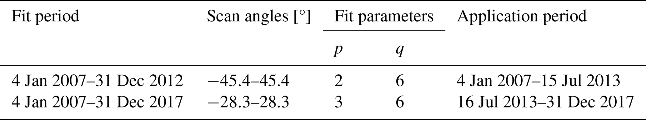
We analyzed $R_{\mathit{\lambda },\mathrm{s}}^{*}$ separately for the period before and after the reduced swath on 15 July 2013. Equation (1) is fitted to reflectances collected (i) between January 2007 and December 2012 and (ii) between January 2007 and December 2017. In the latter fit, reflectances between 2007 and 15 July 2013, were first interpolated to match the scan angles covered by the reduced swath. Each fit covers complete years to prevent biases from seasonal variation. Here, we set p=2 for the 2007–2012 fit and p=3 for the 2007–2017 fit. These higher-order polynomial degrees offer the flexibility to capture the varying behavior of the instrument degradation over time (discussed in Sect. 2). In both fits, q=6 was used for the order of the Fourier series. Table 1 summarizes the characteristics of the 2007–2012 and 2007–2017 fits. These fits are shown in Figs. 2 and S2, respectively.

The resulting 2007–2012 fits of $R_{\mathit{\lambda },\mathrm{s}}^{*}$ for the most eastern (s=1), center (s=12), and western (s=24) scan indices are shown as solid black lines in Fig. 2. These fits accurately follow the temporal pattern of the global reflectance, with correlations of 0.99, 0.99, and 0.98, respectively, for the scan indices 1, 12, and 24. The dashed lines represent the fitted polynomial component $P_{\mathit{\lambda },\mathrm{s}}^p$, illustrating the degradation effect over time. A gradually increasing trend is noted in the 747.1 nm reflectance, particularly at the most eastward position (s=1). This increase in reflectance results from the stronger decrease in measured solar irradiance (the denominator in R) than in measured radiance (the numerator in R). Furthermore, a slight reduction in increase is noted around 2010, possibly the result of the second throughput test in September 2009 (Fig. 1) (Munro et al., 2016; EUMETSAT, 2022).

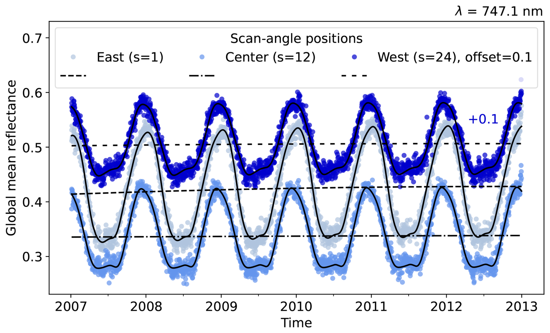
Figure 2 Global mean daily reflectance at 747.1 nm from GOME-2A over time, between 2007 and 2012, for the most eastward (s=0), center (s=12), and most westward (s=24) scan angle positions. Differences in magnitude and amplitude of the plotted reflectance time series are caused by the angular dependences of cloud and surface reflection. To separate the time series graphically, an offset of 0.1 was added only to the reflectances of the most westward scan angle position (s=24) (denoted in dark blue). The solid black lines show the fitted daily global reflectance $R_{\mathit{\lambda },\mathrm{s}}^{*}$, and the dashed black lines illustrate the effect of instrument degradation, as described in the main text.

Table 1 Summary of the characteristics for the fitted global mean reflectance over 2007–2012 and 2007–2017. Collected reflectances have latitudes between 60° S and 60° N and solar zenith angles <85°. The scan angles reflect the instrumental mirror angle, with ranges around −45.5–45.4° for the 1920 km swath and around −28.3–28.3° for the reduced 960 km swath (post-15 July 2013). Fitting parameters p an q represent the polynomial degree of P_λ,s and the order of the finite Fourier series F_λ,s in Eq. (1). The derived correction factors are applied to reflectances at 712–785 nm and scan index 1–24 to the specified application periods.

Finally, the correction for instrument degradation is obtained by scaling the polynomial value at each day to its value at the reference date (t₀):

$$\begin{array}{}\text{(4)}& c_{\mathit{\lambda },\mathrm{s}}\left(t\right)=P_{\mathit{\lambda },\mathrm{s}}^p\left(t_{\mathrm{0}}\right)/P_{\mathit{\lambda },\mathrm{s}}^p\left(t\right).\end{array}$$

The reference date for both fits, 2007–2012 and 2007–2017, is 5 January 2007. We use the polynomial from the 2007–2012 fit to derive the correction factors for January 2007 to mid-July 2013 and that of the 2007–2017 fit for mid-July 2013 to December 2017 (Table 1). We multiply these wavelength- and scan-angle-dependent corrections by the level-1b reflectances to correct for the degradation trends.

Figure 3 shows the averaged correction factor at 747.1 nm, broken down per year and scan angle, for the observations (a) before and (b) after the swath reduction. In both periods, the variation in correction factors across scan angle positions is of the same order as the variation over time, reaching up to 5 %. This indicates the significance of a scan-angle-dependent degradation correction. From 2007 to 2014 the annual averaged correction factors at 747.1 nm are below 1, meaning the reflectances were higher than the baseline in January 2007. From 2015, the correction factor for most scan indices exceeds 1 and then gradually increases further to correct for the decreasing reflectances over time.

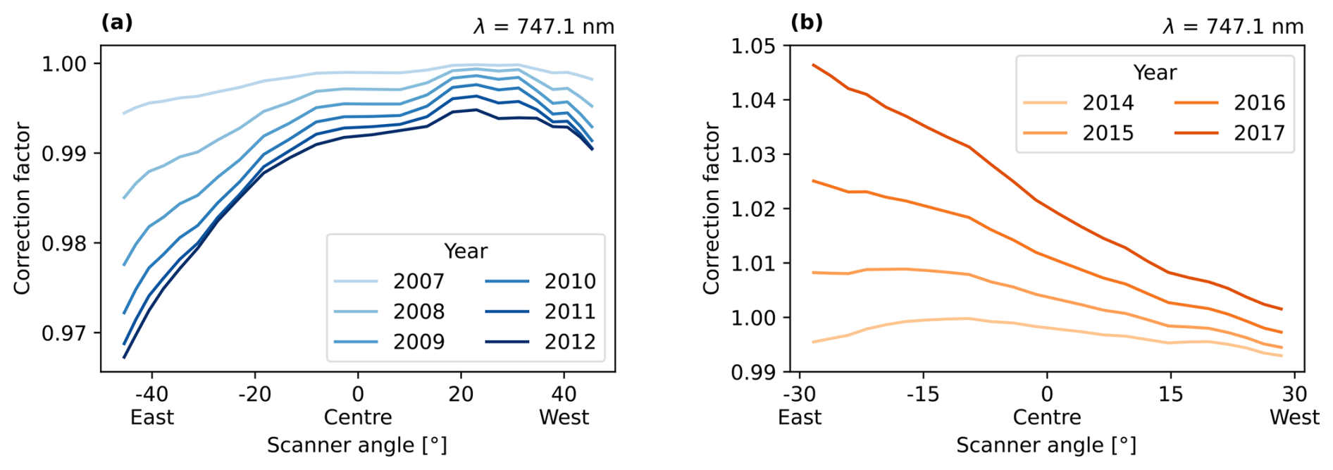
Figure 3 Reflectance degradation correction factors at wavelength 747.1 nm, averaged annually across the 24 scan angle positions. Panels (a) and (b) show the obtained corrections over the periods before and after the swath reduction on 15 July 2013, respectively. Only full-year averages are shown, so 2013 is omitted due to the mid-year swath reduction.

The gradual shifts in the correction factors over time are also visible in Fig. 4, which displays the factors over time and wavelength across the retrieval window range (734–758 nm) at a scan angle of −28.3° (s=1 for post-swath reduction period). The correction factors reflect the gradual increase of the reflectance from 2007, followed by a tipping point around 2011–2012 for most wavelengths, ultimately falling below the baseline of January 2007. This transition from lowering (c<1) to increasing corrections (c>1) occurs around 2014–2015, with this shift occurring earlier at shorter wavelengths.

Our analysis shows strong variations in reflectance over time, with increases around 2007–2012 followed by decreases from around 2014. These variations arise from the changing rates of throughput loss in both the Earth and solar paths, where the relative rates of throughput loss in these paths determine the observed fluctuations in reflectance. Overall, the impact of instrument degradation on the measured GOME-2 reflectance in the NIR shows a parabolic pattern with time, a stronger effect in the eastward scan positions, and a decrease with increasing wavelengths.

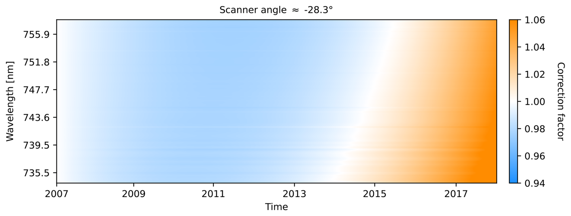
Figure 4 Temporal evolution of the degradation correction factors for each wavelength within the SIF retrieval window (734–758 nm, n=118) at a scan angle of −28.3°, representing the easternmost scan position, s=1, in the reduced-swath mode (similar to s=7 in the 1920 km swath). The shown correction factors are derived from the 2007–2017 reflectance fits.

4 SIFTER v3 retrieval algorithm

4.1 SIFTER retrieval algorithm

The SIFTER retrieval algorithm relies upon the relative infilling of solar Fraunhofer absorption lines in the radiance spectra by the far-red SIF (peak at ∼ 740 nm) – an approach pioneered by Joiner et al. (2011), Frankenberg et al. (2011b), and Guanter et al. (2012) for SIF retrieval from space. To detect the infilling of the narrow Fraunhofer lines from GOME-2A, with a spectral resolution of 0.5 nm, a spectral window covering multiple deep Fraunhofer lines is needed (Parazoo et al., 2019). From version 2 onwards, the SIFTER algorithm has used a relatively narrow retrieval window of 734–758 nm to limit complications by absorption signatures from water vapor and the O2-A band (van Schaik et al., 2020). The key of the retrieval is to separate the contributions of surface-emitted SIF from those of direct reflection to the overall reflectance. This is done by matching a modeled spectrum to the measured reflectance. Using a Lambertian model, the reflectance (R) can be written as

$$\begin{array}{}\text{(5)}& \begin{array}{rl}R(\mathit{\lambda },\mathit{\mu },{\mathit{\mu }}_{\mathrm{0}})& \approx a_{\mathrm{s}}\left(\mathit{\lambda }\right)T^{\downarrow }(\mathit{\lambda },{\mathit{\mu }}_{\mathrm{0}})T^{\uparrow }(\mathit{\lambda },\mathit{\mu })\\ & +{\displaystyle \frac{\mathit{\pi }{I}_{\mathrm{SIF}}\left(\mathit{\lambda }\right)}{E_{\mathrm{0}}\left(\mathit{\lambda }\right){\mathit{\mu }}_{\mathrm{0}}}}{T}^{\uparrow }(\mathit{\lambda },\mathit{\mu }),\end{array}\end{array}$$

where μ and μ₀ are the cosines of the viewing and solar zenith angles, respectively. The atmospheric molecular scattering in the near-infrared region is neglected (e.g. Joiner et al., 2013). In Eq. (5), a_s is the surface albedo; T^↑ and T^↓ are the upward and downwelling atmospheric transmission factors, respectively; I_SIF is the SIF emission at the Earth's vegetated surface; and E₀ is the solar irradiance. The SIFTER algorithm uses a fourth-order polynomial to describe the spectral surface albedo a_s. The atmospheric transmittance (T^↑, T^↓) is described by 10 principal components (PCs) that are obtained over non-vegetative areas.

The 10 basic functions describing the atmospheric transmittance are obtained in three main steps. First, a large ensemble of reflectance spectra without cloud coverage (cloud fraction <0.4) is collected over a non-vegetative reference area to represent the transmittance for a wide variety of conditions where I_SIF equals zero. The Sahara region (16–30° N, 8° W–29° E) is used as the reference area, and spectra are collected over the January 2007 to December 2012 period. Secondly, the contribution of the surface albedo to the spectra is eliminated by subtracting a second-order polynomial function obtained over spectral regions with negligible atmospheric absorption over no cloud conditions (described in more detail in van Schaik et al., 2020). Finally, using the widely used iterative principal component analysis NIPALS (nonlinear iterative partial least squares) (Esbensen et al., 2002), the first 10 principal component spectral functions (f_k(λ)) are retrieved that explain the variance within the spectra. Note that for the retrieval of data after the swath reduction in July 2013, PCs are obtained from spectra with viewing zenith angles <35° to match the observations in reduced swath.

Following the preparatory step of obtaining the 10 PCs, the SIFTER algorithm proceeds to fit a model to each individual reflectance spectrum by minimizing the differences between the observed and modeled reflectance spectra using a Levenberg–Marquardt least-squares regression (van Schaik et al., 2020). The modeled spectrum (R_m), follows on from Eq. (5) and is written as

$$\begin{array}{}\text{(6)}& \begin{array}{rl}{R}_{\mathrm{m}}(\mathit{\lambda },\mathit{\mu },{\mathit{\mu }}_{\mathrm{0}})& \approx \left(\sum _{j=\mathrm{1}}^n{a}_j{\mathit{\lambda }}^j\right)e^{-{\sum }_{k=\mathrm{1}}^m{b}_k{f}_k\left(\mathit{\lambda }\right)}\\ & +{\displaystyle \frac{\mathit{\pi }c{I}_{\mathrm{SIF}}\left(\mathit{\lambda }\right)}{{\mathit{\mu }}_{\mathrm{0}}\stackrel{\mathrm{‾}}{E_{\mathrm{0}}}}}{e}^{-\frac{{\mathit{\mu }}^{-\mathrm{1}}}{{\mathit{\mu }}^{-\mathrm{1}}+{\mathit{\mu }}_{\mathrm{0}}^{-\mathrm{1}}}{\sum }_{k=\mathrm{1}}^m{b}_k{f}_k\left(\mathit{\lambda }\right)}.\end{array}\end{array}$$

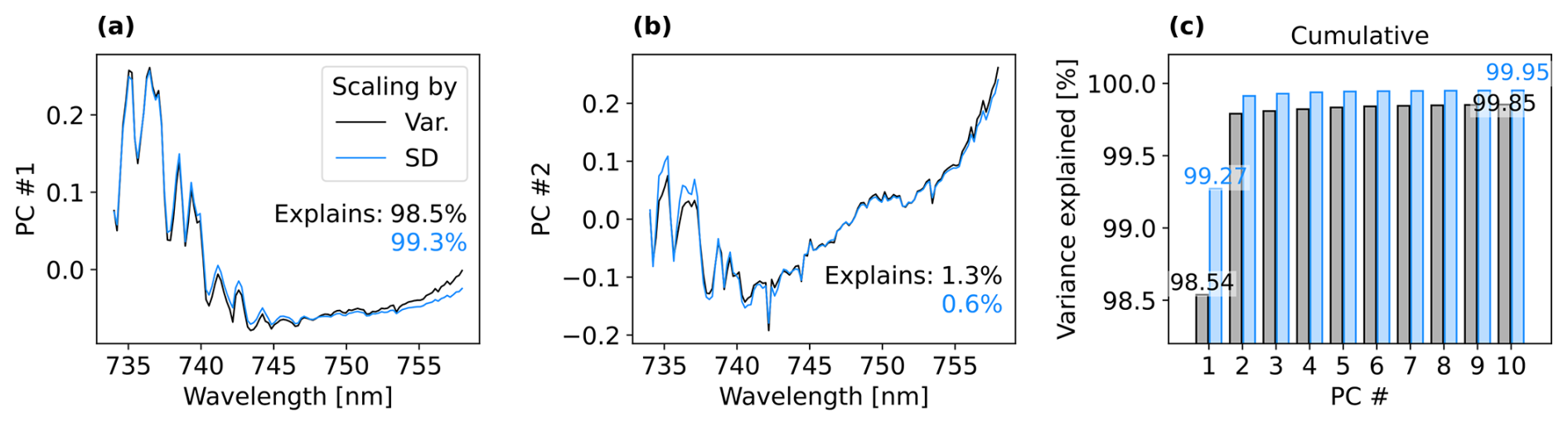
Figure 5 The leading principal components, (a) PC 1 and (b) PC 2, of GOME-2A reflectance spectra using scaling by the standard deviation (in black) and the variance (in blue) as a pre-treatment method prior to the principal component analysis. Panel (c) shows the cumulative explained variance of PCs 1 to 10 using both pre-treatment scaling methods. The PCs are obtained from collected GOME-2 reflectance spectra over the Sahara between 2007 and 2012.

Here a_j represents the fitting coefficients of the surface albedo, b_k is the coefficients that match the set of the 10 PCs, f_k(λ) describes the atmospheric transmission contribution to R, and c is the fit coefficient for I_SIF that characterizes the strength of the fluorescence signal. In total there are 16 fitting coefficients: 5 from a_j, 10 from b_k, and 1 from c. In Eq. (6), the solar irradiance, $\stackrel{\mathrm{‾}}{E_{\mathrm{0}}}$(λ), is taken to be the solar irradiance reference spectrum from Chance and Kurucz (2010), convolved with the GOME-2A slit function and scaled to the Earth–Sun distance. The solar irradiance reference spectrum is used in the model to mitigate the influence of instrument degradation on the observed solar irradiance (Sanders et al., 2016).

4.2 Processing and improvements of SIFTER v3 retrieval

The GOME-2A SIFTER v3 product presented here is an implementation of the general approach described in Sect. 4.1 and of three proposed revisions with respect to SIFTER v2, including the in-flight degradation correction described in Sect. 3. For the SIF retrieval process, EUMETSAT's reprocessed level-1b R3 data were used as input. The daily degradation correction factors were applied to stabilize the R3 reflectances over the entire 2007–2017 record. These degradation-corrected reflectances were then used to extract the 10 principal components (PCs) that describe the atmospheric transmission and to retrieve SIF. Figure S1 shows a flowchart of the processing algorithm. In this section we will discuss the proposed algorithm changes, listed in Table 2.

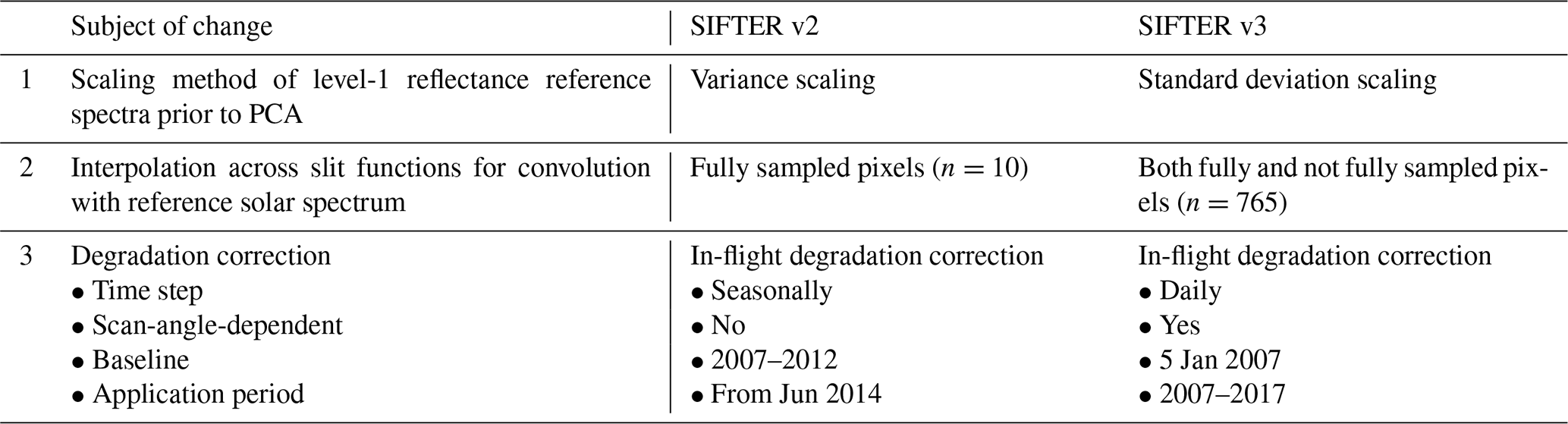
Table 2 Overview of the implemented changes, ordered by importance for the fit retrieval, in the SIFTER algorithm by this study: a comparison between SIFTER v3 and SIFTER v2 (van Schaik et al., 2020). The changes are placed in order of largest impact on the fit retrieval. Changes (1) and (2) are expected to significantly affect the fit quality of the retrieval, whereas alteration (3) is expected to mainly impact the consistency of SIF over time and across scan angles.

The first change concerns the pre-treatment of the reflectance reference spectra prior to the principal component analysis. In SIFTER v2, the collected level-1 reflectance spectra over the reference area (Sahara) underwent mean centering and scaling by the variance across wavelengths before conducting the principal component analysis (PCA). Our study explores an alternative “autoscaling method” that combines mean centering with scaling by the standard deviation, which ensures equal importance across the variables (van den Berg et al., 2006). Figure S4 demonstrates that the use of standard deviation scaling on the mean-centered spectra results in a more distinct pattern with tighter magnitude variations across the wavelengths as compared to variance scaling. This autoscaling approach outperforms the SIFTER v2 pretreatment method, with the 10 PCs explaining 99.95 % of the spectra variance compared to 99.85 %, as shown in Fig. 5c. More orthogonal PCs are expected to improve the fit by capturing the variation across wavelengths more consistently, leading to a more accurate representation of the atmospheric transmission.

Next, we discuss the revision of the convolution of the slit function with the solar irradiance reference spectrum. In the SIFTER algorithm, the high-resolution solar irradiance reference spectrum from Chance and Kurucz (2010) is used, convolved with the GOME-2A slit function and scaled to the Earth–Sun distance (Sanders et al., 2016; van Schaik et al., 2020). We denote this spectrum $\stackrel{\mathrm{‾}}{E_{\mathrm{0}}}$. Before this convolution can be done, we interpolate the slit functions across the wavelengths to match the high spectral resolution of the reference spectrum (Δλ=0.01 nm). We use slit functions in the range of ∼ 612–770 nm. In SIFTER v2, only the slit functions from fully sampled detector pixels (n=10) are used for the interpolation process, encompassing two spectral points within the retrieval window (Fig. S6). In this work, we include all slit functions provided in the key data (n=765), consisting both of fully sampled and not fully sampled pixels, which are interpolated by EUMETSAT as described in Siddans and Latter (2018). Figure S7a–d present the slit functions and their interpolation to the 0.01 nm spectral resolution, following the methods of SIFTER v3 and SIFTER v2, respectively.

Figure 6 shows the reference solar spectrum convolved with the slit functions as done in SIFTER v2 and in SIFTER v3 (this work). The solar irradiance spectrum convolved using the expanded slit function dataset follows the fine features of the Fraunhofer absorption lines better, resulting in deeper Fraunhofer lines than the convolved spectrum using only the fully sampled pixels. The solar irradiance reference spectrum $\stackrel{\mathrm{‾}}{E_{\mathrm{0}}}$ is applied at two instances in the algorithm retrieval. Firstly, the spectrum is used for high sampling interpolation of the measured solar irradiance spectrum to match the wavelength grid of the radiance measurements for the reflectance calculation. Secondly, the $\stackrel{\mathrm{‾}}{E_{\mathrm{0}}}$ spectrum is used in the modeled reflectance, Eq. (6), replacing the observed solar spectrum E₀, as discussed in Sect. 4.1.

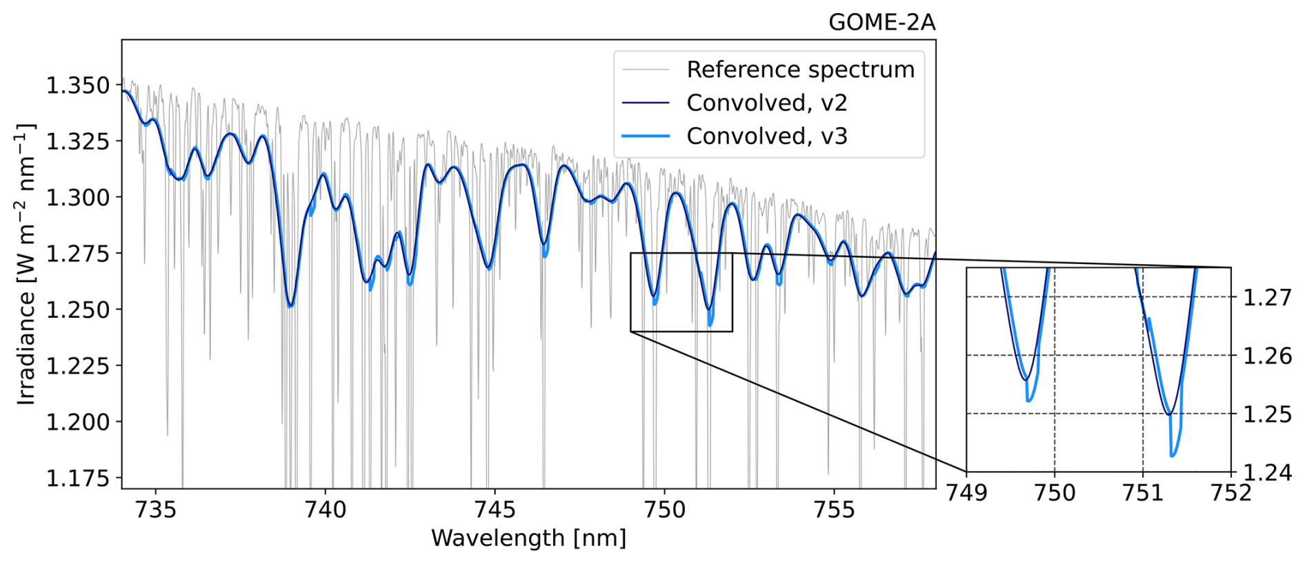
Figure 6 The solar irradiance reference spectrum of Chance and Kurucz (2010) convolved with the GOME-2A slit function (in grey) and the Chance and Kurucz (2010) spectrum convolved with the interpolated SIFTER v2 slit function (using fully sampled pixels) (in black) and the interpolated SIFTER v3 slit function (using fully and not-fully sampled pixels) (in blue).

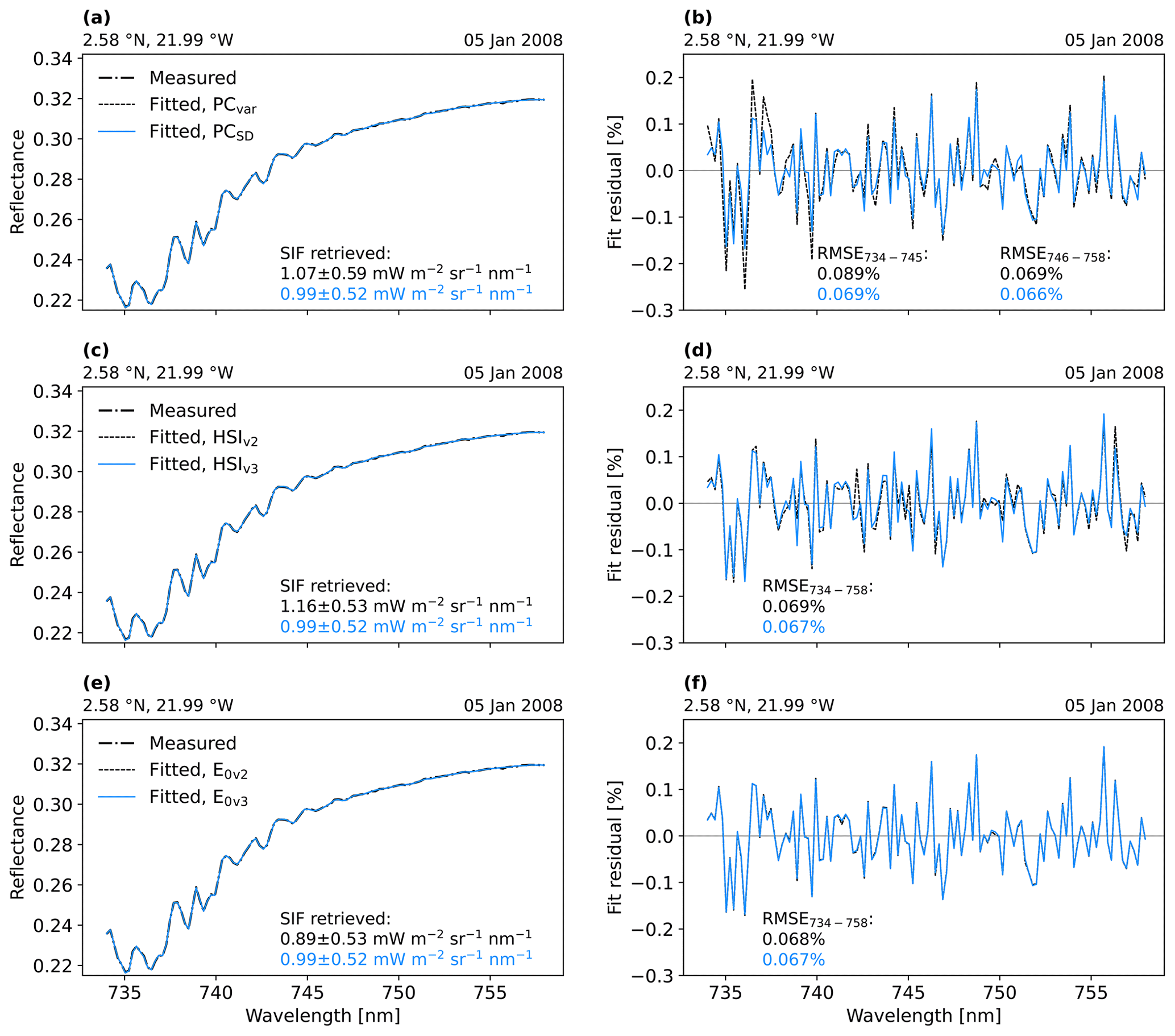
Figure 7 SIF retrieval from GOME-2A of a single pixel over the Congo Basin (2.58° N, 21.99° W) on 5 January 2008. The left panels show the observed reflectance and fitted reflectances, and the right panels show the fit's residuals. Plots (a) and (b) show the fitted reflectance and its residuals using PCs computed with standard deviation and variance as pretreatment scaling factors, respectively referred to as PC_SD and PC_var. Plots (c) and (d) show the fitted reflectance and its residuals for retrievals from reflectances obtained using the SIFTER v3 and SIFTER v2 wavelength calibration, referred to as HSI_v3 and HSI_v2, respectively. Plots (e) and (f) show the fitted reflectance and the fit residuals from retrievals using reference spectra convolved with slit functions interpolated according to SIFTER v3 and SIFTER v2 as the solar irradiance E₀, referred to as E_0,v3 and E_0,v2, respectively. The stated SIF values reflect the values from the retrieval step and are not corrected for the latitude bias.

To understand the impact of each individual algorithm change, we examine the impact on the retrieved SIF and its fit residuals. Here, the two usages of the changed solar irradiance reference spectrum are seen as two individual changes. Figure 7 shows the spectral fit (on the left) and fit residuals (on the right) over a single Congo Basin pixel using the SIFTER v3 algorithm (depicted in blue) and algorithm settings where one of the subjects of change is set to SIFTER v2 (depicted in dashed black lines). The difference between both fits illustrates the impact of the specific change made in SIFTER v3.

Figure 7a shows the spectral fit over a single Congo Basin pixel with PCs obtained when using (i) the variance as scaling factor as in SIFTER v2 and (ii) the standard deviation as a scaling factor. The use of the standard deviation scaling factor results in lower SIF (0.99 mW m⁻² sr⁻¹ nm⁻¹), compared to the variance scaling factor (1.07 mW⁻² sr⁻¹ nm⁻¹). Furthermore, PC_SD resulted in more homogenized and lower fit residual across the spectrum, as seen by the RMSE (Fig. 7b). Notably, PC_var had more difficulty to explain the 734–745 nm region of the spectrum (RMSE of 0.089 %), where water absorption features are more prominent, in comparison to the PC_SD (RMSE of 0.069 %) over the same spectral region. The observation of reduced fit residuals when PC_SD is used, specifically over 734–745 nm, holds true across a larger ensemble of pixels (Congo Basin, n=644), as illustrated in Fig. S5. This confirms that the proposed autoscaling pretreatment method results in PCs that better describe the atmospheric transmission (including the water vapor absorption), resulting in a better fit of the retrievals.

Figure 7c presents the fitted reflectance and the fit residual on the single Congo Basin pixel for retrievals with input reflectances that use high sampling interpolation obtained from the solar irradiance reference spectrum $\stackrel{\mathrm{‾}}{E_{\mathrm{0}}}$ as (i) in SIFTER v2 (HSI_v2) and (ii) in SIFTER v3 (HSI_v3). The HSI_v3 reflectances resulted in a reduction in SIF by 15 % in comparison to the HSI_v2. Additionally, employing all key data did result in a slightly better fit as seen from the reduction in fit residuals (Fig. 7d). This showcases the strong sensitivity of the SIF retrieval algorithm to slight changes in the reflectances.

Figure 7e shows the fit results and residuals for the use of $\stackrel{\mathrm{‾}}{E_{\mathrm{0}}}$ as obtained in SIFTER v2, $\stackrel{\mathrm{‾}}{E_{\mathrm{0},\mathrm{v}\mathrm{2}}}$, and SIFTER v3, $\stackrel{\mathrm{‾}}{E_{\mathrm{0},\mathrm{v}\mathrm{3}}}$ on the single Congo Basin pixel. The retrieved SIF slightly increased from 0.89 to 0.99 mW m⁻² sr⁻¹ nm⁻¹ when $\stackrel{\mathrm{‾}}{E_{\mathrm{0},\mathrm{v}\mathrm{3}}}$ is used instead of $\stackrel{\mathrm{‾}}{E_{\mathrm{0},\mathrm{v}\mathrm{2}}}$ in the modeled reflectance. This increase results from the deeper Fraunhofer absorption lines in the solar irradiance reference spectrum convolved with the slit function obtained using the SIFTER v3 method (see Fig. 6).

Finally, to study the effects of the algorithm revisions on the retrieval performance in tandem, and for a larger ensemble of pixels, we conducted a series of four experiments in which the revisions are progressively introduced from SIFTER v2 to SIFTER v3 methodology. The first experiment is based on the SIFTER v3 algorithm approach but with the use of (i) the variance scaling pre-treatment method (PC_var) and the solar irradiance reference spectrum convolved with GOME-2A slit function as done in SIFTER v2 ($\stackrel{\mathrm{‾}}{{\mathrm{E}}_{\mathrm{0},\mathrm{v}\mathrm{2}}}$) for (ii) the high sampling interpolation (HSI_v2) and (iii) computation of the modeled reflectance. The last experiment implements all revisions proposed in this work. Table 3 shows the results of the experiments over 678 pixels on 5 January 2008, over the Congo Basin (13° S–6° N, 14–31° W).

Table 3 Summary of experiment results on the progressive revisions from SIFTER v2 (experiment 1) to SIFTER v3 (experiment 4) settings over 678 pixels in the Congo Basin (13° S–6° N, 14–31° W) on 5 January 2008. The selected pixels of the four experiments were co-sampled and had to meet the requirements of autocorrelation <0.2 and cloud fraction <0.4. The scan-angle-dependent degradation correction as implemented in SIFTER v3 was used in all experiments.

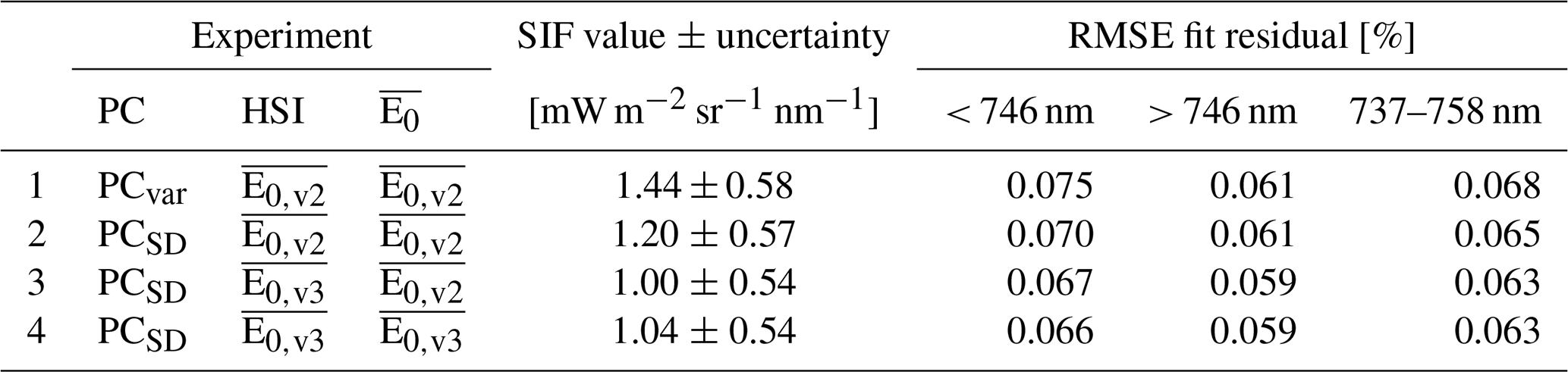
The revision of the pre-treatment scaling method before the principal component had the most substantial impact on both the magnitude of SIF and the retrieval fit. The use of the $\stackrel{\mathrm{‾}}{{\mathrm{E}}_{\mathrm{0},\mathrm{v}\mathrm{3}}}$ showed the largest effect in terms of altering the reflectance in its use for the wavelength calibration of the irradiance observations to match the radiance wavelength grid. The results indicate that the discussed revisions in SIFTER v3 decreased the magnitude of SIF by 28 %, from 1.44 to 1.04 mW m⁻² sr⁻¹ nm⁻¹, but substantially improved the retrieval fit quality from 0.068 % to 0.063 % RMSE fit residuals. The proposed revisions decrease the sensitivity to water vapor, as indicated by the reduced RMSE fit residual over the 734–746 nm where water vapor features are present. This improvement is mainly attributed to the autoscaling method in the pre-treatment of the principal component analysis, resulting in PCs that better capture the water vapor features.

4.3 Zero-level offset adjustment

Our retrieval detects the presence of chlorophyll fluorescence as changes in the relative depth of the Fraunhofer lines. However, instrumental effects and artifacts can also cause infilling, or deepening, of the Fraunhofer lines, making it indistinguishable from true fluorescence signals (e.g. Frankenberg et al., 2011a; Joiner et al., 2012; Khosravi et al., 2015). These false SIF signals are denoted as so-called zero-level offsets over vegetation-free regions and may be of the same order of magnitude as SIF (Köhler et al., 2015). Previous studies have found a particularly strong latitude dependency in GOME-2A SIF over oceans (e.g. Köhler et al., 2015; Joiner et al., 2016; van Schaik et al., 2020). This latitudinal bias is possibly related to the varying width of the slit function, driven by the changing temperatures of the instrument in the descending orbit (Munro et al., 2016). Specifically, the widening of the slit function, due to a higher optical bench temperature, may cause ever shallower Fraunhofer lines along the orbit, which the SIFTER algorithm would interpret as infilling by chlorophyll fluorescence, while a narrower slit function results in deeper Fraunhofer lines, leading to retrieved negative SIF values over unvegetated regions.

Such a zero-level offset is indeed visible in the new SIFTER v3 data. The effect in SIF is visualized in Fig. 8a (blue line), showing a negative trend over the Northern Hemisphere and a positive trend over the Southern Hemisphere above the Pacific Ocean, where SIF is expected to equal zero. Here we apply a post hoc correction to adjust for the observed bias. The applied adjustment was adapted from the method of SIFTER v2. In this method, van Schaik et al. (2020) obtained day- and latitude-band-specific regression coefficients between collected reflectance (at 744 nm) and SIF data per 1° latitude band over the Pacific Ocean (130–150° W). Data were collected from up to 14 d back if the minimum number of 10 points per 1° latitude band was not met. These regression coefficients, slope a and offset b, were used to get the bias (B_lat) for each pixel, at day t and within latitude band lat, based on its reflectance at 744 nm (R), as shown in Eq. (7).

$$\begin{array}{}\text{(7)}& B_{t,\text{lat}}=a_{t,\mathrm{lat}}\cdot R\left({\mathit{\lambda }}_{\mathrm{744}}\right)+b_{t,\mathrm{lat}}\end{array}$$

Since the bias is additive due to the false infilling or false deepening, SIF is adjusted for the bias by subtracting the estimated bias; see Eq. (8).

$$\begin{array}{}\text{(8)}& {I^{\prime }}_{\text{SIF}}=I_{\mathrm{SIF}}-B_{t,\text{lat}}\end{array}$$

Here we made two modifications from the adjustment method of SIFTER v2. First, we extended the non-vegetative area to obtain the regression coefficients from to cover a broader latitude range. Not only the Pacific Ocean (130–150° W) but also a box over Atlantic Ocean (12° W–2° E) are used as the reference area. Secondly, we relaxed the filtering criteria to include pixels with any cloud fraction to calculate the regression coefficients, instead of the <0.4 requirement as used in van Schaik et al. (2020). Accepting pixels over the reference area with any cloud fraction does not only significantly enhance the number of collected pixels, which resulted in better fits, but also enables representation of pixels with higher radiance values. Representativeness of higher radiance values is hypothesized to help address biases over non-vegetative desert area (Joiner et al., 2016).

The light-blue line in Fig. 8a represents SIF with the post hoc bias adjustment, gridded per latitude band. The adjusted SIF portrays a realistic near zero-line across latitude over the Pacific ocean, indicating that the adjustment methods succeeds in removing the latitude-dependent bias. The effect of the adjustment is also noted when comparing unadjusted (Fig. 8a) and adjusted SIF (Fig. 8b). The adjusted SIF shows values around zero over the oceans, and adjusted SIF no longer suffers from negative values over the desert areas.

Next, to evaluate the impact of the inclusion of cloudy pixels in constructing latitude bias adjustment in Eq. (7), we constructed the latitude bias correction using SIFTER v3 SIF with cloud fraction requirements, as in SIFTER v2. Figure S8 shows that the resulting latitude bias is more negative over the Sahara area as compared to no cloud filtering. This more negative bias correction can lead to unrealistic SIF values exceeding well over zero. It indicates that including cloudy pixels in the latitude bias computation indeed provides more accurate adjusted SIF values, particularly over desert areas.

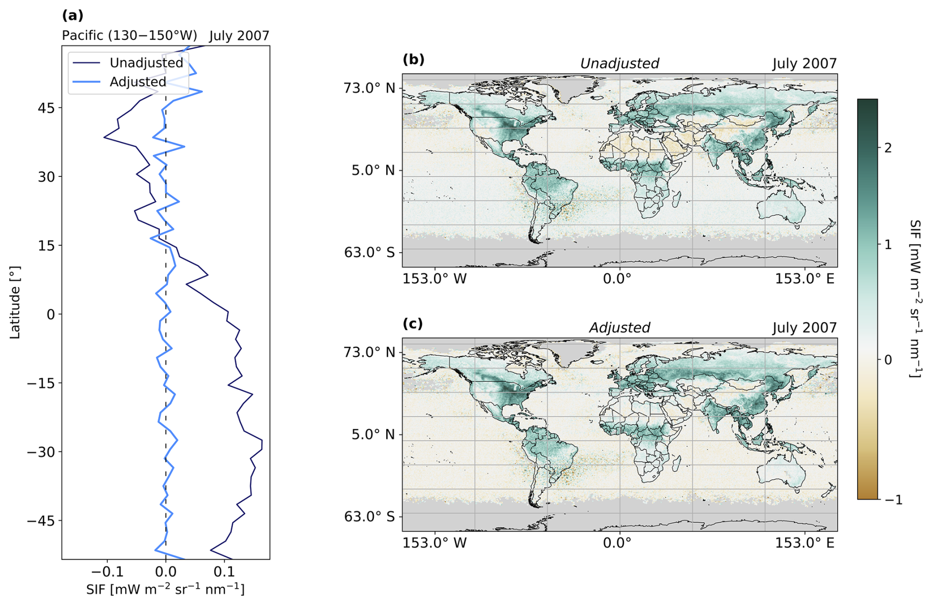
Figure 8 (a) Adjusted (light-blue line) and unadjusted (thin dark-blue line) instantaneous SIF over the Pacific Ocean averaged per latitude band of 2° and over July 2007, (b) level-2 SIF averaged over July 2007 without zero-level offset correction, and (c) level-2 SIF averaged over July 2007 with zero-level offset correction as post hoc correction.

5 SIFTER v3 retrieval results

5.1 Impact of in-flight degradation correction on retrieved SIF

To examine the impact of our degradation correction on the SIF retrievals, we compared time series of SIFTER v3 SIF values retrieved from corrected and uncorrected reflectances. Both SIF values, degradation corrected and uncorrected, were adjusted for the zero-level bias. Figure 9 shows this comparison across the Sahara (unvegetated) and five diverse vegetated areas: eastern Europe, the United States Corn Belt, the Amazon, the Congo Basin, and southeastern Australia.

In eastern Europe, the United States Corn Belt, the Amazon, and the Congo Basin, uncorrected SIF values (thin dark-blue line) surpass degradation-corrected SIF values (light-blue line) before 2014. After 2014, uncorrected SIF falls below the corrected values. For instance, in 2010, the average degradation-corrected SIF over the United States Corn Belt was 0.67 mW m⁻² sr⁻¹ nm⁻¹, while the uncorrected SIF averaged 0.71 mW m⁻² sr⁻¹ nm⁻¹, representing a 2.8 % difference. By 2016, the corrected SIF values were 5.6 % higher than the uncorrected SIF in the same region. The largest difference between the degradation-corrected and uncorrected SIF is found over the Amazon region between 2014–2017, with a discrepancy of +11.1 %. The observed patterns indicate that degradation correction reduces SIF values in the earlier years and increases them in later years, reflecting the inverse function of the applied degradation factors. In the absence of an appropriate degradation correction, deviations from true reflectance values are, at least partly, being misattributed as SIF values by the retrieval algorithm.

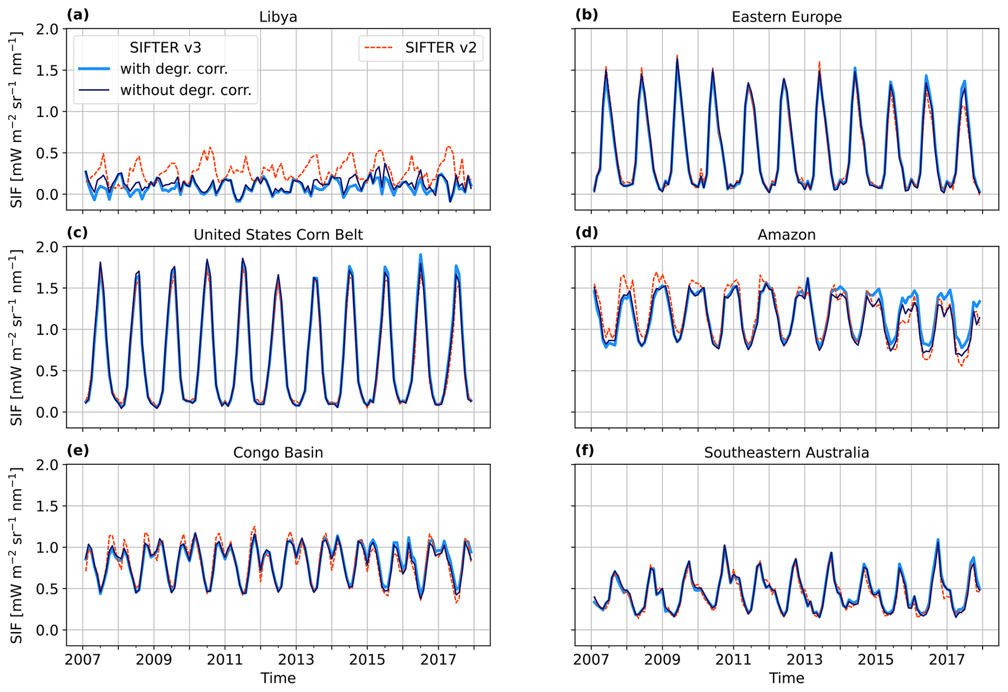
Figure 9 Time series of level-2 instantaneous SIF retrieved with the SIFTER v3 algorithm with (solid light-blue line) and without the in-flight degradation correction (thin dark-blue line) over the Sahara (16–30° N, 8° W–29° E) and vegetated areas: eastern Europe (50–55° N, 24–39° E), the United States Corn Belt (38–46° N, 81–96° W), Amazon (0–15° S, 55–70° W), Congo Basin (13° S–6° N, 14–31° E), and southeastern Australia (35.5–38° S, 141.5–149.5° E). Co-sampled SIF data from SIFTER v2 are plotted in a dashed orange line.

The zero-level offset adjustment, included in the time series shown in Fig. 9, could impact the consistency of SIF over time. To isolate the effect of degradation correction from this post hoc correction, we compared the time series of SIFTER v3 with and without the degradation correction for both adjusted (final product) and unadjusted values in eastern Europe and the United States Corn Belt, as shown in Fig.  S11. We observed a clear decreasing trend in annual maximum SIF values in the uncorrected SIF values when the zero-level offset adjustment is not applied, but this trend disappears when the adjustment is applied. This suggests that the post hoc correction plays a significant role in removing the degradation trend in the uncorrected SIF. This diminishing effect of the post hoc correction is further emphasized by a 5.6 % and 23.3 % difference in degradation-corrected versus uncorrected SIF over the United States Corn Belt in 2016, respectively with and without the post hoc zero-level offset adjustment.

Overall, the degradation correction effectively removes spurious trends over time, resulting in more consistent SIF time series. The full impact of our algorithm revisions on the SIF product will be assessed by comparing SIFTER v3 with the previous dataset, SIFTER v2, in Sect. 5.2.

5.2 Comparison of SIFTER v3 with SIFTER v2

We compared SIF from the new SIFTER v3 with our previous product, SIFTER v2 (van Schaik et al., 2020). We co-sampled the datasets to allow a fair comparison. The re-processed level-1b R3 dataset used in v3 includes a different version of FRESCO+, resulting in slight changes in effective cloud fractions compared to the previous v2 (Fig. S9S). Figure 9 illustrates the time series for both SIFTER products across unvegetated Sahara area and five vegetated areas. The analysis over the Sahara, where SIF is expected to remain near zero, serves as a validity check. The new product reflects this validity, with an average of 0.08±0.08 mW m⁻² sr⁻¹ nm⁻¹, while the previous product fluctuates around 0.27± 0.13 mW m⁻² sr⁻¹ nm⁻¹. This discrepancy may be attributed to the revision in the zero-level offset adjustment calculation, as discussed in Sect. 4.3.

Clear seasonal patterns are observed in both products across the vegetative regions. In eastern Europe, the Amazon, and the Congo Basin, SIFTER v2 shows higher values than SIFTER v3 until around 2013, after which it drops below SIFTER v3. For example, in 2010, v2 shows values of 1.32 mW m⁻² sr⁻¹ nm⁻¹ over the Amazon, compared to 1.21 mW m⁻² sr⁻¹ nm⁻¹ from v3 – an 8.2 % difference. By 2016, the v2 annual average is 11.3 % lower than that of the new v3 product. This pattern aligns with trends in reflectance degradation before 2014 (see Fig. 2). A similar trend was found when comparing degradation-corrected SIFTER v3 with the uncorrected values, as discussed in Sect. 5.1.

Table 4 shows SIFTER v3 and SIFTER v3 values for January and July 2008 across the vegetated areas. The year 2008 was chosen to minimize degradation-related differences. The magnitudes in SIF are similar, with a maximum difference of around −10 % over the Amazon in January. The higher SIFTER v2 values were expected following the algorithm revisions (see Table 3). For the analyzed vegetated regions and months, v3 exhibits lower standard deviation and variability than v2. This suggests improved precision and consistency of SIFTER v3. This is supported by the lower uncertainty in the SIFTER v3 SIF values, which is approximately 13 % lower on 8 January 2008, as shown in Fig. 10. The lower uncertainty of SIFTER v3, around 10 %, in comparison to SIFTER v2, remains consistent in later periods when instrument degradation led to a decrease in measurement accuracy (Fig. 10). These increased precisions result from reduced fit residuals following the revisions in the SIFTER algorithm (Table 3).

Overall, SIFTER v3 demonstrates enhanced consistency over space and time and precision compared to SIFTER v2. However, to confirm whether the new version accurately captures the interannual variation of vegetation activity across the 2007–2017 record, further evaluation against independent data is necessary. This will be further analyzed and discussed in Sect. 5.3.

Table 4 Monthly mean of co-sampled instantaneous SIF values from SIFTER v3 and SIFTER v2 for the different vegetated regions as shown in Fig. 9 for January and July 2008. The uncertainties reflect the standard deviation. SIFTER data have been selected for autocorrelation values <0.2 and cloud fraction <0.4.

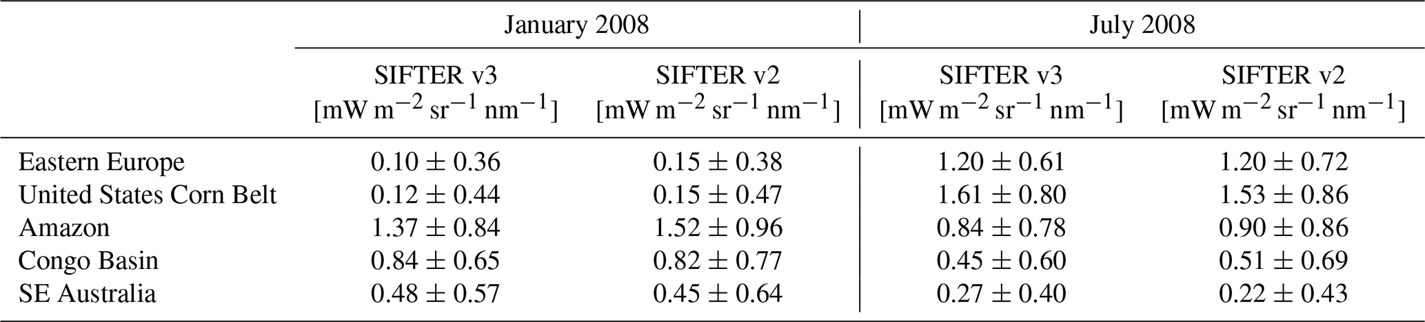
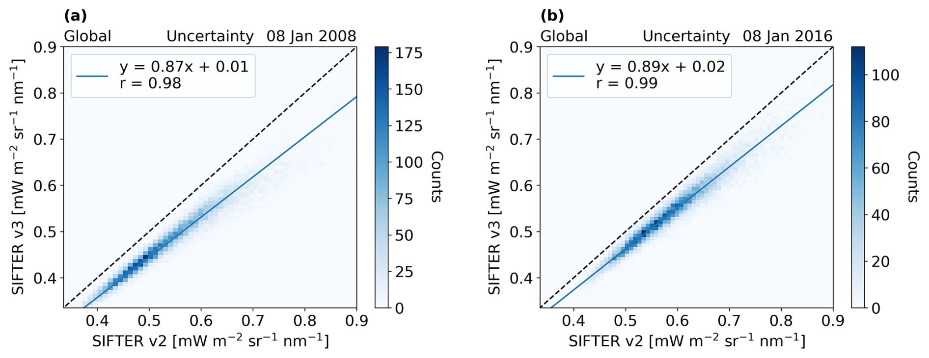
Figure 10 Pixel-by-pixel comparison of the uncertainty of SIFTER v3 and SIFTER v2 derived over all land pixels on (a) 8 January 2008 and on (b) 1 July 2008. The pixels cover the global land area and are filtered for autocorrelation values <0.2 and cloud fractions <0.4.

5.3 Evaluation of SIFTER v3 with independent SIF and GPP observations

To evaluate the ability of SIFTER v3 to accurately track vegetation activity over time, we compared it with the latest version of NASA GOME-2A SIF (Joiner et al., 2023), as well as two independent datasets, namely FluxSat GPP (Joiner et al., 2018) and FLUXCOM-X (Nelson et al., 2024). Both state-of-art GPP products are widely used to track interannual variations in GPP, are known for capturing drought events (Byrne et al., 2021; Chen et al., 2021; Lv et al., 2023), and align well with GPP estimates from independent flux towers (Joiner et al., 2018; Zhang et al., 2023).

The NASA SIF product retrieved from GOME-2A uses the same retrieval window (734–758 nm) as SIFTER v3 and applies a similar PCA-based approach to model atmospheric transmittance (Joiner et al., 2013, 2016). The main differences between NASA SIF and SIFTER v3 lie in the absence of degradation correction and the use of a machine learning approach to address the zero-level offset (Joiner et al., 2020).

FluxSat GPP is a high-resolution, 0.05° × 0.05°, satellite-derived dataset obtained using a neural network approach and daily-scaled MODIS reflectance (MCD43) data to upscale GPP estimates from eddy-covariance flux towers (FLUXNET 2015). FLUXCOM-X similarly upscales GPP estimates from eddy-covariance data and daily-scaled MODIS reflectance data but also incorporates meteorological data from the ERA5 reanalysis products, land surface temperature observations, and land cover information (Tramontana et al., 2016; Jung et al., 2019; Nelson et al., 2024). The variations in FLUXCOM-X are driven by MODIS remote sensing data (Nelson et al., 2024). This product is obtained through a machine learning approach based on gradient boosted regression trees implemented with the XGBoost library, and it has a hourly temporal scale with a spatial resolution of 0.05° × 0.05° (Nelson et al., 2024).

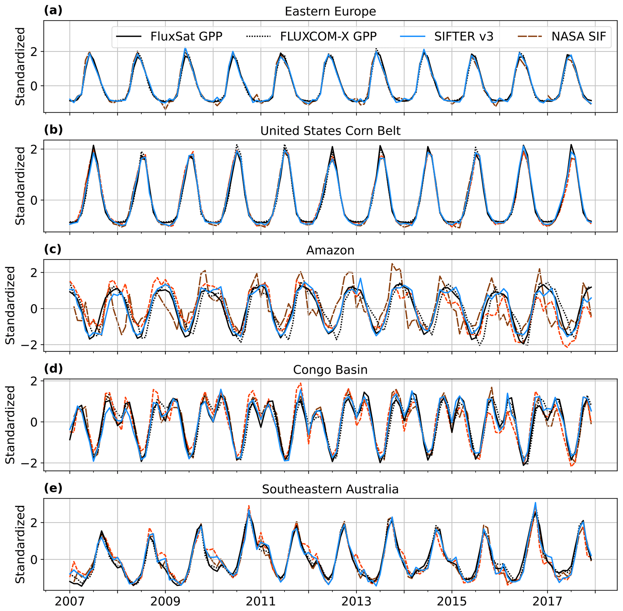
Figure 11 Time series of standardized FluxSat GPP (solid black line), FLUXCOM-X GPP (dashed black line), and SIF from SIFTER v3 (solid blue line), SIFTER v2 (dashed orange line), and NASA SIF (dashed brown line) across the five vegetative regions of Fig. 9. GOME-2A SIF data from SIFTER v3, SIFTER v2, and the NASA product were filtered for cloud fractions <0.4. All data are monthly averaged. The monthly data are standardized by subtracting each value (x) by the averaged value over all months (μ), divided by the standard deviation across 2007–2017 (σ); the standardized value is calculated as $x=(x_{\mathrm{0}}-\mathit{\mu })/\mathit{\sigma }$.

Figure 11 shows standardized monthly averaged time series FluxSat GPP, FLUXCOM-X GPP, SIFTER v3, SIFTER v2, and NASA SIF for the vegetative regions shown in Fig. 9 and Table 4. The standardization adjusts the dataset in a way that the values are expressed in units of standard deviation from the mean (also see the caption of Fig. 11). This adjustment allows for direct comparison of the SIF and GPP products at the same scale. The seasonal patterns of FluxSat GPP compared well with both SIFTER products, indicating that SIFTER effectively captures the seasonal variability across different geographical regions. FLUXCOM-X GPP also closely follows both SIFTER products and FluxSat GPP, although deviations are observed in the Amazon and Congo Basin regions, which may result from known challenges in capturing carbon fluxes over the tropics (Tramontana et al., 2016).

NASA SIF captures the seasonality observed in both SIFTER and GPP products across most regions, though significant discrepancies are noted over the Amazon. A lower correlation between SIF and GPP in the Amazon compared to other regions is also observed for SIFTER v3. However, strong correlations, such as r=0.95 with FluxSat (Fig. S15) and r=0.85 with FLUXCOM-X (Fig. S16), suggest the ability of SIFTER v3 to track the seasonality in this region. In contrast, weaker correlations between NASA SIF and FluxSat GPP (r=0.40) and FLUXCOM-X GPP (r=0.13), suggest difficulty for NASA SIF in capturing the seasonal dynamics of the Amazon (Fig. S17). Across other regions, NASA SIF and SIFTER v3 show strong agreement, with correlations as high as r=0.99 over eastern Europe (Fig. S18). Furthermore, SIFTER v3 consistently shows stronger correlations with both FluxSat and FLUXCOM-X GPP than NASA SIF.

SIFTER v3 follows the seasonal peaks and troughs depicted by FluxSat GPP more accurately, compared to SIFTER v2. This is particularly evident in the Amazon region where SIFTER v2 shows a decreasing trend between 2014 and 2017, while SIFTER v3 and FluxSat GPP remains more consistent over time. We found a consistent pattern of overestimation (before 2014) and underestimation (after 2014) by SIFTER v2 relative to FluxSat GPP. This pattern, also observed in Fig. 9 and discussed in Sect. 5.1 and 5.2, emphasizes that the lack of degradation correction in SIFTER v2 from 2007 to 2013 led to an overestimation of SIF and that the applied correction in the later years did not remove degradation effects completely.

Overall, SIFTER v3 highly correlates with FluxSat GPP (r=0.91–0.99, Fig. S15) and FLUXCOM-X GPP (r=0.85–0.99, Fig. S16) across all regions, indicating strong consistency, both temporally and spatially, in capturing vegetation activity over the record. Compared to SIFTER v2, SIFTER v3 shows higher correlation with both GPP products, reflecting a more robust and consistent pattern interannual variations in SIF over the 2007–2017 period. Moreover, SIFTER v3 data exhibits a significantly reduced spread in values, with measurements more tightly clustered together compared to SIFTER v2. This reduced variability indicates that the improvements in the SIFTER v3 algorithm have successfully minimized outliers, leading to enhanced consistency and precision in the SIF dataset.

6 Conclusions

We improved the Solar-Induced Fluorescence of Terrestrial Ecosystems Retrieval (SIFTER) retrieval algorithm to obtain a more consistent and accurate solar-induced fluorescence (SIF) long-term record SIF record from the GOME-2A instrument for 2007–2017. Although GOME-2A data extend to 2021, measurements beyond 2018 were excluded due to orbital control issues of Metop-A. The updated algorithm, SIFTER v3, uses the recalibrated and reprocessed GOME-2A level-1b Release 3 (R3) data as input. Additionally, it incorporates an enhanced understanding of the instrument's characteristics, leading to strong improvements in fit uncertainty, and spatial and temporal consistency.

We found that the level-1b R3 data are more consistent than previous level-1 version, but instrument degradation still affects the reflectance data. We found that the reflectance degradation strongly depends on time, wavelength, and scan angle. The reflection degradation manifests already early in the record and evolves over time, in response to throughput tests, and different trends in radiance and irradiance degradation. To address these degradation-related trends, our SIFTER v3 algorithm applies a correction that depends on time (daily time step), wavelength, and scan angle, on the observed R3 reflectances. Compared to SIFTER v2, which only corrected for degradation from June 2014 and lacked scan angle dependency, SIFTER v3 provides more consistent SIF records.

Other improvements made to the SIFTER algorithm include more orthogonal principal components (PCs) and a better representation of slit function variation across spectra. The latter resulted in more realistic solar irradiance $\stackrel{\mathrm{‾}}{E_{\mathrm{0}}\left(\mathit{\lambda }\right)}$ with deeper Fraunhofer lines. These algorithm revisions led to lower magnitudes in SIF and reduced fit residuals across the retrieval window. Particularly, the new PCs improved the performance over the 734–745 nm region, where water vapor features are present, leading to a ∼14 % reduction in fit residuals. In SIFTER v3, the uncertainty in retrieved SIF decreased by approximately 10 % compared to SIFTER v2, which is the direct result of the reduced fit residuals. The improved temporal consistency of SIFTER v3 is most evident in tropical regions with higher atmospheric water vapor content, like the Amazon and the Congo Basin, highlighting its enhanced ability to capture the atmospheric effects on the spectra, particularly the effect of water vapor absorption.

Despite these improvements, a persistent latitude bias remained, observed as a zero-level offset over non-vegetative areas. This zero-level offset bias is most likely due to varying slit functions in response to instrumental temperature warming across the orbit. To correct for this, we derived daily latitude-dependent adjustments over the Pacific and Atlantic Oceans. These adjustments are applied as a post hoc correction (additive). SIFTER v3 obtains the adjustments from all pixels – both cloudy and clear-sky – while SIFTER v2 solely used clear-sky pixels. Including cloudy pixels to obtain the zero-level adjustment enhanced the adjustment's representativeness in desert deserts. As a result, SIFTER v3 shows more realistic values of 0.08 mW m⁻² sr⁻¹ nm⁻¹ over the Sahara area, compared to SIFTER v2, with less realistic SIF values of 0.27 mW m⁻² sr⁻¹ nm⁻¹.

We evaluated the new data record against NASA GOME-2A SIF and independent FluxSat GPP data and FLUXCOM-X GPP data. SIFTER v3 is strongly correlated with FluxSat GPP across different biomes and outperforms SIFTER v2. This improved performance is also observed when comparing FLUXCOM-X GPP with the new and previous SIFTER product. Throughout the entire 2007–2017 period, SIFTER v3 showed strong temporal consistency with both GPP products, without signs of degradation-induced false trends. Additionally, SIFTER v3 exhibited substantially reduced variability across all analyzed regions. Furthermore, SIFTER v3 shows strong correlations with NASA SIF, except over the Amazon region, likely due to challenges faced by NASA SIF in capturing the seasonal dynamics in this region.

In conclusion, our new SIFTER v3 product resulted in more robust and accurate SIF values, with realistic ∼ 0 values around the desert areas, and with a lower uncertainty of 10 %. Moreover, the new improved product showed temporal consistency for the entire 2007–2017 period across various biomes and regions. Compared to SIFTER v2 and NASA SIF, the values of SIFTER v3 follow the independent FluxSat and FLUXCOM-X GPP data more consistently over space and time, indicating that the SIFTER v3 product is a reliable proxy to track vegetation activity over the 2007–2017 period.

Future efforts will address the use of the new SIFTER v3 algorithm to retrieve SIF records from the GOME-2B and GOME-2C instruments, which also both suffer from similar reflectance degradation as GOME-2A.