Comparison of methods for resolving the contributions of local emissions to measured concentrations

To accurately study the characteristics of an air pollution emitter, it is necessary to isolate the contribution of that emitter to total measured pollution concentrations. A variety of published methods exist to complete this task, like placing measurements upwind the emitter, employing a distant background measurement station, or algorithmic methods that extract a background from the time series of measured concentrations (e.g. wavelet decomposition). In this study, we measured nitrogen oxides (NO_x), carbon monoxide (CO), carbon dioxide (CO₂), and fine particulate matter (PM_2.5) at four sites spanning Toronto, Ontario, Canada. We first characterized the spatial variability of background concentrations across the city and then tested the accuracy of seven different algorithmic methods of estimating true measured upwind-of-emitter backgrounds near Toronto's Highway 401 by using the data collected at a downwind site. These methods included time-series and regression methods, including machine learning (XGBoost). We observed background concentrations had notable spatial variability, except for PM_2.5. When predicting backgrounds upwind the highway, we found a distant measurement station provided an accurate background only during some times of day and was least accurate during rush hours. When testing algorithmic predictions of upwind-of-highway backgrounds, we found that regression models surpassed the performance of time-series methods, with best predictions having R² exceeding 0.8 for all four pollutants. Despite the better performance of regression models, time-series methods still provided reasonable estimates. We also found that emitter-specific covariates (e.g. traffic counts, on-site dispersion modelling) did not play an important role in regressions, suggesting backgrounds can be well characterized by time of day, meteorology, and distant measurement stations. Based on our results, we provide ranked recommendations for choosing background estimation methods. We suggest future air pollution research characterizing individual emitters includes careful consideration of how background concentrations are estimated.

1 Introduction

Across air pollution literature, there is a common distinction between stationary field measurement sites located well away from any known sources that record background pollution concentrations and those that record local concentrations, such as near-road sites, influenced by emissions from nearby “local” sources. Generally, background concentrations are considered to arise from a mix of more distant upwind anthropogenic and natural sources and processes, while local concentrations are impacted by one or more nearby sources of interest. The difference between the concentration of an air pollutant measured at near-source and background sites can be attributed to local emissions. Within this process of apportioning the measured total concentration, the contribution of emissions from nearby sources is referred to as the local or emitted concentration, while that within air masses arriving from upwind of a measurement site is referred to as the background concentration.

Good measures of background concentrations are important for isolating local sources of pollution. Ideal outdoor field measurements would include instruments both up- and downwind of the source of interest such that the source's contribution is the difference between the two. However, this is not always possible: requiring two simultaneous measurements increases instrumentation and operation cost, there may not be an appropriate upwind location to place instruments, and widely varying wind directions might necessitate more than just one upwind–downwind measurement pair. For these reasons, tools for estimating background concentrations (C_bkg) without a second measurement site are valuable. With reliable C_bkg estimates, researchers can isolate continuous measurements of their sources of interest, which is vital for source attribution and measuring emission rates and emission factors.

If measurements immediately upwind of a source of interest are not available, researchers might utilize either an urban background station or tracer species to isolate contributions from sources of interest. Urban background stations are typically within a few kilometres of the study location but are removed from any major nearby sources. These sites might be located in a park or a nearby rural area. Tracer species are those that are specific to the source of interest – if a researcher knows a measured emissions source is the only major nearby source of a particular species, they can be confident their measured source is the only contributor to measured concentrations of that species.

Unfortunately, both approaches, despite their prevalence in the literature, have limitations. Urban background stations might not be completely isolated from all sources, or background concentrations might vary spatially between the urban background station and the study site (particularly in the context of the strict definition of “background concentration” we provide below). For tracer species, in many cases the source of interest cannot be guaranteed to be the only measured contributor. For example, nitrogen oxides (NO_x) are often considered a tracer for traffic emissions, but in a dense urban area measured NO_x concentrations will contain emissions from many different roads, so no single road can be isolated.

Beyond these common approaches, there exist some other methods for estimating background concentrations, particularly for application to continuous time-series measurements of atmospheric pollution. Notable methods include the following:

• measuring pollutant concentrations immediately upwind of the source of interest, as mentioned above, such as in highway studies by Zhu et al. (2002), Kohler et al. (2005), and Frey et al. (2022);

• designating a geographically distinct measurement station as an urban or regional background, with that station typically having few nearby emissions sources (Hicks et al., 2021; Hilker et al., 2019);

• comparing times when a measurement site is up- and downwind of a target source (Hilker et al., 2019);

• identifying a background or apportioning sources via wavelet decomposition (Klems et al., 2010; Sabaliauskas et al., 2014; Wei et al., 2019);

• an iterative algorithm employed and tested by Wang (2018) and Hilker et al. (2019) that heuristically estimates a background signal similar to that produced from wavelet decomposition, which is termed a pseudo-wavelet (In brief, this method takes a smoothed interpolation of minima in the measured near-source concentration within a moving time window.);

• inverse dispersion modelling, where multiple downwind measurements are paired with a dispersion model estimating downwind concentrations given an emission rate (Inverse dispersion modelling approaches are usually applied to measure emission rates from the source of interest, though concentration upwind of the emitter should be produced as a by-product of this calculation (Fushimi et al., 1997; Olaguer, 2022).);

• clustering algorithms, where clustering can identify sources by grouping correlated pollutants and may not necessarily delineate between local and background sources (However, Rodríguez et al. (2024) demonstrated a separation of local and non-local sources using a fuzzy clustering algorithm.);

• geospatial interpolation from urban background stations, which can estimate the spatial variability of background concentrations, such as in Arunachalam et al. (2014);

• localized iterative regression within a time series of concentrations to extract a baseline signal, as described by Ruckstuhl et al. (2012) (However, this study presented a method to further decompose measurements from a background site, implying a definition of background concentration that is geographically broader than what we consider in this study.).

1.1 Defining “background concentration”

To address the limitations of the methods identified above, we propose a definition for background that is useful for isolating emissions sources of interest: background concentrations, C_bkg, are the portions of the total measured concentrations that were not emitted from the local emission source of interest. This definition is similar to the one provided by Arunachalam et al. (2014). With this definition, the total measured concentration, C_meas, is strictly a sum of the local concentration, C_local, and background concentration, C_bkg:

$$\begin{array}{}\text{(1)}& C_{\mathrm{meas}}=C_{\mathrm{local}}+C_{\mathrm{bkg}}.\end{array}$$

As a corollary to this definition, C_local is only the portion of C_meas that was emitted from the source of interest, and thus the local concentration becomes useful for estimating emissions, source characteristics, etc. This definition recognizes that the background concentration may vary across regions such as a city because of the many sources present. At the same time, the background concentration across a city can be relatively homogenous if much of the background originates from sources or processes well upwind of a city, as is often the case for pollutants such as PM_2.5 and CO₂. Ideally, this background concentration should be measured directly upwind the source of interest, with no interstitial sources. The up- and downwind measurements should also be near enough to each other and the emissions source that dilution of background concentrations while they travel between the up- and downwind instruments is not of concern. This is the configuration at the highway field site studied here, which had instruments placed up- and downwind a major urban highway in Toronto, Canada. While it is desirable for the background site to be as close as possible to the emissions source of interest, the nearer the background site is to the emission source, the greater the potential for emissions from that source to contribute at times to the concentrations measured at the background site. We posit that this definition of background concentration lends itself readily to useful measurements of C_local. Accordingly, it is desirable that researchers measuring rates and/or characteristics of emissions sources can estimate C_bkg when direct measurement is not possible, as previously discussed.

We note that this definition differs from existing interpretations of background in air pollution research, where background might be interpreted as either a minimum or baseline concentration or as pollution arising from long-range transport from multiple distant sources (Gómez-Losada et al., 2016, 2018). These existing definitions would imply homogeneous and temporally constant concentrations spread across an entire neighbourhood, city, or region. Measuring such a background concentration might require a rural measurement or an urban measurement isolated from any single source. In our case, we are interested in measuring C_bkg for the purpose of extracting C_local, so emissions from sources other than the targeted emitter are only a problem if they are so nearby as to render the measurement of C_bkg obviously unusable.

1.2 Study outline and objectives

In this study we tested the accuracy of a variety of methods for estimating background concentration at a field site adjacent a large roadway emissions source. We first qualitatively examined how background concentrations varied across an urban area (Sect. 3.1). We then tested the accuracy of seven algorithms for predicting background concentrations at the near-road site (Sect. 3.2). The algorithmic methods were differentiated into two classes. Frequency methods used the time-series nature of C_meas to predict C_bkg, on the theoretical basis that background concentrations vary on a longer temporal scale than a nearby source and that C_bkg=C_meas at least occasionally. Regression methods were those that incorporated additional covariates measured or estimated at the study site and were regressed to the measured upwind background concentrations. We evaluated the accuracy of each algorithmic estimate of background concentration by temporarily deploying a low-cost air pollution sensor platform to the upwind side of the tested highway site. Finally, we evaluated the relative importance of regression model covariates in estimating background concentrations (Sect. 3.3 and 3.4) and considered limitations (Sect. 3.5).

This study was completed as part of the larger Study of Winter Air Pollution in Toronto (SWAPIT) campaign, a collaborative effort between the academic, government, and private institutions in the Toronto, Ontario, region.

2 Methodology

2.1 Field measurements

We gathered field measurements at four sites throughout Toronto, Ontario, Canada, from 23 November 2023 to 12 April 2024, totalling just over 141 d of measurements. All measurements occurred during winter and early spring conditions in Toronto when photosynthesis of CO₂ is minimal. The next two sections describe the sampling sites and instruments.

2.1.1 Site descriptions

The primary highway field site was located adjacent a stretch of Toronto's Highway 401 located at UTM 617300 m E 4840900 m N 17N (see A in Fig. 1, top; Fig. 1 bottom). This stretch of highway is one of the busiest in North America, with over 400 000 annual average daily traffic (AADT) counts as reported by the Ontario Ministry of Transportation (2021). It is 17 lanes and 113 m wide, is adjacent to the measurement sites, and runs in a primarily west–east direction, offset 18° towards a southwest–northeast direction. This site included two instrument locations. The first was a permanent roadside station on the south side of the highway that was frequently downwind the road. The second location was a background sensor placed north of the highway, which was frequently upwind the road. The north site was designated as the background site based on predominant wind directions and the fact that this site featured a temporarily deployed low-cost sensor platform, while the south site features a permanent air quality station operated by the Ontario Ministry of the Environment, Conservation and Parks. Figure 1 maps this and the remaining study sites.

Figure 1 Top: locations of measurement sites throughout Toronto region. Bottom: detailed map of the Highway 401 field study site. Bottom inset: wind rose measured at Highway 401 roadside (downwind) station during the study period. Throughout this document, the Highway 401 downwind roadside station is referred to as “highway roadside downwind” or “highway downwind”, and the Highway 401 upwind background site is referred to as “highway upwind background” or “highway upwind”.

In addition to the primary highway site, we recorded pollution concentrations at three additional sites throughout the Toronto area. The first site was the Wallberg urban near-road site, located at the University of Toronto's Wallberg Memorial Building at UTM 629381 m E 4835252 m N 17N (Site B in Fig. 1). This site features a similar set of air pollution instruments to the permanent Highway 401 downwind site and was located 15 m from a major urban road and 40 m from an intersection. The remaining two sites were designated as distant urban background sites, not near any emissions sources of comparable magnitude to Highway 401. The first urban background site was Downsview, located at UTM 623330 m E 4848631 m N 17N (Site C in Fig. 1). This site is in a green space near an office building and is about 175 m from the nearest road. The final site was the Hanlan's Point urban background station, located at UTM 630025 m E 4830061 m N 17N (Site D in Fig. 1). This site is located on an island in Lake Ontario, south of Toronto's downtown core. The Hanlan's Point site is isolated from any nearby sources, with the only notable emissions source being a regional airport over a kilometre to the north. Measurements were collected during winter to early spring, so we expect green space near background sites to have a minimal CO₂-sink effect.

All sites listed here except the highway upwind background site were equipped with a similar set of air contaminant instruments, detailed in the next section.

2.1.2 Airborne pollutants, traffic, and meteorology

We employed a variety of instruments to measure air pollutant concentrations, meteorology, and traffic counts. The instruments deployed at each site except the highway upwind background are listed in Table 1. We selected NO_x (NO + NO₂), CO, PM_2.5, and CO₂ to cover a range of dominant sources: we expect PM_2.5 and CO₂ to have large regional background concentrations, while CO and NO_x are more sensitive to proximity to sources. For PM_2.5, given the dominance of regional transport and secondary formation, and the consequential homogeneity of this pollutant's concentration across urban areas, we expect that differentiating between local and background pollution might be difficult. However, we retained PM_2.5 to serve as a counterexample to the other pollutants, which have greater differences between local and background concentrations.

Table 1 Air pollution, meteorology, and traffic count instruments deployed at each measurement site except the highway upwind background site.

^a Traffic counts were only recorded at the Highway 401 downwind site and only for the nearest eight lanes. LDV – light-duty vehicles, MHDV – medium- and heavy-duty vehicles. ^b PM_2.5 at the Hanlan's Point background station was measured with a Teledyne API T640, while other sites used the Thermo Fisher 5030 or 5030i SHARP.

We acquired additional micrometeorological measurements for dispersion models from various sources, which we detail in Appendix A; we used dispersion model outputs as exogenous variables for regression methods. At the Highway 401 north background site, we deployed a low-cost AirSENCE air pollution measurement system (AUG Signals, Toronto, Canada). This system hosts a variety of low-cost sensor systems to simultaneously measure a variety of pollutants, including the pollutants tested here. Morris et al. (2020) have previously explored the performance of the AirSENCE system.

For PM_2.5 at the Hanlan's Point site, we collected concentrations measured with the Teledyne API T640 rather than the Thermo Fisher SHARP instrument deployed at each other site (also again except for the low-cost instrument upwind the highway). Zheng et al. (2018) directly compared two T640s to the same model SHARP used here and reported variations up to 3 to 5 µg m⁻³ in concentration ranges similar to those typically measured here, with the T640 more often reporting slightly higher concentrations than the SHARP. The possibility that PM_2.5 measured at Hanlan's Point may be slightly inflated should be kept in mind when reading results that directly compare concentrations across sites. Presumably, the low-cost sensor-based PM_2.5 we measured north of the highway also deviated from reference instruments by similar or larger amounts; however, as explained below, we produced a corrective calibration for the low-cost sensor platform prior to deployment. We also found that when directly comparing hourly PM_2.5 concentrations between SHARP and T640 instruments across sites used in this study, variation between instruments was similar to variation between sites, suggesting no systematic bias due to instrument differences (Appendix E). Should any disagreement between instruments exist anyways, this should only affect our results in cases where measured concentrations are compared directly – in cases where data were included in regression models, any offset in measured concentration should have a limited impact on regression results, as regression models can account for systematic biases.

We averaged sub-minutely measurements to the nearest minute to allow time-matched comparison across the instruments. To ensure the low-cost AirSENCE instruments reported concentrations comparable with reference instruments, we applied multiple quality control and calibration steps prior to analysis. In particular, we addressed calibration and drift in some of the low-cost sensors through comparison with other sites and corrected the low-cost PM_2.5 measurements for hygroscopicity with the correction procedure devised by Crilley et al. (2018). We also placed the AirSENCE device atop the downwind highway station for nearly 18 d at the start of our measurement campaign and used this co-location period to calibrate the AirSENCE's sensors against the station's reference instruments, controlling for interference from humidity, pressure, and temperature. Finally, in some cases for CO and CO₂ to avoid concentration biases between sites due to different instrument calibration schedules, we calculated a 0.1 % rolling percentile concentration at each site and set each site's rolling quantile equal. We describe these preprocessing steps in greater detail in Appendix B.

Additional information on some of these same sampling sites and instruments can be found in publications by Wang et al. (2018), Hilker et al. (2019), and Jeong et al. (2020); this list is not exhaustive, and these sites have been employed in a variety of prior air pollution studies.

2.2 Separating measured local and background concentrations at the highway site

To choose when we could consider the difference between near-road and upwind measurements as local concentrations, C_local, we considered the relationship between measured concentrations and wind at the highway site. From Fig. F1 we identified which wind directions to subsample from our measurements to isolate local and background signals: we selected periods where wind direction relative to the road was between 80° to the northwest and 40° to the northeast. The asymmetry in downwind directions relative to the road could be explained by traffic-induced turbulence, which can influence bulk air flow above the road (Hashad et al., 2022). Since the station south of the highway is nearest to an eastbound lane, those lanes might add a westerly component to the observed wind direction. From Fig. F2 we also observe that some downwind roadside (C_meas) and traffic-related ($C_{\mathrm{local}}=C_{\mathrm{meas}}-C_{\mathrm{bkg}}$) concentrations diverged below wind speeds of about 1.0 m s⁻¹. At low wind speeds, measurement of wind direction becomes unreliable, so identifying up- and downwind periods is not possible with stagnant winds. Further, at low wind speeds the likelihood of vehicle-induced turbulence effecting the background measurements increases. To avoid analysing the lowest wind speed periods where these issues might be prevalent, we also restricted highway measurements to non-stagnant winds (i.e. ≥ 1 m s⁻¹).

2.3 Predicting background concentrations at the highway site

2.3.1 On-site background concentration (C_bkg) prediction methods

We tested nine methods of estimating background concentration measured upwind the highway: two urban background stations, three frequency methods, three regression methods, and a final ensemble method.

The urban background stations we tested were the same two urban background stations mentioned previously:

• The Downsview station is located in an urban area but 175 m from the nearest road (Site C in Fig. 1).

• The Hanlan's Point station is located on an island in Lake Ontario, isolated from nearby emissions (Site D in Fig. 1).

We tested three frequency methods:

• A naïve rolling minimum, with the length of the rolling window optimized to minimize prediction error, is a basic method that was included as a minimally simple approach.

• The pseudo-wavelet method was devised by Wang et al. (2018).

• A rolling ball background subtraction was used, as rolling ball algorithms are common in image processing, where they are used to correct unevenly intense image backgrounds. To our knowledge, this is the first case of a rolling ball algorithm applied in air pollution research.

We included three regression methods:

• Traditional ordinary least squares (OLS) multiple linear regression was used.

• Regularized (elastic net) regression is a linear model with regularization terms to control for overfitting.

• Machine learning regression with XGBoost can produce accurate non-linear predictions and has many hyperparameters that can be tuned to control overfitting, degree of variable interaction, model complexity, etc. The XGBoost model has been successfully deployed previously in air quality studies, demonstrating its potential usefulness (Xu et al., 2020b, a). See Appendix C for details on how we specified XGBoost models.

For each regression method we included a variety of predictive covariates in addition to concentration measured downwind of the road, including concentrations measured at the distant urban background stations, traffic count, predictions of pollutant dilution from the RLINE dispersion model, meteorology measured at the Highway 401 site, and more (Snyder et al., 2013). In some cases, we transformed covariates prior to fitting regression models to increase the linearity of the relationship between covariate and measured C_bkg, and for regression models we scaled predictors. Finally, we included one additional ensemble model: this final method was a regularized (ridge) regression using the predictions from each of the prior listed methods as inputs. Extended descriptions of each of the algorithmic methods are provided in Appendix C.

2.3.2 Optimizing prediction methods and evaluating accuracy

Many of the above methods for predicting C_bkg require user-specific parameters. To select these parameters, we applied a similar process across each method. For each algorithmic method, we optimized for parameters that produced the lowest prediction error by either iterating over parameters or via Bayesian hyperoptimization (Akiba et al., 2019). In each case we evaluated prediction error with 5-fold cross-validation to control for overfitting. The only exception was OLS, which has no hyperparameters to tune; however, we still evaluated its accuracy with the same cross-validation scheme. Additional details on C_bkg prediction method optimization and evaluation, including details on optimized hyperparameters, cross-validation, and metrics, are included in the Appendix.

3 Results and discussion

3.1 Geographic variability of urban background concentrations

After defining when a measurement is considered background at the highway site, we first compared average background concentrations at the three sites in the Greater Toronto Area. Figure 2 summarizes average concentrations, while Fig. 3 depicts their diurnal patterns. From these figures, we can directly compare typical levels and daily patterns in background concentrations across a city. Table 2 quantifies geographic and temporal variability in local and background concentrations at the same sites.

Figure 2 Box-and-whisker plots of minutely concentrations measured at the various sites throughout Toronto. Darker hatched boxes indicate sites near and/or downwind a road (i.e. non-background sites). Boxes extend to 25th and 75th quantiles; whiskers extend an additional 1.5 interquartile ranges. Middle bars are medians. Note that highway sites were limited to periods with appropriate wind directions and speeds, as described in the methodology.

Figure 3 Hourly mean diurnal profiles of measured background pollution concentrations at three stationary measurement sites in Toronto. For the Highway 401 site, these figures depict measurements from the background sensor only during periods where the background sensor was upwind the road and wind was not stagnant, producing a valid measure of C_bkg as defined in the methodology. Downsview (DV) and Hanlan's backgrounds had no wind direction restrictions; when wind limits were applied to all sites (not shown), PM_2.5 levels were similar across all three sites.

Table 2 Mean and standard deviations (SD), coefficient of variation (CV = SD $/$ mean) of pollutants measured at each study site, and means and standard deviations of differences between selected sites. The HWY Down–HWY Up row is the difference between up- and downwind at the highway site, summarizing variability in local (C_meas−C_bkg) concentrations. The Downsview–Hanlan's row is the difference between Downsview and Hanlan's Point sites, capturing geographic variability in backgrounds. Values are rounded to two significant figures.

Note: the highway upwind background only included periods where the sensor was upwind (northerly) of the road, whereas other sites were not restricted by wind direction or speed. In the case of PM_2.5, if these wind direction and speed limits were applied to all sites, backgrounds at other sites were more comparable to the highway upwind background site (Fig. 5).

For CO, CO₂, and NO_x, we recorded the greatest average concentrations at the Highway 401 downwind site, and for PM_2.5 it was second greatest. High concentrations downwind the road are sensible given the intensity of traffic on this road. For example, the ratio of downwind / upwind concentration was greatest for NO_x: median total downwind NO_x was 2.7 times greater than upwind background NO_x at the highway site. In the context of Fig. 2, background NO_x appears similar between the highway, Downsview, and Hanlan's sites; however, this is misleading: low average background NO_x concentrations mean that the percent differences between sites are relatively greater than for pollutants like PM_2.5 and CO₂, which have large backgrounds. This introduces a contradiction: when background concentrations are low compared to near-source concentrations, assuming a low or zero background introduces little error. At the same time assuming a homogenous background concentration creates the greatest percent error between background sites. This means even a rough estimate of the NO_x background will be adequate when the application is subtracting this small value from a much larger total NO_x concentration measured downwind an emissions source. In contrast, it is challenging to evaluate how background NO_x differs between locations, given these concentrations will be small and difficult to estimate reliably. This is reflected in Fig. 3, where diurnal background NO_x measured at the Hanlan's Point site is never equal to the other two background sites, whereas CO₂ and CO had similar concentrations across all sites during at least some times of the day.

For CO, we measured similar background levels at the Highway 401 downwind site and the Downsview urban background site, with the largest deviations between the two occurring during morning rush hour (Fig. 3). There are two possible explanations for this morning divergence: first, higher nearby anthropogenic activity and emissions coupled with lower wind speeds in mornings would increase heterogeneity in urban background concentrations across the city. Second, during low morning wind speeds, emissions from the highway might reach the background station. However, we subsampled our highway upwind background measurements for periods with non-stagnant winds, so this second explanation should have a limited effect on our measurements. Thus the morning rush-hour background CO differences in Fig. 3 indicate increased spatial background heterogeneity during these times. CO measured at the Hanlan's Point urban background station was fairly level throughout the day, with a possible slight peak during morning rush hour. CO at Hanlan's Point was roughly 5 % to 25 % lower than the backgrounds measured elsewhere in the city, except during midday to early afternoon when concentrations were lowest and similar at all three sites. At the Highway 401 site we measured background concentrations only when the sensor was upwind the road. Further upwind was a suburban residential area north of the highway, so emissions from gas-fuelled furnaces may compound the background heterogeneity from low morning wind speeds we mentioned previously, especially given that our measurement campaign took place during winter months.

Like CO, background CO₂ concentrations had correlated diurnal trends and levels at the highway and Downsview locations, with higher rush-hour concentrations at the highway. This is indicative of spatial heterogeneity in CO₂ concentrations across the city, especially during mornings, as we observed for CO. Given that we calibrated CO₂ baselines across sites, these differences indicate the near-road sites measured more transient high CO₂ concentrations, which suggests non-constant sources upwind of these sites. The difference between CO₂ measured at the urban background stations and the highway upwind background means those distant urban background stations would not serve as adequate estimates of background CO₂ at the highway site if considering minutely or hourly data. Conversely, the similarity in overall average background CO₂ concentrations suggests that if we were to consider only long-term (i.e. 24 h or greater) averages, distant urban background stations provide reasonable estimates of average background CO₂ concentrations (Fig. 2 and Table 2). More precisely, when comparing long-term averages in Table 2, the difference between the highway upwind background and Downsview was less than 10 % for CO, CO₂, and NO_x, indicating that for such longer-term comparisons an urban background station would provide a fair estimate of upwind background – it should be noted, however, that this required restricting the highway upwind background by wind direction and speed, while stations like the Downsview site had no such restriction.

The only notable feature in diurnal patterns of PM_2.5 background concentrations was a shallow noon-to-early-afternoon valley at Downsview and Hanlan's Point, which may be due to a combination of increased mixing, and evaporation under higher midday temperatures of secondary ammonium nitrate formed in the early morning. The Highway 401 background sensor recorded the lowest average PM_2.5 concentrations, but this difference disappeared when the highway site's wind direction and speed limits were applied to other sites. In other words, we found PM_2.5 was spatially homogeneous across Toronto (Fig. 2). This may be reflective of dominant sources and processes contributing to particulate matter in Toronto. Lee et al. (2003) observed over 2 decades ago that secondary processes were a major source of total PM_2.5 in Toronto, while more recently Jeong et al. (2020) showed that, while source profiles have changed in the intervening years, secondary sources remain dominant. The importance of such secondary formation processes coupled with the trends in Figs. 2 and 3 indicates that separating the contributions of background concentrations and primary emissions to PM_2.5 concentrations might not be feasible using time-series (frequency) and regression methods such as those discussed here. Conversely, homogeneity of PM_2.5 concentrations means urban background stations should provide a good estimate of background PM_2.5 throughout the city.

For CO, CO₂, and NO_x, the correlation in diurnal patterns between background concentrations measured at the highway and Downsview sites suggests that the Downsview station, situated within the city but about 175 m from the nearest notable traffic emissions source, may serve as an adequate estimate of upwind concentrations for measurements near sources like the highway in Toronto but that the accuracy of this estimate would be reduced during mornings and evenings, when spatial heterogeneity across the city in background concentrations may be larger. Across pollutants, the level of hour-to-hour variability in Fig. 3 and standard deviations in Table 2 correlated with the proximity of sites to pollution emissions sources. The highway upwind background, while isolated from the road of interest via wind direction, was still located in a dense urban area with a variety of emissions sources and had strong diurnal patterns throughout the day. We observed less hour-to-hour variability at the Downsview and Hanlan's Point urban background stations. The Downsview site measurements were closer in magnitude to the highway upwind background, but variability was lower, especially during morning and evening. The Downsview station is separated from immediate sources but is still within a few hundred metres of emissions sources, while concentrations measured at the more isolated Hanlan's Point were typically lower than all other sites (except for PM_2.5). Hanlan's Point lays on an island in Lake Ontario south of Toronto – while there is an airport on the same island, its runway is over 1 km away. We posit the lower CO, CO₂, and NO_x at Hanlan's Point can be explained from an absence of nearby sources, while the similar PM_2.5 is explained by both the dominance of secondary and regional particle sources.

Figure 4 Paired scatters and kernel density estimates (KDEs) of measured background carbon dioxide concentrations, at three stationary measurement sites in the Greater Toronto Area. Red lines are 1:1. The KDE plots on the diagonal show the unitless distribution of the measurements with areas summing to unity.

Figure 4 shows scatters and kernel density estimates (KDEs) of measured background CO₂ at the three background sites. Similar plots for the remaining measured pollutants are available in Appendix J. From these scatters we can derive similar conclusions about the relationship between background concentrations at various sites across the city. As we observed in Figs. 2 and 3, background concentrations at the near-road site might be reasonably estimated for some but not all pollutants. We observed that CO and CO₂ measured at the Downsview urban background station were somewhat correlated with background levels measured at the highway – thus we expect concentrations measured at Downsview to be important covariates in regression models predicting highway C_bkg for CO and CO₂ – but we noted that the correlation between Downsview and Highway 401 background concentrations was less clear for NO_x. PM_2.5 concentrations were mostly homogeneous across the city and thus appeared more strongly correlated in scatters (Fig. J3). Background NO_x concentrations were the least comparable between sites (Fig. J2), corroborating our earlier observation that, despite having low concentrations, NO_x background concentrations are paradoxically very spatially heterogeneous and have a high degree of source-specific contribution at near-source sites. From these results we can rank pollutants in order of increasing background concentration geospatial heterogeneity: PM_2.5 < CO₂ ≈ CO < NO_x. While PM_2.5 is clearly the most homogeneous and NO_x the most heterogeneous, the distinction in variability between CO₂ and CO is less clear.

We also observed that this ranking of geographic variability was similar to the relative temporal variabilities in background concentration for each pollutant. The coefficients of variation for the difference between the Downsview and Hanlan's Point sites in Table 2 reflect a similar ordering, with the inter-site difference in PM_2.5 having the most variability relative to its mean and NO_x having the least. From these comparisons of measured local and background concentrations, we can conclude that in some cases the urban background sites can provide a suitable estimate of highway upwind background concentrations, but for some pollutants and times of day, a direct measurement or algorithmic estimate of background concentration is necessary. Accordingly, we further applied and tested each of the background concentration prediction algorithms we introduced in the methodology.

3.2 Comparing performance of background concentration estimates

Figure 5 shows diurnal patterns of measured and predicted concentrations at the Highway 401 site. The lines for XGBoost and pseudo-wavelet show background concentrations estimated from the highway downwind data. This figure illustrates the degree of agreement across the background concentrations estimates and contrasts this relative to the total concentrations measured downwind of the highway.

Figure 5 Diurnal trends of measured total (black), measured background (blue), and predicted background (dashed purple, green, and red) concentrations at the Highway 401 site. Only periods containing valid measures of C_bkg upwind of the highway as defined in the methodology are included in these figures. Note that measured background trends may differ slightly from Fig. 3 as this figure only includes periods where all shown measured and predicted backgrounds were concurrently available. Due to model accuracy and the effect of averaging to the nearest hour, the lines for “Highway upwind bkg.” and “XGBoost bkg.” are sometimes superimposed.

Figure 6 Measured–predicted scatters for selected methods of estimating background concentration at the Highway 401 site. Measured concentrations are true C_bkg recorded by the AirSENCE device north and upwind of the highway. Scatters only include periods where C_bkg measures were valid as defined in the methodology and only periods where all background estimates were available. Red 1 : 1 lines are included to illustrate the expected relationship.

Figure 6 shows measured–predicted scatters for a selection of background concentration prediction algorithms. From these scatters we observed that the accuracy of a method in estimating measured background concentrations was correlated with model complexity – the computationally complex XGBoost model produced the most qualitatively accurate scatters of those shown in Fig. 6, while the simpler frequency (pseudo-wavelet) and urban background station (Downsview) estimates were accurate at times but clearly less reliable than the XGBoost predictions.

For PM_2.5, we noted that our ability to produce an algorithmic estimate of measured background concentration was limited. Poor accuracy of predictions is likely explained by the aforementioned sources and processes unique to PM_2.5 out of all the pollutants studied here. For the remaining pollutants, accuracy varied between methods but appeared generally superior to that of PM_2.5. However, as previously mentioned, this does not preclude us from viewing PM_2.5 as a counterexample by which we can judge other, more accurately predicted pollutants.

Figure 7 Root mean square error (RMSE, bars) and coefficient of determination (R², diamonds) for predicted background CO at the highway site, as predicted by each method tested here. Scores show the accuracy of each method in estimating true upwind background concentration, with lower RMSE and greater R² being better. Scores were calculated as the mean across 5-fold cross-validation.

Figure 7 shows the root mean square error (RMSE) and coefficient of determination (R²) of CO C_bkg predictions using each method, including the urban background stations, roughly ordered by increasing complexity and accuracy. The same metrics for NO_x, CO₂, and PM_2.5 are available in Appendix H. Where Fig. 6 permits us to qualitatively examine C_bkg prediction accuracy, Fig. 7 (and Figs. H1 to H3) quantitatively corroborates our observations that accuracy tended to increase with model complexity. Unsurprisingly, the XGBoost and ensemble models generally had the greatest accuracy out of all algorithmic methods, according to prediction RMSE and R². When compared with urban background stations, frequency methods tended to have similar error to measured background data from Downsview in predicting C_bkg (except for NO_x), and regression methods, particularly XGBoost, had less error and greater R². OLS and elastic net had lower accuracy than XGBoost models, indicating some degree of variable interaction or nonlinearity existed in background concentration behaviour, but the increase in accuracy from linear regression to machine learning was minor for all pollutants. Hanlan's Point always had greater error and lower R² than Downsview, a trend reflecting our above discussion on the suitability of using a distant urban background station for predicting on-site C_bkg. For CO₂ and NO_x, the incremental gain in prediction accuracy between frequency and regression methods was more apparent than for PM_2.5 and CO, suggesting accurate prediction of CO₂ and NO_x might more strongly rely on information contained in predictors other than downwind C_meas. Interestingly, for NO_x the predictive accuracy of frequency methods was worse than simply using measurements from the Downsview background station to predict C_bkg. This suggests background NO_x cannot be extracted from downwind total NO_x alone with high accuracy, although as previously discussed high accuracy is not needed for applications like resolving local contributions since background NO_x is generally much lower than local NO_x. For every other pollutant the accuracy of the Downsview background station in predicting C_bkg was nearer to that of frequency methods, though in some cases still had slightly better accuracy than frequency methods. However, this difference was small compared to the difference for NO_x. This observation might also be reflective of our previously mentioned sensitivity in estimating background NO_x due to its relatively low average concentrations.

For PM_2.5, the accuracy of algorithmic C_bkg predictions did exceed that of the Downsview station, but the relative incremental gain in accuracy was less clear than for other pollutants, suggesting little benefit can be gained for algorithmically predicting background PM_2.5 over simply using an urban background station. Only the XGBoost and ensemble models had notably superior accuracy for PM_2.5, indicating that greater complexity is necessary to accuracy predict background PM_2.5 than for other pollutants. These trends broadly align with our prior discussion on the homogeneity and complexity of sources and processes governing background PM_2.5. However, the RMSE of the low-cost sensor placed upwind of the highway versus a reference sensor was greater than the mean difference between up- and downwind PM_2.5 at the highway (see Appendix B), suggesting that in addition to the homogeneity of PM_2.5 (Figs. 2 to 4), our ability to separate C_bkg from C_meas was limited for PM_2.5, which would inherently limit our ability to predict the same.

For CO and CO₂, there is some similarity in accuracy for frequency methods and regression methods. RMSE and R² for CO predictions from regression methods were only slightly better than RMSE for frequency methods. For CO₂, prediction RMSE and R² appeared to improve from frequency methods to regression methods, and again to the ensemble model, indicating similar levels of accuracy within each class of algorithmic prediction models.

3.3 Importance of site-specific covariates

We fit each method to only a single field study site, so it is difficult to conclude if our results are generalizable for urban background concentrations or if they are specific to this site. However, we can gain some insight into the generality of our conclusions by testing the importance of site-specific information in producing accurate estimates of background concentrations with the regression methods tested here. Specifically, to test the importance of on-site information in predicting background concentrations, we refit our XGBoost model after shuffling covariates specific to the highway site, but XGBoost hyperparameters and the total number of variables remained unchanged. Shuffling covariates refers to the process by which one input variable at a time is randomly shuffled, so the measurements of that variable are no longer in order relative to other input and target features. By shuffling covariates and refitting, we remove possible correlations between site-specific features and the target measured background concentration but retain the same set of features so we can refit the XGBoost model without retuning hyperparameters, enabling comparison of XGBoost predictions with and without highway-specific inputs.

To produce this regression, we shuffled covariates specific to the highway emissions source, including RLINE dispersion estimates, highway traffic counts, and traffic-weighted average vehicle speed. The site-specific measurements we left unshuffled were downwind total concentrations, C_meas, the target upwind background concentrations, C_bkg, and meteorology. We chose not to shuffle meteorology based on our observation that meteorology is usually similar across the city at any moment in time and thus could feasibly be measured off-site. Meteorological measurements are also often widely available or measurable with relatively low-cost instruments. Figure 8 shows normalized prediction errors for C_bkg predicted via XGBoost for each pollutant with and without shuffling.

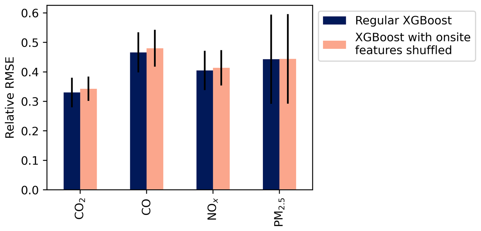
Figure 8 Relative RMSE for XGBoost-predicted C_bkg with and without covariates specific to the highway field site included in model. RMSE was calculated via 5-fold cross-validation; relative RMSE is RMSE divided by the standard deviation of the target regressand (C_bkg). Whiskers are standard deviations across folds.

The errors in Fig. 8 suggest that removing information specific to the highway site did not produce a significant change in XGBoost model accuracy. The absolute percent difference between RMSE with and without site-specific variables shuffled was less than 5 % for all pollutants, and differences were within 1 standard deviation across cross-validation folds, indicating little or no significant difference between models with and without shuffled site-specific variables. This indicates that most of the variability in C_bkg was explained by highway downwind concentrations and other covariates not specific to the highway – it is also reflective of our observations in Fig. 7 (and figures in Appendix H) that predicting C_bkg with concentrations measured at the Downsview urban background station, while less accurate than some other methods, still produced prediction R² exceeding 0.5 for all pollutants. Since concentrations measured at Downsview and the highway were included as predictors in both cases in Fig. 8, we can indirectly conclude that concentrations measured at Downsview coupled with concentrations measured downwind the highway together contain most of the information necessary to accurately predict C_bkg and that adding more emissions-source-specific covariates only marginally increased prediction accuracy.

This lack of difference between XGBoost accuracy with and without site-specific features might imply our model of background concentrations is not site-specific. That is, the XGBoost model without highway-specific covariates might be transferable to other locations. This in turn would mean that the spatial variation of background across the city is mostly encompassed within information provided by measuring the total concentrations at different sites, consistent with the assumption underlying frequency-based methods. With only one near-source site in this study with up- and downwind measurements, we did not further test this transferability. At the very least, this result shows our methodology might be successfully repeated at new near-source sites without requiring as many site-specific covariates as we included here.

3.4 Regression model feature importance

We can examine feature importance in the XGBoost models for each pollutant to gauge covariate importance for estimating C_bkg. We achieve this using Shapley additive explanations (SHAP) – SHAP plots can provide explanations of feature importance for complex nonlinear models where simple coefficients are not available, as is the case with XGBoost (Lundberg and Lee, 2017). Additional examples of SHAP values in the context of air pollution research can be found from Xu et al. (2020a, b). Figure 9 shows SHAP beeswarm plots for the XGBoost model predicting highway upwind background C_bkg for each pollutant.

Figure 9 SHAP beeswarm plots for XGBoost models predicting upwind background concentration at the highway site. These figures indicate relative degree of importance – for example, a blue dot far to the right on a feature indicates that a low value of that feature was associated with a high predicted concentration. Each dot represents one predicted concentration and one value of that feature (bkg: background; dv: Downsview; hwy: highway; meas: measured).

The SHAP values in Fig. 9 suggest that for CO, CO₂, and NO_x, the most important predictors of upwind background at the Highway 401 site were concentrations measured at the Downsview urban background site and hour of day. This is consistent with each of our prior discussed results: generally, concentrations measured at Downsview can provide a fair estimate of mean background concentration levels, but these estimates may be inaccurate during some hours of the day, and predictions can be notably improved through inclusion of additional information. The fact that time of day is an important predictor aligns with our observation that Downsview serves as a fair background estimate, except during morning and to a lesser degree evening rush hours (i.e. except during some hours of the day). Outside these important predictors, meteorology had notable importance for all pollutants. Lastly, for PM_2.5 pollutant concentrations measured at Downsview, while still important, had a lower impact on predictions, which is yet again reflective of the difficulty in predicting background PM_2.5 at the highway site.

Concentrations measured downwind the highway, C_meas, were much less important predictors in XGBoost than concentrations measured at Downsview. This was unexpected both based on theory and when comparing against other methods: C_meas should always be a direct sum of C_bkg and local emissions, and thus we expect it to explain some variability in background concentrations. This result was also in contrast to regression coefficients from our linear elastic net fits, which fit large coefficients on C_meas for all pollutants (Appendix L). Regardless, the results of this SHAP analysis suggest that C_meas had a comparatively small impact on XGBoost predictions. On the other hand, we found that our frequency methods, which take only C_meas as an input, had fair accuracy. These two results together suggest that to extract useful estimates of C_bkg from C_meas, algorithmic methods benefit by considering not just concurrent measurements but past and future values of C_meas as well. In this study, we did not include lagged values of C_meas in regression models, so further exploration of such covariate transformations might benefit C_bkg prediction accuracy and understanding of background concentration behaviour.

The importance of temperature for some predictions might be explained by an uneven distribution of measured temperatures. Most of our measurements occurred in winter with low temperatures, while a minority of measurements at the end of our study had higher temperatures. Because there are fewer samples with high temperatures, regression models risk placing a greater relative importance on those samples, inflating the relative importance of temperature. This can be improved upon in future studies by extending a similar regression fitting approach to a longer measurement period.

3.5 Limitations of analysis

As this study examined only a single urban area, the applicability of our results to other urban areas relies on the assumption that many cities feature a similar variety and heterogeneity of emissions sources and geography. The sites explored here, including both urban background and near-road up- and downwind sites, represented a variety of geographic features, including proximity to a large body of water, green space, and proximity to emissions sources other than the road targeted at the highway site. While our analysis of XGBoost model accuracy without site-specific features in Fig. 8 lends support to the idea that our model of background concentrations is not specific to the highway site, this conclusion is indirect and a better method of testing transferability would be to apply our methods at new sites.

We also only explored background concentrations for four airborne pollutants: three gaseous and one particulate. For the gaseous pollutants tested, we expect that loss or formation via reaction will be low. While NO and NO₂ concentrations can vary rapidly near roads through reaction, we only considered the sum of the two, NO_x, which should remain constant over the distances from the highway investigated here. This simplicity of behaviour will simplify our models, and it is plausible that background pollutants with more complex reaction mechanisms or sources might require more covariates to accurately predict with regression models. For example, modelling background ozone would probably benefit from including insolation as an exogenous predictor.

Lastly, it remains unclear if these models would transfer well to sites with different geometry, emissions sources, or weather. It is plausible that the strength of the methods tested here is due to the simplicity of the major source observed: the size and business of Highway 401 lends confidence to the assertion that it will be the dominant source of local airborne pollution at the downwind highway site. Traffic also has consistent diurnal patterns, and emissions intensity is easily inferred through a simple traffic count, which itself has a strong diurnal pattern. If the regression models presented here were refit near a source with different characteristics, such as an industrial source emitting at all hours of the day, or at a measurement site with multiple strong upwind sources, it stands to reason that predictive performance would be degraded.

4 Conclusions and recommendations

Based on the results of this study, we recommend that municipalities or air pollution specialists deploying sensors or monitors with the aim of resolving the contribution of specific emissions sources consider carefully how they will measure or algorithmically isolate the contribution of background to total measured concentrations. Our sites in Toronto reflected a variety of geographic features (varying built environments, water proximity, green space, etc.), indicating that our finding of varying background concentrations might apply to other cities, since these features are common across many urban areas. From our analysis of background concentration prediction methods, we can recommend which method users should choose based on their use case and availability of data. These recommendations are loosely ordered by decreasing strength of accuracy alongside decreasing cost:

1. If possible, direct measurement of background concentrations and wind immediately upwind the source of interest should always be preferred.

2. In cases where measurements of upwind C_bkg are available for some but not all of the study period, we recommend applying a regression approach. XGBoost or similar machine learning approaches are preferable to traditional regressions, as they allow for nonlinearity and unspecified interactions. Conversely, we caution against applying regression models outside the conditions they were trained in, such as different sites or seasons.

3. For applications where only long-term averages (i.e. 24 h or longer) are of concern, using a distant urban background station as a proxy for true on-site C_bkg measurements will prove sufficiently accurate; however, for higher-resolution measurements, urban background stations may prove inaccurate during periods of peak emissions, like during rush hour near a roadway.

4. For applications where both upwind C_bkg measurements and a suitable urban background station are both unavailable or too costly, we suggest applying one of the frequency methods described here, particularly the pseudo-wavelet method developed by Wang et al. (2018) or the rolling ball algorithm. For these frequency methods, in roadway applications we suggest using hyperparameters like those identified here (see Appendix K). For pollutants other than those measured here, we suggest applying parameters like those we identified, based on similarity in pollutant behaviour – for example, if a pollutant is expected to be a strong tracer or a local source, as NO_x is for traffic, we suggest applying similar hyperparameters as used for NO_x in this study.

5. In a similar vein, for cases where municipalities are deploying networks of sensors or epidemiologists are exploring geographic variability of background concentrations vs. local emissions, we suggest applying the pseudo-wavelet or rolling ball frequency methods. While the context of our tests here were up- and downwind differences targeting a single roadway emissions source, the theoretical basis of frequency methods – that background concentrations vary on a longer timescale than local emissions – extends these methods to pollution concentrations regardless of proximity to one particular source. The pseudo-wavelet method applied in this context is also touched upon by Wang et al. (2018) and Hilker et al. (2019).

Generally, we do not suggest applying the naïve rolling minimum method – superior frequency methods only require minimal additional computational cost. The usefulness of the ensemble method is also dubious. While the ensemble model did produce the best output in this case, this is to be expected; an ensemble model should outperform its constituent models. However, the extent of information and effort required to implement such a model for predicting C_bkg seems to exceed the potential benefit of gains in predictive accuracy. Finally, we suggest any study targeting specific emissions sources carefully consider how to extract local versus background contributions to measured concentrations, including but not limited to applying one of the methods tested here. We also encourage additional research in separating local and background concentrations, especially with different emissions sources or regions or for different types of measurements, such as mobile monitoring or distributed sensor networks.

Appendix A: Micrometeorological and other inputs for RLINE

We used the RLINE model to produce dispersion estimates as an input feature for regression models in this study (Snyder et al., 2013). The RLINE model uses outputs from the AERMET micrometeorological pre-processor produced by the United States Environmental Protection Agency (U.S. EPA, 2004). AERMET requires a variety of micrometeorological measurements as inputs, which can be provided in a variety of formats. We employed measurements from Toronto's Pearson International Airport, acquired from the National Centers for Environmental Information Integrated Surface Database (National Centers for Environmental Information, 2025), and upper air measurements at Buffalo Niagara International Airport, acquired from the National Oceanic and Atmospheric Administration's radiosonde database (National Oceanic and Atmospheric Administration, 2024).

We identified lane and receptor geometry using ArcGIS Pro and Google Earth Pro. We set initial vertical dispersion, σ_z,init, using the recommended formula in the RLINE user manual, which in turn points to EPA guidance (Environmental Protection Agency, 2010; Snyder and Heist, 2013). This formula uses vehicle heights and fleet mix to estimate initial dispersion – we assumed vehicle heights of 1.5 m for light-duty vehicles and 4.15 m for medium- and heavy-duty vehicles, based on the same EPA guidance document and the law in Ontario governing maximum vehicle height (Ontario, 2012). Other inputs were taken from recommendations in the RLINE user manual.

Appendix B: Data processing

Analysis code and raw data can be made available upon request. Data​​​​​​​ processing was conducted primarily in Python, including the open-source library pandas (https://doi.org/10.5281/zenodo.3509134, The pandas development team, 2020), numpy (Harris et al., 2020), matplotlib (Hunter, 2007), scipy (Virtanen et al., 2020), patsy (https://doi.org/10.5281/zenodo.10459707, Smith et al., 2024), statsmodels (Seabold and Perktold, 2010), seaborn (Waskom, 2021), shap (Lundberg and Lee, 2017), windrose (https://doi.org/10.5281/zenodo.13133010, Celles et al., 2024), xgboost (Chen and Guestrin, 2016), optuna (Akiba et al., 2019), cmcrameri (https://doi.org/10.5281/zenodo.8409685, Crameri, 2023), tqdm (https://doi.org/10.5281/zenodo.14231923, da Costa-Luis et al., 2024), scikitlearn (Pedregosa et al., 2011), and scikit-image (van der Walt et al., 2014).

To ensure air pollutant concentration measurements were accurate, realistic, and comparable between sites, we performed an extensive quality assurance and control process on the raw measurements prior to use. First, gas-phase instruments at the Downsview, Hanlan's, Wallberg, and Highway 401 south sites are calibrated regularly.

Prior to analysis, we applied the following steps to raw measurements:

1. We removed periods identified as invalid measurements in our measurement database for reasons such as calibration or maintenance. In some cases, we dropped additional measurements if it appeared the instrument was turned back on too soon after calibration.

2. We manually removed some periods that appeared to have extreme outliers or unusual behaviour suggestive of instrument malfunction, calibration problems, or transient spikes unrelated to the measured road emissions or background concentrations.

3. We corrected PM_2.5 measurements from the AirSENCE instrument for interference from humidity with the correction equation suggested by Crilley et al. (2018).

4. We corrected for baseline drift in CO₂ measured at Hanlan's Point, Wallberg, and both Highway 401 stations by assuming concentrations measured at these sites must be similar to CO₂ measured at the Downsview site occasionally over a 48 h period. We selected the Downsview urban background station as the reference site for this adjustment because it was calibrated during the sampling campaign. We applied such a correction specifically by calculating the rolling 48 h 0.1 % quantile of each CO₂ signal and assuming these rolling quantiles must be equal – we then added the difference between the Downsview quantile and each site's rolling quantile to the CO₂ signal at each site (except Downsview, since it was treated as the reference). We applied a similar baseline correction for CO only at the Hanlan's site, as this site's CO measurements began drifting near the end of the measurement period.

5. We calibrated the Highway 401 background AirSENCE instruments by placing the sensor package on the roof of the Highway 401 south station for nearly 18 d prior to deployment to the north side of the highway. With these 18 d raw pollutant measurements, we calibrated the AirSENCE instrument against measurements from the south station's reference instruments. This calibration was specifically a linear regression, regressing a target function like the following:

   $$\begin{array}{}\text{(B1)}& \begin{array}{rl}{C}_{\mathrm{ref}}& ={\mathit{\beta }}_{\mathrm{0}}+{\mathit{\beta }}_{\mathrm{1}}{C}_{\mathrm{AS}}+{\mathit{\beta }}_{\mathrm{2}}T+{\mathit{\beta }}_{\mathrm{3}}P+{\mathit{\beta }}_{\mathrm{4}}\mathrm{RH}\\ & +{\mathit{\beta }}_{\mathrm{5}}{C}_{\mathrm{AS}}T+{\mathit{\beta }}_{\mathrm{6}}{C}_{\mathrm{AS}}P+{\mathit{\beta }}_{\mathrm{7}}{C}_{\mathrm{AS}}\mathrm{RH},\end{array}\end{array}$$

   where C_ref denotes concentrations recorded by the reference instruments, C_AS denotes concentrations measured by the AirSENCE low-cost platform, T is ambient temperature, P is ambient pressure, RH is ambient relative humidity, and β denotes regression coefficients. We regressed this function for each pollutant and then created predicted values of C_ref for the entire measurement campaign and treated these values as calibrated measurements from the AirSENCE device after we deployed it to the north (background) side of the highway.

6. After the above steps, we set concentrations less than zero to 10⁻⁵ for each pollutant. We applied this adjustment to simplify analyses that required taking the logarithm of concentrations.

Table B1 shows some measures comparing AirSENCE pollutant concentrations to reference instruments at the Highway 401 south station before and after calibration. These measures generally appear to indicate that the AirSENCE reported similar concentration measurements to the reference instruments during the training period after measurements were preprocessed using steps 1 through 5 above.

Table B1 Statistics comparing concentrations measured by the low-cost AirSENCE sensor platform to reference instruments before and after calibrating the AirSENCE measurements.

The performance statistics in Table B1 imply that, after calibration, measurements captured by the low-cost AirSENCE sensors were comparable to those captured by the reference instruments, with small errors and effectively no bias for CO, CO₂, and NO_x. However, for PM_2.5, the fraction of values falling within a factor of 1.1 (A_F=1.1) and the RMSE imply that PM_2.5 measurements were relatively less accurate than other pollutants. This likely compounded with our observation of homogeneity in PM_2.5 background concentrations in the Toronto region, further reducing our ability to separate C_bkg from C_meas for PM_2.5 at the Highway 401 site. Accordingly, and as mentioned in the main article body, our ability to extract meaningful results at the Highway 401 site was lower for PM_2.5 than for other pollutants. However, our observation that PM_2.5 was largely homogeneous across Toronto remains valid, as the low-cost AirSENCE device was only deployed at the highway upwind background site.

Appendix C: Descriptions of background concentration prediction algorithms

The following sections list the various frequency- and regression-based algorithms we tested for estimating on-site upwind background concentrations. Most methods follow a similar optimization scheme, and all were tuned to produce the best possible estimate of measured background, C_bkg, at the highway upwind background site.

Except where otherwise noted, we applied a similar optimization method for tuning and fitting each of these algorithmic models. We employed the Optuna Python library, which applies Bayesian hyperoptimization to search the possible space of hyperparameters for an optimal configuration (Akiba et al., 2019). For scoring during optimization, we calculated the 5-fold cross-validated root mean square error (RMSE) of predictions. In stratified cross-validation, the model is fit or regressed to most of the data (the training set) while a subset is held aside (the test set). After fitting, predictions are generated for the held-out test set and compared to the target variable in that set. In this study, this means the regression model is fit to $\mathrm{4}/\mathrm{5}$ (80 %) of the measurements, and then predictions are made using the remaining $\mathrm{1}/\mathrm{5}$ (20 %) of measurements, and we calculated the RMSE of those predictions. The mean RMSE across all 5 folds is then taken as the score for that hyperparameter configuration, and the set of parameters with the lowest RMSE after some predefined number of optimization trials is selected as the optimal model.

For frequency-based methods, the concept of creating predictions for a held-out set is less meaningful, because these methods use information in the input C_meas signal across a span of times to produce their C_bkg predictions, so holding out some data is challenging. However, to produce an RMSE score that was more comparable to that for regression methods, we produced a frequency-method C_bkg prediction for all measurements, then calculated the RMSE for the indices associated with each of the 5 cross-validation folds, and then took the mean of those 5 RMSE scores as the final score for that optimization trial. In this way, the score was a mean of scores, similar to the cross-validation approach in regression methods. We applied this same mean-of-fold's-scores approach when evaluating frequency-method predictions as in Figs. 7 and H1–H3. We also limited evaluation of frequency methods to use only those measurement periods where regression methods were also evaluated. We do this because the large number of predictors in regression methods gives rise to some gaps in the feature set that are not included during regression – using only those times made available to regression methods ensures a fair comparison between background stations, frequency methods, and regression methods.

We prioritized the RMSE as our regression metric due to its popularity in the literature and because it produces an error in units of the target concentration (i.e. ppmv, ppbv, or µg m⁻³). However, we note that other metrics might produce superior model fits due to their statistical advantages. In particular, the mean squared log error (MSLE) has advantages for air pollution research, on the basis that atmospheric pollution concentrations are bounded and not normally distributed. Airborne concentrations are typically log-normally distributed, meaning a prediction error underestimating the true concentration must be bounded between zero and the true concentration, while an overestimating prediction has no upper bound. This uneven bounding means algorithms attempting to minimize the RMSE of airborne concentrations are more likely to produce a prediction that underestimates than overestimates, because the RMSE penalizes positive and negative errors equally, but only positive errors are unbounded. The MSLE, on the other hand, more strongly penalizes underestimations because it log-transforms the target and prediction, which is appropriate for air pollution concentrations where underestimations are more likely to be small due to their bounded nature. Despite these advantages, we retained the RMSE as our primary metric for the reasons mentioned above. Also, a reader can immediately understand an RMSE score in the context of typical real-world pollutant concentrations: an RMSE of 10 ppmv for a CO₂ prediction is understandable relative to typical real concentrations above 400 ppmv, but a MSLE of 0.001 log-ppmv is not intuitive.

The following sections describe each algorithmic C_bkg prediction method in detail.

C1 Naïve rolling minimum

Baseline or background concentrations in the literature are frequently estimated as a concentration that is less than and occasionally but not always equal to the total measured concentration – in other words, the background concentration is taken to loosely follow the lower limit of measured concentrations, while transient peaks are attributed to local sources. Examples of such approaches include those applied by Klems et al. (2010), Sabaliauskas et al. (2014), and Hilker et al. (2019). Similar approaches are also applied in other fields, such as removing baseline signals in spectroscopic signals, which share some similar characteristics to pollutant concentration signals.

Other than taking the absolute minimum measured concentration as a baseline, the next simplest approach is to consider a rolling minimum over some period of continuous measurements. Thus, a rolling minimum background has only one parameter to tune: the width of the rolling window. We considered possible window widths in the range of 5 min to 48 h. Because of the simplicity of this approach, we did not apply Bayesian hyperoptimization and instead tested all window widths in this range in 5 min increments.

We did not expect the naïve rolling minimum model to produce reasonable estimates of background concentration. Instead, we intended this method to serve as a bar by which to judge the remaining, more sophisticated algorithmic predictions.

C2 Pseudo-wavelet

The pseudo-wavelet method estimates a background concentration similarly to wavelet methods à la Klems et al. (2010) and Sabaliauskas et al. (2014), but it is not a true wavelet algorithm. At a high level, the pseudo-wavelet algorithm produces multiple interpolations between the two smallest values of measured downwind concentrations within a rolling window of varying widths and then averages these interpolations to produce a smoothed estimate of background concentration. The algorithm requires three inputs: the measured total pollutant concentrations, C_meas; the initial width of the rolling windows, W, in units of the C_meas measurement frequency, which in this case was minutes; and a unitless smoothing parameter, α.

Additional detail and applications of the pseudo-wavelet algorithm are provided by Wang et al. (2018), where it was originally introduced, and by Hilker et al. (2019), who evaluated background concentration predictions produced by the pseudo-wavelet method against some other methods.

C3 Rolling ball

The rolling ball method simulates sliding a ball along the bottom of the measured total pollutant signal, with the background being the trace defined by the path of the top of the ball. This approach is common in image processing to remove uneven or noisy image backgrounds. We are not aware of any implementations of this method in air quality studies, but background concentrations predictions from the rolling ball algorithm have similar properties to those from the pseudo-wavelet algorithm. The rolling ball method requires three inputs: C_meas and two tuning parameters defining the shape of the ball.

In air pollution data, the horizontal axis of the C_meas signal is in units of time, while the amplitude is in units of pollution concentration. Accordingly, the rolling ball algorithm in practice is more accurately described as sliding an ellipsoid along the bottom of the C_meas signal, with the dimensions of the ellipsoid being defined in different units from each other. The semi-major axis of the ellipsoid will align with the concentration (vertical) axis of the pollutant signal and have units of concentration, while the semi-minor axis will align with the temporal (horizontal) axis and have units of the pollutant signal's frequency – in this case, minutes. Thus, the rolling ball algorithm requires two tuning parameters which are these semi-axis lengths. To simplify this algorithm, we fixed the length of the concentration semi-axis as equal to the standard deviation of the total measured downwind concentration, C_meas, of the relevant pollutant. This reduced the number of parameters needing tuning to one. We optimized this remaining parameter, the length of the temporal semi-axis, via hyperoptimization. We considered possible widths in the range of 2 min to 48 h.

C4 Regression model covariates

Regression-based methods incorporated both the measured highway downwind concentration signal alongside additional predictor variables to estimate upwind background concentrations. They do not incorporate the time-series nature of the measurements, using only concurrent values of each covariate to estimate background. We did not develop these regression models from a theoretical basis but from a primarily statistical basis – we selected covariates for their potential to improve estimates regardless of any possible physical interpretation of their effect in a regression model.

The covariates included in each of the base regression models were the following:

• total concentrations measured downwind the highway, C_meas, in units matching the pollutant;

• concentrations measured at the two urban background stations, C_bkg,dv and C_bkg,hanlans, also in units matching the target pollutant;

• counts of vehicles on the highway in each minute, N, in units of vehicles min⁻¹, and a weighted average vehicle speed, in km h⁻¹ (Only the nearest 8 of 17 lanes on the highway were captured by a radar counter.);

• RLINE dispersion predictions, k_hwy, in units of s m⁻²;

• squared cosine and sine of wind direction measured at the highway, cos ²(θ), sin ²(θ);

• wind speed measured at the highway, u, in m s⁻¹, taken as the inverse ($\mathrm{1}/u$);

• ambient temperature measured at the highway, T, in °C, squared;

• ambient pressure measured at the highway, P, in hPa;

• ambient relative humidity measured at the highway, RH, in %;

• hour of day and day of week encoded as one-hot columns for OLS and elastic net and as integers for XGBoost.

Concentrations measured at Downsview are denoted with the subscript dv and Hanlan's Point with the subscript hanlans.

We included meteorological measurements from only the highway site; however, when testing the importance of highway site-specific regression features in Sect. 3.3, we did not permute meteorology variables because these values tend to be strongly correlated at sites across the city and are thus not site-specific in the sense that we sought in this analysis. The purpose of testing highway site-specific feature importance was to indirectly test model transferability, and since meteorology should be similar across sites, it does not need to be considered a site-specific feature.

For all regression models, we scaled covariates to zero mean and unit variance before fitting.

C5 Ordinary least squares regression

As a first-pass regression model we employed a simple ordinary least squares (OLS) multiple linear regression, with each of the above-listed covariates as exogenous regressors. While we do not necessarily expect the relationship between measured background concentrations and any particular covariate to be linear, we included a linear regression estimate due to the familiarity and popularity of such models in the literature.

We expect regularized and non-linear machine learning models to match or outperform OLS for all pollutants. As the naïve rolling minimum sets the bar for accuracy for all algorithmic estimates, the OLS model sets a second hurdle by which to judge more sophisticated regression models.

C6 Regularized (elastic net) regression

Elastic net regression is a linear model like OLS but applies additional penalties to model loss during fitting based on the size of regression coefficients, essentially preferring more parsimonious models with smaller coefficients. Elastic net specifically includes both L1 and L2 regularization terms, which when applied individually would be referred to as lasso and ridge regression, respectively. The L1 penalty shrinks coefficients towards zero, penalizing large coefficients and performing variable selection. The L2 penalty shrinks large coefficients asymptotically towards zero. Applying these penalties to a linear regression model retains the interpretability of linear regression coefficients but reduces the risk of overfitting through both variable selection and coefficient shrinking. In this application, we expect the elastic net regression to outperform OLS because we test our background concentration estimates through cross-validation, which will help identify models that overfit to training data. We selected the degrees of L1 and L2 regularization through hyperoptimization.

C7 Machine learning with XGBoost

Machine learning allows for non-linearity and feature interactions in the underlying relationship between true background and covariates. However, the downsides are a risk of overfitting, challenging tuning, and reduced interpretability.

XGBoost has many hyperparameters to tune that can individually and together strongly influence model performance. We selected some hyperparameters to tune and others to hold constant based on trial and error. We optimized maximum tree depth, number of boosting rounds, learning rate, L1 and L2 regularization, and XGBoost's gamma regularization term. We held other parameters constant at either their default values or at values selected through trial and error and case knowledge. We set minimum and maximum bounds for hyperparameter optimization based on best judgement and again through extensive trial and error.

C8 Ensemble background estimate

As a final algorithmic C_bkg prediction model, we considered an ensemble of predictions from each of the methods introduced thus far. Our ensemble model was an L2-regularized (ridge) regression taking each of the other estimated backgrounds (two urban background stations, three frequency methods, and three regression methods) as exogenous variables, along with an intercept. The ensemble regression did not include the covariates listed above that were included in the base regression models, instead taking the outputs of the other models as inputs. We selected the degree of L2 regularization for the ensemble model by searching 160 logarithmically spaced values from 10⁻⁹ to 10⁷, rather than through randomized Bayesian hyperoptimization.

Appendix D: Meteorology at the highway field site

Figure D1 Mean diurnal patterns of wind speed (u), temperature (T), pressure (P), and relative humidity (RH) measured at the Highway 401 downwind south station.

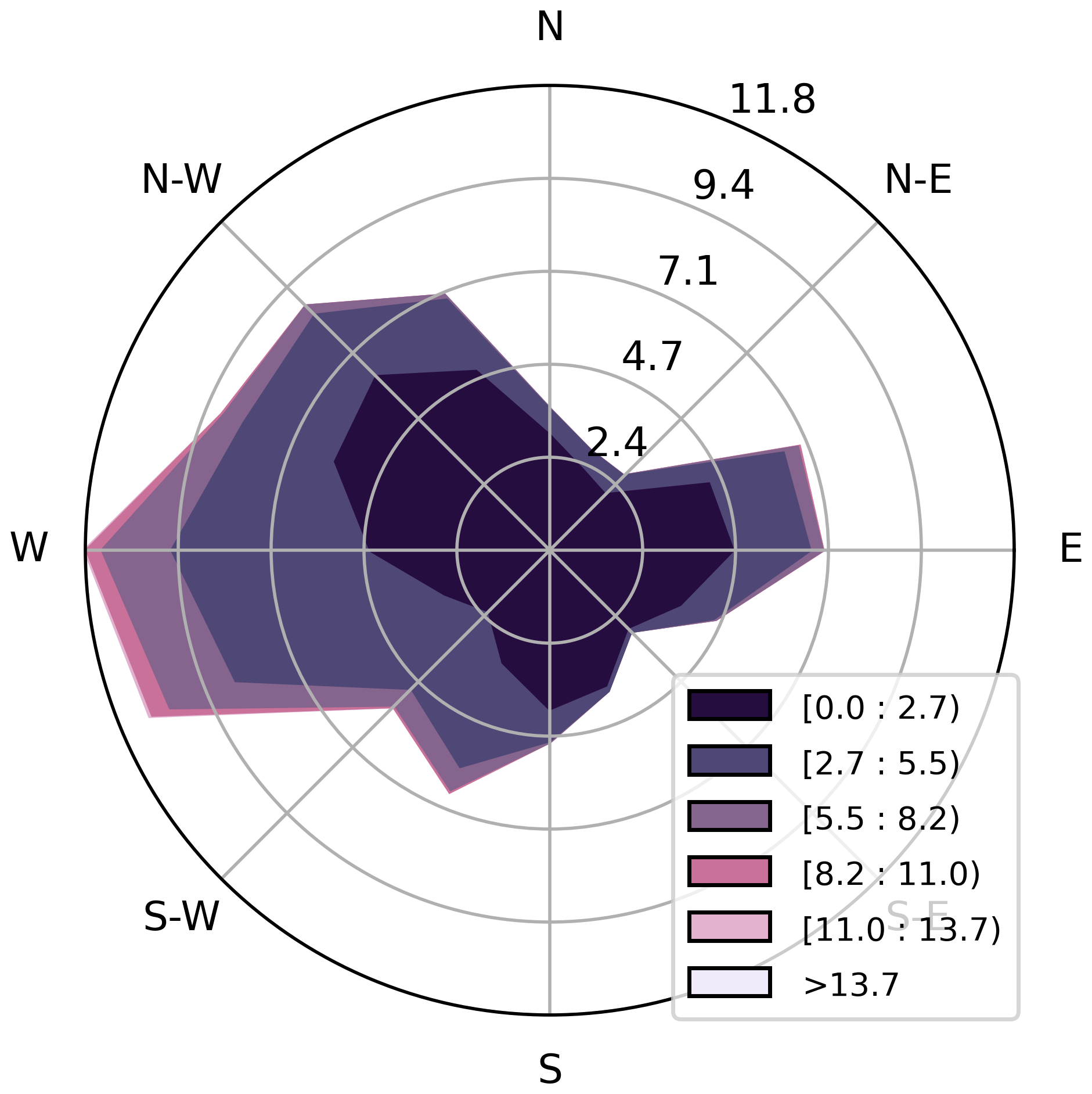
Figure D2 Wind rose depicting dominant wind speeds and directions at the Highway 401 field study location, measured on the south and predominantly downwind side of the highway.

Figure D3 Diurnal heatmap depicting frequency of wind directions measured on the south side of Highway 401 over the entire study period. The dashed red line indicates the direction that would be directly perpendicular and across the road at the measurement point.

Appendix E: Comparing SHARP and T640 instruments

Figure E1 Scatter matrix comparing SHARP and T640 instruments across three of the sites used in this study. Red lines are 1:1; dashed lines with shaded areas are linear regressions with 95 % confidence intervals. Diagonal histograms are kernel density estimates with areas summing to unity – y axes on these subfigures are in units of density, omitted to avoid figure clutter.

Appendix F: Separating local and background signals by wind speed and direction

Figure F1 shows background and roadside downwind concentrations at Highway 401 as a function of concurrent wind direction. From this figure, we identified the wind directions appropriate for considering the background sensor north of the highway to be a true measure of C_bkg. As indicated in the methodology, the range we selected was between 80° to the northwest and 40° to the northeast – these directions correspond to approximately 260 and 60° with respect to north, with the offset of 20° accounting for the angle of the highway. We chose these limits based largely upon the ranges where the difference in down- and upwind sensors (i.e. $C_{\mathrm{local}}=C_{\mathrm{meas}}-C_{\mathrm{bkg}}=\mathrm{\Delta }C)$ began to trend towards zero.

In addition to decreasing mean concentrations concurrent with the higher wind speeds as discussed in the methodology and visible in Fig. F2, we also observed an unexpected maximum mean C_local for some pollutants at wind speeds ∼ 2 m s⁻¹. This was most apparent for NO_x but was also present to a lesser extent in CO and CO₂. The cause of increasing C_local at wind speeds below 2 m s⁻¹ is not clear. With all other variables (meteorology, emissions, etc.) held constant, simple dispersion theory predicts decreasing local concentrations associated with increasing wind speeds. There are some possible explanations for this observation: higher wind speeds typically occur during midday to afternoon when insolation is greatest, which is concurrent with higher anthropogenic activity and thus emissions. This possibility is supported qualitatively by Fig. F3, which shows similar trends of C_local as a function of wind speed but with the underlying measurements coloured by time of day also shown. In these figures, we observed that higher wind speeds and higher concentrations both tended to occur later in the day – more green points are to the right of the axes in Fig. F3, indicating that we recorded higher wind speeds more often later in the day. These simultaneous correlations lend themselves to the appearance of a positive correlation between wind speed and C_local. This can be corroborated by comparing the diurnal trends of C_local in Fig. I1 and wind in Fig. D1, where we observed high average concentrations during the same times of day as high average wind speeds.

Figure F1 Median pollutant concentrations at the Highway 401 site binned by concurrent wind direction in 1° bins. The difference (Δ) between the measured (red) and background (blue) concentrations is shown in black on the secondary y axis. Wind direction is adjusted so zero is directly normal and facing across the road from the roadside downwind measurement site. The highway lays mostly east–west, so positive directions indicate more easterly winds, and negative directions indicate more westerly winds. Trends were smoothed and interpolated with a weighted centred rolling mean across 15 adjacent increments, weighted by sample size.

Figure F2 Mean pollutant concentrations at the Highway 401 site as a function of concurrent wind speed. Trends were generated by first calculating mean concentrations within 0.1 m s⁻¹ bins of concurrent wind speeds. Increments with fewer than 60 measurements were excluded. Trends were smoothed and interpolated with a weighted centred rolling mean across 11 adjacent increments, weighted by sample size. For C_local, we only included periods where C_local>0 when producing these trends.

Figure F3 Mean pollutant concentrations at the Highway 401 site as a function of concurrent wind speed. Mean trends were generated by taking mean concentrations within 0.1 m s⁻¹ bins of concurrent wind speeds. Points are underlying measurements used to generate the trends and are coloured by hour of day the measurement fell within. We only included periods where C_local>0 when producing these scatters and trends.

Appendix G: Exemplar time-series trends

Figure G1 Example of measured and estimated background pollutant signals at the Highway 401 field study site. For clarity, not all background estimation methods are shown here. Grey-shaded regions indicate when the south site was downwind the highway, indicating periods where the C_bkg signal was a valid measurement of background concentration as defined in the methodology.

Appendix H: C_bkg prediction accuracies for NO_x, CO₂, and PM_2.5

Figure H1 Root mean square error (RMSE, bars) and coefficient of determination (R², diamonds) for predicted background NO_x at the highway site, as predicted by each method tested here. Scores show the accuracy of each method in estimating true upwind background concentration, with lower RMSE and greater R² being better. Scores were calculated as the mean across 5-fold cross-validation.

Figure H2 Root mean square error (RMSE, bars) and coefficient of determination (R², diamonds) for predicted background CO₂ at the highway site, as predicted by each method tested here. Scores show the accuracy of each method in estimating true upwind background concentration, with lower RMSE and greater R² being better. Scores were calculated as the mean across 5-fold cross-validation.

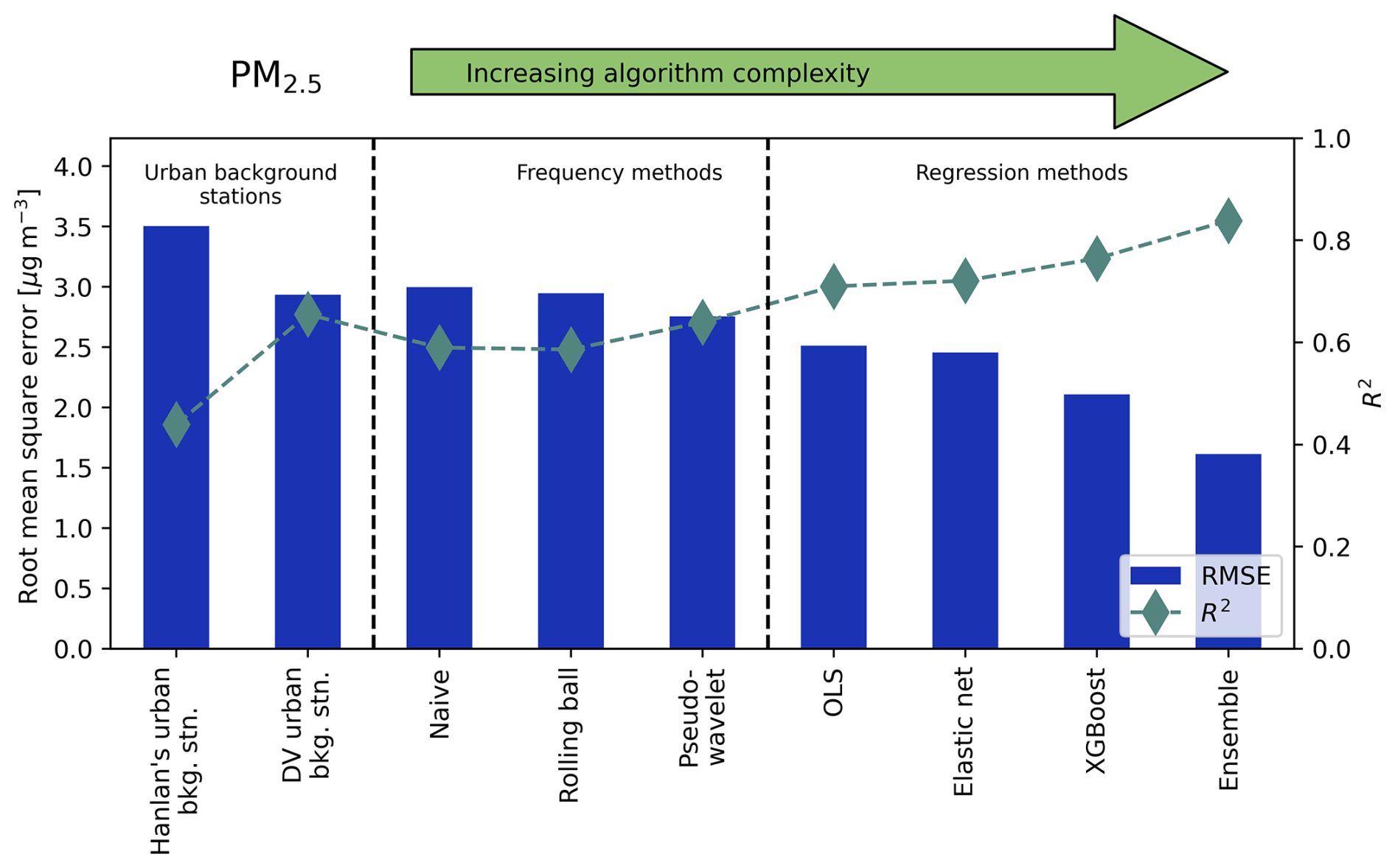
Figure H3 Root mean square error (RMSE, bars) and coefficient of determination (R², diamonds) for predicted background PM_2.5 at the highway site, as predicted by each method tested here. Scores show the accuracy of each method in estimating true upwind background concentration, with lower RMSE and greater R² being better. Scores were calculated as the mean across 5-fold cross-validation.

Appendix I: C_local diurnal patterns

Figure I1 Mean hourly diurnal trends of the difference between measured concentrations downwind the highway (C_meas) and background concentrations upwind of the highway (C_bkg) for each pollutant. Periods where the difference, C_local, was negative were excluded. When producing these trends, we limited data to periods where the sensors were up- and downwind of the road but did not apply limits to wind speed.

Appendix J: Background concentration scatters

Figure J1 Paired scatters and kernel density estimates (KDEs) of background carbon monoxide concentrations at three stationary measurement sites in the Greater Toronto Area. Red lines are 1:1. For the Highway 401 site, backgrounds were only considered valid when wind direction and speed fell within the ranges specified in the methodology; figures only show periods where backgrounds were concurrently measured at each site. To speed calculation of the KDE and lower figure density, a random 10 % subset of measurements are shown here.

Figure J2 Paired scatters and kernel density estimates (KDEs) of background nitrogen oxides (NO + NO₂) concentrations at three stationary measurement sites in the Greater Toronto Area. Red lines are 1:1. For the Highway 401 site, backgrounds were only considered valid when wind direction and speed fell within the ranges specified in the methodology; figures only show periods where backgrounds were concurrently measured at each site. To speed calculation of the KDE and lower figure density, a random 10 % subset of measurements are shown here.

Figure J3 Paired scatters and kernel density estimates (KDEs) of background particulate matter < 2.5 µm diameter concentrations at three stationary measurement sites in the Greater Toronto Area. Red lines are 1:1. For the Highway 401 site, backgrounds were only considered valid when wind direction and speed fell within the ranges specified in the methodology; figures only show periods where backgrounds were concurrently measured at each site. To speed calculation of the KDE and lower figure density, a random 10 % subset of measurements are shown here. Note that the Hanlan's Point site used a different PM_2.5 instrument – see methodology for details.

Appendix K: Frequency method optimized hyperparameters

While frequency methods were often less accurate in predicting C_bkg than regression methods, they can provide insight into background pollutant behaviour by examining their optimized hyperparameters. For the naïve rolling minimum and rolling ball algorithms, both were fit with a single hyperparameter, and in both cases this single parameter expresses an effective width of temporal duration of measured roadside downwind concentrations to consider when estimating background concentrations. For the naïve rolling minimum, the tuned parameter is the window width in minutes, and for the rolling ball axis it is the radius along the temporal semi-axis of the ellipse that is “rolled” along the bottom of the downwind pollution concentration signal. For both, a larger parameter produces a predicted C_bkg that has less or slower temporal variability and a lower average magnitude. For the pseudo-wavelet method there are two parameters that are somewhat interchangeable in how they affect the resulting C_bkg prediction, but they can be similarly interpreted because larger values again produce more slowly varying and smaller signals.

Table K1 shows the hyperoptimized best parameters for each frequency method. The differences between optimized parameters reflected the characteristics and spatial variability of the pollutants – particularly the order of pollutants as ranked by frequency method coefficients loosely correlated with pollutants as ordered by their coefficients of variation (CVs) in Table 2. NO_x and PM_2.5 had the largest hyperparameters across methods and the greatest CVs, followed by CO, and then CO₂. Another way to interpret these parameters is to consider that for all frequency methods, very large hyperparameters lead to background predictions that approach a constant value, so the relative size of these parameters indicates the extent to which the background concentration for that pollutant might be appropriately estimated as a constant value. Thus, these parameters provide additional, albeit indirect, evidence for differences in temporal variability of pollutant backgrounds relative to their means. This correlates with our prior observation that low NO_x background concentrations paradoxically make predicting NO_x C_bkg both easier and harder depending on the context.

For the pseudo-wavelet algorithm, the rankings of optimal α and W parameters were similar to the naïve minimum and rolling ball methods. Larger values of W produce background concentration predictions that vary more slowly and less frequently equal the input C_meas signal and thus make up a smaller portion of the total measured concentration. In other words, larger values of W indicate that local emissions are a more dominant driver of concentration variability. Similar conclusions can be drawn for values of α. However, to a certain extent W and α are interchangeable, as demonstrated by the examples in Hilker et al. (2019), so it is more challenging to draw meaningful conclusions about background concentration characteristics from the pseudo-wavelet algorithm's parameters than from the naïve and rolling ball methods, which each use a single and more easily interpreted tuning parameter. Despite this, we find a broad agreement across frequency methods in the relative magnitudes of optimized parameters between pollutants: these parameters suggest NO_x and PM_2.5 background concentrations varied less rapidly relative to their average levels than CO₂ and CO.

Table K1 Hyperoptimized parameters for the naïve rolling minimum, rolling ball, and pseudo-wavelet (PW) background estimation algorithms. Parameters are in units of minutes except α, which is unitless.

Appendix L: Elastic net regression coefficients

Figure L1 Elastic net regression coefficients for predicted highway upwind background CO. The optimal degree of L1 and L2 regularization was identified via 5-fold stratified cross-validation. Covariates were standardized prior to fitting, so coefficients are unitless.

Figure L2 Elastic net regression coefficients for predicted highway upwind background CO₂. The optimal degree of L1 and L2 regularization was identified via 5-fold stratified cross-validation. Covariates were standardized prior to fitting, so coefficients are unitless.

Figure L3 Elastic net regression coefficients for predicted highway upwind background NO_x. The optimal degree of L1 and L2 regularization was identified via 5-fold stratified cross-validation. Covariates were standardized prior to fitting, so coefficients are unitless.

Figure L4 Elastic net regression coefficients for predicted highway upwind background PM_2.5. The optimal degree of L1 and L2 regularization was identified via 5-fold stratified cross-validation. Covariates were standardized prior to fitting, so coefficients are unitless.

Appendix M: Example of cross-validation stratification

Figure M1 Train–test split with 5-fold cross-validation for predicting highway upwind background NO_x. This example figure demonstrates how measurements were split during cross-validation. In each fold, models were trained on measurements coloured blue and tested against measurements coloured orange. Black points demonstrate model-predicted background concentrations in each fold.