The added value and potential of long-term radio occultation data for climatological wind field monitoring

Global long-term stable 3D wind fields provide valuable information for climate-oriented analyses of the dynamics of the atmosphere. Their monitoring remains a challenging task given the shortcomings of available observations. One promising option for progress is the use of radio occultation (RO) satellite data, which enable deriving dynamics based on thermodynamic data. In this study we focus on three main goals, explored through the fifth version of the European Centre for Medium-Range Weather Forecasts (ECMWF) Reanalysis (ERA5) and RO datasets, using monthly-mean January and July data over 2007–2020. Our focus is on a 2.5° × 2.5° spatial synoptic scale over the free troposphere to the mid-stratosphere (i.e. 800–10 hPa). First, by comparing ERA5-derived geostrophic and gradient wind speeds to the original ERA5 ones, we examine the regions of validity of the studied approximations at a given synoptic-scale resolution. Second, to assess the possible added value of the RO-derived climatic winds in terms of their long-term stability, we test their consistency with the corresponding ERA5-derived winds. Third, by comparing the RO climatic winds to the original ERA5 winds, we evaluate the potential benefit of RO as an additional dataset for wind analyses and climate monitoring. With this three-step analysis, we decompose the total wind speed bias into the contributions from the approximation and the systematic difference between the RO and ERA5 datasets. We find that the geostrophic approximation is a valid method to estimate winds in the free troposphere, while the gradient wind approximation works better in the lower stratosphere. Both approximations generally work well over the mentioned altitudes, within an accuracy of 2 m s⁻¹ for the latitudes 5–82.5°. Exceptions are found in winter in the monsoonal area and above larger mountain ranges in the free troposphere, as well as above the northern polar regions in the mid-stratosphere. RO- and ERA5-derived geostrophic winds mostly showed good agreement (within 2 m s⁻¹). However, temporal change in the systematic difference higher than 0.5 m s⁻¹ per decade was found. This points to a possible impact of changes in the source of the assimilated data in ERA5. The overall high accuracy of the monthly-mean wind fields, backed by the long-term stability and fine vertical resolution of the underlying RO data, highlights the added value and potential benefit of RO-derived climatic winds for climate monitoring and analyses.

1 Introduction

Wind field measurements have an important role in numerical weather prediction (NWP) and in atmospheric sciences for understanding climate dynamics and chemistry. As they serve as initial conditions in NWP models, their accuracy is of great importance. Besides, such data are also regularly assimilated in reanalysis systems, contributing to advances in climate science (Stoffelen et al., 2005; Eyre et al., 2020). Even though nowadays there is an increased number of different techniques for measuring wind speeds, having accurate global 3D wind information is still a demanding task due to certain limitations of specific observation techniques (Stoffelen et al., 2005, 2020). While some techniques have generally good spatial coverage (e.g. meteorological stations, ships, buoys, scatterometer winds from satellite radars), they only provide wind information on single levels, lacking the vertical wind profile. On the other hand, techniques providing vertical profiles (e.g. wind profilers, radio-sounding data, pilot balloon data) have relatively coarse spatial coverage. Hence over larger parts of the Southern Hemisphere, such as oceans, obtaining both fine horizontal and fine vertical wind information is a problem (Stoffelen et al., 2005, 2020).

Altitude-resolving satellite data can help overcome these problems between profiling information and good global coverage. The European Space Agency (ESA) Earth Explorer mission Aeolus utilises the active Doppler wind lidar method to measure wind from the surface to 30 km altitude (Stoffelen et al., 2005; Kanitz et al., 2019). The assimilation of this dataset resulted in improvement in NWP forecasts (Rennie et al., 2021; Žagar et al., 2021), as well as helping to better understand and analyse atmospheric dynamics such as Kelvin waves (Žagar et al., 2021) or gravity waves (Banyard et al., 2021). However, due to its quite short time period (launched in August 2018), these data are not suitable for climate change analyses. Another technique to derive vertical profiles is global navigation satellite system (GNSS) radio occultation (RO), where the thermodynamic state of the atmosphere is obtained based on the transmitted GNSS radio signals refracted by the Earth's atmosphere (Kursinski et al., 1997; Steiner et al., 2011; Mannucci et al., 2020). The advantage of RO is its unique combination of global coverage, high vertical resolution, high accuracy, long-term stability and multi-mission data consistency (e.g. Anthes, 2011; Foelsche et al., 2011; Angerer et al., 2017; Zeng et al., 2019; Steiner et al., 2020a). The RO datasets are assimilated into operational weather forecasts (e.g. Healy and Thépaut, 2006; Buontempo et al., 2008; Cardinali, 2009) and long-term reanalyses (e.g. Hersbach et al., 2020; Kobayashi et al., 2015; Gelaro et al., 2017) and are used in climate analysis studies (e.g. Steiner et al., 2011, 2020b; Stocker et al., 2021).

While RO does not directly provide wind information, winds can be estimated from geopotential information using the conventional geostrophic and gradient wind approximations. The geostrophic approximation is a commonly used wind method in diagnostic studies. Although its utility in the mid-latitudes of the free troposphere was found to be good (e.g. Holton and Hakim, 2013; Boville, 1987; Randel, 1987), in the winter extratropical stratosphere, significant overestimation of the polar jet stream (∼ 10 %–20 %) is found due to the neglect of local curvature effects (e.g. Boville, 1987; Elson, 1986; Randel, 1987). Boville (1987) comments that the error in the meridional wind component is comparable to the error in the zonal wind component at all levels. To overcome this problem, one can use the gradient wind approximation, which involves an additional centrifugal term on top of the geostrophic balance. This method generally gives better results for stratospheric winds (e.g. Scherllin-Pirscher et al., 2014); however during intense wave activity, it produces large errors in high-latitude stratospheric regions (Elson, 1986; Randel, 1987).

Besides a seasonal and altitudinal dependence of the validity of the geostrophic and gradient wind approximation, another limitation is its breakdown towards the equatorial region as the Coriolis parameter approaches zero. Oberheide et al. (2002) linearly interpolated geostrophic wind fields between ±10° latitude; Elson (1986) started with 4° N as the lowest latitude; Randel (1987) and Boville (1987) started at 10° N; and Scherllin-Pirscher et al. (2014) and Verkhoglyadova et al. (2014) left out the regions of ±15 and ±10°, respectively, from their wind estimation studies.

Even though the mentioned wind approximations are well-demonstrated methods for deriving dynamics from satellite information based on the mass (geopotential height) field (e.g. Oberheide et al., 2002; Scherllin-Pirscher et al., 2014, 2017; Verkhoglyadova et al., 2014), their accuracy and validity for different latitudinal and altitudinal regions, as well as the regions of breakdown, have not been thoroughly investigated. Several validation studies were made a few decades ago using measurements such as rawinsonde (e.g. Wu and Jehn, 1972) or climate models (e.g. Boville, 1987; Randel, 1987).

To our knowledge, there are no up-to-date studies dealing with a rigorous evaluation of the geostrophic and gradient wind approximations with a clear focus on climatological long-term wind field monitoring. This is especially important in regard to recent improvements in both measurements and climate models in terms of temporal and spatial resolution as well as the parameterisations and processes included (Rummukainen, 2010). While Elson (1986) compared the estimated geostrophic wind with the one derived using higher-order approximations which accounted for horizontal wave flux convergence terms, Boville (1987) points out that such an approach does not give any information on how close the higher-order approximation is to the real wind. Hence, to test the quality of the used wind approximations, one needs to have a dataset which contains information on both the pressure–geopotential height relation (thermodynamics) and the real wind (dynamics), such as climate model, reanalyses and operational analyses.

Hence in this study the main goal is to develop an RO-based climatic wind data product over the free troposphere (troposphere region above the planetary boundary layer – PBL) to the mid-stratosphere. The derived observation-based RO climatic wind fields have the potential to serve as a complementary climate-oriented dataset to reanalysis wind products. This is of specific interest, since the uncertainties and errors in reanalyses are less well understood and more complex due to changes in the assimilated data, as well as to uncertainties arising from the weather forecast model used and the assimilation method (Parker, 2016; Hoffman et al., 2017). On the other hand, RO data are stable in the long term, are essentially free from satellite-to-satellite bias and hence requiring no inter-satellite calibration, which leads to better-known uncertainties and clear error characteristics (Steiner et al., 2020a).

The approach for the creation of RO climatic winds is threefold. First, we test the approximation bias of the geostrophic and gradient wind approximations. This serves as information on the quality of this method for deriving monthly-mean winds based on the thermodynamic mass fields (here called “climatic winds”). Therefore, we use the fifth version of the European Centre for Medium-Range Weather Forecasts (ECMWF) Reanalysis (ERA5) data at the same synoptic-scale 2.5° × 2.5° spatial grid as RO. Second, we evaluate the difference between RO-derived winds and the ones estimated based on ERA5 data. Such a comparison of the systematic data bias helps reveal the added value of RO-derived monthly-mean winds as an independent wind field record. Lastly, we evaluate the potential of RO-estimated winds in representing “original” ERA5 wind fields. To this end, we compare RO long-term monthly-mean winds with the original winds in ERA5. To test the robustness of estimated RO climatic winds, we perform an additional comparison with the ECMWF Integrated Forecasting System (IFS) operational analyses for two selected test months, in a time frame when Aeolus data were assimilated.

The study builds upon and substantially advances a preliminary study by Nimac et al. (2023). The paper is structured as follows: in Sect. 2 we describe the data and the method used in the study. The results are presented in Sect. 3, while Sect. 4 covers the discussion part. Conclusions and perspectives are finally given in Sect. 5.

2 Data and study method

In this analysis we used global monthly-mean ERA5 data (Hersbach et al., 2020) and multi-satellite RO Occultation Processing System version 5.6 (OPSv5.6) data (Angerer et al., 2017; Steiner et al., 2020a) in the joint time period from 2007 to 2020. We analysed the global wind data on a 2.5° latitude × 2.5° longitude grid in the altitude region from 800 hPa (∼ 2 km) to 10 hPa (∼ 32 km). We select 800 hPa as the lowest level in our analysis for the following reasons. First of all, this level is located above the PBL (e.g. Basha et al., 2019), a region where the studied wind approximations cannot capture such complex dynamics. Second, in this altitude range RO data show the highest quality (Scherllin-Pirscher et al., 2017; Steiner et al., 2020a) with core information strongly resulting just from RO observations. Towards higher and lower altitudes, the influence of background information increases in RO data (OPSv5.6 uses ECMWF IFS as the background). In the moist lower- to middle-troposphere region, background information on (re)analysis data supports the RO thermodynamic data retrieval from atmospheric refractivity (Scherllin-Pirscher et al., 2017; Li et al., 2019). Towards higher altitudes into the upper stratosphere, the impact of residual errors due to measurement noise and ionosphere starts to increase (e.g. Danzer et al., 2013, 2018; Liu et al., 2018), decreasing the accuracy of the RO-retrieved isobaric geopotential height data. Hence, in our evaluation we focus on the altitude range from the free troposphere (800 hPa level) towards the mid-stratosphere (10 hPa level).

We chose January and July as two months representative of the winter and summer seasons. A further advantage of those two months is that the strongest wind speeds in jet-stream regions are observed (e.g. Scherllin-Pirscher et al., 2014, 2017), reaffirming the claim that these serve as adequate test data for the goals of this study. For both months, we calculated the long-term monthly-mean wind speed fields over the 14-year period of 2007 to 2020.

We are aware that ERA5 also includes RO information, through its data assimilation process that ingested this and many other observation types, and hence also depends on RO data. However, all major state-of-the-art (re)analyses have assimilated RO data in our time range of interest since 2006 (start of the US COSMIC and European MetOp RO multi-satellite era). Having an overall suitable and high-quality reference dataset that does not assimilate RO data is hence essentially not feasible. For example, both JRA-55C and MERRA reanalyses do not assimilate RO data, while the recent versions JRA-55 and MERRA-2 do. However, there are also additional differences, such as JRA-55C not assimilating any satellite data, which lowers the data quality in the upper troposphere and lower stratosphere drastically (Kawatani et al., 2020). Similarly, MERRA is based on an older model system, in quality inferior and not comparable to ERA5 or MERRA-2. With respect to our first goal of the analysis, which is to test the quality of the two approximations, the specific selection of the reanalysis dataset would hardly make a difference to the obtained results. However, the systematic difference might change with a different reanalysis dataset. Considering the results from other studies that also include MERRA-2 and JRA-55 reanalyses (e.g. von Schuckmann et al., 2023, Sect. 3 therein, where atmospheric heat content change results are built on changes in mass density fields), we can expect that the selection of the reanalysis dataset has no major effect on the systematic difference for wind speeds derived from geopotential fields. We plan to perform a comparison with several reanalyses in our future research. In this study, as an additional evaluation of the robustness of the results, we utilise the ECMWF IFS analysis data for February and July 2020, a period when Aeolus data were assimilated.

2.1 ERA5 data

As a state-of-the art reference dataset to test the validity of the geostrophic approximation, we used the fifth version of the ECMWF Reanalysis (ERA5). Even though ERA5 data are available on a much finer 0.25° × 0.25° spatial grid, in our study we retrieved ERA5 data on the 2.5° latitude × 2.5° longitude grid to adjust them to the RO spatial grid. In the observed altitudinal range of 800–10 hPa, ERA5 data were provided on 24 standard pressure levels with finer vertical resolution in the lower levels compared to the higher ones. For the selected monthly-mean data, we extracted eastward and northward wind components for computing the original wind speeds, as well as isobaric geopotential height data (geopotential fields on pressure levels), and for deriving the geostrophic winds and, on top of them, gradient winds. We term the original ERA5 wind speeds ERA_orig, geostrophic ERA5 ones ERA_geos and ERA5 gradient winds ERA_grad.

2.2 RO satellite data

The RO multi-satellite climatologies are derived from the satellite missions CHAMP (Wickert et al., 2001), C/NOFS (de la Beaujardière et al., 2004), F3C (Anthes et al., 2008), GRACE (Beyerle et al., 2005; Wickert et al., 2005), MetOp (Luntama et al., 2008) and SAC-C (Hajj et al., 2004). Phase data were derived at UCAR–CDAAC (University Corporation for Atmospheric Research – COSMIC Data Analysis and Archive Center) and further processed at the Wegener Center (WEGC) using OPSv5.6 (Angerer et al., 2017; Steiner et al., 2020a). Based on the atmospheric bending of the GNSS signals during the occultation sounding, it is possible to retrieve atmospheric refractivity profiles. From these, air density, temperature and pressure profiles as a function of altitude, or geopotential height, can be accurately derived based on the refractivity equation, the equation of state and the downward integration of the hydrostatic equation (Scherllin-Pirscher et al., 2011a, b). In this way, geopotential height profiles as a function of pressure levels can be obtained with unique accuracy and form the basis for the wind field derivation (for a more detailed description, see Scherllin-Pirscher et al., 2017).

The monthly-mean fields are calculated based on the daily RO climatological fields which are created by temporal and spatial weighting of RO atmospheric profiles. Temporal weighting is carried out within ±2 d, while spatial weighting is performed within a constant radius of 600 km in order to maintain effective horizontal resolution. The profiles are weighted based on their distance from the centre location of a bin with a bivariate (latitude–longitude) Gaussian function that has a peak at the centre of the bin and corresponding standard deviation of 150 km in the latitudinal and 300 km in the longitudinal directions, respectively. Details are given in the presentation by Ladstädter (2022). On average, the number of RO profiles is around 60 000 profiles per month. To derive the geostrophic RO wind speeds, we used monthly-mean sampling error-corrected geopotential height data on isobaric surfaces, while gradient wind fields are further estimated based on the derived geostrophic wind. We term these RO-derived wind speeds RO_geos for geostrophic RO wind and RO_grad for RO gradient wind.

2.3 Study method

We studied the regions of validity of the geostrophic and gradient wind approximation (first goal) as the difference in ERA_geos and ERA_orig wind fields and of the ERA_grad and ERA_orig wind fields, respectively. This approach allows us to study solely the bias resulting from the approximations. Further, we evaluated the differences in the RO-derived climatic winds from the reanalysis-derived ones (second goal) in terms of the RO_geos vs. ERA_geos difference (Fig. 1). Using this two-step evaluation method, we first quantitatively test the adequacy and quality of the selected wind approximation methods based on the reanalysis data, while in the second step, we estimate the systematic difference between RO and the reanalysis data for the wind derivation, which basically relates to a bias between the two datasets. The twofold decomposition helps to attribute the individual contribution of each of the two biases (approximation and systematic) to the total difference between the RO-derived wind field and original ERA5 winds.

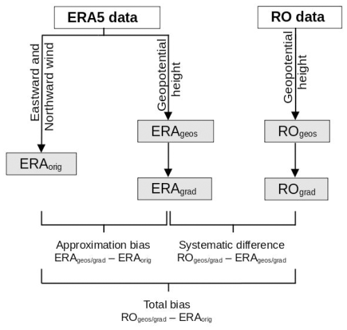
Figure 1 Schematic diagram of the three-step evaluation method. The original ERA5 (ERA_orig) wind speed is calculated based on the northward and eastward wind components. In the first step, geostrophic ERA5 (ERA_geos) and geostrophic RO (RO_geos) winds are estimated from the corresponding geopotential height data. In the second step, ERA5 gradient (ERA_grad) and RO gradient (RO_grad) winds are calculated using the previously derived ERA_geos and RO_geos values, respectively. The approximation bias is computed as the difference between the estimated ERA_geos and ERA_grad relative to ERA_orig, while the datasets' systematic difference is computed as the difference in the corresponding wind fields, ERA_geos and RO_geos or ERA_grad and RO_grad, respectively. The total bias is computed as the difference between estimated RO winds and ERA_orig.

For inspecting horizontal latitude–longitude maps, we concentrated on the four representative levels of 200, 150, 50 and 10 hPa, which represent the upper-troposphere, tropopause, lower-stratosphere and middle-stratosphere regions, respectively. As a focus region, we examined latitudinal–altitudinal cross-sections of the respective wind speed differences averaged over the 140–160° E longitudinal area. This longitudinal region was selected since the larger differences observed were mainly found there (i.e. roughly jet-stream core region). To assess the added value of RO data compared to ERA5 in terms of their temporal homogeneity and long-term stability, we analyse temporal differences in wind derived from the two datasets.

To derive wind fields, one commonly starts with the equations of zonal and meridional momentum (Holton and Hakim, 2013). However, due to the complexity of solving these non-linear partial differential equations, some assumptions and simplifications are useful to estimate approximate wind components. To derive them in line with the focus of this study from thermodynamic data (such as provided by RO), we first use the geostrophic approximation. In this approximation, most of the horizontal momentum equation terms are neglected, except for the Coriolis force term, which is balanced by the pressure gradient force. In the isobaric coordinate system, zonal (u_geos) and meridional (v_geos) geostrophic wind components are given by the following relations (Holton and Hakim, 2013; Scherllin-Pirscher et al., 2014; Verkhoglyadova et al., 2014):

$$\begin{array}{}\text{(1)}& {\displaystyle }{u}_{\text{geos}}={\displaystyle \frac{-\mathrm{1}}{f\left(\mathit{\phi }\right)a}}{\displaystyle \frac{\partial \mathrm{\Phi }}{\partial \mathit{\phi }}},\text{(2)}& {\displaystyle }{v}_{\text{geos}}={\displaystyle \frac{\mathrm{1}}{f\left(\mathit{\phi }\right)\mathrm{acos}\left(\mathit{\phi }\right)}}{\displaystyle \frac{\partial \mathrm{\Phi }}{\partial \mathit{\lambda }}},\end{array}$$

where f(φ) is the local Coriolis parameter, f(φ)=2Ωsin φ, with $\mathrm{\Omega }=\mathrm{7.2921}\times {\mathrm{10}}^{-\mathrm{5}}$; a is the Earth's radius; Φ denotes geopotential on isobaric levels; and φ is geographic latitude and λ longitude. Geopotential Φ is calculated as Φ=Zg₀, where Z is geopotential height and g₀=9.80665 m s⁻² is the standard gravity constant. Hence, to derive geostrophic wind fields, we need geopotential height fields at pressure levels as information. As shown in Scherllin-Pirscher et al. (2017), the geostrophic wind could also alternatively be derived as the gradient vector of the Montgomery potential at potential temperature surfaces, but the results do not differ from the geopotential-based derivation used here.

Based on the estimated geostrophic wind speeds, the gradient wind approximation is used. In this approximation, the pressure gradient term is balanced not only by the Coriolis force but by the Coriolis and the centrifugal force together. The equations for zonal (u_grad) and meridional (v_grad) gradient wind components are hence functions involving the geostrophic wind components as their backbone, calculated as (Holton and Hakim, 2013; Scherllin-Pirscher et al., 2014)

$$\begin{array}{}\text{(3)}& {\displaystyle }\begin{array}{rl}{u}_{\text{grad}}& =F\left(u_{\text{geos}},\mathit{\phi }\right)\\ & ={\displaystyle \frac{-f\left(\mathit{\phi }\right)\pm \sqrt{f^{\mathrm{2}}\left(\mathit{\phi }\right)+\mathrm{4}f\left(\mathit{\phi }\right)u_{\text{geos}}\tan \left(\mathit{\phi }\right)/a}}{\mathrm{2}\tan \left(\mathit{\phi }\right)/a}},\end{array}\text{(4)}& {\displaystyle }{v}_{\text{grad}}=F\left(v_{\text{geos}},u_{\text{grad}},\mathit{\phi }\right)={\displaystyle \frac{v_{\text{geos}}f\left(\mathit{\phi }\right)}{f\left(\mathit{\phi }\right)+u_{\text{grad}}\tan \left(\mathit{\phi }\right)/a}}.\end{array}$$

Here the ± sign refers to Northern Hemisphere (+) and Southern Hemisphere (−), respectively. The total wind speed is calculated as the square root of the sum of the squared zonal and meridional wind components, and we term this V_orig for the original wind, V_geos for the geostrophic wind and V_grad for the gradient wind.

This procedure was applied to both ERA5 and RO geopotential fields to estimate corresponding geostrophic winds and gradient winds. To assess the added value of the gradient wind approximation on top of the geostrophic approximation, we estimate the gradient wind delta-difference field ΔV defined as

$$\begin{array}{}\text{(5)}& \begin{array}{rl}\mathrm{\Delta }V& =\left|{\text{Bias}}_{\text{geos}}\right|-\left|{\text{Bias}}_{\text{grad}}\right|\\ & =\left|V_{\text{geos}}-V_{\text{orig}}\right|-\left|V_{\text{grad}}-V_{\text{orig}}\right|,\end{array}\end{array}$$

$$\begin{array}{c}{\displaystyle }\mathrm{\Delta }V>\mathrm{0}\to \left|{\text{Bias}}_{\text{grad}}\right|<\left|{\text{Bias}}_{\text{geos}}\right|,\\ {\displaystyle }\mathrm{\Delta }V<\mathrm{0}\to \left|{\text{Bias}}_{\text{geos}}\right|<\left|{\text{Bias}}_{\text{grad}}\right|.\end{array}$$

In using this convenient absolute delta-difference metric for inspecting the additional bias reduction or bias increase by the gradient wind approximation vs. the geostrophic approximation, the regions where both approximations give similar values will be suppressed (delta difference near zero), while areas with larger delta differences will stand out. Positive delta-difference values indicate better estimation of the original wind by the gradient wind approximation, while negative delta-difference values represent the opposite – better representation of the original wind by the geostrophic approximation.

Since deriving geostrophic wind fields is based on the horizontal derivatives of geopotential height, it is desirable for the geopotential height field to be smooth. As the ERA5 geopotential field is derived by numerical integration, it is smoother compared to the observation-based RO geopotential field. Hence, we smoothed the 2.5° × 2.5° RO geopotential fields using a five-point Gaussian filter in the longitudinal and latitudinal direction. In the latitudinal direction, the last two latitude circle grid lines were excluded from the analysis, since they are needed as a filter margin. Additionally, one more grid line (85°) was discarded after calculating the derivative according to Eq. (1). The final latitudinal range used for the RO-derived fields is ±82.5°. Related to this, due to the lower number of soundings over the polar caps (as well as the complexity of calculations over polar regions), it is justified to exclude these few polar latitude circles from the analysis in both RO and ERA5 wind fields.

Such filtering smoothes not only the noise component, but also part of the signal. Hence the spatial resolution of the field decreases (Vishwakarma et al., 2018). The amplitude of the damped signal depends on the type of filter selected. For a Gaussian filter, the resulting resolution of the fields gets coarser by a factor of 2 compared to the smoothing radius (Devaraju, 2015). Overall, it is clear that there are differences in the spatio-temporal representation of ERA5 and RO data. Regarding the temporal component, we can assume that temporal weighting applied to the daily RO profiles does not strongly influence the monthly-mean value. On the other hand, ERA5 (and ECMWF IFS model) winds are also filtered by spatial and temporal diffusion operators (Hersbach et al., 2020). In summary, these post-processing methods affect the physical spatial resolution of the field. To estimate the effective physical resolution of the resulting climatic field is hence not an easy task (e.g. Vishwakarma et al., 2018). We plan to investigate this aspect more thoroughly in our future research by testing various filtering options and inspecting their influence on wind fields over mountainous regions, where fine horizontal structures are usually observed.

As the Coriolis parameter f(φ) approaches zero near the Equator, the approximations are not valid in those areas. A separate wind analysis based on the thermal wind balance was carried out by Danzer et al. (2024) for the equatorial region. Still, because in our data grids the lowest-latitude bin grid lines are at ±1.25° latitude, it was possible to calculate winds for all climatological bins, though values close to the Equator lose physical meaning. In this way we determined the region of approximation breakdown by comparing the approximation bias to some commonly used accuracy requirement values.

We used the monthly-mean geopotential data at isobaric levels for the January and July months in the period 2007–2020 to derive the geostrophic wind components using Eqs. (1) and (2) and gradient winds using Eqs. (3) and (4), and we subsequently computed the speed as the magnitude of the corresponding wind vector. The wind speeds for ERA_orig, ERA_geos, RO_geos, ERA_grad and RO_grad were then used to perform our evaluations according to Fig. 1. All calculations, the statistical analysis and the visualisation were performed using the Python programming language, mainly its packages NumPy, Xarray, pyMannKendall and Matplotlib.

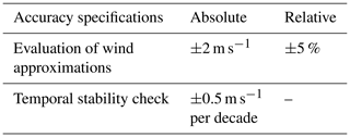
To put the results into context with reasonable wind accuracy requirements (e.g. Stoffelen et al., 2020), we used absolute requirement values for domains with low wind speeds, while for high wind speeds, relative requirement values appear a more appropriate choice. We chose a difference of ±2 m s⁻¹ or a relative difference of ±5 % as requirements, which are values consistent with the wind observation accuracy target requirements specified by the World Meteorological Organization (WMO) for various applications, including NWP and climate (Stoffelen et al., 2020; WMO-OSCAR, 2022; Table 1). Simple linear regression was used to test the long-term temporal stability of the derived wind speed fields. We estimated the decadal trend rate of the difference between RO_geos and ERA_geos and evaluated this against the WMO-GCOS (2016) wind measurement stability target requirement of ±0.5 m s⁻¹ per decade (see also Table 1).

Table 1 Selected absolute and relative wind speed accuracy requirements used in the study, informed by WMO-GCOS (2016).

3 Results

3.1 Approximation bias – ERA_geos and ERA_grad vs. ERA_orig

To test the strengths and weaknesses of the geostrophic and gradient wind approximations, we compare estimated ERA_geos and ERA_grad to the original ERA_orig winds for January (Fig. 2) and July (Fig. 3). We show the ageostrophic contribution as a reference bias field, while for gradient wind we present delta differences calculated based on Eq. (5). This delta-difference approach allows us to show only regions where gradient wind approximation estimates original wind notably better (i.e. positive delta-difference values) or notably worse (i.e. negative delta-difference values) compared to the geostrophic balance. Hence, where the delta difference is small, the approximations give relatively similar wind estimations.

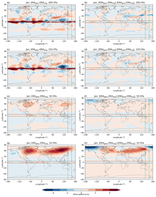
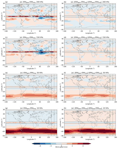
Figure 2 Long-term (2007–2020) mean approximation bias. Wind speed differences (m s⁻¹) between the geostrophic ERA5 (ERA_geos) and the original ERA5 (ERA_orig) wind (left column), and the gradient wind (ERA_grad) delta difference calculated using Eq. (5) (right column), at the 200 hPa (a, b), 150 hPa (c, d), 50 hPa (e, f) and 10 hPa (g, h) levels for January. Dashed green vertical lines denote the 140–160° E area for which vertical cross-sections are given (see Fig. 4). Dashed black horizontal lines delineate the ±5° latitude band around the Equator and ±82.5° regions towards the poles.

Figure 3 The same as Fig. 2 but for July.

For both approximations some of the same deviations from the original wind are observed in the regions where the centrifugal term does not contribute much (i.e. in equatorial and tropical regions). At two lower selected levels and in both seasons, the largest amplitude of the differences is found around the Equator from −5 to 5° latitude as a result of the Coriolis parameter approaching zero. These differences are clearly larger than the selected accuracy threshold of 2 m s⁻¹, indicating the region of approximation breakdown. At lower levels, larger underestimation of original wind is observed in monsoonal regions over Indonesia in January and the tropical Indian Ocean in July (Figs. 2c, 3c). Larger positive biases (up to 6 m s⁻¹) are observed in the subtropical jet stream over the winter hemisphere. At the lowest 200 hPa level, a glimpse of stationary waves is noticeable as a dipole structure above the western part of North America, as well as a dipole over SW Asia (Fig. 2a).

The largest differences between the geostrophic and the gradient wind approximations are present at the lowest 200 hPa (Figs. 2a–b, 3a–b) and at the highest 10 hPa (Figs. 2g–h, 3g–h) observed levels. The geostrophic balance describes the original wind better at the lower levels, especially over the Pacific Ocean in the regions of the subtropical jet-stream core where gradient wind approximation underestimates the original wind (∼ ±30° lat) (Figs. 2a and 3a). On the other hand, the gradient wind performs better in the lower-stratosphere and mid-stratosphere regions, specifically in depicting the stratospheric polar night jet (∼ ±60° lat) (Figs. 2h and 3h). The gradient wind balance works better for July stratospheric winds, unlike in January, when it significantly underestimates wind in the northernmost polar regions.

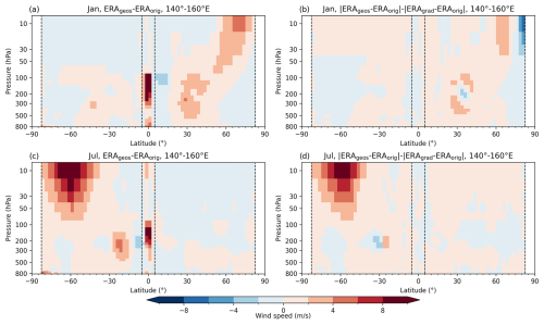
Figure 4 Long-term (2007–2020) mean vertical cross-section of the approximation bias. Wind speed differences (m s⁻¹) between the geostrophic ERA5 (ERA_geos) and the original ERA5 (ERA_orig) wind (a, c) and the gradient wind (ERA_grad) delta difference calculated using Eq. (5) (b, d), averaged over the 140–160° E area for January (a, b) and July (c, d). Dashed black vertical lines delineate the ±5° latitude band around the Equator and ±82.5° regions towards the poles.

To better understand the altitudinal–latitudinal behaviour of both approximation biases, we examine its latitudinal vertical cross-section averaged over the region 140–160° E (Fig. 4). This longitudinal region is selected because both larger deviations from the subtropical jet stream and polar night jet are found here (i.e. region of strengths and weaknesses of geostrophic and gradient wind approximation). In both seasons, both approximations are not valid in the equatorial region between ±5° latitude. Generally, the geostrophic approximation is better in describing the dynamics of the subtropical jet stream, while the gradient wind approximation works better at higher levels since the delta difference is positive there, especially during Southern Hemisphere (SH) winter. An underestimation of the Northern Hemisphere (NH) stratospheric polar jet stream by the gradient wind approximation is noticeable through negative delta-difference values in the high-latitude regions (Fig. 4b). Except for the larger deviations in describing subtropical jet stream or polar night jet mentioned, wind speed differences are well within the accuracy requirement of 2 m s⁻¹.

3.2 Systematic difference – RO_geos/grad vs. ERA_geos/grad

In line with the second study goal, we tested how well RO-derived and estimated ERA5 wind fields agree, applying the same approximation to both data products. Building upon the results from Sect. 3.1, the equatorial band within ±5° is excluded from further inspection. We focus on understanding the consistency between RO- and ERA5-estimated wind speed in those (still) nearly global domains, where the approximations are found to perform well. Since this systematic difference between the two datasets (RO vs. ERA5) is equal for geostrophic and gradient wind, for convenience we show the results only for geostrophic wind.

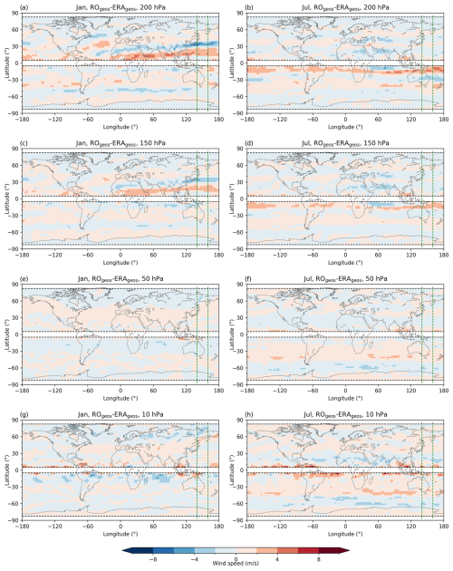
Figure 5 Long-term (2007–2020) mean systematic difference between RO and ERA5. Wind speed differences (m s⁻¹) between the geostrophic RO (RO_geos) and the geostrophic ERA5 (ERA_geos) wind at 200 hPa (a, b), 150 hPa (c, d), 50 hPa (e, f) and 10 hPa (g, h), for January (left column) and July (right column). Dashed green vertical lines denote the 140–160° E area for which vertical cross-sections are given (see Fig. 6). Dashed black vertical lines delineate the ±5° latitude band around the Equator and ±82.5° regions towards the poles.

An inspection of the differences in horizontal maps at four selected levels reveals that the overall wind patterns are well represented by the RO wind data (Fig. 5). Generally, the differences are larger over the winter hemisphere, especially in the region of the subtropical jet stream at 200 hPa where RO_geos over-/underestimates ERA_geos at around ±20/30° latitude (Fig. 5a, b). Such a pattern might indicate that, based on the geopotential data, the position of the jet stream is moved slightly further equatorward in the RO data compared to the ERA5 dataset. This difference is still present at the 150 hPa level but with lower amplitudes (Fig. 5c, d). At 50 hPa, differences are well within ±2 m s⁻¹ (Fig. 5e, f). In both seasons at the highest level of 10 hPa, differences of up to 4 m s⁻¹ are found in the tropical region (Fig. 5g, h).

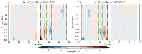
Figure 6 Long-term (2007–2020) mean vertical cross-section of the systematic difference between RO and ERA5. Wind speed differences (m s⁻¹) between the geostrophic RO (RO_geos) and the geostrophic ERA5 (ERA_geos) wind, averaged over the 140–160° E area for January (a) and July (b). Dashed green vertical lines denote latitudinal belts used in the further analysis of long-term temporal consistency of the datasets. Dashed black vertical lines delineate the ±5° latitude band around the Equator and ±82.5° regions towards the poles.

Investigating the latitudinal cross-section confirms that the larger differences observed (up to around 6 m s⁻¹) in the winter hemisphere correspond to the locations of the subtropical jet stream (Fig. 6). A maximum January amplitude, showing a positive difference at ∼ 300 hPa and a negative one at ∼ 200 hPa, might also point to a somewhat lower location of the jet-stream core in RO data compared to the ERA5 data (Fig. 6a). In July, such a difference in the location of the jet-stream core between the two datasets is not noticeable (Fig. 6b).

To better understand these systematic differences, we investigate latitudinal and altitudinal temporal variations over the longitude sector of 140–160° E. This longitude sector was selected because the subtropical jet stream seems to leave a quite distinct feature over the western Pacific; differences of up to ±6 m s⁻¹ (i.e. up to and exceeding the Table 1 threshold requirements) are seen in this sector in the winter hemisphere (see Fig. 5a, b).

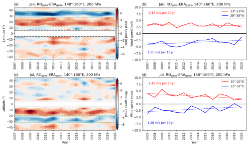
Figure 7 Latitudinal temporal distribution of the systematic difference between RO and ERA5. Wind speed difference (m s⁻¹) between the geostrophic RO (RO_geos) and the geostrophic ERA5 (ERA_geos) wind, averaged over the 140–160° E area at 200 hPa (a, c) for January (a) and July (c). Dashed green horizontal lines denote 10° latitudinal belts of 13–23 and 28–38° N in January and 10–20 and 22–32° S in July, for which the temporal trend analysis is made (b, January; d, July; Table 2). Dashed black horizontal lines delineate the ±5° Equator band.

A 2007–2020 temporal analysis (Fig. 7) reveals that this pattern is systematic, with belts of positive and negative differences within 10 to 40° latitude in the winter hemisphere (Fig. 7a, c). We therefore further define equally wide latitudinal belts that encompass the over- and underestimations discussed to estimate the value of temporal change. For January, we define the regions of RO-derived wind over-/underestimation within the latitudinal belt of 13–23/28–38° N, while for July the belt is 10–20/22–32° S. The time-series analysis revealed that both the positive and the negative differences between the two datasets decrease with time (Fig. 7b, d). Exceedance of the WMO-GCOS target requirement (Table 1) for long-term stability within ±0.5 m s⁻¹ per decade, taken as a consistency benchmark, is detected at the 200 hPa level in both seasons for negative differences and in July for positive differences as well (Fig. 7b, d). However, when calculated at other levels, e.g. 300 hPa or 250 hPa, the bias in the region of RO wind overestimation is below the ±0.5 m s⁻¹ threshold in January (Table 2).

Table 2 Decadal trend values (m s⁻¹ per decade) in the systematic difference between the geostrophic RO and the geostrophic ERA5 wind speeds, averaged over the 140–160° E longitudinal area and in latitudinal regions of 13–23 and 28–38° N in January and 10–20 and 22–32° S in July at the 200, 250 and 300 hPa levels. Systematic-difference trend rates larger than the WMO-GCOS (2016) long-term stability requirement of ±0.5 m s⁻¹ per decade (Table 1) are in bold.

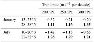
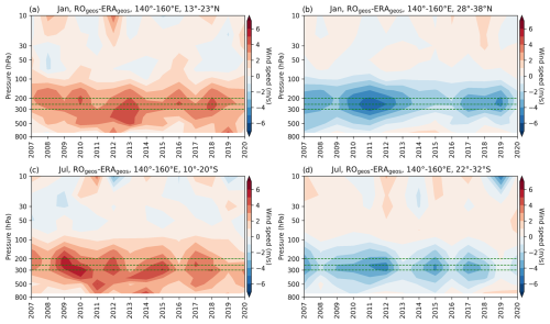
Figure 8 Altitudinal temporal distribution of the systematic difference between RO and ERA5. Wind speed difference (m s⁻¹) between the geostrophic RO (RO_geos) and the geostrophic ERA5 (ERA_geos) wind, averaged over the 140–160° E area for (a) 13–23° N and (b) 28–38° N in January and (c) 10–20° S and (d) 22–32° S in July. Dashed green lines denote the 200, 250 and 300 hPa levels for which the decadal trend values are given in the Table 2.

The explanation of this result is shown in the Fig. 8. Besides the temporal change in its amplitude, we also find an altitudinal shift in the systematic difference. This is more expressed for belts where RO_geos overestimates ERA_geos wind. From that, we can conclude that an analysis of changes in the jet-stream core position based on ERA5 and RO data can give somewhat different results. Such detected temporal and altitudinal differences in the systematic bias might correspond to major observing system changes in the ERA5 data assimilation (Hersbach et al., 2020, Figs. 3 and 4 therein).

3.3 Total bias – RO_geos/grad vs. ERA_orig

In the final step, we show the total wind speed bias, i.e. how well the original ERA5 wind field is estimated by RO-derived winds. Here, we evaluate the total wind speed bias in regard to WMO-related requirements (Table 1).

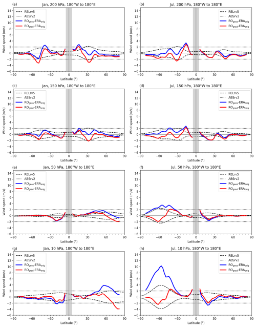
Figure 9 Latitudinal distribution of the total bias. Wind speed difference (m s⁻¹) between the geostrophic RO (RO_geos) and the original ERA5 (ERA_orig) wind (blue line) and between the RO gradient (RO_grad) and the original ERA5 (ERA_orig) wind (red line) at the 200 hPa (a, b), 150 hPa (c, d), 50 hPa (e, f) and 10 hPa (g, h) levels for January (left column) and July (right column). WMO-based accuracy requirement values are indicated in absolute terms at values of 2 m s⁻¹ (ABSrv2, dotted black line) and in relative terms at 5 %, with reference to the original ERA5 wind speed (RELrv5, dashed black line).

At the lowest observed level (200 hPa), in both seasons RO_geos gives better estimates of ERA_orig compared to RO_grad. For RO_geos these differences are generally below 2 m s⁻¹, except for the slight overestimation (∼ 3 m s⁻¹) at ∼ 15° winter hemisphere latitude (Fig. 9a–b). Generally good agreement of RO_geos and ERA_orig is also observed at the 150 hPa level, with a slightly lower overestimation at ∼ 15° winter hemisphere latitude (Fig. 9c–d). At the 50 hPa level, both approximations give January wind estimations with bias below 2 m s⁻¹, while in July RO_geos overestimates ERA_orig wind at ∼ 60° S by around 4 m s⁻¹ (Fig. 9e–f). At the highest selected level (10 hPa), RO_geos overestimates ERA_orig for around 4 m s⁻¹ at 60° N, while RO_grad underestimates it by ∼ 4 m s⁻¹ in high-latitude polar regions (Fig. 9g). On the other hand, in July, RO_geos overestimation over the Southern Hemisphere is larger than 10 m s⁻¹, while RO_grad gives estimates with accuracy within 2 m s⁻¹ (Fig. 9h).

Hence, in the last step we show horizontal fields of the total bias between RO-derived and original ERA5 wind at selected levels, where we show RO_geos wind for the two lower levels and RO_grad wind in the upper two levels.

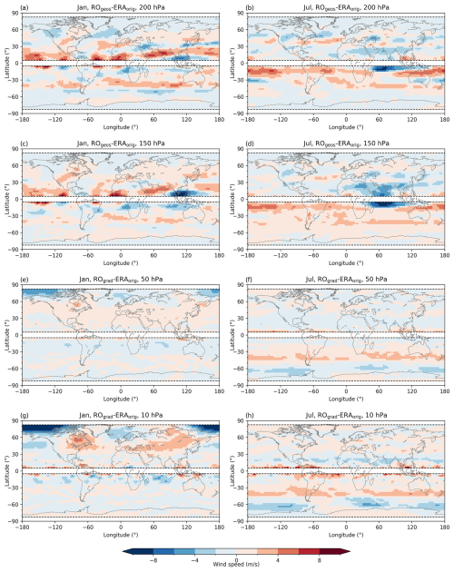
Figure 10 Long-term (2007–2020) mean total bias. Wind speed differences (m s⁻¹) between the geostrophic RO (RO_geos) and the original ERA5 (ERA_orig) wind at the 200 hPa (a, b) and 150 hPa (c, d) levels and between the RO gradient (RO_grad) and the original ERA5 (ERA_orig) wind at the 50 hPa (e, f) and 10 hPa (g, h) levels for January (left column) and July (right column). Dashed black horizontal lines delineate the ±5° latitude band around the Equator and ±82.5° regions towards the poles.

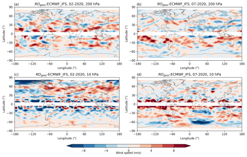
Based on the results shown in the previous sections, it is clear that the total bias in the subtropical jet stream is a result of the systematic difference and the approximation bias (Fig. 10a–b). On the other hand, a larger underestimation of winds by RO_geos in the monsoonal region, as well as dipole structures related to stationary waves, is mainly a result of the inability of the geostrophic approximation to capture such a circulation (Fig. 10c–d). Similar patterns can be seen in Fig. A1a–b, where a comparison between geostrophic RO wind speeds and ECMWF IFS analysis wind speeds at 200 hPa for February and July 2020 is shown as complementary information. However, as to be expected, the Fig. A1 differences exhibit more details and a larger spatial variability compared to Fig. 10, where variability is lower due to the temporal averaging.

In the upper levels, the total bias is mainly the result of the applied approximation (Fig. 10e–h). The exception is the tropical region, where lower RO data quality contributes to somewhat larger bias. The NH high-latitude RO_grad wind underestimation in January is caused by neglecting the horizontal advection terms, which are important during condition when strong wave activity and the polar night jet interact. Again, the robustness of the results is supported by a further complementary comparison with two test months of ECMWF IFS analysis data (Appendix, Fig. A1c–d). Similar patterns are observed, with more strongly expressed noise-like differences near the Equator.

4 Discussion

The main goal of this study was to test the general ability of RO-derived climatic winds to represent original ERA5 winds on a 2.5° × 2.5° horizontal grid. For this purpose, we decomposed the total wind speed bias into the contribution depending on the approximation method (approximation bias) and the contribution from the difference between the two datasets (systematic difference).

First, the ability of conventionally used local force balance approximations, geostrophic and gradient wind balance, to represent original monthly-mean wind speeds was evaluated based on the ERA5 data. The validation was performed horizontally (from Equator up to ±82.5° and from 180° W to 180° E) and vertically (from the bottom of the free troposphere at 800 hPa up to the middle stratosphere at 10 hPa). Testing commonly used methods to estimate wind speed based on the thermodynamic data showed that, regarding the limitations of the Coriolis parameter as one approaches the Equator, in the free troposphere it is possible to use approximations up to ±5° latitude. In the stratosphere it was possible to derive winds from the approximation towards ±2.5° latitude. However, since we focus on the long-term mean wind speed bias, an overestimation in the zonal/meridional wind component joint with a possible underestimation of the meridional/zonal component might result in a low total wind speed bias. This result is also supported by findings in Danzer et al. (2024). They comment that the breakdown of the geostrophic balance is mainly related to a larger bias in the meridional component. This is why in the stratosphere, where tropical flow is dominantly zonal, the approximation bias is lower.

Even though the gradient wind approximation is a generalisation of the geostrophic balance, it does not imply that it will always give the better estimation of the real wind. In accordance with earlier studies, the geostrophic approximation is a suitable method to describe a wind field in the free troposphere (Boville, 1987; Scherllin-Pirscher et al., 2014; Verkhoglyadova et al., 2014). We detected the dominant ageostrophic features in the area of the subtropical jet stream and monsoonal region in the winter hemisphere, as well as above large mountain ranges in winter. The dipole patterns above mountains are related to the stationary waves which are quite common in the NH winter mid-latitudes. Still, due to long-term averaging, they are not as expressed as in Fig. 2 in the study of Scherllin-Pirscher et al. (2014). Such features arise from the zonal differences in the topography, land–sea distribution and atmospheric diabatic heating. Their structure and magnitude depend on the characteristics of the jet stream (Wills et al., 2019). Accordingly, long-term averaging might damp such features in regions where their inter-annual variability is larger. However, dipole structures related to the impact of the Rocky Mountains and Himalaya on the large-scale wind flow (e.g. Sandu et al., 2019) are present in the long-term ageostrophic term. Hence, not accounting for advection terms in the momentum equations fails to correctly reproduce these wave–mean flow interactions. On the other hand, thermally driven monsoonal circulation shows small inter-annual variations in its direction and position, so its contribution to the ageostrophy is also well expressed in the long-term mean. Again, neglecting horizontal advection of momentum resulted in typical upper-air monsoonal winds not being well captured, with the strongest bias at around 150 hPa (Trenberth et al., 2000).

On the other hand, a larger contribution of curvature effects, as well as of very strong winds, enables a better stratospheric wind field estimation (especially over the mid-latitudes) using the gradient wind approximation (Elson, 1986; Boville, 1987; Randel, 1987). Significant geostrophic wind overestimation in these regions is reduced by retaining the centrifugal term in the equations of motion. Even though the SH winter polar night jet is well described using the balanced gradient winds, this is not the case for the NH, where the winter polar night jet is more asymmetrical. Larger underestimation of the original wind by the gradient wind balance is detected in high-latitude regions at ∼ 80° N, which has also been found in other papers (Elson, 1986; Randel, 1987). This is due to the effect of the Aleutian High in those regions, a high-pressure system commonly found in the NH stratosphere during the winter season (Colucci and Ehrmann, 2018; Elson, 1986; Harvey and Hitchman, 1996). By omitting horizontal advection terms (i.e. wave flux terms), the effect of this pressure system on the polar night jet in this region is not well included, resulting in the underestimation of the original wind by the gradient wind balance. Overall, both methods capture general features of global climatic winds on a synoptic scale, from the free troposphere to the mid-stratosphere, excluding the equatorial region.

The successful performance of the methods is of great importance for enabling reliable long-term dynamical wind field monitoring based on the thermodynamic mass field data, such as those available in the form of RO-derived isobaric geopotential height data. Hence, in a second step, we tested how well RO-derived climatic winds agree with the corresponding ones estimated from ERA5 data. Here, we additionally test the temporal changes in this systematic difference to check for possible inhomogeneities. The analysis of the systematic differences between ERA5 and RO datasets revealed generally good agreement over the whole near-global free-troposphere–mid-stratosphere domain. The largest differences are observed in the region of the subtropical jet-stream core. The systematic differences are larger in the lower levels compared to the upper ones. Even though the geopotential difference between the two datasets is quite small (here not shown), compared to the magnitude of the geopotential itself (below 1 %), we find that such small differences can lead to appreciable differences in wind speeds (up to 8 m s⁻¹), since these derive from the spatial derivatives of the isobaric geopotential fields.

A systematic underestimation in the centre of the subtropical jet stream and an overestimation in its equatorward parts indicate a difference in the subtropical jet-stream position between the two datasets. Mentioned deviations in the subtropical jet stream are analysed in detail by testing its long-term stability using linear trend fits over 2007–2020. We estimated a trend magnitude of more than 0.5 m s⁻¹ per decade, which exceeds the WMO-GCOS (2016) long-term stability requirement. Besides temporal changes in the amplitude of the systematic difference, temporal differences in altitudinal direction are also observed. Since RO data are shown to be stable in the long term (Steiner et al., 2020a), such findings might point to the effect of changes in the assimilated data in ERA5 (Hersbach et al., 2020). This result indicates the potential advantage of RO-derived winds in terms of long-term stability for multi-decadal wind field monitoring, for example, to monitor the changes in large-scale circulation patterns such as the tropical–subtropical Hadley circulation (e.g. Weatherhead et al., 2018) or in the subtropical and polar jet streams.

Generally, the approximation bias and the systematic difference are both larger in the winter hemisphere, where the atmosphere is more dynamic in terms of higher wind speeds and stronger wave activity (Wu and Jehn 1972; Scherllin-Pirscher et al., 2014, 2017; Verkhoglyadova et al., 2014). This is one of the reasons why early validation studies a few decades ago were mainly performed for the winter season, especially over the NH, as wave activity is then more expressed (e.g. Elson, 1986; Boville, 1987; Randel, 1987).

This study advances on earlier initial studies to derive wind fields based on RO data (Scherllin-Pirscher et al., 2014, 2017; Verkhoglyadova et al., 2014). One of the advances is our twofold approach, where we decompose the total wind bias into a contribution from the wind approximation bias and another part derived from the systematic difference between the datasets. Scherllin-Pirscher et al. (2014) commented that the total wind bias is mainly caused by the wind approximation used, rather than the effect of RO retrieval errors. However, here we show that in the free-troposphere region, the systematic difference between the two datasets in the subtropical jet-stream region also contributes to the total bias. The finer horizontal grid used here (2.5°) compared to those of previous studies (5°) allowed us to go more equatorward to reliably explore the region of the breakdown of the geostrophic approximation. While previous studies excluded the tropical regions between ±10° or ±15° (based on the argument of the Coriolis force becoming small), we found that it is reliably possible to only exclude the ±5° equatorial band in the free troposphere and ±2.5° band in the lower stratosphere. In addition, compared to the earlier studies, where a few specific years were selected for the initial analyses, here we analysed long-term wind speed means, including the decadal-scale temporal stability, which gave more robust results.

5 Conclusions and perspectives

The investigation of the appropriate approximation method to derive winds, combined with the suitability of RO data for estimating climatic winds based on the geopotential fields, gave generally encouraging results.

Our main findings include the following:

• Regarding the singularity of the Coriolis parameter near the Equator, with the applied spatial grid of 2.5° latitude × 2.5° longitude, it is possible to use geostrophic/gradient wind approximations equatorward as close as down to 5° latitude in the free troposphere and 2.5° latitude in the lower-stratosphere region.

• It is justified to use the geostrophic approximation as a method to estimate winds in the free troposphere, while for the stratospheric winds, the additional inclusion of the centrifugal term contributes to better wind estimation.

• In the free troposphere, larger ageostrophic contributions are found in the subtropical jet-stream region, over large mountain ranges and in the monsoon regions due to neglecting the horizontal advection terms and/or vertical wind component in the equations of motion.

• In the stratosphere, the largest bias of the gradient wind approximation is detected in NH polar regions, where the effect of wave–polar night jet interaction is not included due to neglecting horizontal advection terms in the equations of motion.

• The differences between RO and ERA5 geostrophic winds are generally small with values well within ±2 m s⁻¹, except in the region of the subtropical jet stream, where patterns of latitudinal over- and underestimation are observed, pointing to possible differences in the jet-stream position between the two datasets.

• Trend analysis of the detected jet-stream difference showed an exceedance of the WMO-GCOS (2016) 0.5 m s⁻¹ per decade stability requirement, pointing to an inhomogeneity in ERA5 data due to observing system changes and potential added value from the long-term stability of RO-derived wind field records.

• Overall, the total difference between RO-derived wind (geostrophic wind in the free troposphere and gradient wind in the stratosphere) and original ERA5 wind is small in monthly-mean wind fields, with differences in the troposphere due to both approximation bias and the systematic difference between the datasets and differences in the stratosphere due to the approximation bias.

Despite this decent progress towards assessing the utility of RO records for wind monitoring, some problems and questions remain. One future goal is to create a global climatic wind speed dataset based on RO data. For these purposes the equatorial region between ±5° latitude, which was excluded here, needs to be filled. Healy et al. (2020) showed that RO-derived zonal-mean-balance winds quantify stratospheric zonal winds at the Equator well. However, this equatorial-balance-approximation approach did not provide information on geographically gridded wind fields and appears to lack information on lower altitudes into the free troposphere. Following Healy et al. (2020) and Scaife et al. (2000), Danzer et al. (2024) went a step further and derived wind fields in tropical regions using the equatorial balance approximation. They also showed that the geostrophic approximation works well in estimating zonal-mean zonal wind in this region, while larger deviations are observed for the meridional wind component.

Hence, it is needed to combine these RO-estimated wind fields based on three different methods (equatorial wind balance in the tropics, geostrophic wind in the troposphere and gradient wind in the stratosphere) to derive a physically meaningful wind field dataset. Additional improvements in approximation methods are needed in the regions where advection terms were shown to be important (e.g. NH winter mid-latitudes and the monsoon region in the free troposphere as well as the stratospheric NH near-polar region). For these purposes, we plan to adapt and validate the methods proposed by Elson (1986) and Randel (1987).

Another avenue is the already-mentioned lower accuracy of RO data above about 30 km, mainly related to residual ionospheric biases. The potential of improving geopotential height data from RO at these altitudes does exist (e.g. Healy and Culverwell, 2015; Danzer et al., 2020, 2021; Liu et al., 2021; Syndergaard and Kirchengast, 2022), and the use of the most recently reprocessed RO data records is expected to also help improve wind monitoring in the upper stratosphere, allowing wind estimation up to the 5 hPa level. With improved RO data accuracy, RO climatic winds might provide additional information about the corresponding dynamics at these high altitudes. On the other hand, reanalysis assimilates fewer observational data towards higher altitudes (e.g. Podglajen et al., 2014), and the output is less observation-constrained and more strongly a result of the model used.

Overall, the added value of RO data is expected to be provided by its unique combination of fine vertical resolution, high accuracy and long-term stability over inter-annual to decadal time periods of climate change relevance. This capacity to accurately keep long-term consistency valuably complements the dense resolution and coverage qualities of reanalyses, where occasional inhomogeneities due to changes in observing systems are experienced. As stated in Hoffman et al. (2017), “It is imperative that researchers understand the sources, uncertainty, biases and other limitations of any data that they use”.

For reanalyses that is not an easy task due to the sources of uncertainties and errors arising from assimilated data, the numerical weather forecast model used and the assimilation method applied (Parker, 2016). In contrast, the uncertainties and errors in RO data are well understood and assessed (Steiner et al., 2020a). The potential for climate-related studies is manifold, and given the increasing observational database from the multi-satellite RO observing systems, RO climatic winds can serve as a valuable complementary data source for wind field monitoring and climate analyses.

Appendix A

Figure A1 Difference between RO climatic and ECMWF IFS wind speeds at the 200 hPa level (a, b) and 10 hPa level (c, d) for February 2020 (a, c) and July 2020 (b, d).