Satellite-based detection of deep-convective clouds: the sensitivity of infrared methods and implications for cloud climatology

Reliable deep-convective cloud (DCC) climatology relies heavily on accurate detection. Infrared-based algorithms play a critical role, as they are the only ones that can be applied to the 6.7 µm water vapour (WV) absorption band and the 11 µm infrared (IR) window band. For over 40 years, the latter has been the only daytime/nighttime channel used in satellite cloud imaging. This study presents the first global validation of three commonly used DCC detection methods, which use brightness temperature (T_b) in the WV and IR bands. These methods are the infrared-window method (IRW; T_b11), the brightness temperature difference method (BTD; T_b6.7−T_b11), and the temperature difference method with the tropopause method (TROPO; T_b11−T_tropo). All methods were applied to 1 year (2007) of Moderate Resolution Imaging Spectroradiometer (MODIS) observations and validated against collocated CloudSat-CALIPSO lidar–radar cloud classifications. Results indicate that even with optimal parameter configurations, DCC detection accuracy remains moderate and is below 75 % (Cohen's κ < 0.4) for all methods. Global accuracy ranged from 56.6 % (for TROPO) to 72.8 % (for BTD) using an optimal threshold of −2 K. Regionally, the BTD method performs best, with an accuracy of 72.9 % over Europe and 67.9 % over Africa. Misclassifications are common with cloud types such as nimbostratus and altostratus (single-layer cloud regimes) and cirrus and altostratus (multilayer cloud regimes). Overall, the BTD method slightly outperforms the others, while TROPO is the least effective. Our study highlighted the high sensitivity of these methods to threshold selection. Even a ±1 K change in the threshold resulted in a 10 %–40 % variance in DCC frequency. This finding is of particular importance for the construction of homogenous DCC datasets, whether they are global mosaics or time series spanning multiple generations of satellite instruments.

1 Introduction

Deep-convective clouds (DCCs) are formed through moist convection in the troposphere. DCC cloud top pressures may exceed ∼ 450–500 hPa, and clouds may reach the tropopause or even penetrate the lower stratosphere. Although they are the least-frequent cloud type on Earth (Sassen and Wang, 2008), DCCs are the focus of scientific concern due to their role in the hydrological cycle (Nesbitt et al., 2006); their atmospheric chemistry (Wang and Prinn, 2000); and their association with severe weather events that include heavy precipitation, damaging wind, hail, tornadoes, or downburst phenomena (Taszarek et al., 2020). According to the European Environment Agency (2024), economic losses related to extreme climate events amounted to EUR 738 billion in EU member states, and one-third of that was caused by severe storms.

With global warming, more energy is being held in the atmosphere, and troposphere dynamics are changing. In the midlatitudes, the Hadley circulation is weakening and expanding poleward (Ceppi and Hartmann, 2016; Lu et al., 2007), causing changes in the track and intensity of extratropical storms (Baatsen et al., 2015; Bender et al., 2012; Lehmann and Coumou, 2015). Consequently, convective processes are expected to intensify, and the frequency of DCC-related severe weather events may also increase (Aumann et al., 2008; Berthou et al., 2022). Identifying climate trends requires DCC time series that span at least 3 decades and a reliable reporting method.

The traditional (non-instrumental) approach to reporting is to observe the state of the weather visually (by a human observer) and to report DCC-related phenomena such as cumulonimbus clouds, hail, lightning, or thunder (Taszarek et al., 2019). However, the limits of human perception make the method subjective and inaccurate, and the spatial coverage is limited (Eastman and Warren, 2014). Alternative techniques rely on ground- or satellite-based remote sensing. An orbital perspective is especially important for efficient mapping of DCCs, notably through the use of imagers that provide frequent observations with global coverage.

Passive satellite imagers detect DCCs based on their radiative properties. In the thermal infrared window (8–14 µm), DCCs are among the coldest objects in the field of view. Consequently, brightness temperature (T_b) thresholds can be set to discriminate between DCCs and the warmer background (Doelling et al., 2004; Gong et al., 2018; Govaerts et al., 2018; Mu et al., 2017). However, the most important shortcoming of this method is that both DCCs and cirrus clouds are characterized by low T_b thresholds in the infrared window. As a result, detection can be ambiguous; for example, cirrus anvils associated with DCCs can be misclassified as convective clouds.

The T_b threshold can be also applied to the water vapour absorption band (5.5–8 µm). In these wavelengths, electromagnetic emissions leaving Earth are absorbed by water vapour in the atmosphere as the signal propagates upward, toward space. As a consequence, most radiance that is detected by a satellite originates in the upper atmosphere, including the highly elevated tops of DCCs (Ackerman, 1996; Ai et al., 2017). However, the difficulties with this method are similar to those that arise with the thermal infrared-window approach. Here, cirrus clouds pose a threat as well.

DCCs can also be detected using shortwave radiation (∼ 4 µm or less), a combination of shortwave and longwave bands, or geophysical parameters retrieved from multispectral radiances. One of the most widely adopted approaches is the algorithm implemented by the International Satellite Cloud Climatology Project (ISCCP; Rossow and Schiffer, 1999). The ISCCP characterizes clouds based on their optical depth (COT; cloud optical thickness) and the atmospheric pressure at the cloud top (CTP; cloud top pressure) – measurements are based on 10.5 µm brightness temperature, 0.65 µm reflectance, and radiative transfer modelling. As COT and CTP are continuous values, thresholds are applied to divide COT–CTP distributions into discrete classes. DCCs are identified when COT > 23 and CTP < 440 hPa.

A key shortcoming of the ISCCP classification and of other algorithms that exploit shortwave radiation is that they are limited to daytime conditions. Tracking the diurnal DCC cycle requires a method that relies solely on longwave infrared observations. The design of such an algorithm is closely linked to the technical specifications of the cloud imaging instrument. Most first-generation imaging sensors implemented as few as three spectral bands, two of which were dedicated to the infrared domain (Holmlund et al., 2021). The infrared-window (IR-window) channel and the water vapour (WV) absorption channel were typically centred at 11 and 6.5 µm, respectively. Advances in sensor technology have since made it possible to consider additional IR spectral channels, such as the ozone thermal absorption band at 9.7 µm (Jurkovic et al., 2015). However, the long history of the 11 and 6.5 µm bands makes them indispensable for climatology, as they are the only way to derive multidecadal DCC time series.

One of the main disadvantages of IR-based approaches is the need for a threshold: T_b (or the T_b difference) is used to discriminate between DCCs and non-DCCs. Historically, thresholds were set arbitrarily rather than being derived from an empirical examination (see Sect. 2.2 for details). Notably, DCC detections were not validated, and accuracy assessments were not reported (e.g. a classical confusion matrix for a binary classifier). The resulting DCC climatologies were only compared with other (independent) datasets to check for discrepancies among sources (Sarkar et al., 2022; Sassen and Wang, 2008). Such cross-comparisons cannot be considered a substitute for validation.

The primary reason for the lack of validation was the absence of a reliable ground truth. In cloud research there is no 100 % accurate dataset on cloud types, mostly due to the lack of a single unambiguous (i.e. method-independent) definition of cloud types. For instance, visual observers define DCCs by verbal description and the co-occurrence of DCC-associated weather phenomena. On the other hand, DCCs in the ISCCP project are defined by the physical parameters of the cloud: a certain optical thickness and tops above a certain height. As a consequence any validation of cloud type detection is in fact a relative comparison assuming that one source of observations is – for well-justified reasons – more reliable than the other dataset (i.e. the one being validated). Currently, the state-of-the-art data for validating cloud products originated from the CloudSat and Cloud–Aerosol Lidar and Infrared Pathfinder Satellite Observations (CALIPSO) missions. CloudSat hosted a cloud profiling radar, and CALIPSO hosted a cloud profiling lidar. Rather than imaging the horizontal distribution of cloud, lidar and radar provide a vertically resolved structure of the atmosphere. Due to this unique ability, clouds are classified both during the day and at night based on their horizontal extent, height, thickness, homogeneity, and the presence of precipitation rather than column-integrated radiances (Stephens et al., 2002; Winker et al., 2003). An important consideration is that CloudSat and CALIPSO were configured to fly in close formation with the Aqua satellite (Vincent and Salcedo, 2003), enabling quasi-simultaneous observation of clouds by lidar, radar, and Aqua's Moderate Resolution Spectroradiometer (MODIS) instrument (Barnes et al., 1998).

The CloudSat-CALIPSO cloud typing algorithm was introduced by Wang and Sassen (2001), and its accuracy has been demonstrated with surface-based lidar and radar observations. It was initially validated against visual (manual) cloud genera observations performed at the lidar–radar location and in accordance with the World Meteorological Organization standards. The validation study consisted of 540 cases, of which only 4 (according to reference data) or 9 (according to the lidar–radar classification) were DCCs. Wang and Sassen (2001) stated that the overall accuracy of their classification was 70 % but provided no specific details for DCCs.

Sassen and Wang (2008) ran a post-launch assessment of the classification. The authors focused on 1 full year of CloudSat observations (CALIPSO was excluded). Rather than performing a typical accuracy assessment, they only compared zonally averaged frequencies of individual cloud types. They found that the radar classification reported fewer DCCs than ISCCP or surface-based data did and reported more altostratus (As) and nimbostratus (Ns) clouds than the remaining databases. A similar study by Sarkar et al. (2022) noted that the difference between CloudSat-CALIPSO, ISCCP, and surface-based visual observations was highest for DCCs. These authors hypothesized that this difference may be related to the fuzzy logic used in the lidar–radar classification algorithm. Further validation studies of CloudSat data have considered specific geophysical parameters, notably cloud base height (Candlish et al., 2013), precipitation (Kodamana and Fletcher, 2021), or cloud phase (Wang et al., 2024), but not the cloud classification.

Despite limitations, CloudSat and CALIPSO data, especially when combined into one joint product, have been tested and adopted for validation purposes, including DCCs. Specifically, Yang et al. (2023) successfully demonstrated the potential of combining MODIS, CloudSat, and CALIPSO data to validate IR-based DCC detection methods. However, their work only focused on the tropics (±25° N), where DCCs and nimbostratus were merged into a single category. Furthermore, their main objective was to establish a benchmark for their machine learning approach to DCC detection. Consequently, we still do not know how accurate traditional IR-based DCC detection methods are on a global scale. Are current thresholds appropriate, and do they guarantee optimal DCC detection accuracy? How sensitive is a DCC climatology to the selected threshold?

Given the importance of the IR and water vapour (WV) heritage bands in long-term climatology, we perform the first comprehensive global-scale validation of critical IR-based DCC detection methods that relies on state-of-the-art CloudSat-CALIPSO lidar–radar cloud observations. Our overall question is how consistent DCC climatologies that are based on different IR methods and different DCC detection thresholds are.

It is important to remember that when we use the term validation, referring to DCC detection methods and CloudSat-CALIPSO observations, we always mean a relative comparison between these datasets, assuming lidar–radar data to be more accurate (since they are active remote sensing methods and combine optical and microwave observations).

2 Data and methods

2.1 Database of collocated observations

Our validation of IR-based DCC detection methods required us to develop a dedicated database. Data consisted of temporally and spatially collocated observations of clouds performed with the MODIS (Aqua), CloudSat, and CALIPSO instruments. Aqua, CloudSat, and CALIPSO were three independent spacecraft and passed over the same location sequentially: CALIPSO was 15 s behind CloudSat, and CloudSat was 60 s behind Aqua. In Sect. 4, we address the potential impact of the sampling regime on the results of the validation. The specific data products we used were the following.

• 2B-CLDCLASS lidar, version P1_R05. Data are the result of a joint analysis of lidar (CALIPSO) and radar (CloudSat) profiles and provide information on the cloud type. CALIPSO's lidar sampled the atmosphere at two wavelengths (532 and 1064 nm) every 333 m along the ground track, with a 90 m diameter footprint. CloudSat's radar operated similarly but at a much longer wavelength, ∼ 3190 nm (94 GHz), and with a noticeably larger footprint, 1.1 × 1.4 km. The two instruments were complementary: radar impulses can penetrate most cloud layers but miss optically thin clouds, while the lidar signal is quickly attenuated but is very sensitive to the cirriform type. The 2B-CLDCLASS lidar is designed to take advantage of both systems, merging separate lidar and radar data into a single profile. The classification algorithm is run on cloud clusters rather than on individual profiles. Hence, the first step is to identify a cluster: namely, a group of horizontally connected cloud layers with similar vertical extents. Next, each cluster is characterized with respect to its geometrical and geophysical parameters (e.g. top and base heights, phase, temperature, maximum radar reflectivity, the presence of precipitation). Results are passed to a combined rule-based and fuzzy logic classifier, which assigns them to one of eight possible categories: cumulus (Cu); stratus (St); stratocumulus (Sc); altostratus (As); altocumulus (Ac); nimbostratus (Ns); “deep-convective cloud” (cumulonimbus, Cb); and “high clouds”, which includes all cirriform clouds (cirrus, cirrostratus, cirrocumulus). For a more detailed description of the algorithm, see Sassen et al. (2008) and Wang and Sassen (2001). The data structure of the 2B-CLDCLASS lidar product supports reporting of up to 10 cloud layers within a single profile. In our analysis, if at least one deep-convective cloud label was found within a profile, the whole profile was designated DCC or was designated no-DCC if this was not the case.

• MYD021KM version C061. These products provide calibrated radiances registered in 20 reflective solar bands (0.4–2.2 µm) and 16 thermal emissive bands (3.6–14.3 µm). The instrument operated as a passive imager, circling Earth twice each day, with a 2330 km wide swath (Barnes et al., 1998). At nadir, the spatial resolution of MODIS imagery ranges from 250 m per pixel to 1 km per pixel, although atmospheric data products are released at a 1 km per pixel or coarser resolution (Platnick et al., 2003). In order to match MODIS with CloudSat-CALIPSO observations, we only used 1 km data and only for the two spectral bands of interest: 6.535–6.895 µm (central wavelength of 6.715 µ m, MODIS band 27), and 10.780–11.280 µm (central wavelength of 11.030 µm, MODIS band 31). From these, we were able to calculate brightness temperature (T_b): specifically, T_bWV or T_b6.7 for the WV absorption band and T_bIR or T_b11 for the IR-window band. Geolocation information was necessary to spatially match MODIS with the 2B-CLDCLASS lidar data obtained for auxiliary MODIS products, namely the MYD03 geolocation fields.

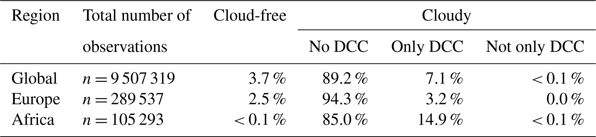
We considered a full year (2007) of MODIS and CloudSat-CALIPSO observations. The initial database consisted of 175 666 879 matchups. In order to maximize data consistency, all MODIS data were parallax-corrected following the method reported in Wang et al. (2011). We decided to narrow the sample by rejecting observations that were too warm to feature a DCC. Specifically, all observations with T_bIR−T_bWV < −10 K were rejected. This procedure was implemented by Yang et al. (2023), although the authors used a stricter threshold of −5 K. We used a more liberal threshold in order to increase the number of potentially non-DCC clouds in the vicinity of a DCC. This left 9 507 319 matchups that were evaluated. Table 1 provides more details on the composition of the sample.

Table 1 Cloud-free (no DCC) and cloudy (DCCs and other cloud types present) percentages in the lidar–radar profile data sample investigated in this study. Europe is defined as 35–60° N, 15° W–45° E, and Africa is defined as 5–15° N, 20° W–35° E (see Sect. 3 for details on subregions).

2.2 DCC detection methods

We assess the accuracy of the following three IR-based methods.

• The infrared-window (IRW) method. In principle, this method is very simple. The only requirement is to set a T_b value that can discriminate between DCCs (assumed to be colder) and a warmer background (either a cloudy or a cloud-free atmosphere). There is no universal T_bIR threshold for DCC detection, and different values have been used. Examples include 210 K (Aumann and Ruzmaikin, 2013), 225 K (Aumann et al., 2018), 230 K (Hendon and Woodberry, 1993; Tissier and Legras, 2016), 235 K (Wall et al., 2018), and up to 245 K (Kubar et al., 2007). This ambiguity in threshold selection is reflected in studies by Mapes and Houze (1993) and Hong et al. (2006), who decided to adopt two values: T_bIR < 235 K for the detection of high clouds in general and T_bIR < 208/210 K exclusively for DCCs.

• The brightness temperature difference (BTD) method. In earlier work, Ackerman (1996) observed that in some regions, T_b at 6.7 µm could be greater than that at 11 µm. In the tropics and midlatitudes, the T_bWV−T_bIR difference was explained by the presence of thick clouds, notably DCCs. In general, a difference greater than 0 K coincides with clouds of T_bIR < 210/215 K, and the difference is highest when clouds reach the tropopause (Kolat et al., 2013). Although Ackerman (1996) suggested that T_bWV−T_bIR could be used to detect thermal inversion in the polar troposphere, the method has been widely used to map DCCs, including the detection of overshooting tops (Bedka et al., 2010; Martin et al., 2008).

• The TROPO method. Convective clouds cool as their tops penetrate up through the troposphere, and eventually the cloud top temperature matches that of the tropopause. Hence, the difference between T_bIR and the tropopause temperature (T_tropo) has been suggested as a DCC detection method. Zou et al. (2021) used T_bIR at 8.1 µm and suggested that a feature could be considered a DCC when T_bIR−T_tropo ≤ 7 K. A similar value (6 K) was adopted by da Silva Neto (2016), who used T_bIR−T_tropo at the same time as a more conventional T_bWV−T_bIR approach. Aumann and Ruzmaikin (2013) set a T_bIR−T_tropo threshold of 2 K but used a climatological T_tropo value instead of an actual (meteorological) value. The application of the TROPO method relies on T_tropo data being available. In this study, the parameter was obtained from the Reanalysis Tropopause Data Repository (Hoffmann and Spang, 2022). Specifically, we refer to the first tropopause as defined by the World Meteorological Organization and identified based on the ERA5 reanalysis.

The ISCCP scheme for DCC detection only was included for comparison. In the ISCCP approach, the cloud type classification is based on cloud optical thickness (COT), and cloud top pressure (CTP). Like the IRW, BTD, and TROPO methods, the ISCCP requires thresholds – for COT and CTP – which are also somewhat arbitrary (Rossow and Schiffer, 1999). Hahn et al. (2001) demonstrated that the ISCCP classes follow the traditional classification (i.e. the one implemented by the World Metrological Organization) but follow them less strictly. Under the ISCCP paradigm, DCC detection requires COT and CTP information. Both were obtained from the MODIS MYD06 standard product (Platnick et al., 2003), with geometry and coverage that are identical to the MYD21KM and MYD03 products. ISCCP results only refer to daytime conditions, while the IRW, BTD, and TROPO results are combined for day and night.

2.3 Measures of accuracy

The joint CloudSat-CALIPSO cloud classification was used as a reference. MODIS WV, IR T_b, COT, and CTP data were used in the IRW, BTD, TROPO, and ISCCP methods to detect DCCs. Agreement between the reference and validated methods was assessed based on a confusion matrix and related measures.

A confusion matrix is used to evaluate the performance of a binary classifier. It considers four possibilities: true-positive and true-negative detection, when a method and the reference agree on the presence or absence of DCCs, respectively; false-positive detection, when a method finds DCCs but the reference does not; and false-negative detection, when a method reports no DCCs but the reference does. The performance of a DCC detection algorithm can then be assessed with respect to its overall accuracy, the probability of DCC detection (PoD), the DCC false-discovery rate (FAR), and Cohen's Kappa coefficient (κ; Cohen, 1960):

$$\begin{array}{}\text{(1)}& {\displaystyle }\mathrm{Accuracy}={\displaystyle \frac{\mathrm{TP}+\mathrm{TN}}{\mathrm{TP}+\mathrm{TN}+\mathrm{FP}+\mathrm{FN}}},\text{(2)}& {\displaystyle }\mathrm{PoD}={\displaystyle \frac{\mathrm{TP}}{\mathrm{TP}+\mathrm{FN}}},\text{(3)}& {\displaystyle }\mathrm{FAR}={\displaystyle \frac{\mathrm{FP}}{\mathrm{FP}+\mathrm{TP}}},\text{(4)}& {\displaystyle }\mathit{\kappa }={\displaystyle \frac{\mathrm{2}\cdot \left(\mathrm{TP}\cdot \mathrm{TN}-\mathrm{FP}\cdot \mathrm{FN}\right)}{\left(\mathrm{TP}+\mathrm{FN}\right)\cdot \left(\mathrm{FN}+\mathrm{TN}\right)+\left(\mathrm{TP}+\mathrm{FP}\right)\cdot \left(\mathrm{FP}+\mathrm{TN}\right)}},\end{array}$$

where TP, TN, FP, and FN are the total number (counts) of true-positive, true-negative, false-positive, and false-negative detections, respectively.

Values for a perfect classifier would be the following: accuracy and PoD equal to 100 %, FAR as low as 0 %, and κ approaching 1.0 (κ approaching 0.0 suggests that agreement between datasets was only achieved by chance regardless of the actual accuracy).

DCCs only made up 7 % of the CloudSat-CALIPSO observations investigated in this study, meaning that the sample was significantly unbalanced. It is reasonable to assume that the resulting accuracy measures are biased by the frequency of negative detections, which are far more likely than positive detections. To avoid this, we implemented bootstrap sampling (DiCiccio and Efron, 1996; Efron, 1979). First, the number of DCCs in our CloudSat-CALIPSO reference dataset was determined. Then the reference dataset was randomly sampled to identify exactly the same number of non-DCC observations. As a result, the count of DCC and non-DCC detections was equal. Next, instantaneous accuracy measures were derived from this subsample and recorded. This procedure was repeated 1000 times, resulting in 1000 accuracy estimations. In the final step, all estimations were averaged, returning a single value (a bootstrap estimate), which is reported in this paper. During each iteration, the DCC sample was the same and only the non-DCC subsample changed.

3 Results

Rather than assuming a specific threshold for a DCC detection method, we tested a wide range of possible values (Fig. 1). First, the full statistics were derived for each instantaneous threshold, then we selected the threshold with the highest overall accuracy (or the highest κ value, as both measures peaked at the same location). This value was then considered the optimal threshold, indicating that it guaranteed the best-possible accuracy for a method.

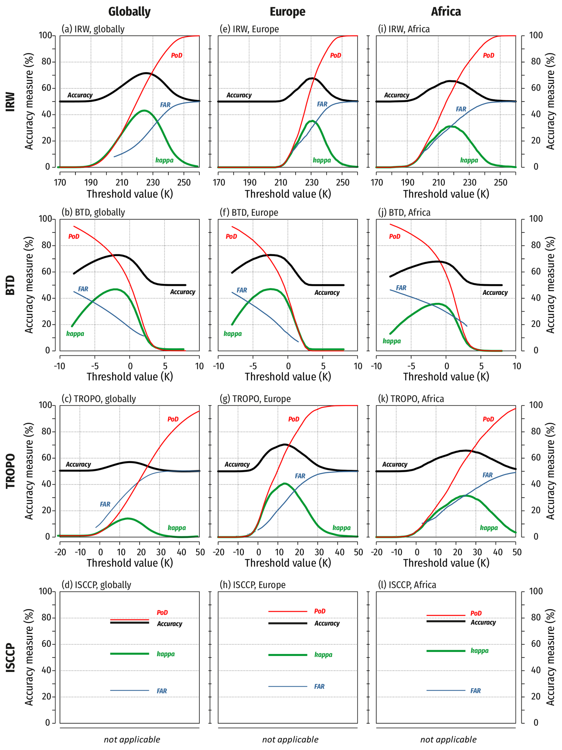
Figure 1 Accuracy of DCC detections using the infrared-window (IRW) method, the WV-IR brightness temperature difference (BTD) method, the IR − tropopause temperature difference (TROPO) method, and the ISCCP method. Accuracy measures are shown as a function of the selected threshold (horizontal axis), except for ISCCP, which uses a single set of parameters globally. Kappa (κ) values were multiplied by 100 to match the 0 %–100 % range.

All results were obtained for land and ocean lying between 60° N and 60° S (the global domain) and for two smaller regions of interest: Europe (a midlatitude moist convection environment; 35–60° N, 15° W–45° E) and equatorial Africa (an intertropical convergence zone with very intense moist convection; 5–15° N, 20° W–35° E).

3.1 Highest achievable accuracy

The validation of the IR-only DCC detection methods obtained with the CloudSat-CALIPSO lidar–radar dataset showed that the highest achievable accuracy was moderate (Fig. 1). Depending on the method and on a global scale, it varied between 56.6 % (TROPO with a 15 K threshold) and 72.9 % (BTD with a −2 K threshold). Regionally, accuracies were between 67.7 % (IRW with a 231 K threshold) and 72.9 % (BTD with a −2.5 K threshold) for Europe and from 65.6 % (IRW with a 217 K threshold) to 67.9 % (BTD with a −1 K threshold) for Africa.

Our results showed that the IRW and BTD methods performed almost equally well when global data were examined. Differences in overall accuracy, detection probability, and the false-alarm rate did not exceed ∼ 5 % at the global scale. However, changing the spatial domain to Europe doubled discrepancies; the IRW method was less accurate, while the BTD method performed just as efficiently as on the global scale. On the other hand, the comparison for tropical Africa found that both the IRW and BTD methods were less accurate.

Narrowing the spatial scale had the most significant impact on the performance of the TROPO approach. Using a single global threshold for the temperature difference between 10.8 µm and the tropopause proved impractical – the method detected DCCs with an overall accuracy of 56.6 % and a κ coefficient of 0.13. At the regional scale, performance noticeably improved: DCC detection probabilities doubled from 30 % to 60 %, resulting in a boost in overall accuracy of 14 % in Europe and 9 % in tropical Africa.

When the IRW, BTD, and TROPO methods were compared with the ISCCP daytime-only approach, the latter was found to be more reliable in all respects. Not only did it outperform the other methods with respect to overall accuracy (76 %–77 % regardless of the spatial domain), but the DCC detection probability was also higher (80 %–85 %), and, in general, the false-alarm rate was lowest among all of the methods investigated (25 %–28 %).

3.2 Variability in thresholds

Inconsistency between global and regional results motivated us to test whether the optimal threshold for a method depended on the latitude. We therefore derived accuracy measures for zones of 5° in latitude, starting at the Equator. Calculation of the accuracy for 5° zones essentially repeated the methods used for the global domain, except for the input data preselection: they were only limited to the 5° zone under consideration. With only 1 full year of observations, it was impossible to obtain reliable results for latitudes above 40–50° N/S (i.e. where DCCs are relatively infrequent).

Our experiment revealed a clear relation between latitude and the optimal threshold. For the IRW method, DCC detection across all latitudes was most accurate when the threshold was changed from ∼ 218 K in the tropics to ∼ 230 K in the midlatitudes. The corresponding adjustment for the BTD method was only 2 K (from −1 K in the tropics to −3 K in the midlatitudes). Similarly, for the TROPO method, the optimal threshold changed between the low latitudes and midlatitudes. However, in this case, in the tropics (20° S–20° N) it was constant (25 K), but it dynamically decreased (to 10–15 K) at 40° N/S.

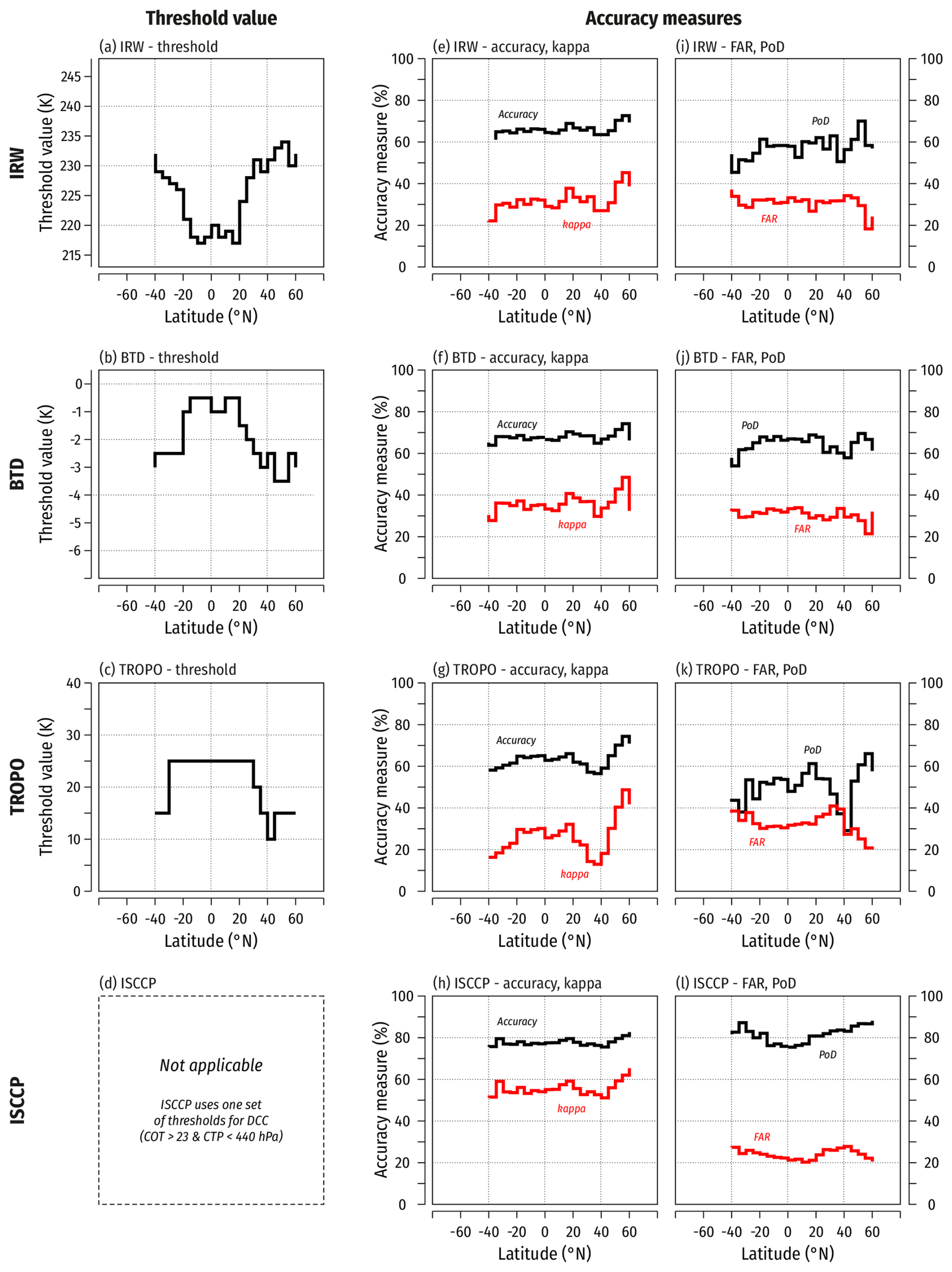
Figure 2 The optimal threshold for each method as a function of latitude (a–c), together with corresponding latitude-resolved measures of accuracy. Kappa (κ) values were multiplied by 100 to match the 0 %–100 % range.

Despite these adjustments in the threshold for different latitudes, the resulting DCC detection accuracy differed between zones. Variability was greatest for the TROPO method, with ∼ 15 % amplitude for the overall accuracy index (Fig. 2g) and an even more evident difference for the κ coefficient (from 0.15 to 0.5; Fig. 2g). Additionally, the highest and lowest scores differed most over the Northern Hemisphere (30 and 50° N). While this pattern was common to all methods, it was much less apparent (by 50 %) for the IRW (Fig. 2e) and BTD (Fig. 2f) methods compared to TROPO.

Compared to IR-based approaches, the ISCCP DCC detection scheme performed almost equally well at all latitudes. The DCC detection probability remained high (80 %–90 %), and the false-alarm rate was relatively low (20 %–30 %), resulting in a constant overall accuracy of ∼ 78 %–80 % regardless of the latitude. Like IR-based methods, the ISCCP scheme performed better in the northern midlatitudes, but the improvement was small and was mostly seen in an increasing κ coefficient (the consequence of a slight increase in detection probability).

3.3 DCC misclassification

Accuracy below 100 % necessarily indicates a certain degree of DCC misdetection by a given method. This could be either false negatives, when CloudSat-CALIPSO indicated a DCC but a method reported no DCC, or false positives, when reference data recorded no DCC, but a method reported one. In our study, false positives accounted for 8 %–17 % of observations (mean 13 %), while false negatives constituted 8 %–15 % (mean 17 %) depending on the method and the spatial domain (global, Europe, or tropical Africa).

The lowest rate of false-negative detections (8 %–10 %) was found for the ISCCP method, but when only the IR method was considered, it was 15 % at best for the BTD method regardless of the subregion of the study. Globally and over Europe, DCCs were most frequently missed by the TROPO method (35 % and 19 % of cases, respectively), while in Africa they were missed by the IRW method (23 % of cases). The better performance of the BTD method was at the price of a higher rate of false-positive detections: the methods classified non-DCCs as DCCs in 12 % (Europe, global) and 17 % (Africa) of cases.

Since CloudSat-CALIPSO data label clouds at each level in the atmospheric profile, we were able to identify typical scenarios where a non-DCC observation was mislabelled as a DCC. We identified two underlying patterns. First, three types of clouds were most frequently (> 90 % of cases) misclassified as DCCs: high clouds, As, and Ns. Second, which of these three types dominated depended on whether we investigated a single- or a multilayer cloud scenario (Table 2).

Table 2 Percentage of cloud types classified by the four methods as DCC but not reported as DCC in the CloudSat-CALIPSO observations. When more than one cloud layer occurred in a lidar–radar profile, the cloud type refers to the highest layer (i.e. the first to be observed when looking from a satellite).

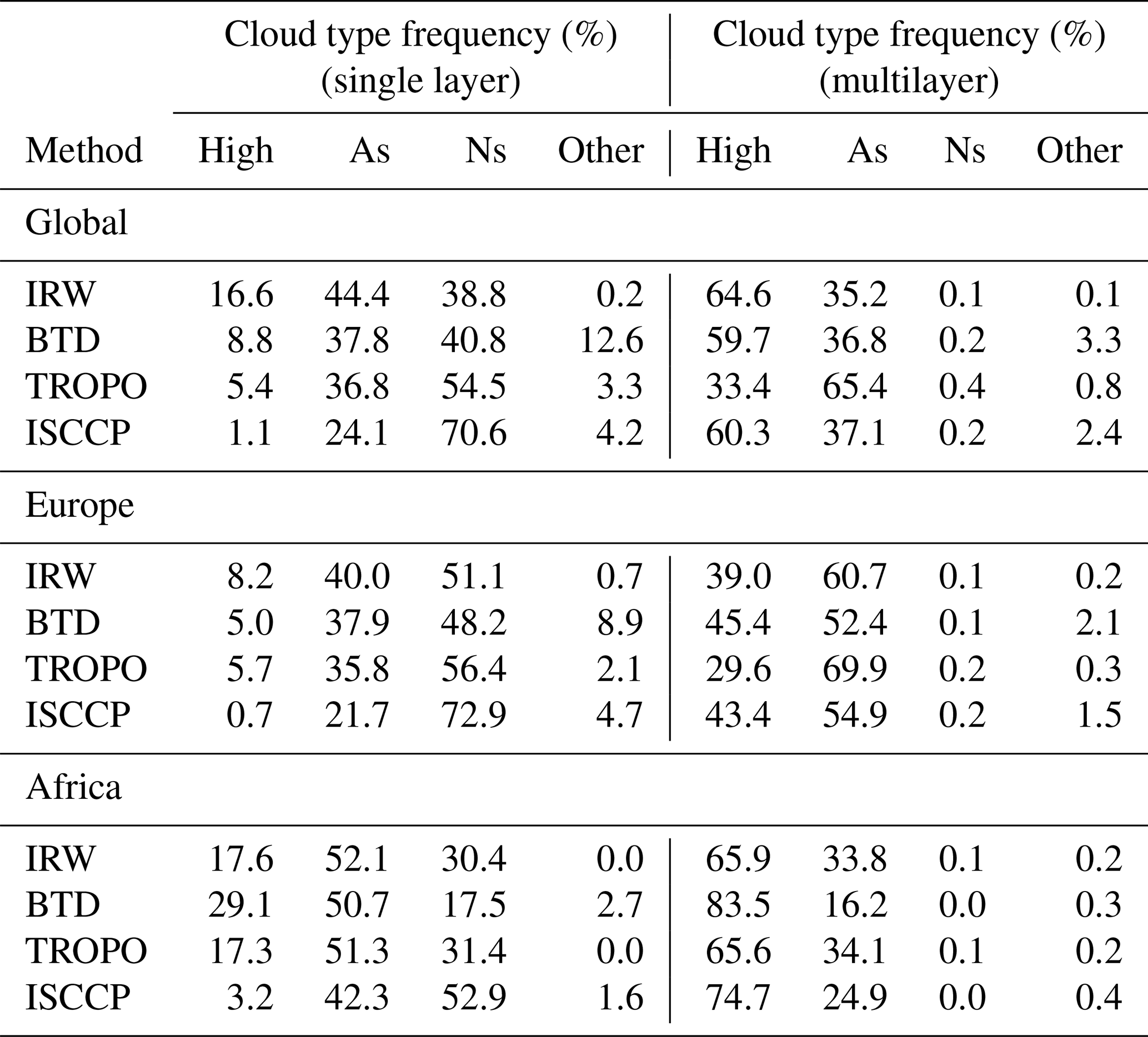
IR-based methods classified As and Ns as DCCs most frequently when clouds occurred as a single layer. This error accounted for over 35 % of misclassifications for each cloud type – both globally and for Europe. However, in tropical Africa, high clouds were more often mislabelled as DCC, although never as frequently as As or Ns were (with the exception of in the BTD method).

The situation changed significantly in a multilayer cloud environment. In this scenario, we only focused on the top-most (highest) cloud layer – the first to be detected when sensing from orbit. Our results showed that under such circumstances, IR methods falsely reported DCCs when the atmospheric profile was topped with As or high (cirrus-like) clouds. The co-occurrence of high clouds with other cloud types was the most challenging scenario, as this constituted up to 66 % (TRW, TROPO) or 84 % (BTD) of false-positive detections. In the multilayer environment, Ns were not a problem; they accounted for 0.4 % of erroneous cases regardless of the method or the region.

It is important to note that the As and Ns that were misclassified were the coolest clouds of their kind. The initial database of CloudSat/CALIPSO-MODIS matchups was screened for observations that satisfied the condition T_bWV−T_bIR > −10 K. Hence, all warm clouds, including a large share of As/Ns, were automatically excluded from further analysis. In the initial database of 175 million lidar–radar profiles, 50 % of observations had T_bIR in the range of 250–282 K. After filtering (9.5 million profiles), the range shifted towards a noticeably colder regime spanning 225–240 K.

3.4 Sensitivity to the selection of a threshold

Once we had calculated the optimal threshold for each DCC detection method, we then calculated the mean seasonal DCC frequency for June–July–August 2005. The thresholds identified in the present study were applied to an independent dataset, namely the geostationary Meteosat Second Generation data, which is collected hourly (every full hour). We used the High Rate Level 1.5 Image Data product based on Spinning Enhanced Visible and InfraRed Imager (SEVIRI) observations in two heritage bands: 6.25 and 10.8 µm (Holmlund et al., 2021). Data were accessed from the EUMETSAT archive (https://data.eumetsat.int/, last access: 23 June 2025). The geostationary perspective enables observations of approximately half of Earth's surface – a hemisphere that is centred at a sub-satellite point (0° E, 0° N in the case of Meteosat). Hereinafter we refer to that coverage as the Meteosat full disc. For practical reasons, the analysis only considers a fraction of the full disc data, i.e. the location within SEVIRI's zenith angle below 70° (see Fig. 3). The definitions of Europe and tropical Africa remained unchanged.

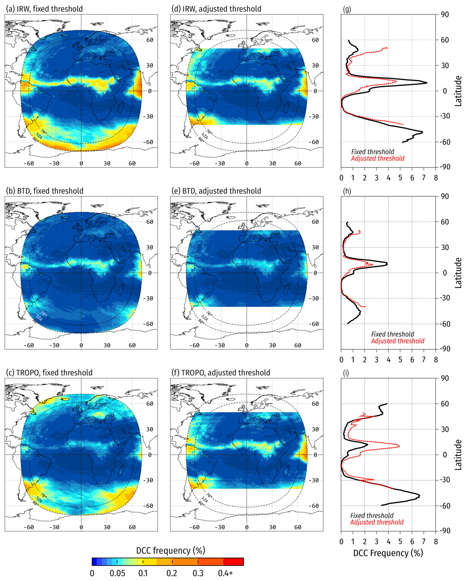
Figure 3 Mean seasonal (June–July–August 2005) DCC frequency based on hourly Meteosat/SEVIRI data and the methods evaluated in this study. Statistics were calculated using a fixed global threshold (a–c) or latitude-adjusted thresholds (d–f); panels (d)–(i) summarize zonally averaged DCC frequencies. The frequencies are given in the range of 〈0,1〉, where 0.0 indicates a DCC-free sky and 1.0 indicates DCCs occurring consistently across the sky.

A sensitivity study provided two sets of statistics. In the first set, we adopted fixed thresholds of 226.0 K for the IRW method, −2.0 K for the BTD method, and 15.0 K for the TROPO method (Fig. 3a–c). For the second set of statistics we used thresholds developed for each 5° latitude zone (Fig. 3d–f). As the results of testing different latitudes (Sect. 3.2) only covered 1 year of observations, the transition in threshold values between zones was not smooth (Fig. 2a–c), impacting the spatial distribution of DCCs (Fig. 3d–f). It is likely that artefacts could be eliminated with more data and that the change in threshold could be continuous rather than incremental – however, both of these refinements were beyond the scope of this study.

Table 3 Mean seasonal (June–July–August 2005) DCC frequency estimated using a fixed global threshold or a latitude-adjusted threshold. The frequencies are given in the range of 〈0,1〉, where 0.0 indicates a DCC-free sky and 1.0 indicates DCCs occurring consistently across the sky.

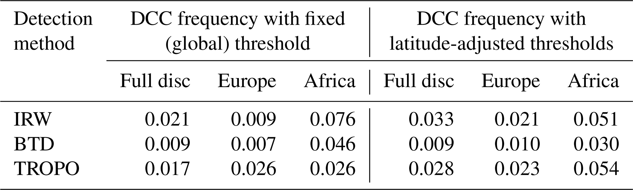
DCC detection frequencies for the two approaches differed substantially from each other (Table 3), demonstrating that the threshold selection significantly impacted the resulting DCC climatology. In the most extreme cases (the IRW method for Europe and the TROPO method for Africa), latitude-adjusted thresholds doubled the frequency of DCC occurrence compared to the fixed-threshold approach. For the remaining situations, the relative differences were lower (±30 % of DCC frequency) and in two cases did not exceed ∼ 10 % (the BTD method adopted globally and the TROPO method applied to Europe).

Figure 3g–i show that the tropics were most sensitive to threshold selection. Changing from a fixed global threshold to a regionally adjusted threshold reduced DCC frequency along the Intertropical Convergence Zone (ITCZ) when using the IRW or BTD methods (by one-third in relative terms) but increased DCC frequency for the TROPO method (rates at least doubled). The ITCZ was a dominant feature on DCC frequency maps – but only when the BTD method was used (Fig. 3b, e). ITCZ-comparable (or even higher) DCC frequencies were noted over the Southern Ocean (IRW, TROPO; Fig. 3g, i) and over mountainous regions of Europe (the Alps, the Carpathians). The latter finding was particularly apparent when using the TROPO method with a fixed global threshold (Fig. 3c) and for the IRW method with a regionally adjusted threshold (Fig. 3d). On the other hand, higher frequencies of DCCs over the Southern Ocean may not be due to the presence of actual DCCs but rather an effect of the misclassification of cold clouds as DCCs.

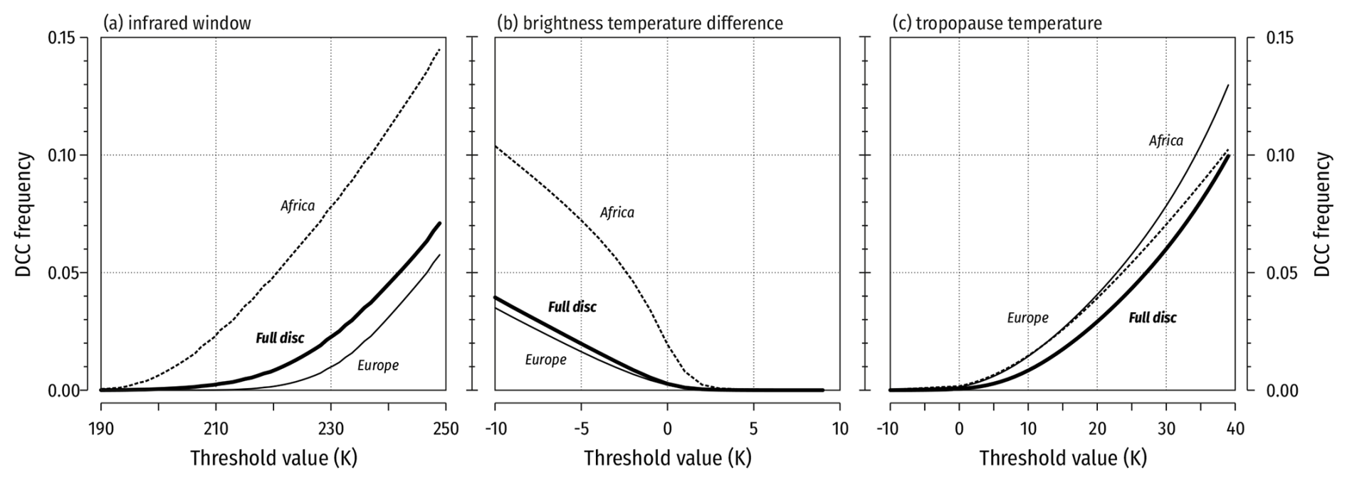
Figure 4 Mean seasonal (June–July–August 2005) DCC frequency as a function of the threshold applied to the DCC detection methods evaluated in this study. The frequencies are given in the range of 〈0,1〉, where 0.0 indicates a DCC-free sky and 1.0 indicates DCCs occurring consistently across the sky.

To explore the sensitivity of DCC climatology to threshold selection in more detail, we calculated DCC frequency as a function of the threshold value (Fig. 4). The slope of the DCC frequency curve is the most important information to consider when testing sensitivity: a steep slope indicates a relatively large change in DCC frequency for a small change in the threshold value.

We observed that for the IRW (Fig. 4a) and BTD (Fig. 4b) methods, the tropics (Africa) stood out as most sensitive to the choice of threshold. A shift of ±1–2 K in the threshold resulted in a change in DCC frequency that was 2 times larger than the corresponding change over Europe or at the global (full-disc) scale. However, the same was not true for the TROPO method. This was due to an increase in sensitivity observed for Europe and the full disc (Fig. 4c): while the slope of the sensitivity curve for both of these regions remained low when using the IRW and BTD methods, it became as steep as the one noted for the tropics when using the TROPO method. Consequently, the TROPO method was identified as the most sensitive to the threshold value – regardless of the region it was applied to. On the other hand, the BTD approach was least sensitive to a change (the most desirable result), except for in the tropics.

DCCs are very infrequent phenomena. Their frequency of occurrence is < 0.1, on a scale where 0.0 means no DCC at all and 1.0 indicates their permanent presence. A small change in that frequency (in terms of percentage points) translates into a high relative change. Here, we define relative change as the difference between the new value and the reference value divided by the reference value. For the data presented in Table 4, the reference was the full-disc DCC frequency with a fixed threshold, while the new DCC value was calculated using a threshold increased (or decreased) by 1 K.

Table 4 Mean seasonal (June–July–August 2005) DCC frequency calculated using a fixed global threshold (the reference DCC frequency) and with thresholds increased and decreased by 1 K. Values given in parentheses denote relative change, in other words, the difference between the reference DCC frequency and the frequency after the threshold change, normalized with reference to the DCC frequency. The frequencies are given in the range of 〈0,1〉, where 0.0 indicates a DCC-free sky and 1.0 indicates DCCs occurring consistently across the sky.

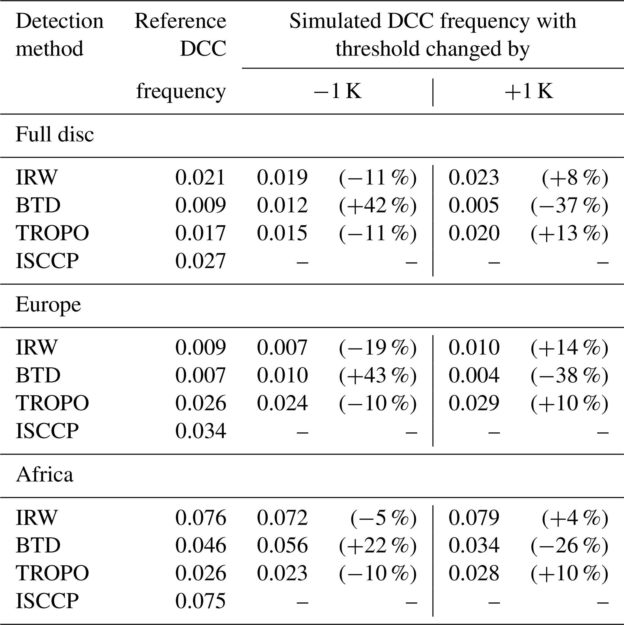
Table 4 reveals that a change in the threshold of as little as 1 K can substantially affect the final climatological estimate of DCC frequency. In the case of the BTD method, a ±1 K shift led to a ∼ 40 % relative change in DCC frequency, meaning that the frequency increased or decreased by nearly half of its absolute value (∼ 0.01 for Europe and globally). An equally significant relative change was found for the full disc and Europe, while Africa was close behind (∼ 20 % relative change, 0.01 absolute value). Comparisons of the other methods revealed relative differences in DCC frequency of 4 %–19 %; typically values were close to ∼ 10 %.

4 Discussion

4.1 Misclassification of DCC

In this study, we evaluated three IR methods that are widely used to detect DCCs. We found that even when the optimal configuration is adopted, either globally or regionally, the final accuracy of the algorithm is only moderate (up to 73 %). One factor that may have impacted our results is the reliability of reference data, namely the accuracy of the CloudSat-CALIPSO cloud classification product (2B-CLDCLASS-LIDAR).

Table 5 DCC detection accuracy in the tropics (±25° N). DCCs are defined as the merged CloudSat-CALIPSO DCCs and the nimbostratus classes (as in Yang et al., 2023) and as DCC alone (as in this study). The IRW method uses a threshold of 215 K, while the BTD method adopts a threshold of 0 K.

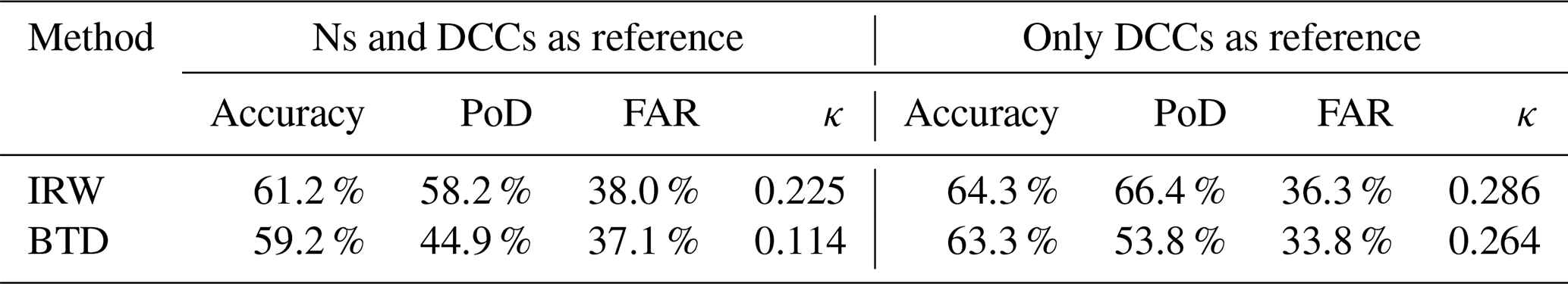
Assessments of the CloudSat-CALIPSO cloud typing algorithm revealed partial disagreement in DCC frequencies between lidar–radar and other datasets, namely satellite-based ISCCP climatology and surface-based visual (manual) classification (Wang and Sassen, 2001; Sassen and Wang, 2008; Sarkar et al., 2022). Specifically, As and Ns clouds tended to be reported more frequently in CloudSat data than in the datasets mentioned. Such overrepresentation could explain why these two cloud types were also the ones most frequently considered to be DCCs by the IR method but considered non-DCC by the lidar–radar reference. Possibly some As and Ns were actually DCCs and hence should be considered DCCs in the CloudSat-CALIPSO reference used in this study. Such a procedure was implemented by Yang et al. (2023), who validated IR-based DCC detection methods in the tropics (25° S–25° N). The authors decided to merge Ns and DCCs into one category and use it as a reference for DCCs. To test how such a strategy impacts detection accuracy, we repeated the Yang et al. (2023) study with two variants: with and without Ns in the reference. The results showed (Table 5) that the final accuracies were 4 %–5 % higher when Ns clouds were omitted but did not differ significantly. We conclude that not combining Ns with DCCs in our study had little impact on the final results.

In the multilayer scenario, cloud misclassification was frequently the result of a method classifying high clouds (cirrus) as DCCs. This can be explained by the simple fact that IR-based methods rely on cloud top temperature. Cirrus clouds tend to be as cold as DCCs, and they can only be distinguished by examining their vertical extent or optical thickness. These parameters, however, are unavailable when IR and WV channels are considered. On the other hand, high clouds were also mislabelled as DCCs in many ISCCP observations. ISCCP data include COT; therefore it is reasonable to expect fewer misclassifications. Unfortunately, ISCCP COT data are column-integrated, and cirrus optical thickness is included in the optical thickness of underlying cloud layers (including Ns and As).

Table 6 Percentage of observations (%; n = 9 507 319) when an error of either omission (false-negative DCC) or commission (false-positive DCC) was detected. Results are given for three cloud co-occurrence scenarios: no clouds (0 layers; 4 % of cases), clouds only in one layer (32 % of cases), and multilayer clouds (2+ layers; 63 % of cases). The number of layers is according to CloudSat-CALIPSO observations.

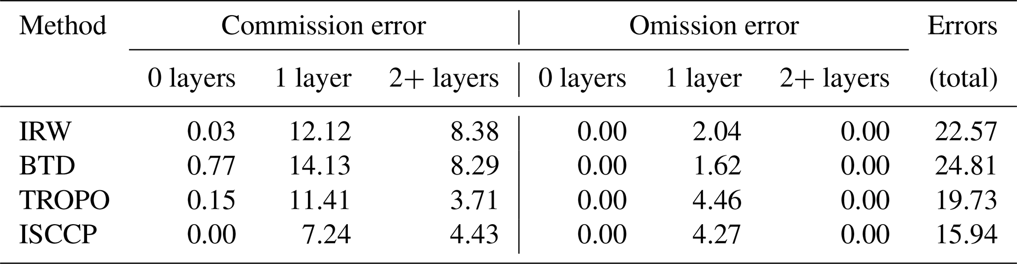
Misclassification errors were dominated by false-positive detections (errors of commission). Regardless of the IR-based method, this situation was found for 12 %–14 % of all observations under the single-layer scenario and for 4 %–8 % of observations under the multilayer scenario (Table 6). On the other hand, false-negative detections (errors of omission) only accounted for 2 %–5 % of observations and only occurred under the single-layer scenario. This means that the IR-based DCC detection algorithms investigated in this study are unlikely to miss a DCC. It is much more likely that they will identify a cloud as a DCC when it is not one. Consequently, they may lead to an overestimation of DCC extent or frequency.

Based on our results, we conclude that the main reason for DCC misclassification with the IR-based methods investigated is the scarcity of multispectral information. Brightness temperature is only known for one or two IR bands, and this is insufficient to correctly distinguish between the cold tops of DCCs and all other clouds that have similar thermal characteristics (e.g. cirrus or some elevated Ns). Expanding the range of spectral information, even indirectly (via products like COT or cloud top pressure/height), may improve detection performance, as demonstrated by the ISCCP climatology.

It is also important to realize that the limitations inherent in all types of cloud data make it impossible to develop a reference dataset that is 100 % correct. Although CloudSat-CALIPSO is widely considered to be the most reliable current option, it is not free from its own misclassification issues. Importantly, all of the IR-based methods we assessed in this study were validated against exactly the same (common) reference. Therefore, if even the reference dataset has limitations and actual (absolute) DCC detection accuracies may differ from those reported, relative differences between methods were captured correctly, and we were able to indicate which of them performed more or less efficiently.

4.2 Impact of matching geometry

A second factor that may have influenced the results of our study is the spatial and temporal collocation of lidar, radar, and MODIS observations. Each instrument was installed on a different satellite, meaning that a vertical atmospheric column was not observed simultaneously by all three sensors. In 2007, CloudSat (the Cloud Profiling Radar instrument) preceded CALIPSO (the Cloud–Aerosol Lidar with Orthogonal Polarization instrument) by ∼ 15 s and followed Aqua (MODIS) by approximately 1 min.

The horizontal speed of a storm cloud is ∼ 30–100 km h⁻¹, and a cloud could have shifted by ∼ 0.5–1.5 km during the minute that separated the MODIS and CloudSat-CALIPSO passes. This distance is generally within CloudSat's footprint (1.4 × 1.1 km), meaning that misclassification would only occur if CloudSat's ground track was collocated with the cloud's edge and if the cloud moved outward relative to the ground track.

It should also be noted that a cloud is a three-dimensional structure that evolves vertically, especially when it is a DCC with a strong updraught. Updraught intensity varies from a few metres per second for fair weather cumuli (Kollias et al., 2001) to 10–30 m s⁻¹ for tropical cyclones (Stern and Bryan, 2018) and 30–50 m s⁻¹ for the most rapidly evolving DCCs (Apke et al., 2018; Musil et al., 1991). Therefore, cloud top height can increase by between 500 m (updraught ∼ 8 m s⁻¹) and 2 km (updraught ∼ 30 m s⁻¹) over 1 min, corresponding to a decrease in cloud top temperature of 3–12 K (assuming a rate of 6 K km⁻¹). This creates a situation where CloudSat-CALIPSO could have detected a DCC that was not yet detected as a DCC by MODIS: the imager observed a cloud a few kelvins before it became a DCC.

The aforementioned scenario would result in more false negatives, reducing the overall accuracy of IR-based methods compared to a scenario in which all sensors operated in collocated mode. The latter could be achieved if lidar, radar, and imager instruments were installed on the same platform, which is the case for the Earth Clouds, Aerosol, and Radiation Explorer (EarthCARE) satellite. The satellite was launched in 2024 and is in the commissioning phase at the time of writing.

EarthCARE hosts not only lidar and radar instruments but also a seven-channel multispectral imager that covers three IR bands: 8.8, 10.8, and 12.0 µm (Illingworth et al., 2015). The setup eliminates all uncertainties related to spatial and temporal mismatches in a DCC observation. Unfortunately, the imager does not operate in the WV absorption bands, ruling out the use of the two-channel DCC detection method. This situation is similar to CALIPSO's imager, the Imaging Infrared Radiometer (IIR), which operated in three bands (8.7, 10.5, 12.0 µm). However, none of these channels consider WV absorption, as the sensor was optimized for joint CALIOP–IIR retrievals of cirrus microphysical parameters.

Importantly, EarthCARE's radar – unlike CloudSat's – is a Doppler instrument. It provides data on the vertical velocity of hydrometeors (cloud particles, rain) with an accuracy better than 1.3 m s⁻¹ (Wehr et al., 2023). This may improve discrimination between cloud types and provide more accurate labelling of DCCs for not only validation but also training various machine learning models (Afzali Gorooh et al., 2020; Kaps et al., 2024). Nonetheless, the use of imagers that include WV absorption bands makes MODIS-CloudSat-CALIPSO joint observations unique and the most suitable for the evaluation of DCC detection methods.

4.3 Implications for cloud climatology

Given the limitations of the MODIS-CloudSat-CALIPSO cloud observing system and based on our results, we conclude that the T_bWV−T_bIR brightness difference (BTD) method is slightly more robust among the algorithms evaluated. Accuracy was highest, as was the κ coefficient, indicating the best agreement with the CloudSat-CALIPSO reference data. On the other hand, the BTD method resulted in the lowest DCC frequency among all of the algorithms considered, which, in turn, impacted the method's sensitivity to the threshold selection. Importantly, we found that the optimal global threshold was −2 K (−1 K in the tropics, −3 K in the midlatitudes). These values differ from a typical threshold of 0 K. Since higher thresholds lower the DCC frequency, the adoption of a 0 K threshold may underestimate DCC frequency compared to the CloudSat-CALIPSO dataset.

The BTD method requires data from the IR-window and water vapour (WV) absorption channels, and it can be easily applied to all generations of meteorological geostationary satellites. It supports the development of long-term (more than 40 years) DCC climatologies and composite DCC maps generated with data from various geostationary platforms such as the NCEP/CPC Level 3 Merged Infrared Brightness Temperatures product, the NASA SatCORPS Global Cloud Composite product, or the GEO-ring composites envisioned for the ISCCP-Next Generation project.

The WV absorption band is typically not included on imagers that are hosted on polar-orbiting platforms. Examples include the Advanced Very High Resolution Radiometer (NOAA-6/19, MetOp), the Visible/Infrared Imager Radiometer Suite (SNPP, NOAA-20/21, JPSS-3/4), the Multichannel Visible Infrared Scanning Radiometer (Feng-Yun-1 series), the Visible and Infrared Radiometer (Feng-Yun-3A/C), and the VIS/IR Imaging Radiometer (Meteor-M series). Although these instruments have been used since the late 1970s or early 1980s, none feature a spectral band in the 6.5 µm WV absorption region.

Detecting DCCs without the WV band requires using the single-channel IRW method or IR-window data with auxiliary information on the tropopause temperature (the TROPO method). In this case and when locally adjusted thresholds are used, the IRW and TROPO methods produce comparable results in terms of both overall agreement with CloudSat-CALIPSO and the spatial distribution of DCCs. We found that the TROPO method performed slightly better than the IRW approach but only for Europe and only by 3 %–4 %. This finding indicates that the inclusion of tropopause data does not necessarily lead to a significant improvement in DCC detection, at least when the analysis explores the difference between the tropopause temperature and cloud T_b.

Importantly, both the TROPO and IRW methods recorded unexpectedly high DCC frequency, mostly over the Southern Hemisphere (in winter). According to these methods, DCCs in these regions were as frequent as in the ITCZ, which is not confirmed by other datasets (e.g. Norris, 1998; Sarkar et al., 2022). We conclude that the TROPO and IRW approaches performed poorly at higher latitudes, overestimating the frequency of DCCs. This may have been due to a misclassification of cold-top Ns or As as DCCs, as these cloud types occur most frequently at higher latitudes (Chen et al., 2000). As a consequence, the IRW and TROPO methods may be of limited use during colder seasons at higher latitudes – however, this is the region that is sampled best by polar-orbiting spacecraft, and it is where climate change may impact DCC frequency the most.

Our Meteosat-based sensitivity study demonstrated that the selection of an appropriate threshold is crucial for deriving accurate DCC frequencies. This finding is important in order to be able to construct DCC climatologies from radiance time series originating from various sensors (different families of sensors or different generations within a single family). A 1 K difference in T_b may be a consequence of a difference in the spectral response function of different sensors, or it could be the consequence of the sensor's calibration (Gunshor et al., 2004). The same DCC observed simultaneously by two instruments may appear in the final dataset as an object with different T_b. Hence, using a single threshold for both datasets will produce incoherent DCC climatologies.

If we take the CloudSat-CALIPSO classification as a reference, our study reveals the limits of the most common IR-based DCC detection methods. Specifically, we identified thresholds that result in the highest achievable accuracy. However, better results can possibly be achieved with other methods. We also evaluated DCC statistics resulting from the ISCCP cloud typology. DCC detections based on COT and CTP were shown to be more reliable than any of the IR-based methods. This finding demonstrates that daytime DCC detection benefits from the availability of shortwave radiances.

More complex algorithms, such as machine learning, can be used to process IR-only data. For instance, Yang et al. (2023) trained their algorithm on T_b but also used a number of derivative measures that addressed local variation (minima, maxima, gradients). They achieved 72 % accuracy in DCC detection. Even higher accuracy (98 %) was reported by Chen et al. (2023), who considered texture information along with a sequence of images in three IR bands (6.25, 10.7, and 12.0 µm).

Since DCC detection requires both daytime and nighttime data, IR observations from cloud imagers will remain a primary source of information. This is especially true for long-term climate studies, as the WV absorption channel and the IR-window channel are the only two heritage bands that have been available on geostationary satellites since the early 1980s. Machine learning techniques that are trained on more sophisticated datasets (e.g. EarthCARE) offer the potential for more reliable and homogenous DCC climatologies that go beyond the limits of classical IR-based algorithms.

5 Summary and conclusions

Our study explored the consistency of DCC climatologies derived from three widely used IR-based DCC detection algorithms, namely: (1) the IR-window method (11 µm spectral channel), (2) the brightness temperature difference (BTD) between 6.7 and 11 µm, and (3) the temperature difference between the tropopause and the 11 µm channel (TROPO). These algorithms were applied to MODIS/Aqua radiances, and compared with the unique, state-of-the-art CloudSat-CALIPSO lidar–radar cloud classification dataset. We assumed CloudSat-CALIPSO as a reference (ground truth). However, it must be acknowledged that in cloud research, there is no universally reliable dataset, and in a strict sense, our study is a comparison with lidar–radar, which we consider the most reliable of the currently available data.

In total, 9 507 319 observations for 2007 were analysed, marking the first global-scale evaluation of these DCC detection methods. The two key conclusions from our study are as follows.

• IR-based methods demonstrate moderate accuracy in DCC detection (< 75 %; κ < 0.45) but only when regionally or zonally adjusted thresholds are used. Fixed globally applied thresholds should be avoided. Detection ambiguity arises from the misclassification of DCCs as Ns and As (in single-layer cloud scenarios) or as cirrus and As (in multilayer cloud scenarios). We conclude that these disagreements are partially due to the method's simplicity but also identified uncertainties in the CloudSat-CALIPSO cloud classification and imperfections in the observation system (notably, the temporal misalignment between lidar, radar, and imager observations).

• The high sensitivity of IR-based methods to threshold selection undermines the homogeneity of the resulting DCC climatologies. Our analysis demonstrates that shifting the threshold by as little as ±1 K leads to a change in mean seasonal DCC estimates of 0.002–0.010, which translates into a relative change of 4 %–40 %. This finding is of particular importance when combining IR data from different sensors, whether to construct global mosaics or to produce time series of DCCs from various generations of an instrument.

Assuming CloudSat-CALIPSO data to be ground truth, we conclude that if the WV absorption and IR-window channels are available, the BTD method should be prioritized over the IRW and TROPO methods (e.g. for geostationary satellites). If these channels are not available (as with most polar-orbiting platforms), the TROPO method may provide comparable results but at the cost of including auxiliary data on tropopause temperature. The IRW method should be considered a last resort for the detection of DCCs.

As technology progresses, the launch of new cloud imagers with more spectral channels (e.g. Flexible Combined Imager, GeoXO Imager, METimage) will enhance the accuracy of DCC detection. This improvement will be especially notable when new data sources are paired with new data processing technologies, such as machine learning. Nevertheless, the WV absorption channel and the IR-window channel remain the most important spectral bands for long-term DCC climate studies, along with the IR-based methods that utilize them.