Assessment and application of melting-layer simulations for spaceborne radars within the RTTOV-SCATT v13.1 model

Because of their high sensitivity to hydrometeors and high vertical resolutions, spaceborne radar observations are emerging as an undeniable asset for numerical weather prediction (NWP) applications. The EUMETSAT (European Organisation for the Exploitation of Meteorological Satellites) NWP SAF (Satellite Application Facility for Numerical Weather Prediction) released an active sensor module within version 13 of the RTTOV (Radiative Transfer for TIROS Operational Vertical Sounder) software with the goal of simulating both active and passive microwave instruments within a single framework using the same radiative transfer assumptions. This study provides an in-depth description of this radar simulator. In addition, this study proposes a revised version of the existing melting-layer parameterization scheme of Bauer (2001) within the RTTOV-SCATT v13.1 model to provide a better fit to observations below the freezing level. Simulations are performed with the revised and default schemes for the Dual-frequency Precipitation Radar (DPR) instrument on board the Global Precipitation Measurement (GPM) mission using the ARPEGE (Action de Recherche Petite Echelle Grande Echelle) global NWP model, operational at Météo-France for two different 1-month periods (June 2020 and January 2021). Results for a case study over the Atlantic Ocean show that the revised melting scheme produces more realistic simulations much closer to observations compared to the default scheme both at Ku (13.5 GHz) and Ka (35.5 GHz) frequencies. A statistical assessment covering several cases shows significant improvement of the first-guess departure statistics. As a step further, this study showcases the use of melting-layer simulations for the classification of precipitation (stratiform, convective, and transition) using the dual-frequency ratio (DFR) algorithm. The classification results reveal a significant overestimation of the rain reflectivities in both hemispheres, which could indicate either an overproduction of convective precipitation in ARPEGE or a misrepresentation of the convective precipitation fraction within the forward operator.

1 Introduction

Spaceborne radars at several frequencies (Ku: 13.5 GHz; Ka: 35.5 GHz; W: 94 GHz) offer the unique capability to observe clouds and precipitation in three dimensions and at the global scale (Battaglia et al., 2020). Observed radar reflectivity (Z) profiles have been widely used by both the climate and the numerical weather prediction (NWP) communities, mainly for validating global NWP model outputs (Bodas-Salcedo et al., 2008, 2011) but also for investigating the assimilation of these data (Fielding and Janisková, 2020; Ikuta et al., 2021a; Kotsuki et al., 2023). In particular, the CloudSat cloud-profiling radar (CPR) (Stephens et al., 2002) was used to validate global model forecast quality (e.g. UK Met Office Unified Model (MetUM) by Bodas-Salcedo et al., 2008; Global Climate Model (GCM) by Marchand et al., 2009; and European Centre for Medium-Range Weather Forecasts (ECMWF) Integrated Forecasting System (IFS) by Di Michele et al., 2012). Similarly, the Precipitation Radar (PR) on board the Tropical Rainfall Measuring Mission (TRMM) was used to evaluate precipitating cloud types and microphysics in a cloud-resolving model (CRM) in Matsui et al. (2009) and Li et al. (2008). Finally, the Dual-frequency Precipitation Radar (DPR) on board the Global Precipitation Measurement (GPM) mission (Hou et al., 2014) was used as a reference by Mai et al. (2023) to evaluate cloud microphysical properties in the Weather Research and Forecasting (WRF) model. A review of different operational applications of spaceborne precipitation radars is available in the International Precipitation Working Group (IPWG) report (Aonashi et al., 2021).

Using observations to evaluate a model directly requires the use of a radar simulator to transform model variables into radar reflectivities at model levels, the so-called model-to-satellite or forward approach, which is commonly used in data assimilation applications and climate model evaluation studies (Ringer et al., 2003). Many such simulators exist, e.g. Quickbeam (Haynes et al., 2007), Joint-Simulator (Hashino et al., 2013), ZmVar (Fielding and Janisková, 2020), Passive and Active Microwave TRAnsfer (PAMTRA) (Mech et al., 2020), Community Radiative Transfer Model (CRTM) (Moradi et al., 2023; Johnson et al., 2023), and Goddard Satellite Data Simulator Unit (G-SDSU) (Matsui et al., 2013, 2009). However, the Radiative Transfer for the TIROS¹ Observational Vertical Sounder (RTTOV) (Saunders et al., 2018) model, which is widely used in model-to-satellite simulations of passive radiances, particularly for NWP, has not provided a radar capability until very recently. This study presents the new radar simulator available in version 13 of RTTOV-SCATT which benefits from state-of-the-art developments for passive microwave simulations within clouds and precipitation (Geer et al., 2021).

Radar signals from precipitation radars are very difficult to model in the mixed-phase region (also called the melting layer), where hydrometeors are in transition between frozen and liquid states (Zhang et al., 2008). Inside the melting layer in nature, the snowflakes of maximum size are first transformed into wet flakes and then to raindrops of smaller sizes of equivalent mass and with lower number density as compared to the original flakes (Galligani et al., 2013). The large difference in permittivity between the two phases causes a sudden enhancement of reflectivity known as the “bright band” (hereafter, BB), which is most prominent in stratiform precipitation (Giangrande et al., 2008; Klaassen, 1988; Karrer et al., 2022). In addition to providing more accurate and realistic representations of the reflectivities at the freezing level, the accurate simulation of the bright band importantly allows more realistic profiles of attenuated reflectivity to be derived. Indeed, a bright band that is too strong attenuates the radar signal and impacts the attenuated reflectivity in the rainy layers below the melting layer, which could result in an underestimation of the rainfall.

In the past few years, simulation of the melting layer has been extensively investigated for ground-based radars (Klaassen, 1988; Szyrmer and Zawadzki, 1999; Boodoo et al., 2010; Iguchi et al., 2014; Augros et al., 2016; Das et al., 2023) but rather limited for spaceborne radars. For instance, Kollias and Albrecht (2005) simulated melting-layer reflectivities for CloudSat CPR and observed a small decrease in reflectivity (1–2 dB) just above the freezing level due to Mie backscattering effects, which they refer to as the “dark band”. Similar results are also found in the conclusions of Sassen et al. (2007, 2005) and Lhermitte (1988). Olson et al. (2001) used a steady-state melting-layer scheme to simulate TRMM PR reflectivities and noticed that melting precipitation can result in a 5 dB increase in the layer-mean reflectivity at the Ku band. Bauer (2001) presented a melting-layer scheme to compute scattering properties for both passive and active instruments, which is already available in RTTOV-SCATT. This scheme treated hydrometeors as homogeneous spheres. Geer and Baordo (2014) already introduced non-spherical shapes for frozen hydrometeors in RTTOV-SCATT for providing accurate simulations in the ice region but retain a Mie sphere representation of the melting layer. A few studies (Johnson et al., 2016; Petty and Huang, 2010; Botta et al., 2010) reported that non-spherical particle shapes better represent the early stage of melting where hydrometeor properties change very rapidly, but this is not considered in this study.

It is well known from past studies (Kollias and Albrecht, 2005; Romatschke, 2021) that while W band radars are excellent for observing clouds and light precipitation, they are not best suited for observing heavy precipitation due to greater attenuation and multiple scattering effects compared to lower-frequency radars. Furthermore, while a bright band can be seen at W band (e.g. Moradi et al., 2023), its peak is less intense than at lower radar frequencies. Therefore, this study focuses on Ku and Ka band radars to simulate bright-band signatures and to assess the benefits obtained by the use of a revisited parameterization of Bauer (2001).

In the observation world, the bright-band detection has several applications. One of them is precipitation type classification (Iguchi et al., 2010). Le and Chandrasekar (2012) proposed a dual-frequency ratio (DFR, e.g. difference between Ku and Ka band reflectivities) classification algorithm which is based on the vertical variation of the DFR within and below the melting layer. If the melting layer is detected, then the DFR algorithm is able to classify precipitation into three categories (i.e. stratiform, convective, and transition). In the areas where both frequencies are not available, the DFR algorithm is associated with another single-frequency algorithm for the precipitation type classification within the GPM DPR level 2 product (Huffman et al., 2018; Iguchi et al., 2010; Kobayashi et al., 2021; Awaka et al., 2016). The vertical variation of DFR is a base for the development of many other algorithms for DPR observations like the graupel and hail detection algorithm by Le and Chandrasekar (2021), as well as a surface snowfall detection algorithm by Le et al. (2017). Motivated by the success of the DFR algorithm on real observations, this study investigates whether the bright-band parameterization of RTTOV-SCATT has reached a sufficient degree of realism that the DFR algorithm can also be applied to NWP model profiles and, further, whether it can support the precipitation classification of NWP model profiles with a reasonable degree of accuracy.

Therefore, the present study has two objectives. The first objective is to present the upgrade of the melting-layer parameterization scheme in the RTTOV-SCATT model v13.1, with the upgrade now available in v13.2. This objective also validates the simulations for the DPR Ku–Ka instrument by comparing observations to simulations. The second objective is to investigate whether the bright-band simulations for Ku and Ka bands are realistic enough that they can be used for applications like precipitation type classification. The paper also functions as a first complete documentation of the RTTOV radar simulator in the peer-reviewed literature. The paper is organized as follows. Sect. 2 briefly describes the two datasets used in the study from the GPM/DPR instruments as well as the ARPEGE NWP model, Sect. 3 describes the RTTOV-SCATT radar forward operator and melting-layer parameterization schemes within the forward operator, Sect. 4 presents the impact of melting layer on reflectivity simulations on a case study and with co-located samples between the GPM/DPR and ARPEGE over a 2-month period. The DFR algorithm for precipitation classification is explained and applied to ARPEGE in Sect. 5, followed by the conclusions and perspectives in Sect. 6.

2 Data and models

2.1 GPM/DPR observations

The GPM mission was launched on 28 February 2014. It carries a dual-band (Ku and Ka) precipitation radar (DPR) that provides three-dimensional observations of clouds and precipitation for a wide range of latitudes (67° S–67° N) (Hou et al., 2014; Skofronick-Jackson et al., 2017). Both radars have a centre beamwidth of 0.71° and a footprint resolution of 5 km. The swath width of the Ku band radar is 245 km, and the one for the Ka band radar is 120 km. The minimum detectable signals are 18 and 12 dBZ for Ku and Ka bands, respectively (Hamada and Takayabu, 2016).

Version 6 of the 2A DPR product, which was created by combining Ku and Ka frequency radar echoes within the same scattering volume, is used in this study. The 2A DPR product has been used in many past studies for calibration, validation, and classification purposes (Kotsuki et al., 2014; Zhang and Fu, 2018; Sun et al., 2020). For example, Sun et al. (2020) used the 2A DPR product to classify stratiform and convective pixels to study vertical structures of the typical Meiyu precipitation event over China. The inner swath pixels (25) in match swath (MS) mode are used in this study, where both Ku and Ka bands are on the same grid and viewing exactly the same area as well as having the same vertical resolution of 250 m. Further details about the different modes of the DPR scan pattern are given in Hou et al. (2014). It has to be noted that MS pixels are oversampled to 125 m vertical resolution in the 2A DPR product. For this study, attenuated Ku and Ka reflectivity profiles, precipitation type, and quality flags are used.

Figure 1 shows an example of a single orbital file on 2 January 2021. For this particular orbit, the sensor followed the path starting at the black point and ending at the grey point. The black box depicted in the Atlantic Ocean is chosen for a case study as a first step before running a statistical study (more details are given in Sect. 4.2).

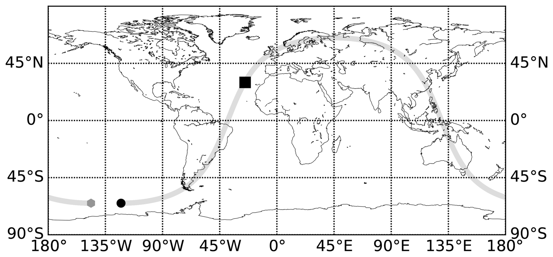
Figure 1 Ground track of one orbit of GPM for 2 January 2021. The black dot corresponds to the beginning of the orbit file and the grey dot to the end of it. The box represents the location of a single cloud over the Atlantic Ocean, which is used in Sect. 4.2 for the case study.

2.2 ARPEGE global NWP model

This study uses the ARPEGE NWP global model, which is operational at Météo-France since 1992 (Courtier, 1991). The latest operational configuration is used, which is characterized by a spectral resolution of T1798, used with a stretched and tilted grid giving a horizontal resolution of 5 km across Europe to 25 km at the antipodes (Aotearoa / New Zealand). Further details on the ARPEGE global NWP model are given in Bouyssel et al. (2022) and only briefly mentioned here. The model is characterized by 105 vertical levels, from ∼ 10 m above the ground to the model top at 0.1 hPa (∼ 70 km). The model uses a 6 h cycling 4D-Var (4D variational) incremental data assimilation scheme to generate analyses four times per day. The Ensemble of Data Assimilation of ARPEGE (AEARP; Desroziers et al., 1999) is used to compute the background error covariance matrix. ARPEGE makes use of six hydrometeor types to represent clouds and precipitation: four of them are prognostic variables (stratiform snow, stratiform rain, cloud liquid, water and cloud ice) with their evolution governed by the Lopez (2002) microphysical scheme and two of them (convective snow and convective rain) are diagnosed variables governed by the deep convective scheme of Tiedtke (1989). In this study, the ARPEGE model is set up for 2 different months: (a) 1–30 June 2020 (summer in Northern Hemisphere (NH) and winter in Southern Hemisphere (SH)) and (b) 1–31 January 2021 (winter in NH and summer in SH).

2.3 Collocation between ARPEGE model and observations

The choice is made in this study to compare observations and model forecasts in the short range only, at +6 h forecast range. Simulations and observations are vertically, horizontally, and temporally co-located. To avoid as much as possible time mismatches between observations and simulations, only the observations which are available within ±30 min surrounding the validity time of the +6 h forecasts are used for the comparisons against simulated observations. This temporal window is a good compromise to collect a sufficiently large number of cloudy and precipitating observations which are likely to still be valid at the time of comparisons.

Spatially, the nearest ARPEGE latitude–longitude grid point is allocated to each observed location. Di Michele et al. (2012) performed the averaging of radar profiles corresponding to the model grid box. However, averaging introduces additional uncertainty, especially when the clouds are non-homogeneous within a grid point. Performing such an averaging is also difficult for ARPEGE as the horizontal resolution varies with the latitude and longitude. The choice was made to not average DPR data at the model resolution in the study but to keep this information in mind when interpreting the results by hemisphere and geographical zones.

The reflectivity simulations with the ARPEGE model are generated at 105 height levels. However, DPR observations are available at 176 height levels (125 m each) at a finer vertical resolution. To remove the discrepancies between observed and model height levels, simulations are interpolated linearly in geometric height and in reflectivity (mm⁶ m⁻³). Note that when the simulated reflectivities above the sensitivity of the radar are not continuous in the vertical, these gaps are preserved in the interpolated profiles.

3 RTTOV-SCATT V13.1 forward operator

This study uses the RTTOV-SCATT (v13.1) radiative transfer model for the simulation of GPM/DPR reflectivities both at Ku and Ka bands (Geer et al., 2021). Note that RTTOV-SCATT also includes the tangent-linear (TL) and adjoint (AD) versions of the radar simulator. However, as this study is focused on the forward operator, they are not described here.

The inputs of the forward operator are profiles of temperature, pressure, specific humidity, hydrometeor contents, hydrometeor fractions, and sensor parameters (e.g. radar frequency, grid location, and viewing angle). For this study, a new feature of RTTOV allowing users to set an ensemble of hydrometeors has been used: the configuration used therefore takes into account the six hydrometeors classes (described in Sect. 2.2) of ARPEGE instead of only five hydrometeors in the default configuration. The forward operator uses the radar equation (Eq. 1) for the simulation of attenuated and unattenuated reflectivities at each radar range gate. Assuming the six categories of hydrometeors (i) and their particle size distributions (N_i), the reflectivity (mm⁶ m⁻³) is computed by integrating the backscattering cross-section σ_i(D) (m²) over the particle size distribution (PSD) within the size limits D_min to D_max. The total reflectivity is obtained after summing up the contributions from all six hydrometeors at each range gate which is at a distance R (m) from the radar. The signal value is very large in number; therefore, converting into a logarithmic scale (dBZ) is a standard way of using radar products in meteorology.

$$\begin{array}{}\text{(1)}& \begin{array}{rl}& Z\left(R\right)\left[\mathrm{dBZ}\right]=\mathrm{10}{\log }_{\mathrm{10}}\left({\mathrm{10}}^{\mathrm{18}}{\displaystyle \frac{{\mathit{\lambda }}^{\mathrm{4}}}{{\mathit{\pi }}^{\mathrm{5}}\mid K_{\mathrm{w}}{\mid }^{\mathrm{2}}}}A\left(R\right)\right.\\ & \left.\times \sum _{i=\mathrm{1}}^{\mathrm{6}}{f}_i\left(R\right)\underset{D_{\min }}{\overset{D_{\max }}{\int }}{\mathit{\sigma }}_i\left(D\right)N_i\mathit{\{}D,W_i(R\left)\mathit{\right\}}\mathrm{d}D\right)\end{array}\end{array}$$

Here, λ (m) is the radar wavelength (Ku ≈ 0.022 m, and Ka ≈ 0.0086 m), $\mid K_{\mathrm{w}}{\mid }^{\mathrm{2}}$ is a factor depending on the permittivity of liquid water, W_i(R) (kg m⁻³) is the in-cloud water content of the hydrometeor i, f_i(R) is the fraction of the grid box occupied by each hydrometeor (see Eq. 4), and A(R) is the two-way attenuation which is computed according to Eq. (3). Further details on the radar equation are available in Geer et al. (2021), Borderies et al. (2018), and Johnson et al. (2016). The in-cloud water content is related to the grid box average water content W_av,i(R) by the hydrometeor fraction:

$$\begin{array}{}\text{(2)}& W_i\left(R\right)=W_{\mathrm{av},i}\left(R\right)/f_i\left(R\right).\end{array}$$

The attenuation is computed along the downward and backscattered upward radar beam as follows:

$$\begin{array}{}\text{(3)}& \begin{array}{rl}& A\left(R\right)=\exp \left(-\mathrm{2}\underset{\mathrm{0}}{\overset{R}{\int }}\sum _{i=\mathrm{1}}^{\mathrm{6}}{f}_i\left(R\right)\underset{D_{\min }}{\overset{D_{\max }}{\int }}{C}_i\left(D\right)N_i\right.\\ & \mathit{\{}D,W_i(R\left)\mathit{\right\}}\mathrm{d}D+a\left(R\right)\mathrm{d}R).\end{array}\end{array}$$

Here, C_i(D) is the extinction coefficient, and 2 is the multiplying factor to account for the two-way path attenuation. Attenuation by moist air and hydrometeor is accounted for in A(R) computation, where a(R) represents the gas absorption coefficient. The hydrometeor fraction in the attenuation represents a “single-column” model in the terminology of Fielding and Janisková (2020), and a future update could be to use the double-column approach as proposed in that work. The RTTOV-SCATT model does not account for multiple scattering effects but will be considered in the future. This physical process could be important at W band (Battaglia et al., 2011) and Ka band (Battaglia et al., 2015) in heavy precipitation events.

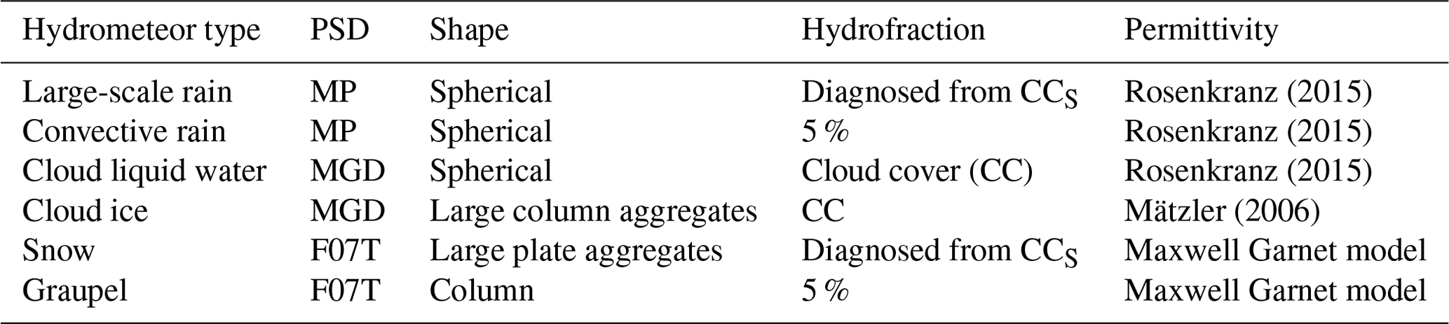
To simulate the reflectivity, bulk-scattering properties (backscattering and extinction coefficients integrated over the PSD) are stored in a lookup table as a function of temperature, frequency, and water content for each hydrometeor type (Bauer, 2001; Geer and Baordo, 2014; Geer et al., 2021). These lookup tables are generated by specifying particle shape and its associated mass–diameter relationship, PSD, and (for spheres) permittivity model for each type of hydrometeor. The operator offers the Liu database (Liu, 2008) and ARTS database (Eriksson et al., 2018) of non-spherical shapes to represent realistic frozen hydrometeor habits, which were generated using the discrete dipole approximation (DDA). For this study, the default DDA-based shapes (see Table 1) are used for snow and graupel hydrometeors as suggested by the studies of Geer (2021) and Geer et al. (2021). Similar DDA-based shapes have already been used for simulating the GPM/DPR instrument in past studies (Liao et al., 2013; Johnson et al., 2016). Spherical shapes are assumed for melted particles, including fully liquid hydrometeors (raindrops and cloud liquid water) as well as the melting layer. Mie theory is used to compute the optical properties in these cases. The densities for frozen hydrometeors are computed using the assumed mass–density relationship; for liquid hydrometeors, the density is assumed equal to 1000 kg m⁻³. The PSDs for snow and graupel hydrometeors are represented by Field et al. (2007) and a modified gamma distribution (hereafter, MGD) for ice particles. The Marshall and Palmer (1948) PSD (hereafter MP) is used for convective and large-scale rain, and a MGD is used for water cloud. It is noted that a MGD PSD is a function of four parameters (number density (N₀), $\mathit{\mu },\mathrm{\Lambda },\mathit{\gamma }$), which are different for each particle type. For cloud ice, μ=2 and $\mathrm{\Lambda }=\mathrm{2.13}\times {\mathrm{10}}^{\mathrm{5}}$ is chosen, whereas μ=0 and $\mathrm{\Lambda }=\mathrm{1}\times {\mathrm{10}}^{\mathrm{4}}$ is assigned to cloud water. N₀ is free parameter for both particles. These parameter values are taken from Geer et al. (2021). The permittivity is required for spherical particle models including the current melting-layer formulation and is computed following these models: (1) the Maxwell Garnett model extended for ellipsoid inclusions for snow and graupel, as well as the Mätzler (2006) model for ice hydrometeors down to the top of melting layer (Maxwell Garnett, 1904; Meneghini and Liao, 2000; Bohren and Battan, 1982); (2) within the melting layer, if active, the Fabry and Szyrmer (1999) model number 5 (details described in Sect. 3.1); and (3) the Rosenkranz (2015) model used for liquid water drops.

For each hydrometeor type i, the hydrometeor fraction profile f_i(R) needs to be provided to Eqs. (1), (2), and  (3). In this study, the fraction used for stratiform hydrometeors (pfrac) is derived from the cloud cover profile from the NWP model using the same formula as in the ECMWF IFS model (Park, 2018), except that the evaporation is not accounted for here. At a given level (j+1), pfrac is calculated according to Eq. (4). It is a function of the cloud cover (CC) at the current level (j+1) and the previous level (j) located above it, as well as pfrac at the jth level.

$$\begin{array}{}\text{(4)}& \begin{array}{rl}& \mathrm{pfrac}[j+\mathrm{1}]=\\ & \mathrm{1}-{\displaystyle \frac{\left(\mathrm{1}-\mathrm{pfrac}\left[j\right]\right)\left(\mathrm{1}-\max \left(\mathrm{CC}\left[j\right],\mathrm{CC}[j+\mathrm{1}]\right)\right)}{\mathrm{1}-\min \left(\mathrm{CC}\left[j\right],\mathrm{1}\times {\mathrm{10}}^{-\mathrm{6}}\right)}}\end{array}\end{array}$$

Here, CC is the cloud cover profile, and j is the height level.

The pfrac profiles computed using Eq. (4) are assigned as the hydrometeor fractions f_i(R) for stratiform snow and rain. f_i(R)=5 % is assigned to convective hydrometeor fractions for the entire profile. This study chooses 5 % because this value is being used operationally at ECMWF and Météo-France for passive microwave observations. The CC profiles are used for cloud liquid water and cloud ice water fractions (see Table 1).

For a given ARPEGE grid cell, the bulk (PSD integrated) backscattering and extinction coefficients are interpolated from the lookup tables given the temperature and in-cloud hydrometeor water content W_i(R). Then, bulk backscattering and extinction coefficients are used to compute the attenuated (AZef; Eq. 1) and unattenuated (Zef; Eq. 1 with A(R)=1) reflectivities at both Ku and Ka bands.

Rosenkranz (2015)Mätzler (2006)

Table 1 Default configuration for the six hydrometeor settings used in this study. Note that this table applies to non-melting hydrometeors only. Melting hydrometeor properties are described in Sect. 3.1.

3.1 Melting-layer parameterization of Bauer (2001)

The bulk backscattering and extinction coefficients in the melting layer depend on various factors such as permittivity, PSD, shape, phase, which can significantly alter the reflectivity computation. One of the major contributors is the permittivity which can induce significant changes in the scattering coefficients (Fabry and Szyrmer, 1999). When using a spherical model for the melting hydrometeors as done here, the permittivity and the diameter of the sphere are the main controls over the simulated scattering properties. Therefore, a major focus of this study is on an accurate representation of the permittivity within the melting layer.

The RTTOV-SCATT model includes the possibility of activating the Bauer (2001) melting scheme for snow and graupel, including the two-phase coated sphere as described in Fabry and Szyrmer (1999, their model 5). In this original parameterization, the melting-layer width is set to 1000 m, with 100 height levels ranging from the freezing level T_fl (T_fl=273 K) to the bottom of the melting layer defined by its temperature T_ml. The melting process, including the melting fraction f_m, is computed based on the model of Mitra et al. (1990).

The model starts from the relevant PSD for the completely frozen particle (e.g. Field et al., 2007) and computes the properties of these particles as they fall and melt, always using spherical particle assumptions. It should be noted that the PSDs used for snow and graupel at the top of the melting layer in version 13 of RTTOV-SCATT (e.g. Field et al., 2007 PSD) are not consistent with the ones used in the original formulation of Bauer (2001) (e.g. the Marshall–Palmer PSD). However, Geer et al. (2021) suggest that the differences between the two PSDs are not that large and that Field et al. (2007) may even have reduced the number of larger particles. Another difference with the parameterization of Bauer (2001) is that density and mass of the frozen particles are now also specified by the mass and density distributions implied by the frozen particle shape choice (see Table 1) rather than the mass–density relationship used by Bauer (2001).

At the top of the melting layer (i.e. T_fl), the permittivity properties of frozen hydrometeors are represented by the inclusion of ice in a matrix of air ([[ice], air]). As the melting process progresses, the permittivity properties change in accordance with the fraction of melted hydrometeor (f_m). Specifically, the hydrometeors are modelled as coated spheres consisting of two phases: an inner core surrounded by an outer coat. The inner core is represented by air inclusions in a matrix of ice inclusions in a matrix of water ([air,[[ice], water]]). The outer coat consists of ice inclusions within a water matrix, which is itself embedded in an air matrix ([[[ice], water], air]). In this two-phase model, the proportion of the outer coat increases as the melted hydrometeor fraction, f_m, increases. This same two-phase model has also been used for the simulation of W-band CloudSat radar reflectivity in Kollias and Albrecht (2005). Once the permittivity of the melted hydrometeor of the melted diameter D is assigned to its respective height within the melting layer, the Mie scattering calculations are performed to compute the scattering properties. They are then integrated over the number density of melted particles and averaged over the full temperature ranges (from 273 to 275 K) to provide the bulk-scattering properties. Details are given in Appendix A.

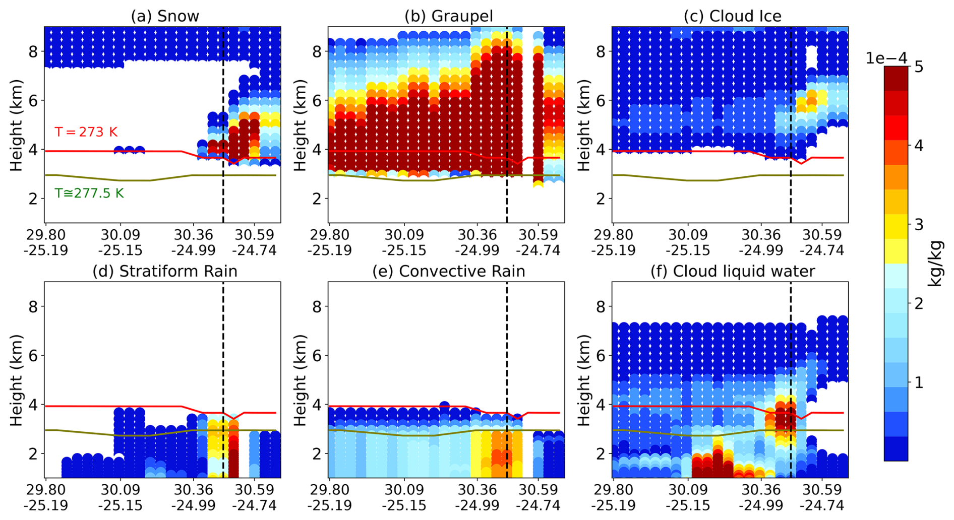
In Bauer (2001) and up to version 13.1 of RTTOV-SCATT, when the melting layer was active, the optical properties were stored in the 273 K temperature bin of the lookup tables for graupel and snow hydrometeor types, while the lower temperature bins (272 K and below) provided optical properties based on the standard frozen hydrometeor microphysical choices. However, most NWP models also include frozen hydrometeors at positive temperatures. An example from the ARPEGE global model is shown in Fig. 2, which shows a significant occurrence of graupel at warm temperature, up to 277 K. Therefore, Sect. 3.2 proposes modifications that enable a smoother and more accurate vertical representation of the melting process, in compliance with the existence of melting particles at warm temperatures.

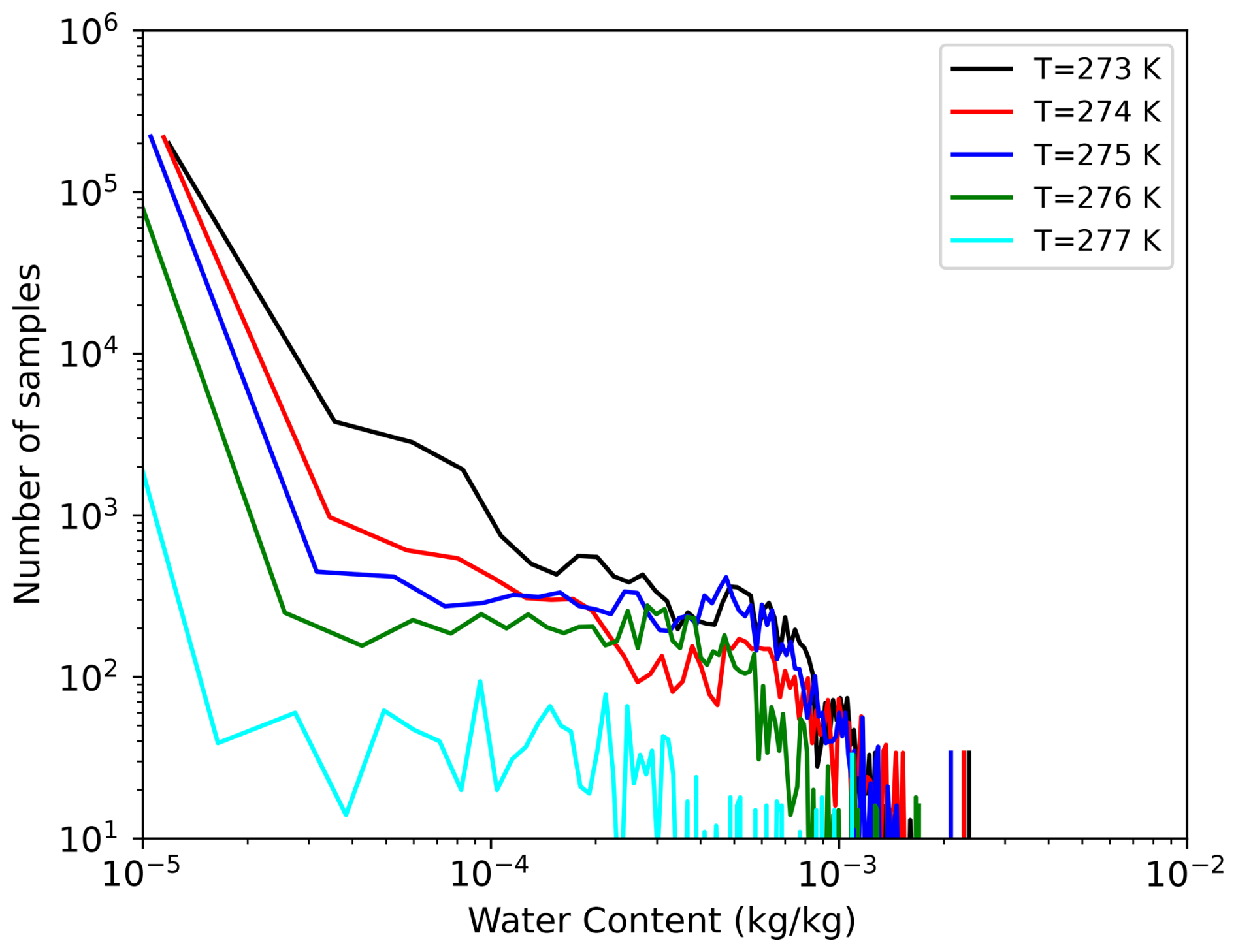
Figure 2 Distribution of graupel content at different warm temperatures from the ARPEGE global NWP model. The ARPEGE samples used here are co-located into a single GPM orbital file on 2 January 2021 (shown in Fig. 1). It is noticed that significant graupel content exists at warm temperature until 277 K and should be accounted for in melting-layer simulations.

3.2 Revised version of Bauer (2001) parameterization

First, in the revised version of the melting-layer scheme, the temperature at the bottom of the melting layer T_ml is chosen in accordance with the graupel content distribution shown in Fig. 2. Indeed, it has been observed that graupel content is significantly present until 277 K, and it is assumed that graupel is fully melted after 277 K and converted into raindrops. Therefore, T_ml is now set to 277 K for the remainder of this study. Secondly, the revised melting layer is parameterized across five sub-melting layers from 273 to 277 K in steps of 1 K, which allows us to interpolate the scattering coefficients in the lookup tables consistently with the temperature provided by the NWP model. Finally, new lookup tables of scattering coefficients including positive temperature bins for melting hydrometeors are computed in accordance with the physical processes involved in the melting layer. Further details are provided in Appendix A.

As will be seen in the following sections, the new melting layer provides a less intense but broader melting layer that is in better agreement with observations. As shown in Appendix A, this improved agreement comes partly through a reduction in backscatter that has been generated by an ad hoc scaling of the optical properties introduced by splitting the layer into five parts. This ad hoc scaling was originally unintentional, but it generated such good improvements in the melting-layer representation that it was adopted anyway.

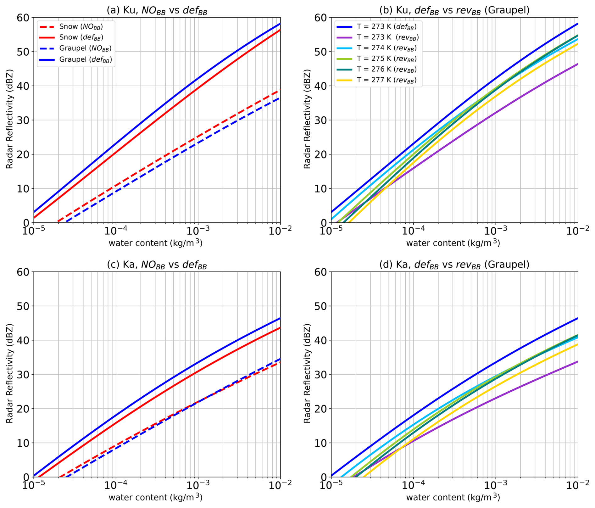
Figure 3 Radar reflectivity as a function of water content at Ku and Ka bands. (a, c) Comparison of snow and graupel reflectivities without melting layer (NO_BB) and with default Bauer parameterization (def_BB) at T=273 K. The reflectivity increases by 15 and 10 dBZ in Ku and Ka bands, respectively, after the activation of melting layer. (b, d) Graupel reflectivities are compared with the def_BB scheme (blue colour) and the revisited version of Bauer parameterization (rev_BB) at extended warm bins.

4 Impact of melting layer on reflectivity simulations

4.1 Impact of melting layer on the lookup tables

Figure 3 compares the Ku (top panels) and Ka (bottom panels) band reflectivities, derived from the backscattering coefficients of the lookup tables, for the three different scenarios: (1) no bright band (hereafter, NO_BB), (2) bright band with the original Bauer melting scheme (hereafter, def_BB), and (3) bright band with revised Bauer scheme (hereafter, rev_BB). Figure 3a and c show the comparison of radar reflectivity as a function of snow and graupel content between NO_BB and def_BB at 273 K. As expected, Fig. 3a and c show that the snow and graupel reflectivities increase by approximately 10 and 8 dB at Ku and Ka bands, respectively, with the activation of the melting layer (see the differences between different coloured lines).

Figure 3b and d compare the graupel reflectivities for the def_BB and rev_BB scenarios in both frequency bands. Consistent with the extension of the lookup table in the rev_BB scheme to warmer temperatures, the rev_BB curves are also plotted for the 274, 275, 276, and 277 K temperature bins, whereas def_BB is limited to the 273 K bin (dark blue). It is observed that the reflectivity with the rev_BB scheme is significantly reduced at 273 K (in magenta) compared to the def_BB scheme (dark blue). It is also observed that the reflectivities at warm temperatures are larger than those obtained when the particle is fully frozen (dashed blue curve in Fig. 3a), confirming that the rev_BB approach allows us to split the melting process across different temperatures within the melting layer, as shown by the different coloured lines.

Similarly, as shown in Fig. 4, extinction coefficients for snow and graupel also increase by a factor of 100, both for Ku and Ka bands, with a larger order of magnitude at Ka band. This is expected, as Ka band radars are more subject to attenuation by precipitation particles than Ku band radars.

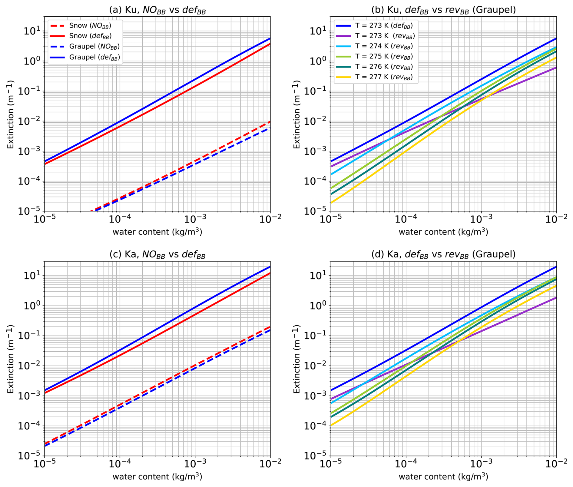
Figure 4 Similar to Fig. 3. Extinction coefficients (m⁻¹) as a function of the content are compared with the three scenarios.

Figures 3b and d and 4b and d show that the reflectivity and extinction coefficients evolve slightly differently as a function of the graupel content for sub-melting layer located at 273 K compared to the other temperature sub-melting layers (e.g. 274, 275, 276 K). For example, the reflectivity is larger (resp. smaller) at 273 K than at 277 K for a content of 10⁻⁵ kg m⁻³ (resp. 10⁻³ kg m⁻³). This non-linear behaviour is explained by the evolution of the melting process, which is different in each temperature bin, and further explained in Appendix A.

4.2 Case study

The RTTOV simulations are first performed using the default configuration (described in Table 1) for a case study mentioned in Fig. 1 and with the three scenarios (i.e. NO_BB, def_BB, and rev_BB). For the case study, the cloud profiles were selected in the area 28–32° N and 28–22° W (also shown with the grey box in Fig. 1) over the Atlantic Ocean. This case study was selected because, firstly, it is over ocean, which avoids the disparities associated with the relief in the rainy levels between neighbouring reflectivity profiles. It was also selected because of its observed bright-band signature at approximately 3.5 km of altitude. Lastly, this precipitating system is reasonably well predicted in ARPEGE, making it an ideal candidate for comparing observations with simulations made with different parameterizations of the bright band.

Figure 5 (resp. Fig. 6) compares the horizontal cross-section of observations (top panels) and simulations (in three scenarios) for the selected area at 2, 3.25, and 6 km height at Ku (resp. Ka) band. It is noticed that the observed and simulated reflectivities in the ice layers (at 6 km, right panels) are of the same order of magnitude. However, in the melting layer (at 3.25 km), the simulated reflectivities using the def_BB scheme (panel h) are overestimated by approximately 5 dB in both bands. This overestimation is slightly reduced by a factor of about 2 dB using the rev_BB scheme (panel k). Finally, in the rainy layers (at 2 km), a significant underestimation of the reflectivity is observed at Ka band when the def_BB scheme is used. This underestimation is due to a simulated bright band which is too strong, leading to an overestimation of the attenuation in the layers below the melting layer.

Figure 7 shows the time–height vertical cross-section of observed and simulated reflectivities for a cross-section around the centre of the cloud (shown by the dashed centre line in Figs. 5 and 6). In the melting region, simulated bright-band reflectivities are too strong with the def_BB scheme. With the rev_BB scheme, this overestimation is reduced by an order of approximately 5 dB. Large differences with the observations remain, which can arise by forecast errors in the input profiles or other assumptions in the forward operator (e.g. spherical particle shape, PSD, or precipitation fraction). The extremely strong bright-band signature using the def_BB scheme causes substantial attenuation in the rainy levels, especially at Ka band (panel g). Contrarily, the rev_BB scheme not only improves the bright-band reflectivity, but also reduces the attenuation affecting the reflectivities from the rainy levels. One can notice a strong rain cloud at Ku observations (Fig. 7a) probably associated with a mixture of stratiform and convective rain (near 30.09° N). However, this cloud has been shifted to the right side with higher intensity (near 30.48° N) in simulations (panel 7b–d). Such a cloud mislocation error exists in global NWP models, because it is difficult to forecast cloud and precipitation at the right location with the right intensity (Fabry and Sun, 2010). The low precipitation fraction f_i(R) (5 %) used for convective hydrometeors is also one factor for the overestimation. As stated in Eqs. (1) and (2), the in-cloud water content is normalized by f_i(R); this causes the change in shape of the PSD. A sensitivity study to the precipitation fraction is shown in Appendix B for the case study.

A single profile with an observed bright-band signature is also diagnosed from the experimental cloud (the dashed black line in Fig. 7 corresponds to its location) and is shown in Fig. 8. The observed profile is depicted in grey, and the attenuated (panels a, b, e, f) and corrected (panels c, d, g, h) simulations under three scenarios are depicted by the dotted, dash-dotted, and solid lines, respectively. The Ku band simulated profiles indicate that the def_BB scheme overestimates the bright-band reflectivity that results in large observed minus simulated reflectivities (or first-guess (FG) departure) of approximately −15 dB maxima. However, the rev_BB scheme produces a smoother transition of the reflectivities within the melting layer and is found to be in better agreement with the observations with smaller FG departure ($\sim -\mathrm{9}$ dB maxima). One can notice that both AZef and Zef simulations are overestimated in the rainy levels at Ku band. This could be due to the model (overestimation of the rain) or to a misrepresentation of the rain within the forward operator (e.g. precipitation fraction and/or PSDs). Interestingly, the overestimation is larger (panels a, b) when the bright band is not simulated. There is an artificial improvement of the bias when the bright-band signal is too strong, which explains why def_BB is better in the rainy levels. Indeed, a large bright-band signal increases the extinction coefficient, which significantly increases the attenuation in the rainy levels. On the other hand, Zef at Ka band shows the opposite behaviour (i.e. underestimation) in the rainy levels. This may be due to strong attenuation with rain particles at Ka band. Furthermore, the profile of simulated attenuated reflectivity AZef indicates a very high underestimation of the rain reflectivity (∼10 dB) by the def_BB scheme, followed by slightly reduced underestimation (∼3 dB) using the rev_BB scheme and almost negligible with NO_BB in comparison to observed reflectivity. Results from a case study using a small sample size show the positive benefits of the rev_BB scheme in the melting levels as well as in the rainy levels at both Ku and Ka band frequencies.

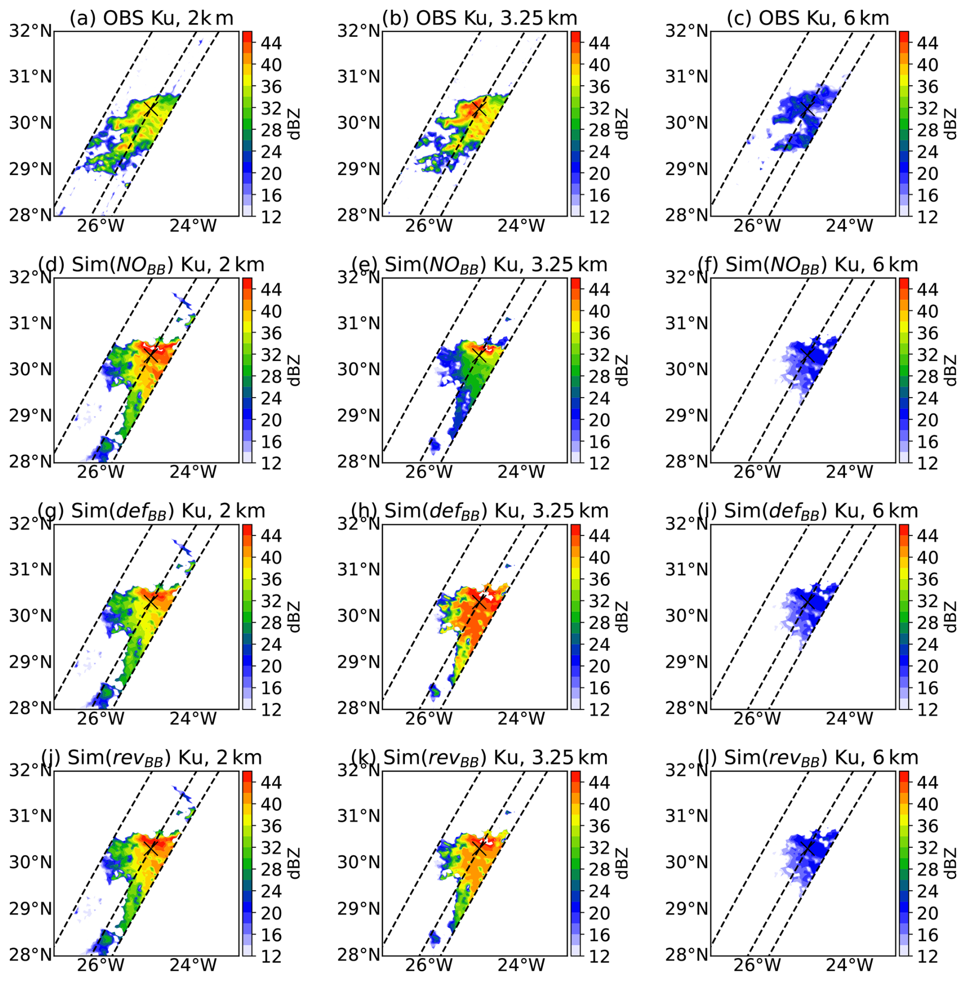
Figure 5 Horizontal cross-section over the selected area at 2, 3.5, and 6 km heights for Ku band. The top panels (a–c) show the observations, panels (d–f) show the simulation without bright band (NO_BB), panels (g–i) show the simulated reflectivities with bright band using the def_BB scheme, and panels (j–l) show the simulations with the rev_BB scheme. The central dashed line represents the three-dimensional cross-section, and the cross mark represents the location of the single profile which is used for diagnosis later in this section.

Figure 6 Same as Fig. 5 but for the Ka band.

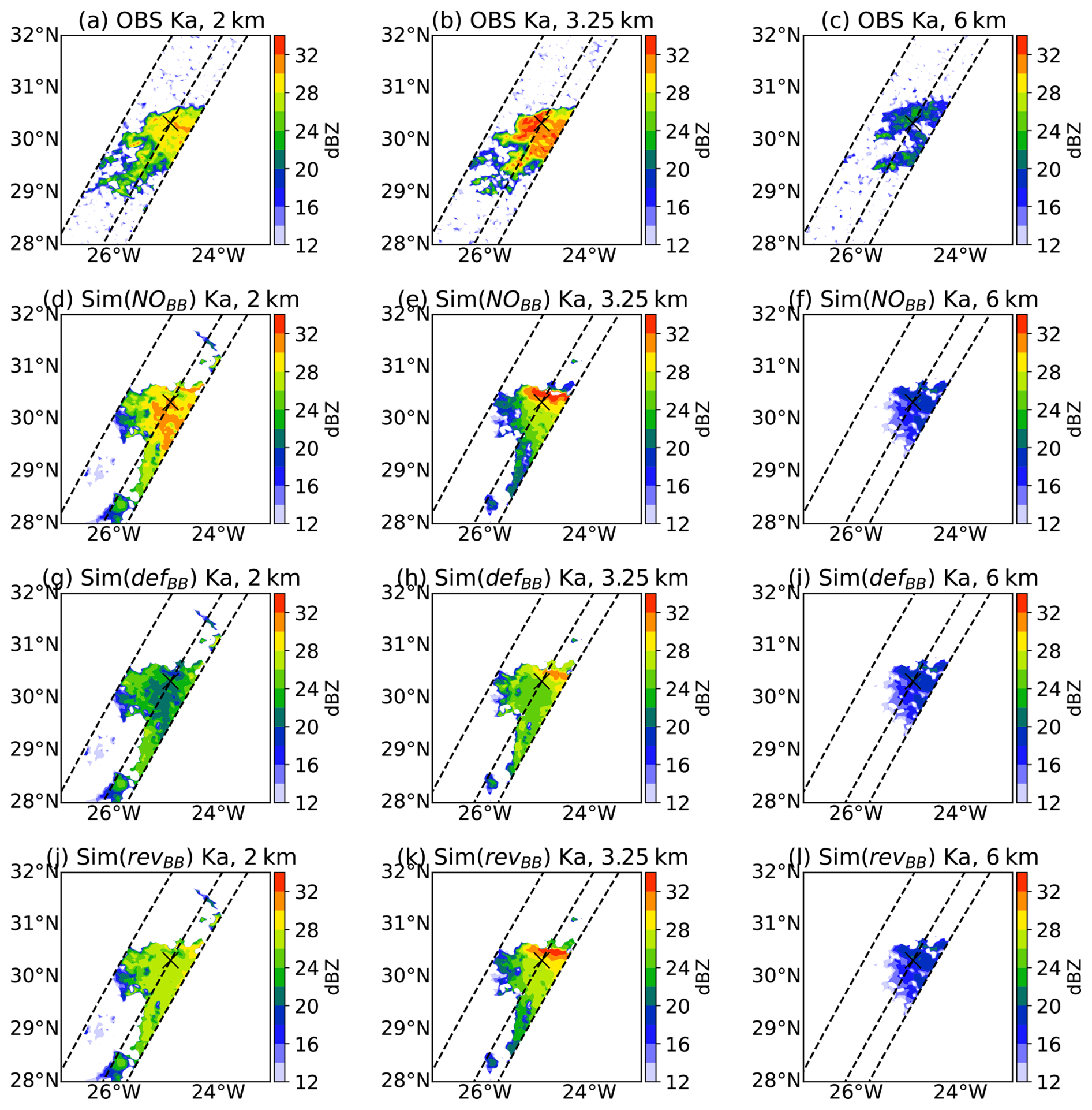
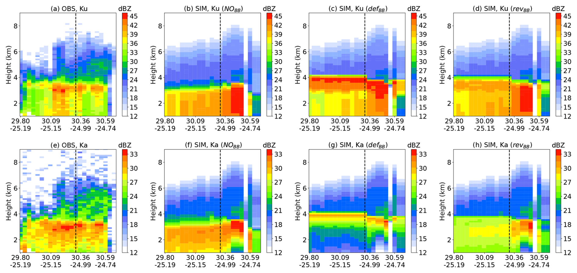
Figure 7 (a, e) Vertical cross-section of the selected cloud in the observations and (b–d and f–h) simulations with three scenarios as mentioned above: NO_BB, def_BB, and rev_BB configurations for Ku and Ka bands, respectively. The dashed black line is the single profile used for the diagnosis.

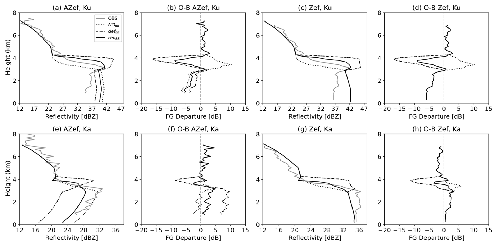
Figure 8 (a, e) An attenuated reflectivity (AZef) and (c, g) unattenuated reflectivity (Zef) profile is diagnosed from the experimental cloud at Ku (a–d) and Ka band (e–h) and compared with RTTOV simulated profile under three different scenarios. The first-guess departure at both frequencies is also shown in panels (b, f) and (d, h) for AZef and Zef, respectively.

4.3 Statistical assessment over a 1-month period for two seasons

Section 4.2 demonstrated the positive impact of rev_BB on a case study. The impact is now shown over a longer period. This study performed simulations of DPR reflectivities for a 1-month period of two seasons, i.e. June 2020 and January 2021, using the NO_BB, def_BB, and rev_BB configurations. Only samples where both observed and simulated attenuated reflectivities are above the radar sensitivity of 12 dBZ are considered for computing the first-guess departure statistics. Figures 9 and 10 show the vertical distribution of FG departure statistics with statistical hypothesis tests (Levene's and Welch's t tests). The standard deviation is shown in the leftmost panels; bias is shown in the right panels in the NH region (23.43 to 60° N: top panel), the tropics (23.43° S to 23.43° N: middle panel), and the SH region (60° S to 23.43° S: bottom panel) at Ku and Ka bands, respectively. The Levene (Levene, 1960) and Welch t tests (Zimmerman and Zumbo, 1993) are used to test the equality of variances and means, respectively. These hypothesis tests are demonstrated for two cases at each height level. The null hypothesis for the Levene test is “the standard deviations are equal”. The first case, denoted as Case 1, is to test the def_BB scheme against the NO_BB (without bright band) one to show the impact of the activation of the bright band. The second case, denoted Case 2 is to test the rev_BB scheme against def_BB to check whether the revised scheme degrades or improves the FG departure statistics. If the p value is less than 0.05, the null hypothesis is rejected, which means that the standard deviations are statistically significantly different. The differences are represented by red and blue triangles. For example (Fig. 9b, Case 1), the blue colour represents those height levels where the standard deviation of the def_BB scheme samples are less than the standard deviation of NO_BB (indicating improvement) and the reverse for the red colour (indicating degradation). The grey colour represents levels of neutral impact (equal standard deviations). Similarly, the Welch t test is performed but for the mean.

It is observed that the standard deviations and biases of FG departure statistics with the revised BB (rev_BB) scheme are improved in the three domains compared to the ones with the default BB (def_BB) scheme in the melting zone at Ku band, even though, to a lesser extent, the impact is also positive at Ka band in the melting layer. From the contoured frequency by altitude diagrams (CFADs) that are shown in Sect. 5.3 (see Figs. 14 to 17), it is clear that the revised parameterization rev_BB provides a more realistic simulation of the bright band in terms of reflectivity profiles compared to both NO_BB and def_BB. The error characteristics in Fig. 9 are larger when the def_BB scheme is used, followed by the rev_BB scheme compared to the ones without any bright-band (NO_BB) simulations. One possible explanation for the larger standard deviation despite more realistic simulations, compared to the NO_BB scheme, is that activating the melting layer diminishes the overall smoothness of simulated profiles. This can lead to spurious degradations of the FG departure statistics. This behaviour can somehow be linked to a double-penalty effect in the vertical, more known on the horizontal when performing precipitation verification (Ebert et al., 2007; Roberts and Lean, 2008). A good example is shown in Sect. 4.2 with the single profile shown in Fig. 8. The freezing-level height is at approximately 3.5 km in the observations and approximately 4.0 km in the model. Because of the shift of the freezing-level height between observation and NWP model, the FG departure is overestimated just below the freezing level (occurs first either in observation or simulation). Then, the overestimation continues until the bottom of the melting layer (occurs lastly either in observation or simulation). This is called a double-penalty issue and degrades the forecast scores (Cintineo et al., 2014). Without any simulation of the bright band (NO_BB scheme), there is only one penalty located at the location of the observed BB, which explains the smaller FG departure statistics.

The significance test for Case 1 (e.g. def_BB versus NO_BB) reveals that high magnitudes of standard deviation and bias due to the bright band are statistically significant (shown by red triangles). However, in the tropics there is significant improvement in error over the rainy levels (especially at Ka band). This is due to a bright band that is too strong, which significantly increases the attenuation within the bright band and, in turn, reduces the overestimation artificially in the rainy levels. However, the opposite is true for Case 2 (e.g. rev_BB versus def_BB), which indicates that errors are better represented by rev_BB in comparison to def_BB and are statistically significant. Figure 9d and l show that bias values with rev_BB are suddenly larger than the def_BB scheme for the ice levels of the cloud (∼5–6 km altitude) and vice versa for lower levels.

One important feature that can also be noted in Fig. 9 is the negative bias in the rainy levels, which can be quite large, especially in the tropics. Indeed, the bias magnitude is only in the 0–5 dB range in the Northern Hemisphere and Southern Hemisphere (top and bottom panels) but can reach approximately −15 dB in the tropics (middle panels). The bias could arise from several sources, including from the physical parameterization of the model for tropical convection but also from a misrepresentation of convective rainfall in the forward operator. This study indeed assumes 5 % for convective hydrometeors precipitation fraction. As mentioned in Sect. 4.2 and in Appendix B, a small precipitation fraction can drastically increase the reflectivity, which results in a strong overestimation of the reflectivity. This needs to be investigated in a future study. Another assumption is the particle size distributions (PSDs) used for rain. This study uses the Marshall and Palmer PSD for both stratiform and convective rain, but other PSDs could be tested as well. For example, as done by Fielding and Janisková (2020) for the simulation of CloudSat-CPR reflectivity in the ZmVar forward operator, the Illingworth and Blackman (2002) PSD could be tested for convective rain. For stratiform rain, the Abel and Boutle (2012) PSD, which is the one used in the microphysical scheme of ARPEGE, could be used to have consistent assumptions in the forward operator and in the model.

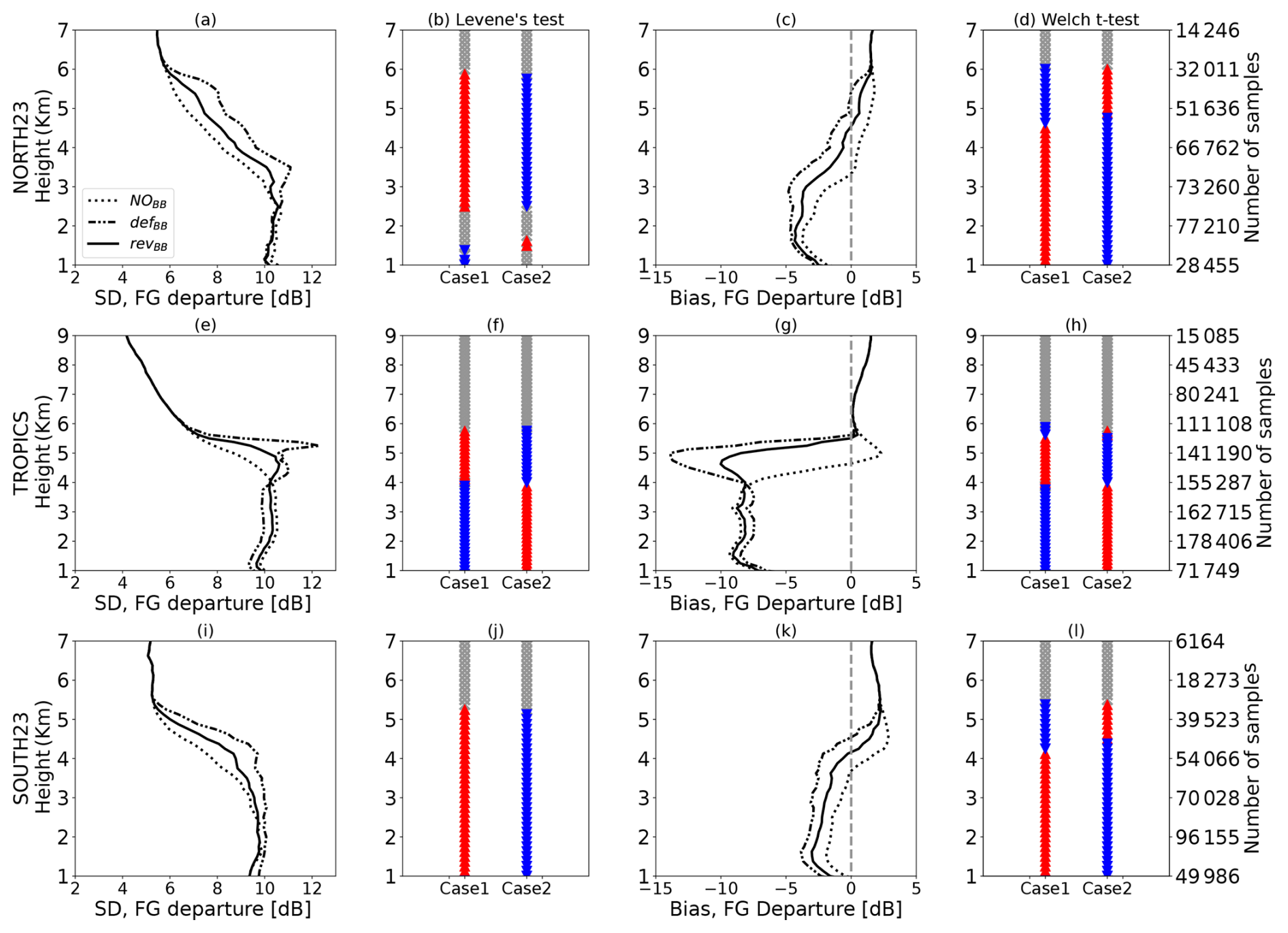
Figure 9 Standard deviation and bias of observed-minus-simulated attenuated reflectivities (or first-guess departures) are shown for combined samples of 2 different months (June 2020 and January 2021) at Ku band in (a–d) the Northern Hemisphere, (e–h) the tropics, and (i–l) the Southern Hemisphere. Results with NO_BB, def_BB, and rev_BB schemes are compared. The statistical hypothesis tests are represented by the coloured triangles to assess the equality of standard deviation (Levene's test) and mean (Welch's t test). Case 1 illustrates the impact of activating bright band using the def_BB scheme with reference to NO_BB, whereas Case 2 shows the assessment of the rev_BB scheme in comparison to the def_BB scheme. For Case 2, blue (red) triangles indicate that the standard deviation of the rev_BB scheme samples are smaller (larger) than the standard deviation of def_BB, which indicates an improvement (degradation) of the rev_BB scheme. Grey colours represent levels of neutral impact (equal standard deviations). Note that the same behaviour is obtained with separated 1-month samples.

Figure 10 Similar to Fig. 9 but for the Ka band

5 Application of the melting layer for precipitation classification

An application of the combined use of Ku and Ka band attenuated reflectivities is the use of the dual-frequency ratio (DFR = ZKu − ZKa) to classify precipitation into three precipitation categories, i.e. stratiform, convective, and transition (Iguchi et al., 2010; Awaka et al., 2016). If a bright band and rain are detected, the category of a profile will be decided in accordance with the variation of the DFR profile. In this study, the same DFR classification strategy (Awaka et al., 2016) as the one used in the level 2 product of GPM DPR observations is applied to ARPEGE simulations. The methodology is described in Sect. 5.1, followed by a validation on the same case study as the one used in the Sect. 4.2 and on the full period of study as well.

5.1 Methodology

Figure 11 shows the flow diagram of the methodology adopted for this study (Awaka et al., 2016). In accordance with the vertical profiles of temperature and simulated DFR, the first step is to check if there is a melting region for this profile. In particular, the melting region is detected if the temperature (T) is between 273 and 277.5 K and if a DFR is larger than 0.0 dB. After detecting the bright band, the maximum of DFR is searched above 1 km and below 2 km from the freezing-level height (height at 273 K, denoted as point A) within the melting zone only. If this criterion is satisfied, then the maximum DFR value is identified (hereafter, DFR_max) and named as point B.

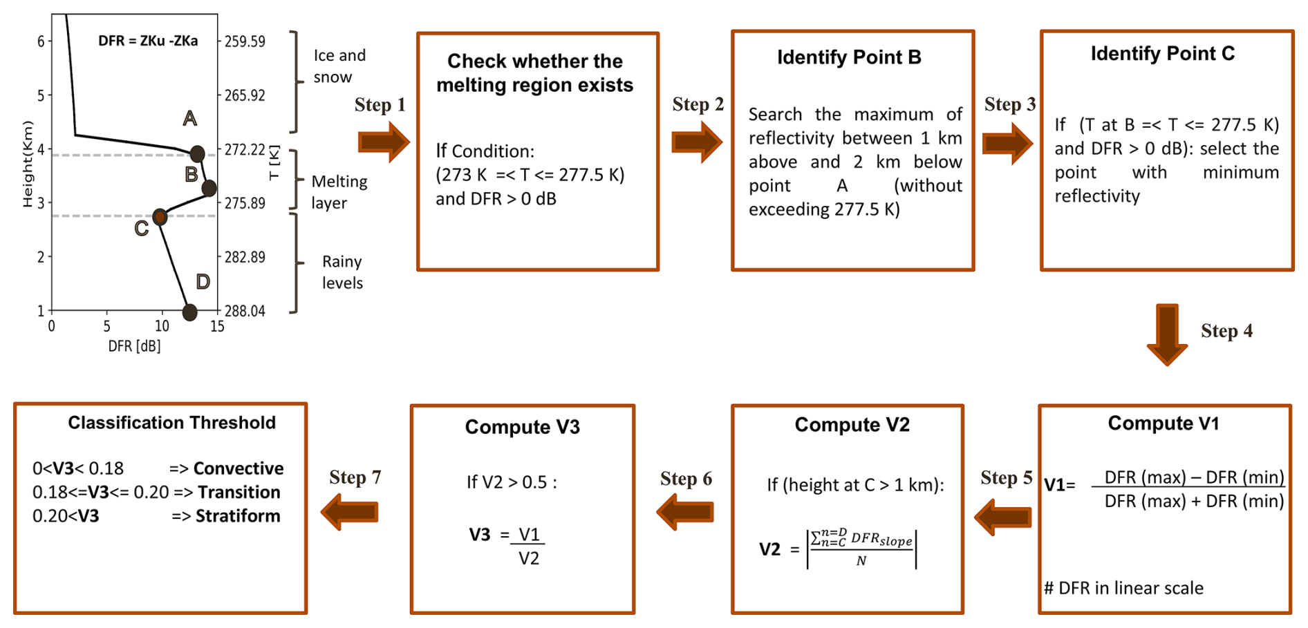
Figure 11 Methodology adopted for precipitation type classification using the dual-frequency ratio method, which is based on the detection of the melting layer in the simulations.

The next step is to find the bottom of the melting layer, denoted by point C. This is done by searching for the minimum value of DFR (hereafter, DFR_min) below the melting layer. The DFR_max and DFR_min are converted into a linear scale in order to compute the different indexes used for the classification. In particular, a V1 index is defined using DFR_max and DFR_min values as shown in the following Eq. (5). The larger the V1 value, the larger the chances to categorize the column as stratiform.

$$\begin{array}{}\text{(5)}& V\mathrm{1}={\displaystyle \frac{{\mathrm{DFR}}_{\max }-{\mathrm{DFR}}_{\min }}{{\mathrm{DFR}}_{\max }+{\mathrm{DFR}}_{\min }}}\end{array}$$

Here, DFR_max and DFR_min are in a linear scale.

The next step is to check if rain exists or not through the computation of the V2 index. If point C is above an altitude of 1 km, then the second index V2 is computed by extracting all height and DFR values from point C to D (bottom most of the profile). The V2 index (dB km⁻¹)) is the absolute value of mean slope of DFR from C to D. It is calculated according to Eq. (6):

$$\begin{array}{}\text{(6)}& V\mathrm{2}=\left|{\displaystyle \frac{{\sum }_{n=C}^{n=D}\mathrm{DFR}\mathrm{slope}}{N}}\right|.\end{array}$$

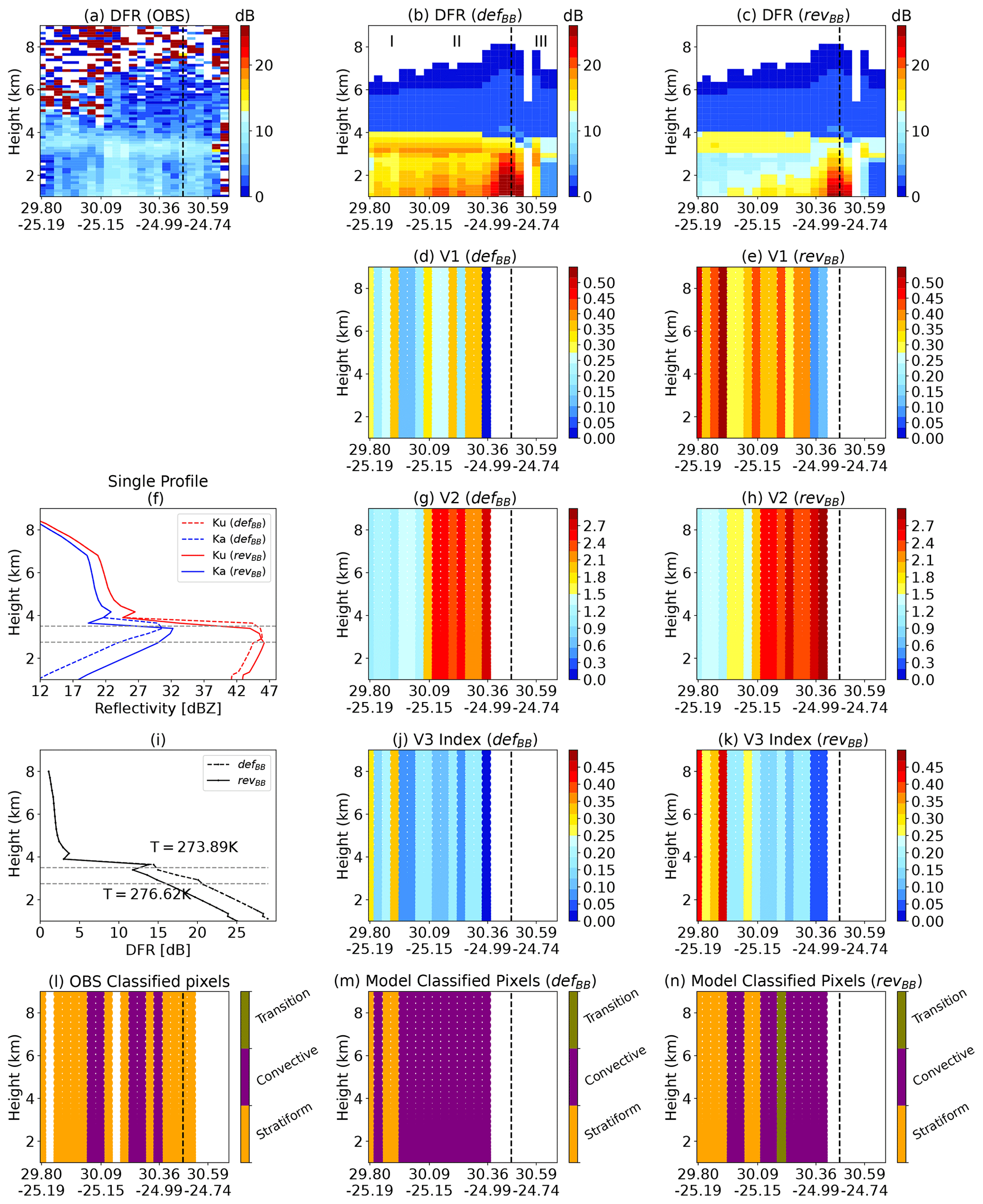
Figure 12 (a–c) Vertical cross-section of DFR for the case study in observations and model simulations using the def_BB and rev_BB schemes, respectively. Panels (d, g, j) are the V1, V2, and V3 parameters corresponding to the simulations performed using the def_BB scheme; similarly, panels (e, h, k) are for the rev_BB scheme. Panels (l, m, n) are the classified pixels which correspond to the observations, the def_BB scheme, and the rev_BB scheme, respectively. The dashed black horizontal line in panels (f) and (i) represents the temperature of top (T=273.89 K) and bottom (T=276.2 K) of the melting layer for the given profile. Note that we do not perform classification on observations, as this is already performed in the level 2 products. Instead, we used the classification flag to separate out the DFR-classified pixels for comparison. The profile shown in the middle-left side corresponds to the dashed black line in all panels.

The larger the V2 value, the larger the probability for convective precipitation classification. If V2 is less than 0.5 dB km⁻¹, then the DFR classification algorithm is not used as followed in the past literature (Awaka et al., 2016; Iguchi et al., 2010). Note that both V1 and V2 are normalized values and are independent of height and depth of melting layer (Iguchi et al., 2010).

Figure 13 Vertical structure of hydrometeors following the cross-section in Fig. 12. The red and green lines correspond to the 273 and 277.5 K temperature levels, respectively, which correspond to the vertical levels in which frozen particles are allowed to melt (see Sect. 3.2).

The last step is to calculate the ratio of V1 and V2 to define an effective parameter V3 ($=\frac{V\mathrm{1}}{V\mathrm{2}}$) for the classification. The thresholds used here for the classification (convective: $\mathrm{0}<V\mathrm{3}<\mathrm{0.18}$; transition: $\mathrm{0.18}<=V\mathrm{3}<=\mathrm{0.2}$; stratiform: 0.2<V3) are the same as the ones given in the GPM algorithm theoretical basis document (ATBD) and also used in the past studies for the classification of GPM observations (Awaka et al., 2016). These threshold values have been computed from extensive statistical analysis of GPM DPR profiles and airborne radar profiles (Iguchi et al., 2010).

5.2 Validation for the case study

The DFR algorithm is first applied to the case study (same one as previously shown in Sect. 4.2). It has been already discussed in the previous sections how the rev_BB scheme allows us to have more realistic bright-band simulations compared with the observations. As an extra validation step, this study aims at showing whether the revised melting-layer parameterization can be used for classifying stratiform/convective precipitation with a standard method. In this study, the classification algorithm is first applied to simulations using both bright-band parameterization schemes and then compared with the classification of the observations dataset. It should be noted that only DFR-algorithm-classified pixels in the observation dataset are compared. In Fig. 12, panels (a–c) show the vertical cross-section of DFR (observation as well as models), panels (d–e) show the V1 parameter, (g–h) show the V2 parameter, and (j–k) show the V3 parameter for the def_BB scheme and the rev_BB scheme, respectively. Panels (l) to (n) show the classified pixels in the observations, in the simulations with the def_BB scheme and with the rev_BB scheme, respectively. For ease of interpretation, markers I, II, and III are shown in panel (b) to represent different precipitating zones of the time–height cross-section.

Overall, the pattern in Fig. 12b and c is in good agreement with the observations (Fig. 12a). The V1 parameter in both schemes shows that pixels in region I have higher values than region II. On the contrary, the V2 parameter shows the opposite pattern but is in accordance with the algorithm. One can observe that the magnitudes of V1 and V2 differ with the change in bright-band scheme. Finally, the deciding parameter (i.e. V3) enlarges the differences and leads to categorize region I as stratiform precipitation and region II as convective precipitation. However, the majority of region III pixels have no classes. The reason could be associated with high DFR values in the rainy levels. The DFR profile with the def_BB scheme has not only a bright band that is too strong, but also high DFR values in the rainy levels because of high attenuation at Ka band. In general, increased attenuation results in lower rain reflectivity and higher DFR values (Kobayashi et al., 2021). One example of a high DFR profile can be seen in the Fig. 12f and i. The dashed and solid lines correspond to the def_BB and rev_BB schemes, respectively. As a result, there are no minima in the DFR (refer the step 3 in Fig. 11) at the starting point of rainy region, which ends the algorithm and results in no classification. Therefore, more gaps can be seen with the def_BB scheme as compared to the rev_BB scheme.

To validate the simulated DFR classification algorithm, which mirrors the observed classification algorithm, the classification results are compared with model variables. The latitude–height cross-sections of hydrometeors are shown in Fig. 13. Both stratiform and convective contents are smaller in region I, slightly larger in region II, and significantly larger in region III. The large DFR in rainy levels in Fig. 12b corresponds to an area with model-predicted stratiform and convective rain together. Overall, the hydrometeor time–height cross-section is in reasonably good agreement with the classification results.

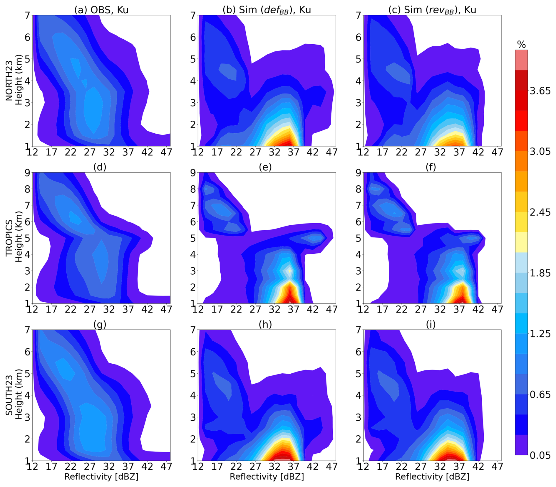
Figure 14 Normalized contoured frequency by altitude diagram (CFAD) of Ku band for stratiform pixels for the 2-month period (June 2020 and January 2021) over the Northern Hemispheres (a, b, c), the tropics (d, e, f), and the Southern Hemisphere (g, h, i). The colour bar represents the percentage of pixels in 2 dBZ × 0.5 km bin.

5.3 Global analysis over the 2-month period

The classification is now applied to a larger number of samples for 2 different months (June 2020 and January 2021) using def_BB and rev_BB schemes. Figures 14 and 15 show the normalized contoured frequency by altitude diagram (CFAD) of the attenuated reflectivity profiles classified as stratiform in the three geographical domains at Ku and Ka bands, respectively. The left column is observation, and middle and right columns are the simulations using the def_BB and rev_BB schemes, respectively. The bin size is 2 dBZ × 0.5 km. The vertical distribution of simulated reflectivities are in reasonable agreement with observations at both bands. However, the occurrence of simulated reflectivities are lower over the ice region and significantly higher over the rainy levels in all geographical domains as compared to the observations. It can be seen that the rain reflectivities are 5 dB larger in the simulations than in the observations at Ku band. This reveals the model bias due to microphysical assumptions in the ARPEGE global model that leads to overestimated rainfall. It could also be attributed to a misrepresentation (e.g. precipitation fraction) of the large-scale rain in the forward operator. These discrepancies are similar in the three geographical domains, indicating that the differences in horizontal resolution across the globe with the ARPEGE stretched grid have a secondary effect with respect to other model biases. In the tropics, it is worth noting that the bright-band peak with the rev_BB scheme (≈ 42 dBZ at an altitude of 5 km) is in better agreement with the observations (≈ 43 dBZ), as compared with the def_BB scheme which overestimates the peak (≈ 46 dBZ).

Similarly, Figs. 16 and  17 show the CFAD for convective precipitation columns. The vertical pattern of convective precipitation is in reasonably good agreement with the observations at Ka band, even though, to a lesser extent, a good match with the observations is also observed at Ku band. The observed reflectivities at Ku band are in the ∼17–24 dBZ range from the cloud top to the surface over NH and SH regions due to the dominance of shallow convection. However, tropical regions are well known for the presence of deep convective systems which lead to strong reflectivities of the order of ∼35–40 dBZ (Liu and Zipser, 2015; Liu and Liu, 2016). The simulated reflectivities over ice regions are well matched, but rainy levels are significantly larger (∼ up to 15–18 dB) over the NH and SH regions and approximately up to 5 dB in the tropics. The overestimation of rain reflectivity up to 5 dB is probably associated with the smaller value of convective precipitation fractions in the forward operator (5 %) (see Appendix B). One can observe the negative slopes in the lower levels at Ka band (Fig. 17) but not at Ku band (Fig. 16). This is because the Ku band radar can easily penetrate the medium-to-large frozen particles and go deeply into the rainy levels (∼1–2 km), whereas the signal at Ka band is more attenuated by these particles.

Figure 15 Same as Fig. 14 but for the Ka band

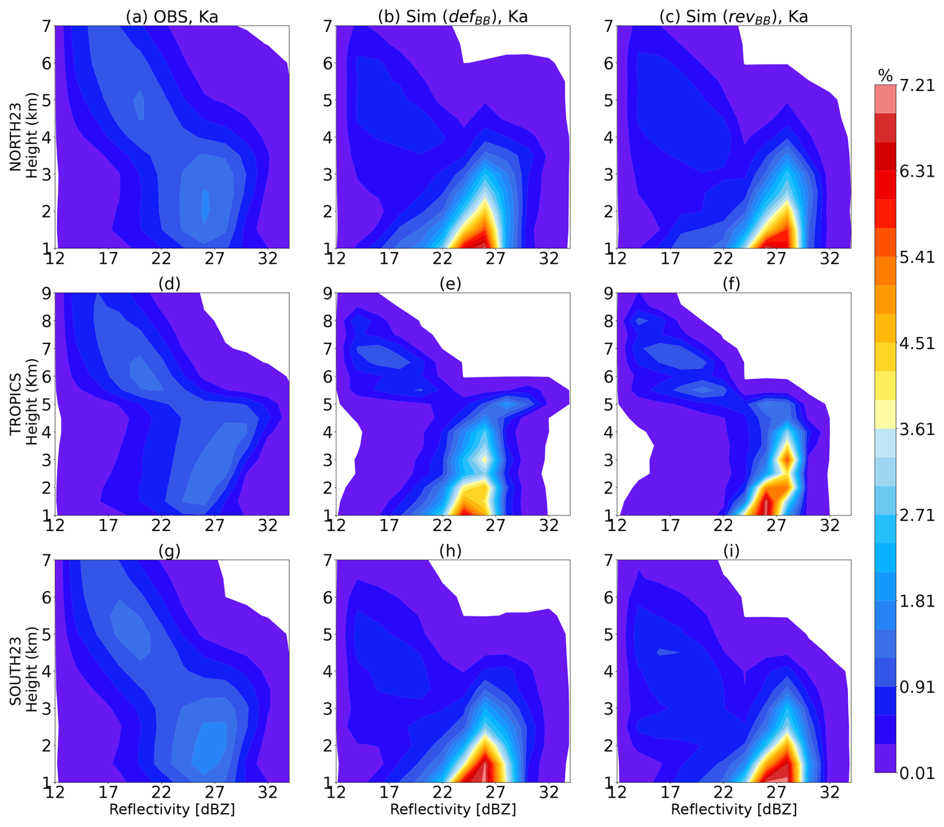
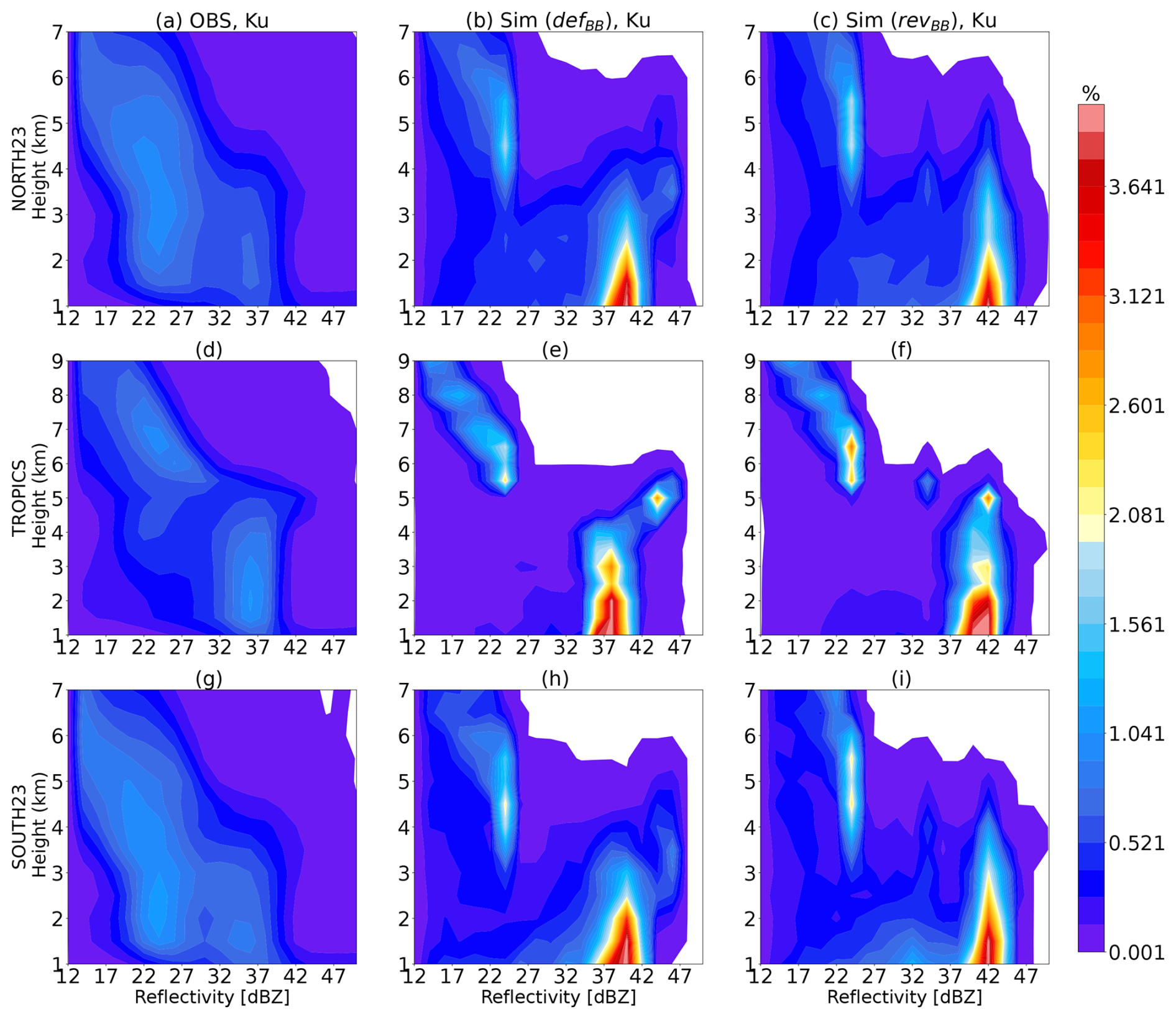
Figure 16 Normalized CFAD of Ku band for convective pixels for the 2-month period (June 2020 and January 2021) over the Northern Hemisphere (a–c), the tropics (d–f), and the Southern Hemisphere (g–i).

Figure 17 Same as Fig. 16 but for the Ka band

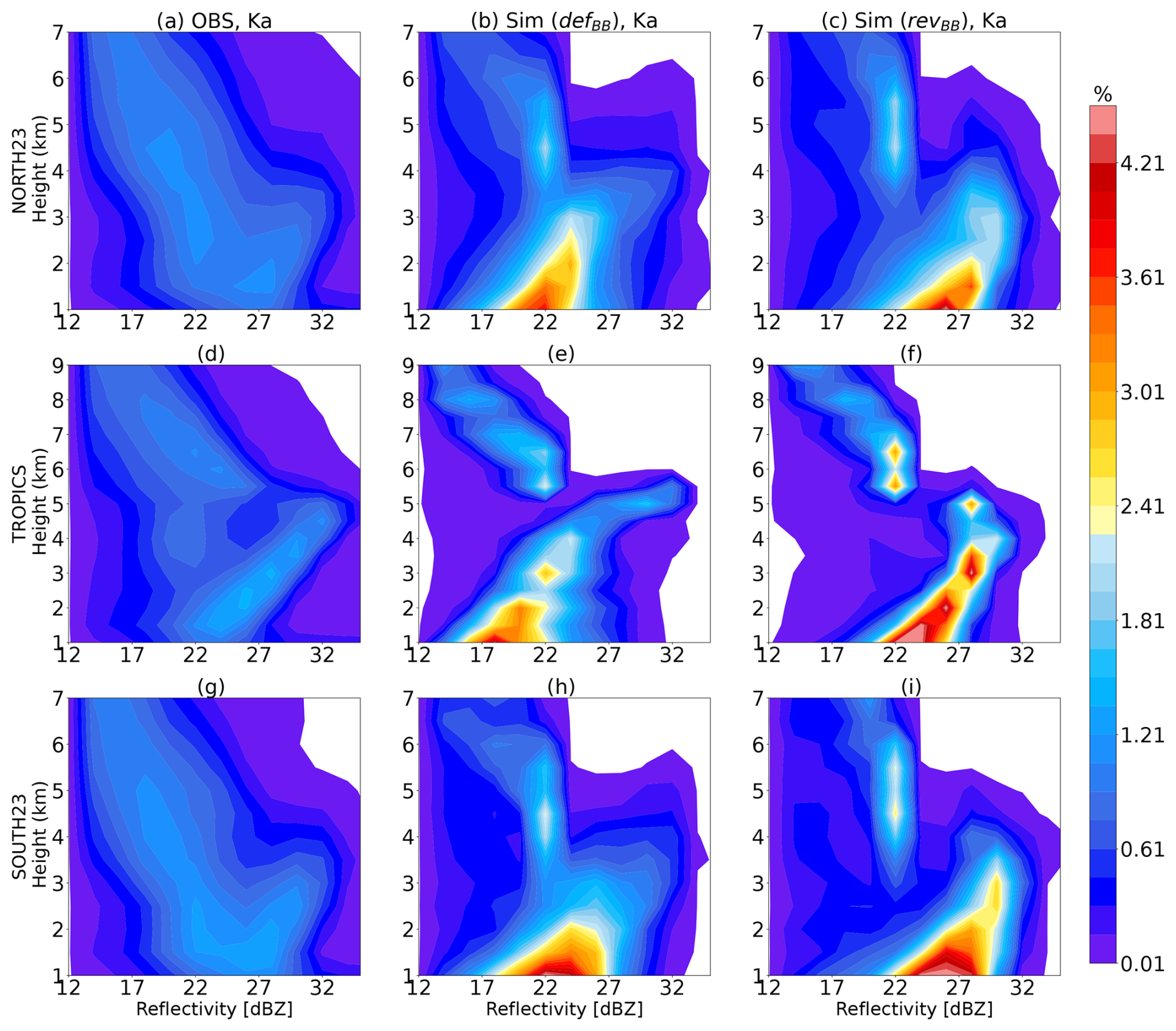
Table 2 Percentage of classified pixels in observations and model. The N, T, and S symbols denote Northern Hemisphere, the tropics, and the Southern Hemisphere regions.

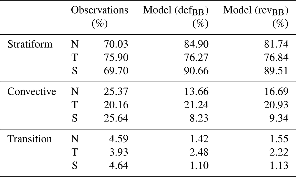
Table 2 shows the percentage of classified pixels in the observations and ARPEGE NWP model using def_BB and rev_BB schemes over the NH, the tropics, and the SH regions. In the NH region, the def_BB scheme overestimates (resp. underestimates) the number of stratiform (resp. convective) profiles by ∼13 %–14 %. However, the rev_BB scheme decreases (increases) the number of stratiform (convective) profiles by ∼3 % in comparison to the def_BB scheme and tends to move closer to the observations. A similar tendency is observed in the SH. Over the tropical region, both schemes show a good match with the observations for both stratiform and convective precipitation. In summary, the rev_BB scheme, as compared to the def_BB scheme, shows a slight improvement in the detection of the occurrence of stratiform and convective profiles over the NH region. The percentage of transition profiles is very small, which does not lead to any robust conclusions.

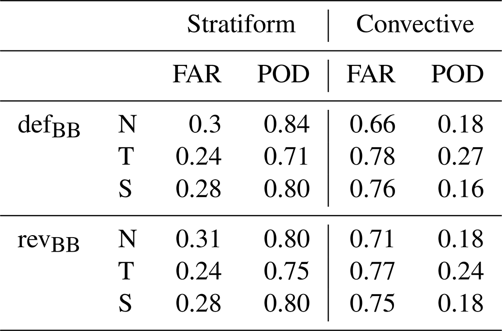
Table 3 shows the false alarm ratio (FAR) and probability of detection (POD) values using the def_BB and rev_BB schemes in the three regions (see details in Appendix C). It can be seen that FAR is low and POD is high for stratiform precipitation and vice versa for convective precipitation classification. This could be due to the difficulties in precisely locating the convective precipitation in the ARPEGE model, which has a smaller horizontal extent than stratiform precipitation. One can notice that FAR remains the same with both melting schemes for both stratiform and convective events. In the case of a stratiform event, the rev_BB scheme decreases (increases) the POD from 0.84 (0.71) to 0.80 (0.75) over NH and tropical regions, but the impact in the Southern Hemisphere is much less important. However, the impact is reversed for convective events. The rev_BB scheme improves the classification of stratiform precipitation columns over the tropics, as well as the classification of convective precipitation over the Southern Hemisphere. Overall, both bright-band schemes show great potential in precipitation classification for both qualitative and quantitative assessment.

It should be noted that one of the limitations of the classification algorithm is that multiple scattering effects are not simulated in the forward operator. In the presence of a deep convective core (mostly in the tropics), multiple scattering effects impact the reflectivity simulations and should be accounted for in the dual-frequency retrieval algorithm (Battaglia et al., 2015). This study assumes only single-scattering effects, which could be one deficiency of the DFR algorithm to detect convective columns in the model space.

Table 3 Probability of detection (POD) and false alarm ratio (FAR) corresponding to the def_BB and rev_BB schemes over the three regions, respectively.

6 Conclusions and perspectives

The present study assesses the simulations of GPM/DPR reflectivities within the RTTOV-SCATT model, providing a first validation of the reflectivity scheme that was introduced with RTTOV v13.1. Further, for the first time the optional melting-layer parameterization provided with RTTOV is validated in the context of active rather than passive measurements (Bauer, 2001). The ARPEGE global NWP model 6 h forecasts are used as input to the forward operator. Simulations are made with and without the melting layer and compared with observations. The RTTOV model offers the Bauer (2001) melting-layer parameterization scheme for microwave radiometers and radars. This parameterization had never been tested for GPM/DPR and in practice does not appear to fit observations well. Hence, the current study proposed a revised version of the Bauer scheme (rev_BB) to provide a smoother and more accurate vertical representation of the melting process in the bright band.

The design of the revised bright band extends the melting layer to 277 K rather than just to 275 K, based on modelling results. The change also introduces an ad hoc scaling factor that helps reduce backscatter and improves the fit to the observations. A potential limitation of the scheme is that the results are based on Mie spheres, while a more physical non-spherical modelling of melting particles is being developed (e.g. Johnson et al., 2016). The next step would be to further enhance this melting-layer formulation with one that follows a stronger physical basis, including modelling of non-spherical particles. That may be a challenging task and depends on ongoing developments in non-spherical modelling, so it is left for future work.

As a first step of evaluation, results were generated for a case study within the single orbital file on 2 January 2021 with and without a representation of the melting layer. Results indicate that the simulated reflectivities at the freezing level with the rev_BB scheme both at Ku and Ka bands are closer to the observations (by an order of approximately 5 dB) compared to either the original def_BB scheme or no bright band. The simulations were performed for 1-month periods in two seasons (June 2020 and January 2021). The statistical assessment shows significant improvement in the FG departure statistics around the melting-layer region using the rev_BB scheme. This positive improvement is particularly evidenced at Ku band. However, below the melting layers, the rev_BB scheme can lead to an artificial degradation of the statistics, which is probably due to a tendency of ARPEGE to produce a number of convective hydrometeors that is too large or due to the misrepresentation of convective hydrometeors within RTTOV-SCATT. The rev_BB scheme is available in RTTOV v13.2 (released on November 2022), and the def_BB scheme was discontinued.

As an indirect validation method, this study applied the methodology for precipitation classification into three categories, i.e. stratiform, convective, and transition, using the dual-frequency ratio (DFR, Ku–Ka) method for simulations. The performance for case studies is in reasonable agreement with observations and also in accordance with the vertical distribution of hydrometeors produced by the ARPEGE NWP model. Overall, the rev_BB scheme shows slightly better potential than the def_BB scheme in classifying a model column into a given precipitation category. Indeed, the number of classified pixels in each category is in better agreement with the observations (e.g. 25.37 % in the NH for convective precipitation) when the simulations are performed with the rev_BB (e.g. 16.69 %) than with the def_BB (13.66 %) scheme. Finally, CFADs of rev_BB classified pixels also reveal the model bias in all hemispheres and show significant overestimation (up to 15 dB) in the rainy regions.

To further improve the quality of the simulations, it is suggested to investigate the free parameters, which lead to the observed overestimation of rain reflectivity. One is precipitation fraction for graupel and convective rain. This study used 5 % for all levels (default parameter for passive radiometers operationally used at ECMWF and at Météo-France). However, subsequent work suggests a profile of diagnosed convective fraction would have the potential to improve the simulations (not shown here). This should be investigated further in future. Another free parameter is the PSDs for rain. This study used Marshall and Palmer PSD for both stratiform and convective rain, but more sophisticated PSDs (Illingworth and Blackman, 2002; Abel and Boutle, 2012) have been implemented in version 13.2 of RTTOV-SCATT. These PSDs were successfully used for the simulation of CPR reflectivities at 94 GHz frequency in the ECMWF IFS model (ZmVar; Fielding and Janisková, 2020) and should therefore be tested for ARPEGE simulations of GPM/DPR reflectivities.

One limitation of this work regarding the evaluation of RTTOV-SCATT and its new melting-layer scheme is the use of a forecast model as input to RTTOV-SCATT. Indeed, the differences between observations and simulations arise from several sources, modelling of the radiative transfer within RTTOV, and modelling of the clouds and precipitation within the forecast used as input. One alternative to reduce the latter source of error in the comparison would be to use cloud and precipitation retrievals as inputs of the radiative transfer (e.g. Johnson and Boukabara, 2016). However, the present work and analysis between observations and simulations can also be seen as a preliminary step before assimilation of the observations, which has proven to be useful by several NWP centres (e.g. Ikuta et al., 2021b; Fielding and Janisková, 2020).

Appendix A: Description of the revisited parameterization of the melting layer in RTTOV-SCATT v13.2

In the original melting-layer parameterization (def_BB), the scattering coefficient η_T,i at a temperature T is computed according to Eq. (A1).

$$\begin{array}{}\text{(A1)}& {\mathit{\eta }}_{T,i}={\displaystyle \frac{{\int }_{T_{fl}=\mathrm{273}}^{T_{\mathrm{ml}}=\mathrm{275}}{\int }_{D_{\min }}^{D_{\max }}{\mathit{\sigma }}_i(D,f_{\mathrm{m}})N_i\mathit{\{}D,W{C}_i(R\left)\mathit{\right\}}\mathrm{d}D\mathrm{d}z}{z_{\mathrm{layer}}}}\end{array}$$

Here, i is the hydrometeor index of either snow or graupel, z_layer (1000 m) is the average width of the melting layer between 273 and 275 K, dz (10 m) is the discretization step, and f_m is the fraction of the melted particle of diameter D. A melted fraction f_m of 100 % (resp. 0 %) indicates that the particle is fully melted (resp. frozen). The other parameters used in this equation were introduced in Sect. 3. The melting-layer reflectivity η_T,i is substituted where required in the summation of Eq. (1). In this original formulation, the scattering coefficients represent the full melting process between 273 and 275 K, but they are only stored in the lookup tables at a temperature T of 273 K. In the revised parameterization rev_BB, η_T,i is computed at warmer temperatures from 273 to 277 K in steps of 1 K, following Eq. (A2):

$$\begin{array}{}\text{(A2)}& {\mathit{\eta }}_{T,i}=\left\{\begin{array}{c}\frac{{\int }_{T_{fl}}^{T+\mathrm{0.5}}{\int }_{D_{\min }}^{D_{\max }}{\mathit{\sigma }}_i(D,f_{\mathrm{m}})N_i\mathit{\{}D,W{C}_i(R\left)\mathit{\right\}}\mathrm{d}D\mathrm{d}z}{z_{\mathrm{layer}}},\\ T=T_{\mathrm{fl}}=\mathrm{273}\mathrm{K}\\ \frac{{\int }_{T-\mathrm{0.5}}^{T+\mathrm{0.5}}{\int }_{D_{\min }}^{D_{\max }}{\mathit{\sigma }}_i(D,f_{\mathrm{m}})N_i\mathit{\{}D,{\mathrm{WC}}_i(R\left)\mathit{\right\}}\mathrm{d}D\mathrm{d}z}{z_{\mathrm{layer}}},\\ \mathrm{274}\mathrm{K}\le T\le \mathrm{276}\mathrm{K}\\ \frac{{\int }_{T-\mathrm{0.5}}^{T_{\mathrm{ml}}}{\int }_{D_{\min }}^{D_{\max }}{\mathit{\sigma }}_i(D,f_{\mathrm{m}})N_i\mathit{\{}D,{\mathrm{WC}}_i(R\left)\mathit{\right\}}\mathrm{d}D\mathrm{d}z}{z_{\mathrm{layer}}},\\ T=T_{\mathrm{ml}}=\mathrm{277}\mathrm{K}\end{array}\right.\end{array}$$

The scattering coefficients at a bin with temperature T are now integrated between T−0.5 and T+0.5 K temperature ranges. Because of the temperature range of the new melting layer being 273–277 K, the scattering coefficient for the 273 K bin (when the snow and graupel start melting) is integrated over a range of temperatures between 273 and 273.5 K. Similarly, the scattering coefficient for the 277 K bin (bottom of melting layer) is integrated from 276.5 to 277 K. These five temperature bins can be seen as five sub-melting layers in the rev_BB parameterization.

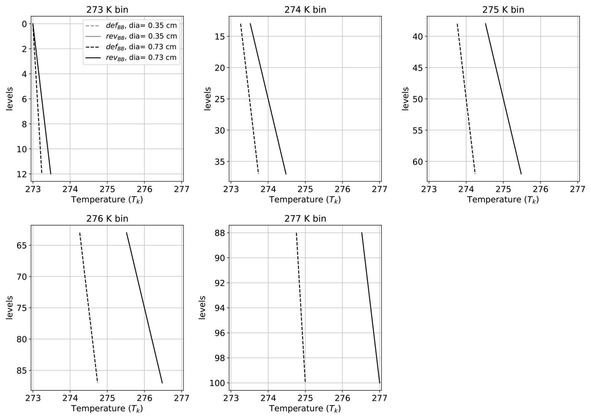
Figure A1 Profile of temperature (T_k) shown for 100 levels inside the melting layer using the def_BB and rev_BB schemes for two different diameters (shown by grey and black curves). These 100 levels are split across the five sub-layer temperature bins of the rev_BB scheme.

Figure A2 Same as Fig. A1 but for the melting fractions (f_m).

Figure A3 Same as above but for the backscattering coefficients.

The number of temperature levels N_levels used to discretize the melting layer is calculated following Eq. (A3):

$$\begin{array}{}\text{(A3)}& N_{\mathrm{levels}}={\displaystyle \frac{z_{\mathrm{layer}}}{\mathrm{d}z}}.\end{array}$$

It should be noted that the total number of levels N_levels is the same (100 here) in both schemes as the values of z_layer and dz are the same. These N_levels levels are split across the five temperature bins (i.e. five sub-melting layers) of the rev_BB scheme. This subdivision across the N_levels levels is intended to provide a smooth representation of the melting process. In both schemes, the scattering coefficients are divided by the same average width z_layer in Eqs. (A1) and (A2), regardless of the actual width of the selected temperature bin (1 K in the rev_BB scheme and 3 K in the def_BB scheme). Therefore, as the actual width of the sub-melting layers of the rev_BB scheme are smaller than in the def_BB scheme, this division results in an artificial reduction of the scattering coefficients in the rev_BB scheme as compared with the def_BB scheme. This feature was originally introduced unintentionally, but because it resulted in good fits to observations it was retained as a result. Were this feature to have been corrected, the results would have been much worse.

To understand the differences in physical processes between the def_BB and the rev_BB schemes, the variables of interest (i.e. temperature T_k, melted fraction f_m, and backscattering coefficient) are inter-compared.

In both schemes, the temperature profile T_k is calculated according to Eq. (A4):

$$\begin{array}{}\text{(A4)}& {\displaystyle }{T}_k{\displaystyle }=T_{\mathrm{fl}}+i_{\mathrm{level}}\cdot (T_{\mathrm{ml}}-T_{\mathrm{fl}})/N_{\mathrm{levels}},\end{array}$$

where i_level represents a given level within the melting layer depth. The temperature profiles are plotted for the five temperature bins (i.e. five sub-melting layers) of the revised scheme in Fig. A1 for two different diameters (0.35 cm in grey and 0.75 cm black plain curves) as a function of the height level i_level across the sub-melting-layer depth. For each of these levels, the temperature profile is also overlaid in dashed lines for these two selected diameters for the def_BB scheme. These profiles have been plotted at Ku band and for a hydrometeor content of $\mathrm{1}\times {\mathrm{10}}^{-\mathrm{4}}$ kg m³. Figure A1 shows that the temperature increases faster in the rev_BB scheme between two successive levels than in the def_BB scheme for a given temperature bin. Indeed, as the temperature at the bottom of the melting layer T_ml has been increased from 275 to 277 K in the rev_BB scheme, the slope of the temperature T_k profile is larger in the rev_BB scheme than in the def_BB scheme (see Eq. A4).

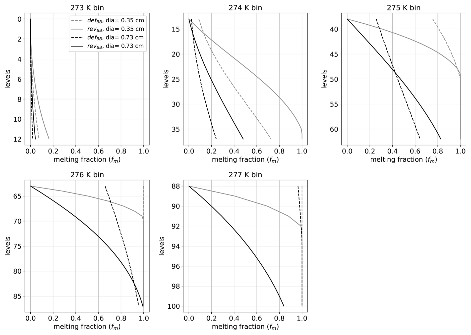
This difference in the temperature profiles directly impacts the fraction of melted particle f_m. A larger increase in the temperature values between two successive levels leads to a faster evaporation and, therefore, to a faster melting of the particle. This effect is depicted in Fig. A2, which shows the vertical profiles of melting fraction f_m across the melting-layer depth. It should be noted that f_m is always initialized at 0 for each of the five sub-melting layers in the rev_BB scheme, whereas it is continuous across the 100 levels for the def_BB scheme. However, despite this difference in their initialization, f_m is not necessarily smaller in rev_BB than in the def_BB scheme (see, for instance, the black curves for the 275 K bin). As it is starting from 0 instead of the value of the previous level in the original formulation, the fraction of melted particle f_m is usually smaller in the revised scheme for the first levels of the selected temperature bin, but then the fraction of melted particle f_m increases faster in the revised than in the default. For instance, for the 275 K temperature bin in Fig. A2, the dashed (def_BB scheme) and plain (rev_BB scheme) lines cross each other, even though f_m starts from 0 in the rev_BB scheme. The same behaviour also appears for the grey diameter at 274 K. This is due to the fact that the temperature increases faster between two successive levels in the rev_BB scheme.

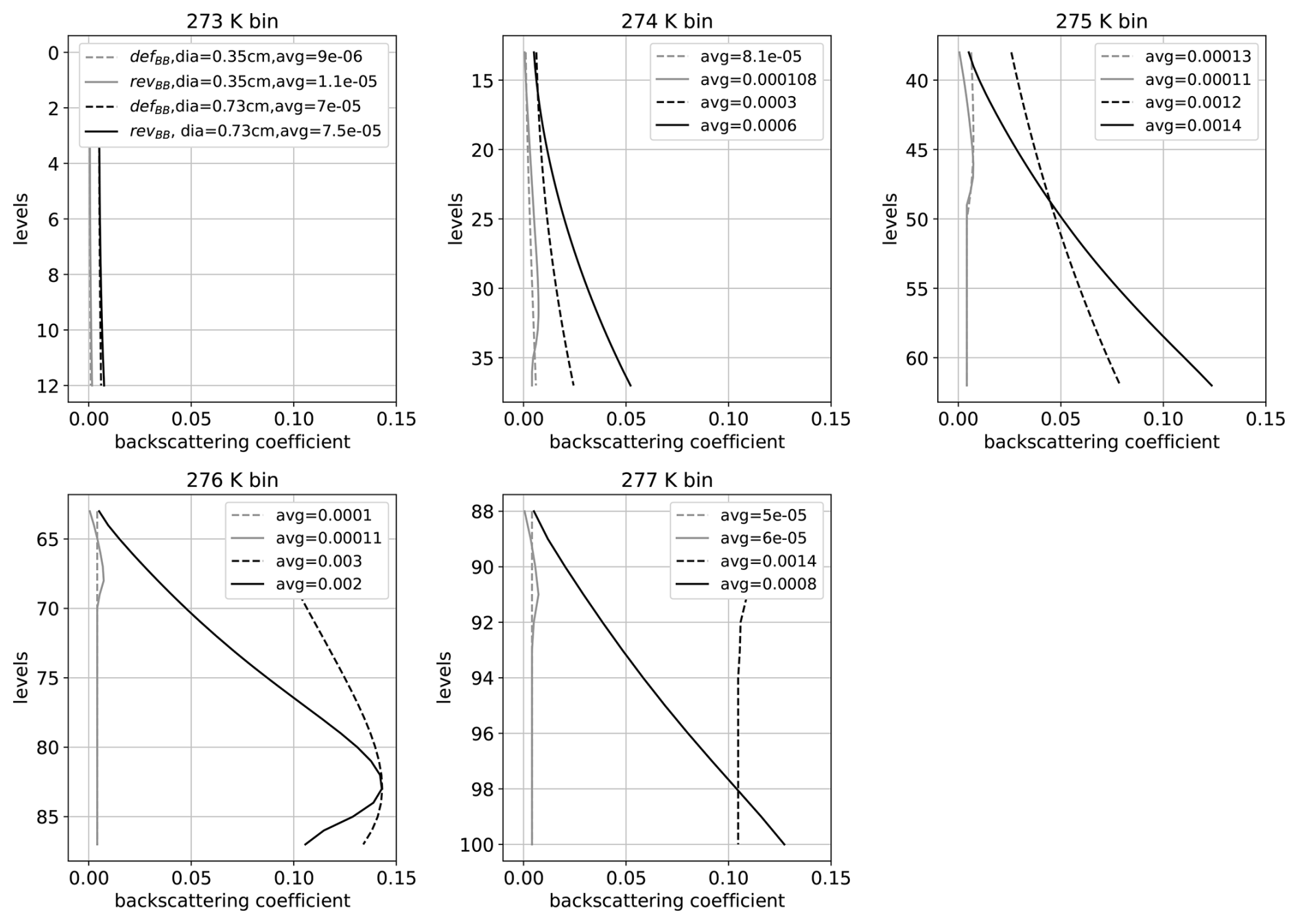
Similarly, the backscattering coefficient profiles are depicted in Fig. A3 for both schemes. Figure A3 shows that the backscattering coefficients are smaller at a given level of the rev_BB scheme only when their associated melted fraction (shown in Fig. A3) at this particular level are also smaller (see, for instance, the dashed and plain lines for the 275 K bin). As shown in Eq. (A2), the backscattering coefficients are then integrated over the number of levels of each temperature bin (i.e. sub-melting layer). These sub-layer averaged backscattering coefficients (divided by z_layer) are written in the legend of each panel in Fig. A3. These integrated coefficients depend on the evolution of the temperature and melted fraction profiles across this particular temperature bin. For instance, the revised scheme yields larger coefficients for the 274 and 275 K sub-melting layers as their associated fraction of melted particle is larger at most levels. However, for the 276 K bin, the backscattering coefficient is larger in the default scheme, but only because the differences in the initial values of f_m were too strong so that the revised scheme did not have time to reach the value of the default scheme. As there is only one bin in the default scheme (between 273 and 275 K), the backscattering coefficients of the def_BB scheme are averaged over the N_levels levels. The corresponding values are 0.00037 (diameter = 0.35 cm) and 0.0059 (diameter = 0.73 cm). These values are always larger than the sub-melting layer-averaged backscattering coefficients of the revised scheme. Consequently, the fact that the rev_BB scheme yields a more realistic bright band (as compared with the observations) is not only due to the division by the fixed average width z_layer, but also due to the fact that the integration has been split across five sub-melting layers.

Appendix B: Impact of the precipitation fraction on the simulated reflectivities

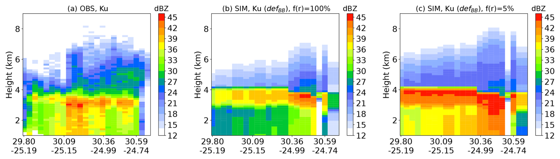
Figure B1 shows the vertical structure of observations (left panel) and RTTOV simulations (middle and right panels) with a convective hydrometeors fraction f_i(R) of 100 % (middle panel) and of 5 % (right panel) for the cloud which is depicted in Fig. 7. A convective hydrometeors fraction of 100 % (resp. 5 %) indicates that the predicted convective hydrometeor covers the full ARPEGE grid (resp. 5 % of the grid). As shown by Fig. B1, the simulated reflectivity is very sensitive to the convective precipitation fraction value. Fig. B1 demonstrates that small hydrometeor fraction f_i(R) significantly increases the reflectivity. The indirect relationship between f_i(R) and particle size distribution N(D) (see Eqs. 1 and 3) might cause this enhancement.

Figure B1 Vertical cross-section of (a) observation and (b, c) RTTOV simulations with convective precipitation fraction profiles of 100 % (b) and 5 % (c) for the same cloud as the one shown in Fig. 7.

Appendix C: Contingency table

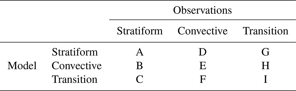
A contingency table is constructed as shown in Table C1. It is a matrix that measures the accuracy between observed and model-classified profiles. The diagonal elements A, E, and I represent the number of profiles which belong to the same class in both observations and the model. The non-diagonal elements are the misclassified profiles. For example, element B represents the number of profiles classified as stratiform in observations but convective by the simulations and similarly for others. The following categorical statistics are used:

1. Probability of detection (POD) is a measure of success of an algorithm that correctly classifies the profile into the stratiform or convective category.

2. False alarm ratio (FAR) determines the fraction of mismatched classified profiles between observation and model for a given classification category.

High POD and low FAR indicates higher accuracy. Equations (C1) and (C2) below illustrate the POD and FAR for stratiform events. Similarly, they are also computed for convective events. It is noted that transition profiles are used in the computation for POD and FAR, but the vertical structure is not discussed here because of the low occurrences mentioned in Table 2.

Table C1 Contingency table for the occurrence of stratiform, convective, and transition pixels.

$$\begin{array}{}\text{(C1)}& {\mathrm{POD}}_{\mathrm{stratiform}}={\displaystyle \frac{\mathrm{A}}{(\mathrm{A}+\mathrm{B}+\mathrm{C})}}\end{array}$$

$$\begin{array}{}\text{(C2)}& {\mathrm{FAR}}_{\mathrm{stratiform}}={\displaystyle \frac{\mathrm{D}+\mathrm{G}}{(\mathrm{A}+\mathrm{D}+\mathrm{G})}}\end{array}$$