Development and comparison of empirical models for all-sky downward longwave radiation estimation at the ocean surface using long-term observations

The ocean-surface downward longwave radiation (R_l) is one of the most fundamental components of the radiative energy balance, and it has a remarkable influence on air–sea interactions. Because of various shortcomings and limits, a lot of empirical models have been established for ocean-surface R_l estimation for practical applications. In this paper, based on comprehensive measurements collected from 65 moored buoys distributed across global seas from 1988 to 2019, a new model for estimating the all-sky ocean-surface R_l at both hourly and daily scales was built. The ocean-surface R_l was formulated as a nonlinear function of the screen-level air temperature, relative humidity, cloud fraction, total column cloud liquid, and ice water. A comprehensive evaluation of this new model relative to eight existing models was conducted under clear-sky and all-sky conditions at daytime/nighttime hourly and daily scales. The validation results showed that the accuracy of the newly constructed model is superior to that of other models, yielding overall root mean square error (RMSE) values of 13.44 and 8.34 W m⁻² under clear-sky conditions and 15.64 and 10.27 W m⁻² under all-sky conditions at hourly and daily scales, respectively. Our analysis indicates that the effects of the total column cloud liquid and ice water on the ocean-surface R_l also need to be considered in addition to cloud cover. Overall, the newly developed model has strong potential to be widely used.

1 Introduction

The downward longwave radiation (R_l) at the ocean surface is the thermal infrared (4–100 µm) radiative flux emitted by the entire atmospheric column over the ocean surface (Yu et al., 2018). The ocean-surface R_l is among the most important components of the heat flux across the ocean–atmosphere interface, which, in turn, shapes the climate state of both the atmosphere and the ocean (Caniaux et al., 2005; Trenberth et al., 2009; Fung et al., 1984). Therefore, an accurate estimate of the ocean-surface R_l is crucial for studies of air–sea interactions and climate and oceanic systems.

Although ocean-surface R_l is measured at most buoy sites, the available ocean-surface R_l measurements cannot meet the needs of various applications because of the small number of buoys currently employed (especially moored buoys) and their sparse distribution across global oceans. Another way to obtain the R_l at the ocean surface is by using satellite-based or model reanalysis products. The ocean-surface R_l from satellite-derived products, such as the International Satellite Cloud Climatology Project (ISCCP) (Rossow and Zhang, 1995; Young et al., 2018) and Clouds and the Earth's Radiant Energy System Synoptic Radiative Fluxes and Clouds (CERES/SYN1deg) (Doelling et al., 2013; Rutan et al., 2015), is usually generated using these satellite data and a radiative transfer model, which simulates the radiative transfer interactions of light absorption, scattering, and emission through the atmosphere with the input of given atmospheric parameters. However, radiative transfer models are not widely used in practice because of their complexity and the difficulties associated with collecting all essential inputs. The ocean-surface R_l provided in model reanalysis products, such as the fifth generation of the European Centre for Medium-Range Weather Forecasts atmospheric reanalysis of the global climate (ERA5) (Hersbach et al., 2020) and the Modern-Era Retrospective analysis for Research and Applications, version 2 (MERRA2) (Gelaro et al., 2017), is produced by assimilating various observations into an atmospheric model to get the optimal estimates of the state of the atmosphere and the surface (Gelaro et al., 2017). Previous studies have indicated that R_l estimates from satellite-based products are generally in better agreement with buoy measurements than those obtained from reanalysis products (Pinker et al., 2014, 2018; Thandlam and Rahaman, 2019). However, applications of the ocean-surface R_l from these two kinds of products are limited due to their coarse spatial resolutions (most of them are coarser than 1°), limited periods (especially satellite-based products), and discrepancies in accuracy and consistency (Cronin et al., 2019). Hence, many parameterization and empirical models for estimating ocean-surface R_l that can easily be implemented in practical use have been established during the past few decades (Bignami et al., 1995; Josey et al., 2003; Zapadka et al., 2001). Most of the commonly used R_l estimation models were established using the relationship between R_l and the relevant meteorological variables (i.e., air temperature, humidity, column-integrated water vapor (IWV), and cloud parameters) or oceanic parameters (i.e., bulk sea surface temperature), which are usually obtained from in situ measurements or model simulations (Li and Coimbra, 2019; Li et al., 2017; Berdahl, 2021). It is known that most R_l estimation models were originally developed for the land surface and were applied to the ocean surface directly without any alterations by assuming the atmospheric conditions are nearly the same over ocean and land surfaces (Bignami et al., 1995; Clark et al., 1974; Frouin et al., 1988; Josey et al., 2003). However, this assumption increases the uncertainty in R_l estimates because of the significantly different water vapor profiles over ocean and land surfaces (Bignami et al., 1995). A few models built specifically for R_l estimation at the ocean surface (Bignami et al., 1995; Josey et al., 2003; Zapadka et al., 2001) were typically developed using limited observations collected from buoy sites or cruise ships distributed within a specific region; hence, the robustness of these models was in doubt when applied globally. For example, Josey et al. (2003) proposed a model for R_l estimation in mid- to high-latitude seas with a satisfactory validation accuracy, but this new model performed worse over tropical seas, with a tendency to underestimate R_l by up to 10–15 W m⁻². Moreover, most of the existing R_l estimation models only work under clear-sky conditions, which are especially rare over ocean surfaces. Furthermore, most of these models only derive R_l at instantaneous scales, yet the R_l at the daily scale is preferred across a range of applications. Therefore, a new, easily implementable model that can derive accurate and robust R_l estimates at the global ocean surface under all-sky conditions at various temporal scales (e.g., instantaneous and daily) is required. More details about the existing R_l estimation models are given in Sect. 2.

In addition, according to Wang and Liang (2009b), the uncertainty in the ocean-surface R_l estimation should be less than 10 W m⁻² for climate diagnostic studies. However, the performances of the most commonly used R_l estimation models at the global ocean surface were not thoroughly evaluated in previous studies because of the few available in situ measurements. Fortunately, being aware of the significance of the energy budget in air–sea interactions (Centurioni et al., 2019), more and more platforms for radiative measuring have been built across global ocean surfaces during the past few decades, so relatively comprehensive ocean-surface R_l measurements can be collected today, which provide a good opportunity for modeling and comprehensive evaluations.

Overall, the main goal of this research is to establish a new empirical model for calculating the all-sky ocean-surface R_l at instantaneous and daily scales based on globally distributed moored buoy measurements and other ancillary information. A comprehensive evaluation is conducted on the newly developed model relative to eight commonly used models for ocean-surface R_l estimation under clear- and all-sky conditions at hourly and daily scales. The organization of this paper is as follows. A review of the eight commonly used R_l estimation models is presented in Sect. 2. Section 3 introduces the data sets used in this research and the methods, including the new model development and model evaluation. Section 4 shows the results of the model validation, comparison, and analysis. The key conclusions and discussions are provided in Sect. 5.

2 Review of previous models

Many models have been proposed for R_l calculation under various sky conditions at different temporal scales in previous studies. In this study, eight widely used models were selected for evaluation, and Table 1 shows their basic information. According to the sky conditions under which these models can be used, the eight R_l estimation models were divided into two classes: R_l models under clear-sky conditions and under all-sky conditions. Details of the eight models are provided one by one in the following section. Note that the downward direction is defined as positive in this study.

Table 1 Eight existing models for ocean-surface R_l estimation, with variables explained in Table 2.

2.1 Under clear-sky condition

Among the eight models, there are five R_l estimation models that can only be used under clear-sky conditions.

Brunt (1932) developed the first R_l estimation model (named Mod1) for land surfaces, which relates the monthly mean R_l to the screen-level water vapor and air temperature, as shown by Eq. (1):

$$\begin{array}{}\text{(1)}& R_{\mathrm{l}}=a_{\mathrm{1}}\mathit{\sigma }{T}_{\mathrm{a}}^{\mathrm{4}}\left(\mathrm{1}+b_{\mathrm{1}}\sqrt{e}\right),\end{array}$$

where a₁ and b₁ are empirical coefficients; T_a is the monthly mean screen-level air temperature (K); e is the monthly mean screen-level water vapor pressure (mbar); and σ is the Stefan–Boltzmann constant, defined as $\mathrm{5.67}\times {\mathrm{10}}^{-\mathrm{8}}$ W (m² K⁴)⁻¹. In the study of Brunt (1932), the two coefficients a₁ and b₁ were suggested as 0.52 and 0.125 based on observations collected from Benson, South Oxfordshire, England. The validation results of Mod1 showed a correlation coefficient as high as 0.97 based on the collected samples. However, Swinbank (1963) pointed out that the validation results of Mod1 for other regions, where variations in the humidity and T_a were different from those in Benson, were worse. Despite these limitations, as the first empirical R_l estimation model in a simple format, Mod1 has been widely used to construct the coupling between hydrological and atmospheric models (Habets et al., 1999; Lohmann et al., 1998).

Different from Mod1, the model developed by Idso and Jackson (1969) (named Mod2) was based on the theoretical consideration that the effective emittance of an atmosphere is solely temperature dependent; hence, the screen-level T_a is the only input of Mod2 for calculating R_l:

$$\begin{array}{}\text{(2)}& R_{\mathrm{l}}=\mathit{\sigma }{T}_{\mathrm{a}}^{\mathrm{4}}\left\{\mathrm{1}-a_{\mathrm{2}}\exp \left(-b_{\mathrm{2}}{\left(\mathrm{273}-T_{\mathrm{a}}\right)}^{\mathrm{2}}\right)\right\},\end{array}$$

where a₂ and b₂ are empirical coefficients, which were defined as 0.261 and 7.770 $\times {\mathrm{10}}^{-\mathrm{4}}$, respectively, by Idso and Jackson (1969) based on experimental data at four sites located in Arizona, Alaska, Australia, and the Indian Ocean, obtained at intervals of 5 to 15 min. Idso and Jackson (1969) thought that Mod2 might be efficient at all latitudes in different seasons, as it has been developed by using observations from diverse locations. Since its publication, Mod2 has been employed in relevant research, like evaporation estimation (Cleugh et al., 2007; Vertessy et al., 1993) and ocean-ice modeling (Saucier et al., 2003).

Afterwards, Brutsaert (1975) proposed a simple model for computing R_l by directly solving Schwarzschild's transfer equation (Schwarzschild, 1914) under clear skies and standard atmospheric conditions (i.e., the US 1962 standard atmosphere). This model is denoted as Mod3 and is described as follows:

$$\begin{array}{}\text{(3)}& R_{\mathrm{l}}=a_{\mathrm{3}}\mathit{\sigma }{T}_{\mathrm{a}}^{\mathrm{4}}{\left(e/T_{\mathrm{a}}\right)}^{\mathrm{1}/\mathrm{7}},\end{array}$$

where a₃ is defined as a constant equal to 1.24, as determined during Schwarzschild's transfer equation solving process. Explicit physical theory is reflected in Mod3. The term $(e/T_{\mathrm{a}}{)}^{\mathrm{1}/\mathrm{7}}$, regarded as the atmospheric emissivity, tends to zero when the water vapor content is very little. However, Prata (1996) indicated that the atmospheric emissivity tends to a certain constant value even without water vapor, such as values from 0.17 to 0.19 when only CO₂ is present (Staley and Jurica, 1972). The estimates from Mod3 are usually used as the necessary inputs of hydrological models (Pauwels et al., 2007; Rigon et al., 2006) and climate models (Mills, 1997).

Aase and Idso (1978) found that Mod2 and Mod3 performed poorly when T_a was below freezing. To address this issue, Satterlund (1979) proposed a model (named Mod4) to compute R_l by reformatting T_a and e as follows:

$$\begin{array}{}\text{(4)}& R_{\mathrm{l}}=a_{\mathrm{4}}\mathit{\sigma }{T}_{\mathrm{a}}^{\mathrm{4}}\left[\mathrm{1}-\exp \left(-e^{T_{\mathrm{a}}/\mathrm{2016}}\right)\right],\end{array}$$

where a₄ is an empirical coefficient defined as 1.08 by Satterlund (1979) and is based on collected daily R_l measurements at one site in Sidney, Montana, USA. After validation and comparison, Satterlund (1979) concluded that Mod4 outperformed Mod2 and Mod3 under extreme conditions in terms of temperature and humidity and performed comparably with the two models in other cases. As such, the R_l estimates from Mod4 have been used in studies on snowpack evolution (Douville et al., 1995) and hydrological models (Schlosser et al., 1997). However, because the model does not contain a constant term, the application of Mod4 should be done with caution if the surface water vapor pressure is very close to zero.

With the development of radiation-measuring instruments and technology, several new R_l estimation models have been proposed, such as the following model proposed by Prata (1996) (named Mod5):

$$\begin{array}{}\text{(5)}& \begin{array}{rl}{R}_{\mathrm{l}}=\mathit{\sigma }{T}_{\mathrm{a}}^{\mathrm{4}}[& \mathrm{1}-\left(\mathrm{1}+\mathrm{46.5}\left({\displaystyle \frac{e}{T_{\mathrm{a}}}}\right)\right)\\ & \exp \left\{-{\left(a_{\mathrm{5}}+\mathrm{46.5}{b}_{\mathrm{5}}\left({\displaystyle \frac{e}{T_{\mathrm{a}}}}\right)\right)}^{\mathrm{1}/\mathrm{2}}\right\}],\end{array}\end{array}$$

where a₅ and b₅ are empirical coefficients, defined as 1.2 and 3.0 in the study of Prata (1996) and Robinson (1947, 1950). As with Mod1–Mod4, Mod5 is also dependent on T_a and e but contains a majorly revised right term (in the square brackets), which is regarded as the emissivity. After extensive validation and comparison, Prata (1996) claimed Mod5 outperformed or performed similarly to other R_l estimation models, including Mod1–Mod4, in areas within the polar region, mid-latitudes, and tropical regions. Hence, Mod5 has been widely applied, from snowmelt modeling studies (Jost et al., 2009) to urban energy budget studies (Nice et al., 2018; Oleson et al., 2008).

To sum up, all five R_l estimation models (Mod1–Mod5) that only work under clear-sky conditions take T_a and/or e as inputs. Such an approach is in agreement with the research of Kjaersgaard et al. (2007), who found that R_l is mainly emanated from the low-level atmosphere that can be adequately characterized in terms of T_a and humidity under clear-sky conditions (Diak et al., 2000; Ellingson, 1995; Prata, 1996). Moreover, the five models were all established by using measurements from different regions at various timescales, and they can be employed at any timescale (see Table 1) regardless of the temporal resolution of the original measurements used for modeling.

2.2 Under all-sky condition

Three R_l estimation models that can work under all-sky conditions were evaluated in this paper. Compared to the above five models, ancillary information (e.g., clouds) should be taken into account in addition to T_a and e in the three models, and the three models were developed specifically for ocean surfaces.

Based on the model developed by Clark et al. (1974) for the all-sky net longwave radiation for the ocean-surface (R_lnet, the difference between the downward and upward longwave radiation) calculation, Josey et al. (2003) proposed a revised model (named Mod6) to estimate the all-sky ocean-surface R_l by getting rid of the ocean-surface upward longwave radiation as

$$\begin{array}{}\text{(6)}& \begin{array}{rl}& R_{\mathrm{l}}=\\ & {\displaystyle \frac{{\mathit{\epsilon }}_{\mathrm{s}}\mathit{\sigma }{\text{SST}}^{\mathrm{4}}-{\mathit{\epsilon }}_{\mathrm{s}}\mathit{\sigma }SS{T}^{\mathrm{4}}\left(a_{\mathrm{6}}+b_{\mathrm{6}}\sqrt{e}\right)\left(\mathrm{1}-\mathit{\lambda }{C}^{\mathrm{2}}\right)-\mathrm{4}{\mathit{\epsilon }}_{\mathrm{s}}\mathit{\sigma }{\text{SST}}^{\mathrm{3}}\left(\text{SST}-T_{\mathrm{a}}\right)}{\mathrm{1}-{\mathit{\alpha }}_{\mathrm{s}}}},\end{array}\end{array}$$

where ε_s is the sea surface emissivity, defined as a constant value of 0.98, and SST is the sea surface temperature (K); hence, the term ε_sσSST⁴ is the upward longwave radiation at the ocean surface. Here, α_s is the sea surface longwave radiation reflectivity, defined as a constant value of 0.045; C is the cloud cover (0–1; dimensionless); λ is a latitude-dependent coefficient that represents the cloud amount; and a₆ and b₆ are empirical coefficients. Based on measurements (i.e., R_l, T_s, and C) collected from the Chemical and Hydrographic Atlantic Ocean Section (CHAOS) in the northeast Atlantic in 1998, a₆ and b₆ were determined as 0.39 and −0.05 (Clark et al., 1974; Josey et al., 2003), and λ at a given latitude can be taken from Josey et al. (1997). Josey et al. (2003) validated Mod6, and the results showed that Mod6 tended to overestimate the instantaneous R_l measurements from CHAOS by 11.70 W m⁻². The estimates from Mod6 have been applied in hydrodynamic models (Grayek et al., 2011) and atmospheric boundary layer models (Deremble et al., 2013).

Based on hourly cruise measurements (i.e., R_l, T_a, and C) collected in the Mediterranean Sea during the period from 1989 to 1992, Bignami et al. (1995) proposed an empirical model to calculate the ocean-surface all-sky R_l (named Mod7) as follows:

$$\begin{array}{}\text{(7)}& R_{\mathrm{l}}=\mathit{\sigma }{T}_{\mathrm{a}}^{\mathrm{4}}\left(a_{\mathrm{7}}+b_{\mathrm{7}}e\right)\left(\mathrm{1}+c_{\mathrm{7}}{C}^{\mathrm{2}}\right),\end{array}$$

where a₇, b₇, and c₇ are empirical coefficients defined as 0.684, 0.0056, and 0.1762, respectively. Bignami et al. (1995) presented validated root mean square error (RMSE) values for Mod7, which ranged from ∼ 14 W m⁻² at the hourly scale to ∼ 9 W m⁻² at the daily scale. Mod7 has been utilized by the Mediterranean Forecasting System in predictions of currents and biochemical parameters (Pinardi et al., 2003), coupled ocean–atmosphere climate models (Dubois et al., 2012), and the generation of the Atlantic Ocean heat flux climatology (Lindau, 2012).

Also based on the measurements collected from CHAOS, Josey et al. (2003) assessed the accuracy of Mod7 and found that this model tended to underestimate the all-sky R_l by 12.10 W m⁻² at the instantaneous scale. After analyzing the shortcomings of Mod6 and Mod7, Josey et al. (2003) proposed a new model (named Mod8) for all-sky ocean-surface R_l calculation through a revision of T_a by using the same samples:

$$\begin{array}{}\text{(8)}& R_{\mathrm{l}}=\mathit{\sigma }{\left\{T_{\mathrm{a}}+a_{\mathrm{8}}{C}^{\mathrm{2}}+b_{\mathrm{8}}C-c_{\mathrm{8}}+d_{\mathrm{1}}\left(D+e_{\mathrm{1}}\right)\right\}}^{\mathrm{4}},\end{array}$$

where a₈, b₈, c₈, d₁, and e₁ are empirical coefficients determined as 10.77, 2.34, 18.44, 0.84, and 4.01, respectively; D is the dew point depression; and T_a is the temperature (K) (see Eq. 11). Estimates of R_l obtained with Mod8 agreed within 2 W m⁻² with respect to the mean bias of 10 min measurements at middle to high latitudes. The estimates from Mod8 have been used as essential input in simulations of ocean–atmosphere interactions in an Arctic shelf (Cottier et al., 2007).

Overall, it was thought that variations in the all-sky ocean-surface R_l were related to T_a, e, and cloud information (e.g., cloud cover and cloud amount) in previous studies. However, Fung et al. (1984) pointed out that other relevant cloud information, such as the cloud base height (CBH) and cloud optical thickness, also has a significant influence on ocean-surface longwave radiation. Therefore, more efforts should be made to increase the R_l estimation accuracy under all-sky conditions.

3 Data and methodology

In order to develop a new all-sky ocean-surface R_l estimation model, the meteorological and radiative observations from 65 moored buoys and the cloud parameters from the ERA5 reanalysis product from 1988 to 2019 were applied. Afterwards, the newly developed model and the eight commonly used models (Mod1–Mod8) were evaluated against the moored R_l measurements under clear- and all-sky conditions at hourly and daily scales.

3.1 Data and pre-processing

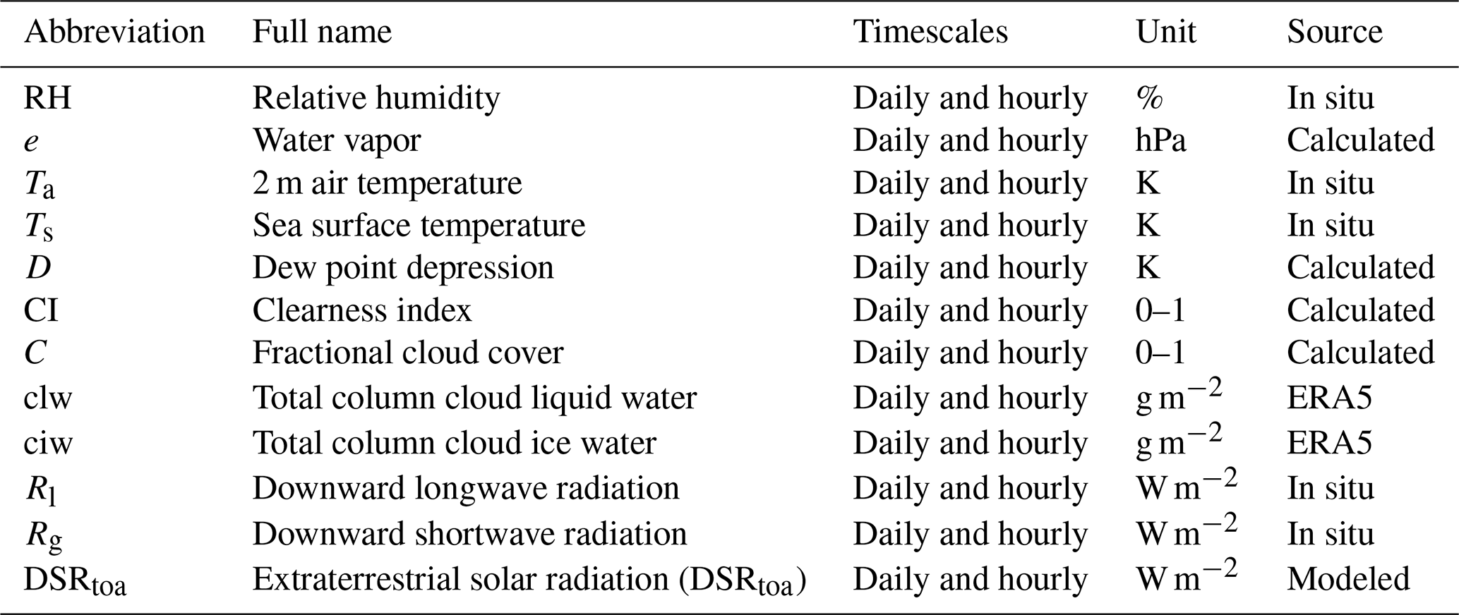
Table 2 lists all the variables employed in this paper and their information. The instantaneous timescale can be defined as timescales ranging from a 3 min average to an hourly average (Bignami et al., 1995; Wang and Liang, 2009a); hence, two timescales, hourly and daily, were considered in this study for model evaluation, as in previous studies (Bilbao and de Miguel, 2007; Kjaersgaard et al., 2007; Sridhar and Elliott, 2002). Note that Mod1 was also used at the two timescales (Guo et al., 2019), though it was originally established with monthly samples. More details about the data are given below.

Table 2 Variables: explanations and sources.

3.1.1 Measurements from moored buoys

All measurements were collected from 65 moored buoy sites, whose latitudes range from 47° S to 59.5° N, as shown in Fig. 1. The majority of moored buoy sites were located in tropical seas (23.5° S–23.5° N), and relatively few buoys were in the high-latitude seas of the Northern Hemisphere (> 50° N) and the mid- to high-latitude seas of the Southern Hemisphere (> 30° S).

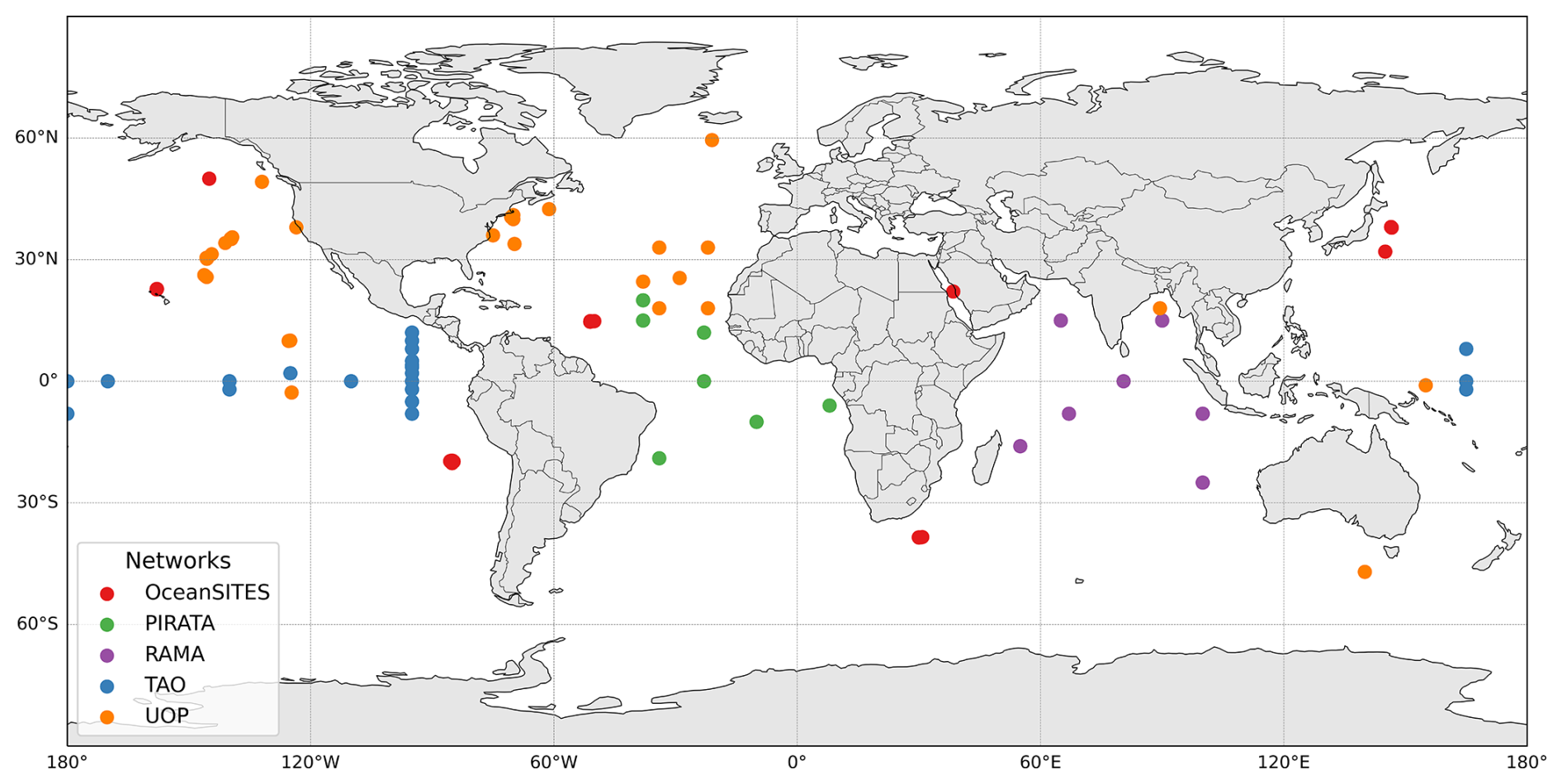
Figure 1 Spatial distribution of the 65 moored buoys.

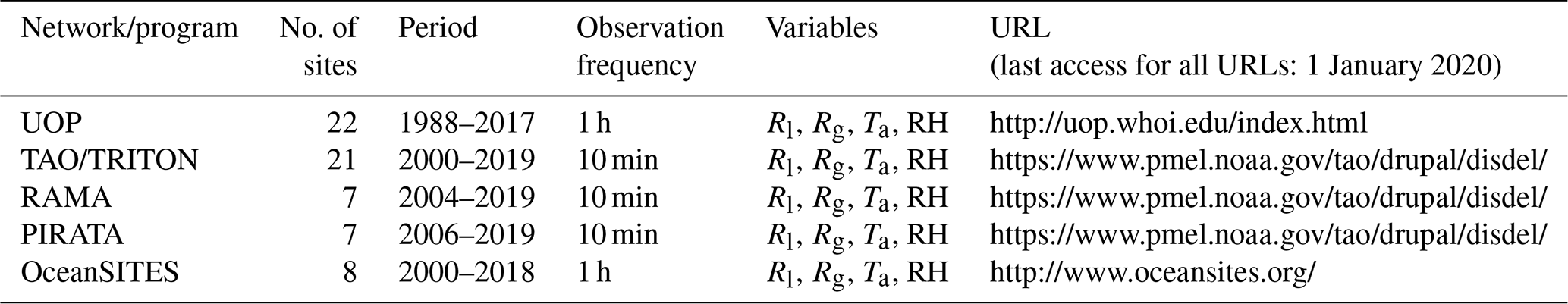
The moored buoy sites in this study belong to five well-known observation networks/programs, including the Upper Ocean Processes Group (UOP), the Tropical Atmosphere Ocean/Triangle Trans-Ocean Buoy Network (TAO/TRITON), the Pilot Research Moored Array in the Tropical Atlantic (PIRATA), the Research Moored Array for African–Asian–Australian Monsoon Analysis and Prediction (RAMA), and OceanSITES. Launched by the Woods Hole Oceanographic Institution (WHOI), UOP mainly focuses on studying the physical processes of the air–sea interface and the epipelagic, and its buoys are equipped with oceanographic and meteorological sensors. The UOP measurements accurately quantify annual cycles of wind stress and net air–sea heat exchange in the Southern Ocean (Schulz et al., 2012). A total of 22 sites form the UOP, and data from all sites were used in this study. TAO/TRITON (McPhaden et al., 1998) in the tropical Pacific, PIRATA (Bourlès et al., 2008) in the tropical Atlantic, and RAMA in the tropical Indian Ocean (McPhaden et al., 2009) are all part of the Global Tropical Moored Buoy Array (GTMBA) program (McPhaden et al., 2010). Extensive quality control was done by GTMBA prior to dissemination of the data (Freitag et al., 1999, 2001; Lake et al., 2003; Medovaya et al., 2002), and they have been used for monitoring, understanding, and forecasting the El Niño–Southern Oscillation (ENSO) and monsoon variability (McPhaden et al., 2009). Data from 35 GTMBA sites (TAO, 21; PIRATA, 7; RAMA, 7) were used in this study. The OceanSITES network is composed of buoys funded by oceanographic researchers across the globe. The goal of the OceanSITES program is to facilitate the use of high-quality multidisciplinary data from fixed sites in the open ocean (Cronin et al., 2019). Eight sites from OceanSITES were utilized, specifically OS_PAPA, OS_KAUST, OS_NTAS, OS_KEO, OS_ARC, OS_JKEO, OS_STRATUS, and OS_WHOTS. In this study, the routine measurements made at moored buoys, including radiative measurements (e.g., ocean-surface downward shortwave radiation R_g) and meteorological measurements (e.g., T_a and RH), were collected and used; other variables (e.g., e, D, and CI) were calculated from these measurements. More information regarding these data sets can be found in Table 3.

Table 3 Descriptions of different networks.

Radiative measurements

At each moored buoy, R_l is routinely measured by an Eppley precision infrared radiometer (PIR) with a nominal accuracy of ±1 % (Payne and Anderson, 1999), and R_g is routinely measured by an Eppley Laboratory precision spectral pyranometer (PSP) with a calibration accuracy of ±2 % (Freitag et al., 1994). The PIR and PSP are deployed approximately 3 m above sea level. All measurements are quality controlled by their providers. To ensure data quality, a two-step approach was implemented: (1) only observations flagged as “high quality” by the data providers were considered, and (2) data were manually inspected by the authors for any irregularities. Additionally, R_l measurements above 450 W m⁻² were removed, as suggested by Josey et al. (2003).

As pointed out by Pascal and Josey (2000), the main errors in measuring R_l are from the shortwave leakage and differential heating of the sensor. These errors (ΔR_l) in R_l observations can be corrected according to Pascal and Josey (2000). However, this correction was not applied in our study, as (a) differential heating corrections had already been performed by the data providers, and (b) the R_l spikes associated with sensor degradation were not present across all deployments, making a universal correction inappropriate. We also compared the results with and without the correction and found that the conclusions remained unchanged.

All R_l measurements whose sampling frequency was less than 1 h were aggregated into hourly means as long as 80 % of the measurements in 1 h were available, and the hourly data were aggregated into daily means as long as 24-hourly data in 1 d were available.

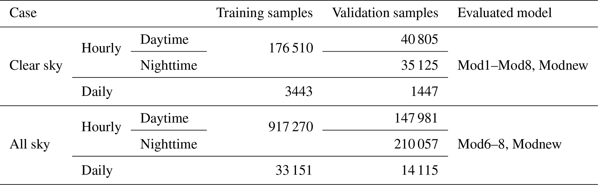
Note that the errors in the measured R_g induced by buoy rocking motions, sensor tilting, and aerosol accumulation (Medovaya et al., 2002) were too small to be considered here. In total, 47 266 samples at the daily scale and 1 275 308 samples at the hourly scale during the period from 1988 to 2019 were used in this study. For better comparison, the hourly samples used for independent validation were further divided into daytime (R_g > 120 W m⁻²) and nighttime conditions (R_g ≤ 120 W m⁻²), with 147 981 samples in daytime and 210 057 in nighttime.

Meteorological and oceanic variables

Two meteorological measurements, RH and T_a, were collected at the moored buoy sites. The instrument used for measuring RH and T_a is a Rotronic MP-100F, deployed about 3 m above sea level. The instrument produced accuracies of 2.7 % and 0.2 K (Lake et al., 2003) for RH and T_a, respectively, which are also too small to influence the accuracy of the R_l estimation. Similar to the radiative measurements, RH and T_a were both strictly screened and then aggregated into hourly and daily means.

On the other hand, the sea surface temperature (SST) was measured at about 1 m below sea level using a high-accuracy conductivity and temperature recorder (SBE37/39; Sea Bird Electronics) with an accuracy of 0.002 K. According to Donlon et al. (2002), there is a strong correlation between body SST and skin SST. Although wind speed has a significant effect on this relationship, a constant correction offset can be applied when the wind speed exceeds 6 m s⁻¹ (Alappattu et al., 2017). In fact, 83 % of the samples had wind speeds above 4 m s⁻¹, and, as suggested by Vanhellemont (2020), the bulk SST measured at moored buoys can be adjusted to the skin SST by using a correction offset of 0.17 K.

Calculation of other variables

Three variables, including e, D, and CI, were calculated separately with the RH, T_a, and R_g measurements. Therefore, these three variables at hourly and daily scales were obtained from the corresponding measurements. Specifically, the daily (hourly) mean e was calculated from the daily (hourly) RH using the following equation:

$$\begin{array}{}\text{(9)}& e=\mathrm{6.1121}{\displaystyle \frac{\text{RH}}{\mathrm{100}}}\exp \left({\displaystyle \frac{\mathrm{17.502}{T}_{\mathrm{a}}}{T_{\mathrm{a}}+\mathrm{240.97}}}\right).\end{array}$$

The daily (hourly) dew point depression D was calculated according to Josey et al. (2003) and Henderson-Sellers (1984) as

$$\begin{array}{}\text{(10)}& D=\mathrm{34.07}+\mathrm{4157}/\ln \left(\mathrm{2.1718}\times {\mathrm{10}}^{\mathrm{8}}/e\right)-T_{\mathrm{a}}.\end{array}$$

Note that Eq. (10) only works when T_a is in the range of −30 to 50 °C (Buck, 1981), and T_a should be in degrees Celsius. The clearness index (CI) is calculated as the ratio of the surface R_g to the extraterrestrial solar radiation (DSR_toa) (Ogunjobi and Kim, 2004). CI generally represents the atmospheric transmissivity affected by permanent gases, aerosols, and the optical thickness of the clouds (Alados et al., 2012; Flerchinger et al., 2009; Gubler et al., 2012; Jiang et al., 2015; Meyers and Dale, 1983), and it is widely used in radiation-related research (Iziomon et al., 2003; Jiang et al., 2015, 2016; Payne, 1972). The value of CI is between 0 and 1, where a larger CI value represents a clearer sky. The hourly CI can be calculated as follows:

$$\begin{array}{}\text{(11)}& \text{CI}={\displaystyle \frac{R_{\mathrm{g}}}{{\text{DSR}}_{\mathrm{toa}}}}.\end{array}$$

However, during nighttime, the hourly CI cannot be calculated using Eq. (11) directly because of a lack of R_g values; hence, it was calculated based on a 24 h solar radiation window centered on the hourly observations, as suggested by Flerchinger et al. (2009). The daily CI was calculated as the average of all hourly CI values in a day for the sake of considering atmospheric variations during nighttime.

In this paper, CI was utilized to determine the condition as clear sky when its value was greater than 0.7 at both hourly and daily scales. Additionally, it was found that the cloud cover derived from CI would help to improve the model performance after multiple experiments, especially during nighttime. Therefore, CI was also used to calculate the cloud cover. Specifically, the cloud fraction was linearly interpolated between C = 1.0 at a CI value of 0.4 for complete cloud cover and C = 0.0 at a CI value of 0.7 for cloudless conditions, both at daily and hourly scales, according to Flerchinger et al. (2009). Because of the different calculation of CI during daytime and nighttime, the uncertainty in the calculated cloud cover was different; hence, the R_l estimates at the hourly scale were further examined during daytime and nighttime. Therefore, all meteorological factors (RH, T_a, e, and D) at daily and hourly scales were prepared accordingly.

3.1.2 Cloud parameters from the ERA5 reanalysis data set

As described above, the cloud cover represented by the cloud fraction (C) is usually taken into account when estimating R_l affected by clouds. However, in this study, two more cloud-related parameters, including clw and ciw (see Table 2), from the ERA5 reanalysis product were also considered in the modeling. The total amount of liquid water per unit area in the air column from the base to the top of the cloud is called the total column cloud liquid water (clw), and its chilled counterpart (ice) is called the total column cloud ice water (ciw) (Nandan et al., 2022). ERA5 is the fifth-generation atmospheric reanalysis product, and it was produced based on 4D-Var data assimilation using the Integrated Forecasting System (IFS) with an enhanced spatial resolution (0.25°) and time resolution (hourly) compared to its previous version ERA-Interim (Hoffmann et al., 2019) from 1979 to present. Clouds in ERA5 are represented by a fully prognostic cloud scheme, in which cloud fractions and cloud condensates obey mass balance equations (Tiedtke, 1993). The ERA5 clw values are in good agreement with those obtained from radiosonde observations (Nandan et al., 2022). Overall, relative to ERA-Interim, ERA5 shows reduced biases in the total ice water path versus other satellite-based observational products. Therefore, the two cloud parameters were extracted from the locations of the 65 moored buoy sites directly at the hourly scale, and then their daily means were calculated by averaging the 24 valid hourly values. The ERA5 cloud product is available on the Climate Data Store (CDS) cloud server (https://www.ecmwf.int/en/forecasts/dataset/ecmwf-reanalysis-v5, last access: 28 June 2025).

Overall, 70 % of the samples at each moored buoy site, including 33 151 daily samples and 917 270 hourly samples, were randomly selected for new model training and calibration of the eight previous models (Mod1–Mod8). The other 30 % of the data at each site, including 14 115 daily samples and 358 038 hourly samples (daytime: 147 981; nighttime: 210 057), were used for model validation.

3.2 Methodology

A new model that can estimate ocean-surface R_l under all-sky conditions at both hourly and daily scales was developed based on the moored measurements and ERA5 cloud parameters. Moreover, the eight evaluated R_l models were all recalibrated so as to evaluate the model's accuracy objectively. Based on the corresponding validation samples, the R_l values produced by the nine models were compared under clear-sky and all-sky conditions at hourly and daily scales, where the comparison at the hourly scale was further divided into daytime and nighttime values.

3.2.1 New R_l estimation model development

As mentioned above, T_a and the humidity-related factors (e.g., RH) were enough to characterize the variations in R_l under clear-sky conditions. However, for cloudy skies, R_l is enhanced by emission from the cloud base (Wang et al., 2020; Yang and Cheng, 2020). Cloud cover is one of the most commonly used cloud-related parameters. In addition, theoretically, the cloudy-sky R_l is significantly influenced by the cloud's base temperature, which is determined by the CBH; hence, the CBH is thought to be necessary in determining R_l under cloudy-sky conditions (Viúdez-Mora et al., 2015). However, it is difficult to obtain the CBH accurately, especially for partly cloudy skies (Zhou and Cess, 2001) because of the unavailability of the cloud's geometrical thickness (Yang and Cheng, 2020). Therefore, other parameters that can provide information on the CBH were explored. In the study of Hack (1998), a physical correlation between clw and CBH was revealed in most cases, while clw was successfully used as an effective surrogate of the CBH in the study of Zhou and Cess (2001). However, Zhou et al. (2007) pointed out that the effects of ice clouds on R_l should also be considered when the atmospheric water vapor is low or at high latitudes, which means that ciw also needs to be taken into account. Inspired by these studies, clw and ciw, both in logarithmic form, were introduced in the development of a new model named Modnew, in which R_l under all-sky conditions at the ocean surface was related to five parameters, including T_a, RH, clw, ciw, and C. Modnew was trained by the corresponding training samples at hourly and daily scales. Details of the development of the new model presented in the present study are given in Sect. 4.1.

3.2.2 Model performance evaluation

Table 4 lists the different cases for the R_l model comparison. As shown in Table 4, the nine evaluated models (Mod1–Mod8 and Modnew) were all used for clear-sky R_l estimation at both hourly and daily scales, while only four models (Mod6–Mod8 and Modnew) were evaluated under all-sky conditions. Three metrics were employed to present the model accuracy: R², the RMSE, and bias. Generally, all three statistics were calculated to evaluate the accuracy of the different models, but the RMSE values had larger weights.

Table 4 Detailed information of the six cases considered in the model evaluation.

4 Results and analysis

In this section, Modnew is introduced first, and then the validation results of the nine evaluated models under various conditions are compared and analyzed. Lastly, further analyses are conducted on Modnew.

4.1 Modnew development

As mentioned above, the ocean-surface R_l in Modnew is related to five parameters (T_a, clw, RH, C, and ciw) for hourly and daily scales under all-sky conditions. To better understand the contribution made by each variable to R_l, the five parameters were introduced into Modnew gradually. Taking the daily all-sky R_l as an example, it was first characterized only by the fourth power of T_a based on the Stefan–Boltzmann law as follows:

$$\begin{array}{}\text{(12)}& R_{\mathrm{l}}=a_{\mathrm{new}}\mathit{\sigma }{T}_{\mathrm{a}}^{\mathrm{4}}+b_{\mathrm{new}},\end{array}$$

where a_new and b_new are empirical coefficients, determined as 0.85 and 14.96, respectively, based on the daily training samples. Then, the correlations between the model residuals in R_l (referred to as ΔR_l), which define the difference between the in situ R_l measurements and the R_l estimates from Eq. (13) and the other four parameters (clw, RH, C, and ciw), were explored one by one. The results can be found in Fig. 2.

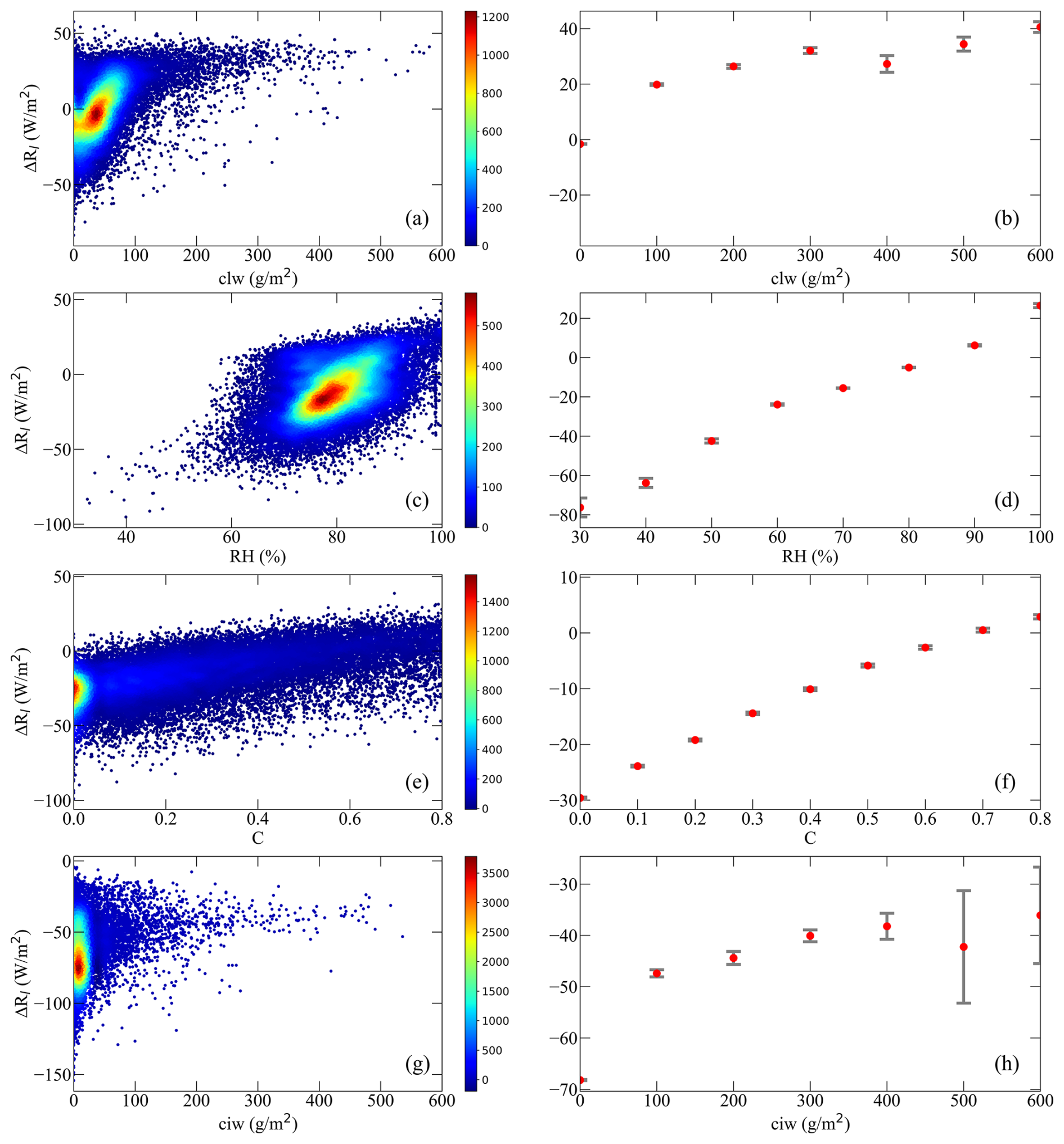
Figure 2 The scatter plots between the model residuals, ΔR_l, from Eq. (13) and (a) clw, (c) RH, (e) C, and (g) ciw. Panels (b), (d), (f), and (h) are their corresponding box plots. In the left column, the color bar represents points per unit area. In the right column, the dots indicate the mean value of ΔR_l (ME), while the vertical lines represent the standard error of the mean (SEM).

Figure 2a, c, e, and g present scatter plots between ΔR_l and clw, RH, C, and ciw, respectively. In order to show their relationships better, the corresponding box plots were created, in which the mean of ΔR_l and its standard error (SEM) for each bin of the four parameters (in 10 % increments) were calculated and presented in Fig. 2b, d, f, and h, respectively. Specifically, ΔR_l varied with clw and ciw in a logarithmic relationship (Fig. 2b and h, respectively), and with RH (Fig. 2d) and C (Fig. 2f) in approximately linear relationships. We found that by introducing C, RH, clw, and ciw into Eq. (13) gradually, the RMSE was reduced from 17.48 W m⁻² with Eq. (13) to 12.61, 10.92, 10.11, and 9.87 W m⁻², and the level of R² increased accordingly from 0.64 to 0.81, 0.86, 0.88, and 0.89, respectively. Hence, clw, RH, C, and ciw were introduced into Eq. (13) in their appropriate forms, and the final equation was taken as Modnew:

$$\begin{array}{}\text{(13)}& \begin{array}{rl}{R}_{\mathrm{l}}& =a_{\mathrm{new}}\mathit{\sigma }{T}_{\mathrm{a}}^{\mathrm{4}}+b_{\mathrm{new}}C+c_{\mathrm{new}}\ln (\mathrm{1}+\text{clw})\\ & +d_{\mathrm{new}}\ln (\mathrm{1}+\text{ciw})+e_{\mathrm{new}}\text{RH}+f_{\mathrm{new}},\end{array}\end{array}$$

where a_new, b_new, c_new, d_new, e_new, and f_new are empirical coefficients. In this study, these coefficients were determined as 1.06, 39.05, 4.91, −2.06, 0.91, and −177.53, respectively. Figure 3a shows that the overall training accuracy of the estimated all-sky ocean-surface R_l from Modnew was satisfactory, yielding an R² of 0.89, RMSE of 9.99 W m⁻², and nearly no bias. Afterwards, Eq. (14) was used to determine the hourly ocean-surface R_l based on the corresponding hourly training samples (see Table 4). The hourly results shown in Fig. 3b were satisfactory, with an R² of 0.78, RMSE of 15.72 W m⁻², and nearly no bias. Note that the R_l measurements whose values were larger than 450 W m⁻² were thought to be unreasonable and were manually removed (see Sect. 3.1).

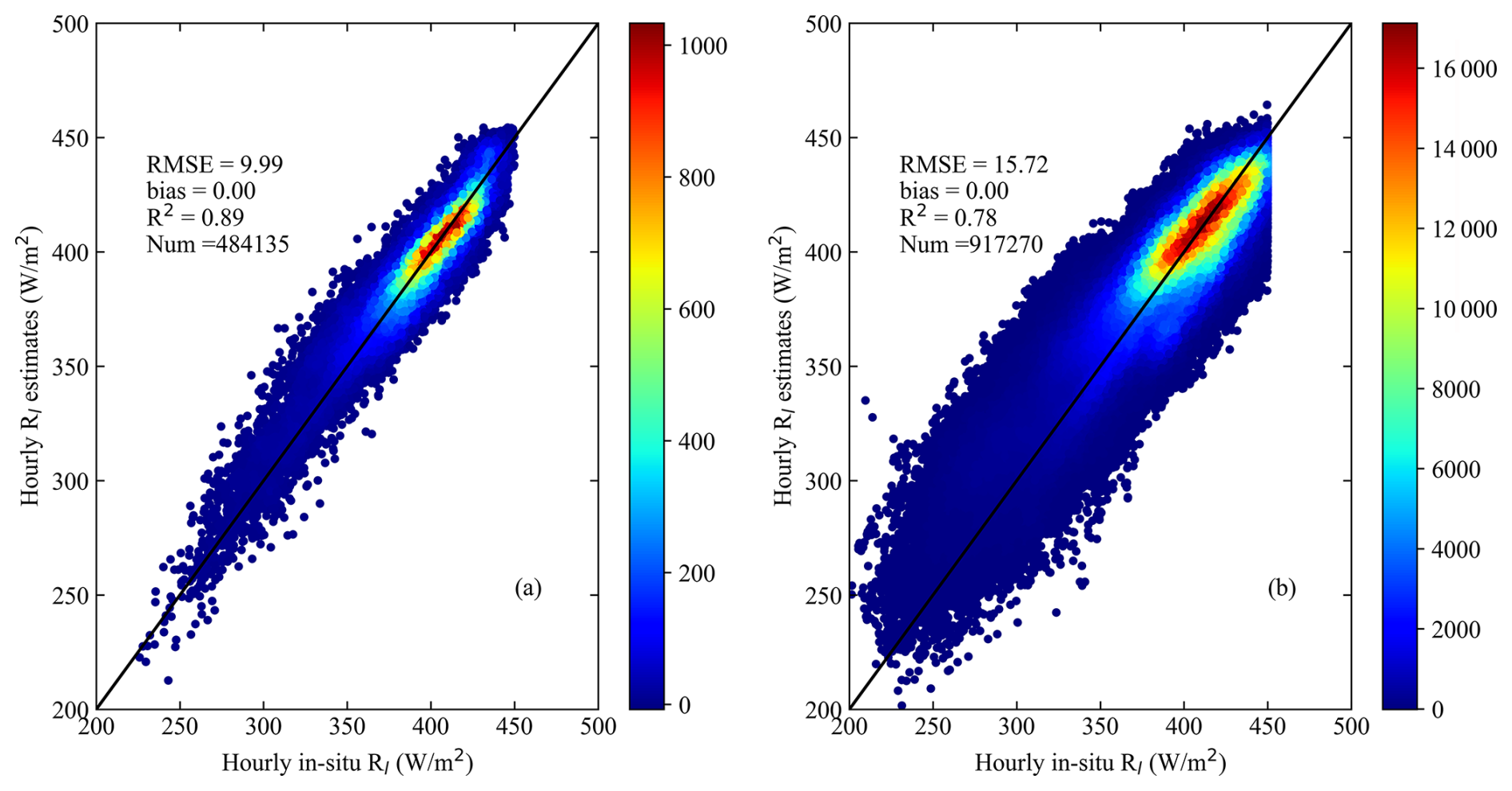
Figure 3 Overall training accuracy of the all-sky daily R_l at (a) daily and (b) hourly scales. In panels (a) and (b), the color bar represents points per unit area.

By considering the influence of the calculated cloud cover on the R_l estimates, the hourly results were separated into daytime and nighttime,, as shown in Fig. 4. The training accuracy of the daytime sample was higher than that during nighttime, with R² values of 0.89 and 0.78 and RMSE values of 13.88 and 16.28 W m⁻², respectively. It was assumed that the larger uncertainties in the hourly ocean-surface R_l during nighttime were possibly due to the estimated cloud cover, which might have an influence on Modnew in the form of overestimating R_l. Overall, the performance of Modnew was very good, both at daily and hourly scales for all-sky R_l estimation at the ocean surface.

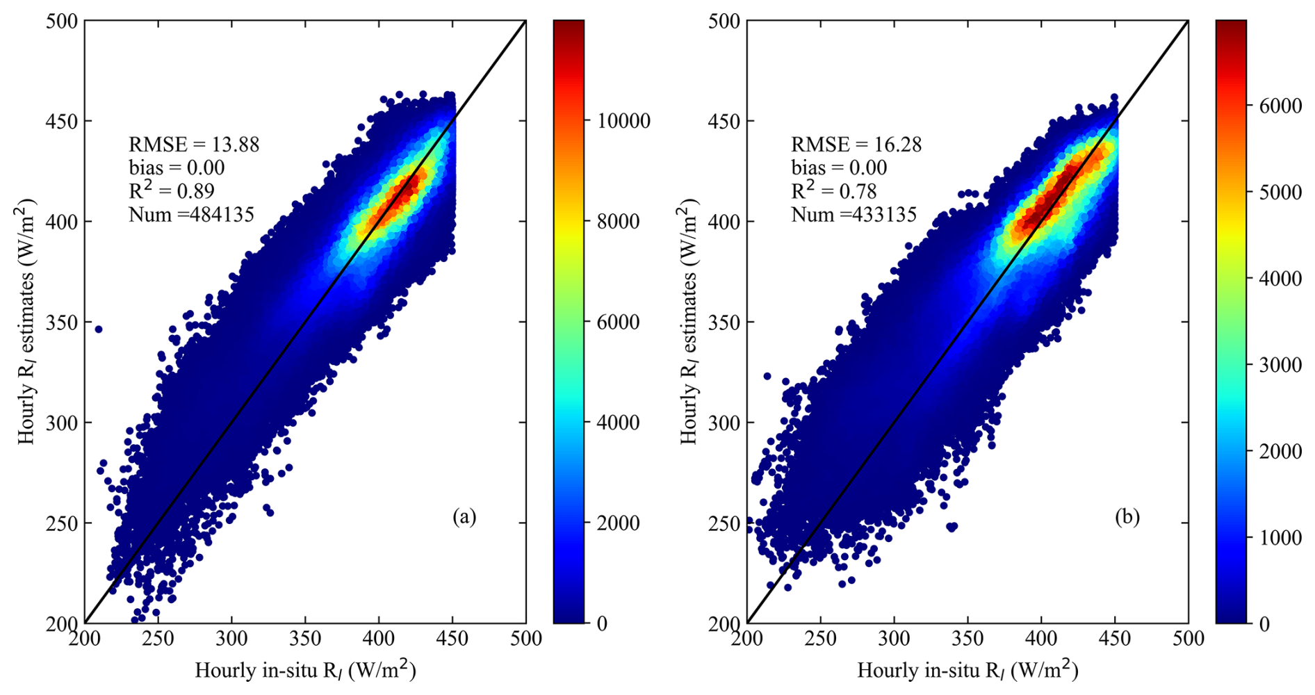
Figure 4 Overall training accuracy of the all-sky hourly R_l during (a) daytime and (b) nighttime. The color bars represent points per unit area.

4.2 Model comparison results

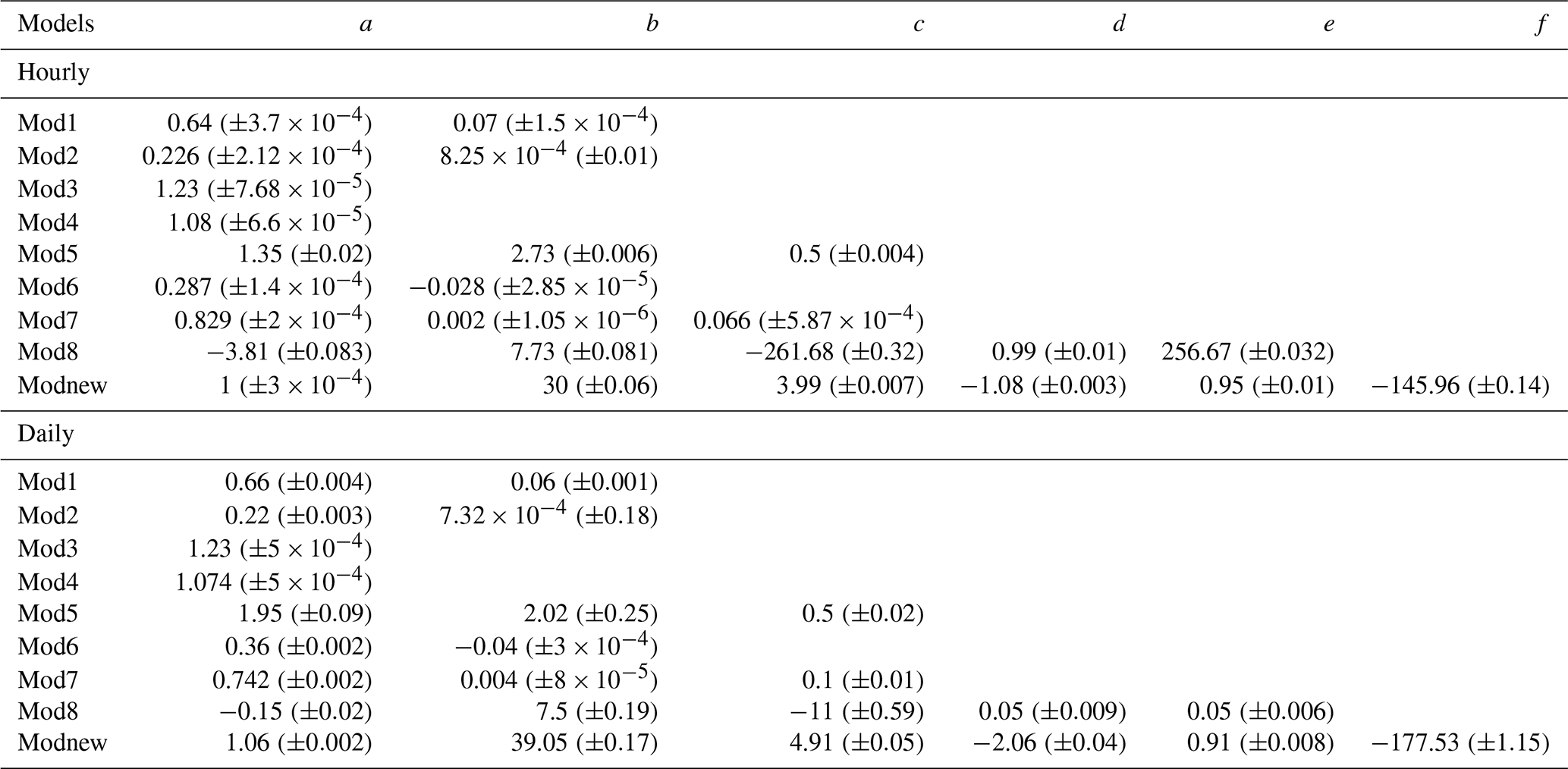
Based on the independent validation samples, Mod1–Mod8 and Modnew were validated one by one and compared for various cases (Table 4). Before that, the eight existing models were calibrated using the corresponding training samples, which means that Mod1–Mod5 were calibrated with the clear-sky training hourly/daily samples, while Mod6–Mod8 were calibrated with the all-sky training hourly/daily samples, i.e., the same as Modnew. Afterwards, these models were validated against the matched validation samples in each case. The updated coefficients of Mod1–Mod8 and the coefficients of Modnew for hourly and daily scales are given in Table 5. For better illustration, the comparison results are presented for clear- and all-sky conditions in the following paragraphs.

Table 5 Coefficients of the nine models used for hourly/daily ocean-surface R_l estimation. The values in parentheses are the uncertainties in the fitted parameters.

4.2.1 Clear sky

All models, including the eight previous models (Mod1–Mod8) and the newly developed model (Modnew), can be used under clear-sky conditions at both hourly and daily scales with the updated coefficients given in Table 5.

Hourly scale

Table 6 shows the validation results of the nine models under clear-sky conditions at the hourly scale. Additionally, the validation results of Mod1–Mod8 with their original coefficients (see Sect. 2) are also presented in Table 6, using the same validation samples for comparison.

Table 6 Overall validation accuracy of the nine ocean-surface R_l models under clear-sky conditions at the hourly scale. The values in parentheses for Mod1–Mod8 are the validation results found using their original coefficients.

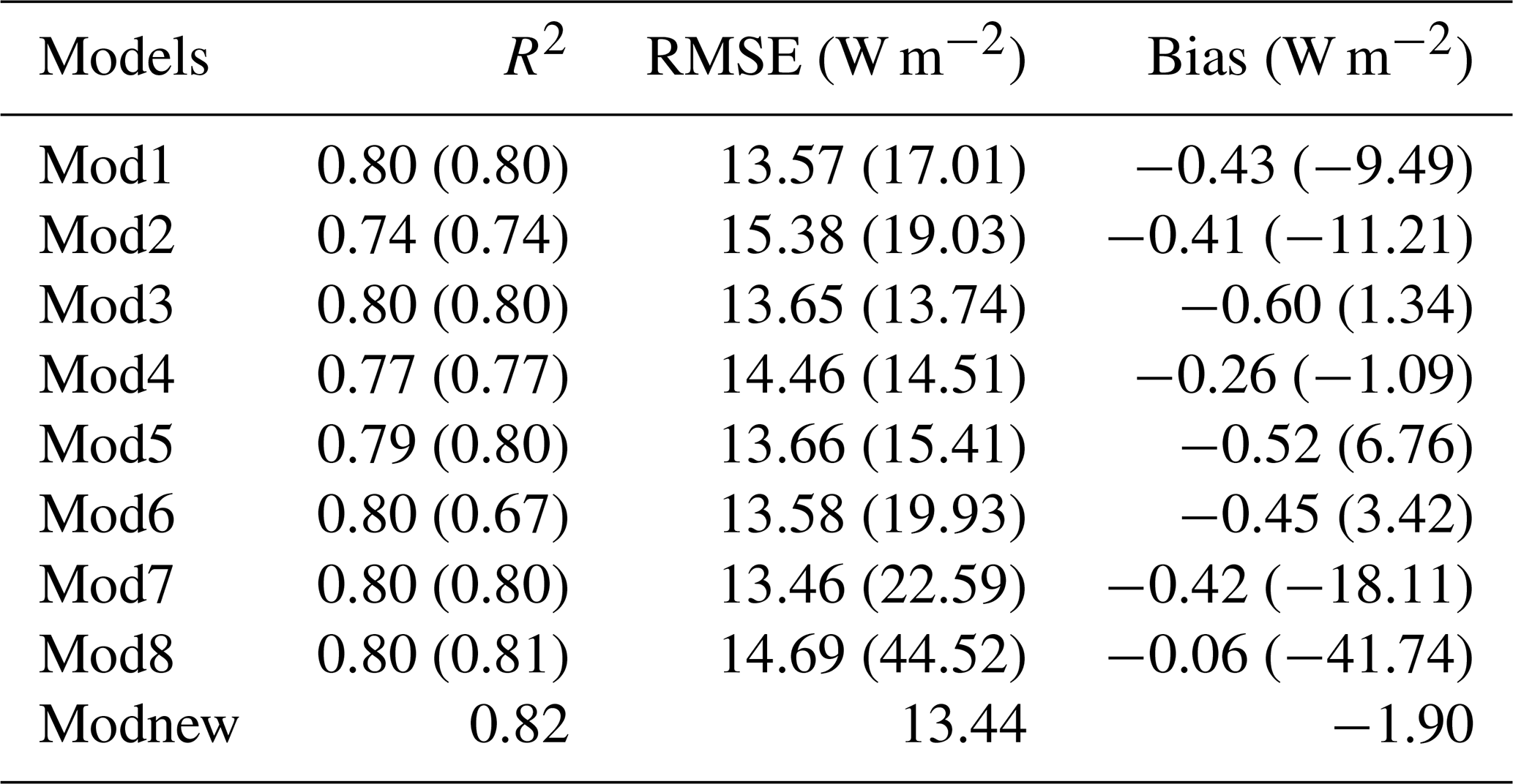
The validation results illustrate that most models estimated the clear-sky hourly ocean-surface R_l with a similar accuracy, with R² values ranging from 0.74 to 0.82, RMSE values ranging from 13.44 to 15.38 W m⁻², and bias values ranging from −1.9 to −0.06 W m⁻² (Table 6). All eight existing models with the calibrated coefficients had a higher accuracy than those with the original coefficients; in particular, the RMSE of Mod8 decreased by ∼ 30 W m⁻². The magnitude of the bias of Mod1–Mod8 also decreased after recalibration, with the magnitude of the biases of Mod1–Mod8 being much smaller than that of Modnew, which was trained with the all-sky hourly samples. Among the nine models, the newly developed Modnew performed the best, with the largest R² of 0.82 and the smallest RMSE of 13.44 W m⁻².

Then, the hourly validation results of the nine models were further examined using the daytime and nighttime values separately, which are shown in Fig. 5. The performance of all models in estimating the hourly clear-sky R_l during the daytime was much better than that during nighttime, with RMSE values during daytime and nighttime ranging from ∼ 12.02 to 14.86 and 14.39 to 17.49 W m⁻², respectively. In addition, among the five clear-sky models, Mod2 – based only on air temperature – shows the lowest accuracy in terms of RMSE during both daytime and nighttime. Among the nine models, Modnew had the most stable performance in hourly R_l estimation under clear-sky conditions during both daytime and nighttime, with similar RMSE values of 12.99 and 14.39 W m⁻², respectively, where its nighttime R_l estimation accuracy in particular was the best among the nine models. However, no accuracy improvement was found when training Mod6 through Modnew using only clear-sky hourly samples.

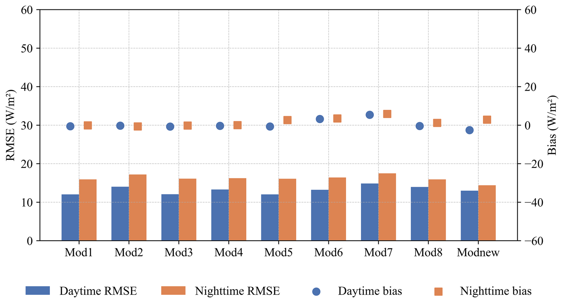
Figure 5 Validation accuracy of the estimated R_l under clear-sky conditions at the hourly scale for the nine models represented by RMSE (left axis) and bias (right axis).

Daily scale

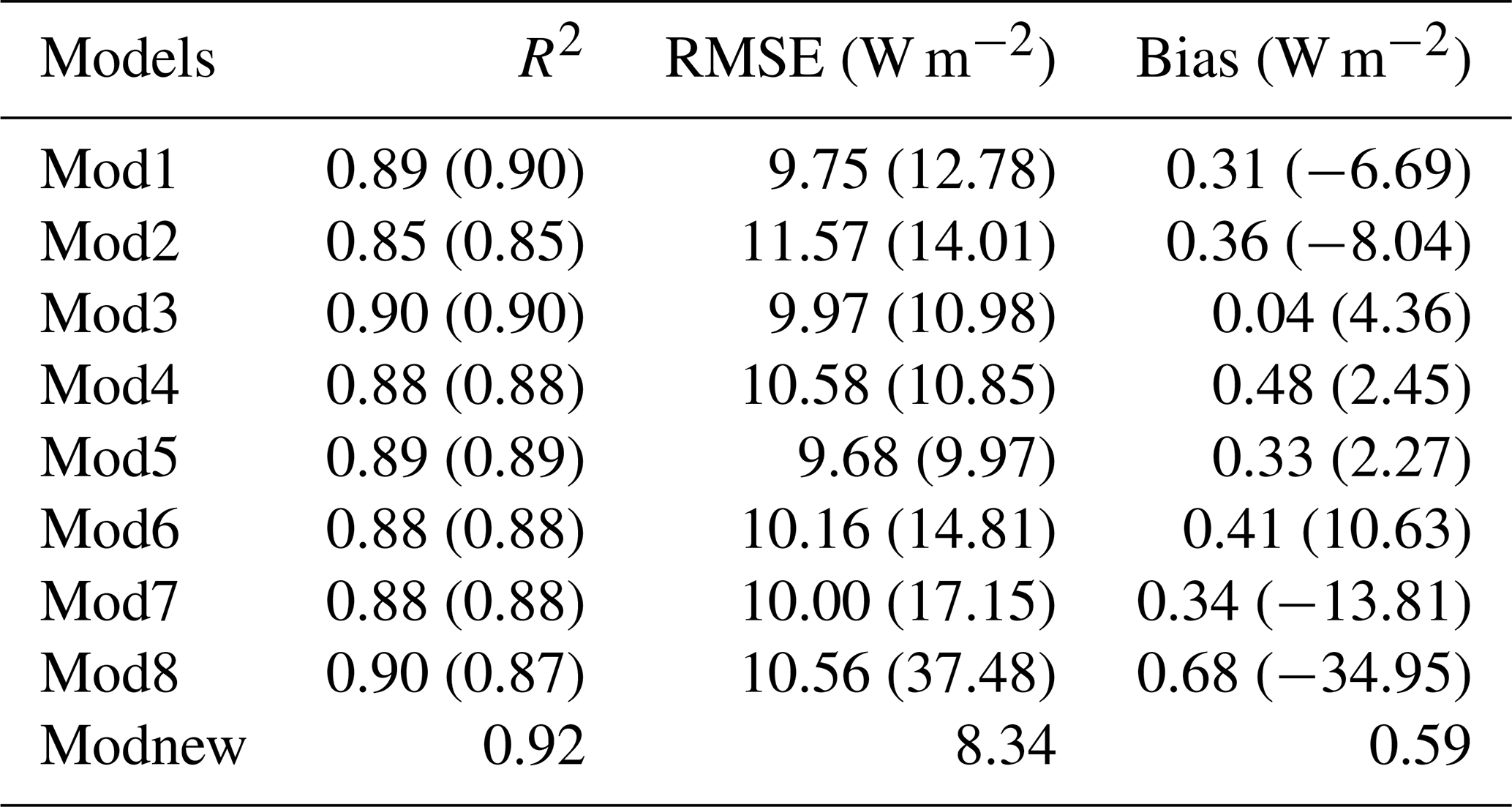
As for the results at the daily scale, the nine evaluated models were trained with the corresponding daily training samples (see Table 4) and validated against the in situ measurements. As shown in Table 7, the estimation accuracy of the daily clear-sky ocean-surface R_l from nearly all previous models improved significantly after recalibration, where the RMSE values and the magnitudes of the bias decreased by up to ∼ 4 and ∼ 10 W m⁻², respectively, except for Mod7. Mod2 still exhibited lower accuracy than the other four clear-sky models, with the highest validated RMSE value of 11.57 W m⁻². The performance of Modnew was the best among the nine models, with the smallest validated RMSE value of 8.34 W m⁻² and bias of 0.59 W m⁻². Similar to the results at the hourly scale, we did not observe accuracy improvements for Mod6 to Modnew when trained using only clear-sky daily samples.

Table 7 Overall validation accuracy of the nine ocean-surface R_l models under clear-sky conditions at the daily scale. The values in parentheses for Mod1–Mod8 are the validation results found using their original coefficients.

4.2.2 All sky

Hourly scale

Table 8 gives the overall validation results of the all-sky hourly scale ocean-surface R_l from the four models against the independent validation samples with the updated and original coefficients.

Table 8 Overall validation accuracy of four ocean-surface R_l models under all-sky conditions at the hourly scale. The values in parentheses for Mod6–Mod8 are the validation results found using their original coefficients.

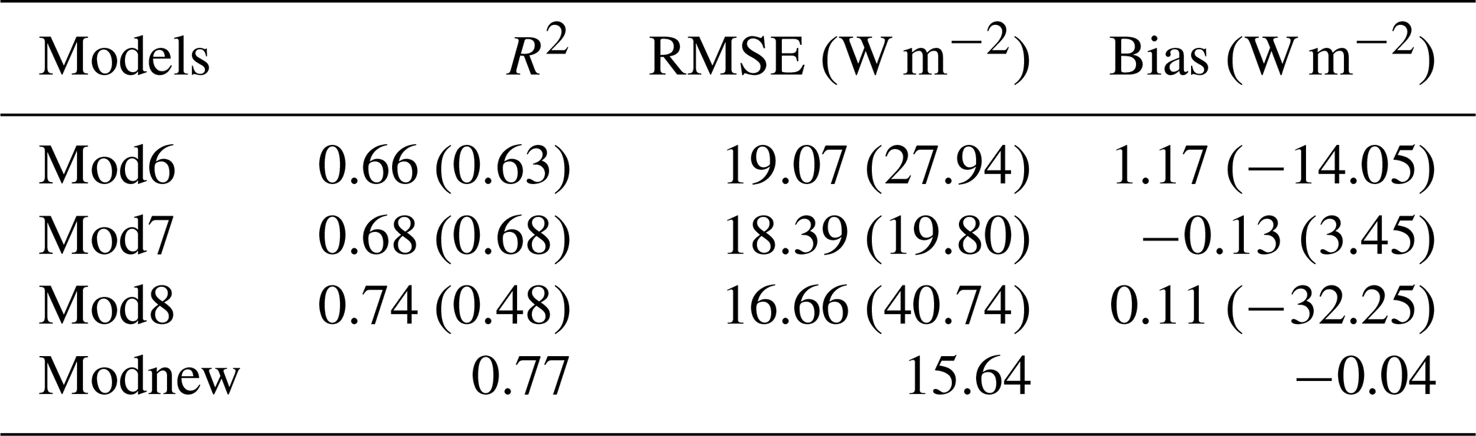
Compared to the results in Table 6, the estimation accuracies under all-sky conditions shown in Table 8 were generally worse, with lower R² values (0.66–0.77) and bigger RMSE values (15.64–19.07 W m⁻²), which indicates that the uncertainty in the cloud information was the major reason for the increased uncertainty in the R_l estimation. As in previous results, the three previous models, Mod6–Mod8, performed much better after recalibration, with decreased RMSE values of up to ∼ 24 W m⁻², and their bias values tended to zero. Modnew performed the best, with an RMSE of 15.64 W m⁻² and a bias of −0.04 W m⁻², followed by Mod8.

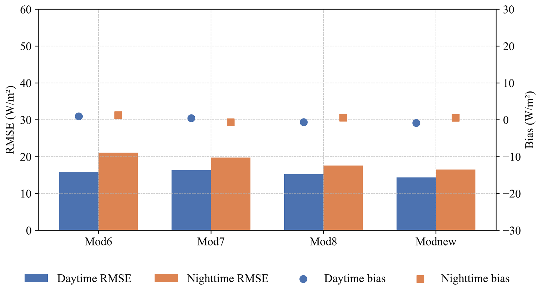
Figure 6 Validation accuracy of the estimated R_l under all-sky conditions at the hourly scale for Mod6–Mod8 and Modnew, represented by RMSE (left axis) and bias (right axis).

The hourly results in Table 8 were examined for daytime and nighttime values, as shown in Fig. 6. The results show that the estimation accuracies of the four models were overall better during the daytime than during nighttime, with smaller RMSE values for the former. Specifically, during daytime hours, the accuracy of Modnew was similar to that of Mod8, with RMSEs of 14.34 and 15.29 W m⁻², respectively, which were better than those of Mod6 and Mod7, which yielded RMSEs of 15.85 and 16.30 W m⁻², respectively. However, Mod7 performed slightly better than Mod6 during the nighttime, although its overall performance was the worst. It is speculated that the larger uncertainties in the all-sky ocean-surface R_l values during nighttime can possibly be attributed to the cloud information during nighttime, which was difficult to estimate accurately compared to the daytime cloud information.

Daily scale

Figure 7 shows the overall validation accuracies of the all-sky daily ocean-surface R_l values from the four models. Compared with Mod6–Mod8, Modnew had the best performance, with a validated RMSE of 10.27 W m⁻², a bias of 0.10 W m⁻², and an R² of 0.88, followed by Mod8, which yielded an RMSE of 11.96 W m⁻², a bias of −0.18 W m⁻², and an R² of 0.85. However, Mod8 had a tendency to overestimate low values (< 300 W m⁻²), as did Mod6 and Mod7.

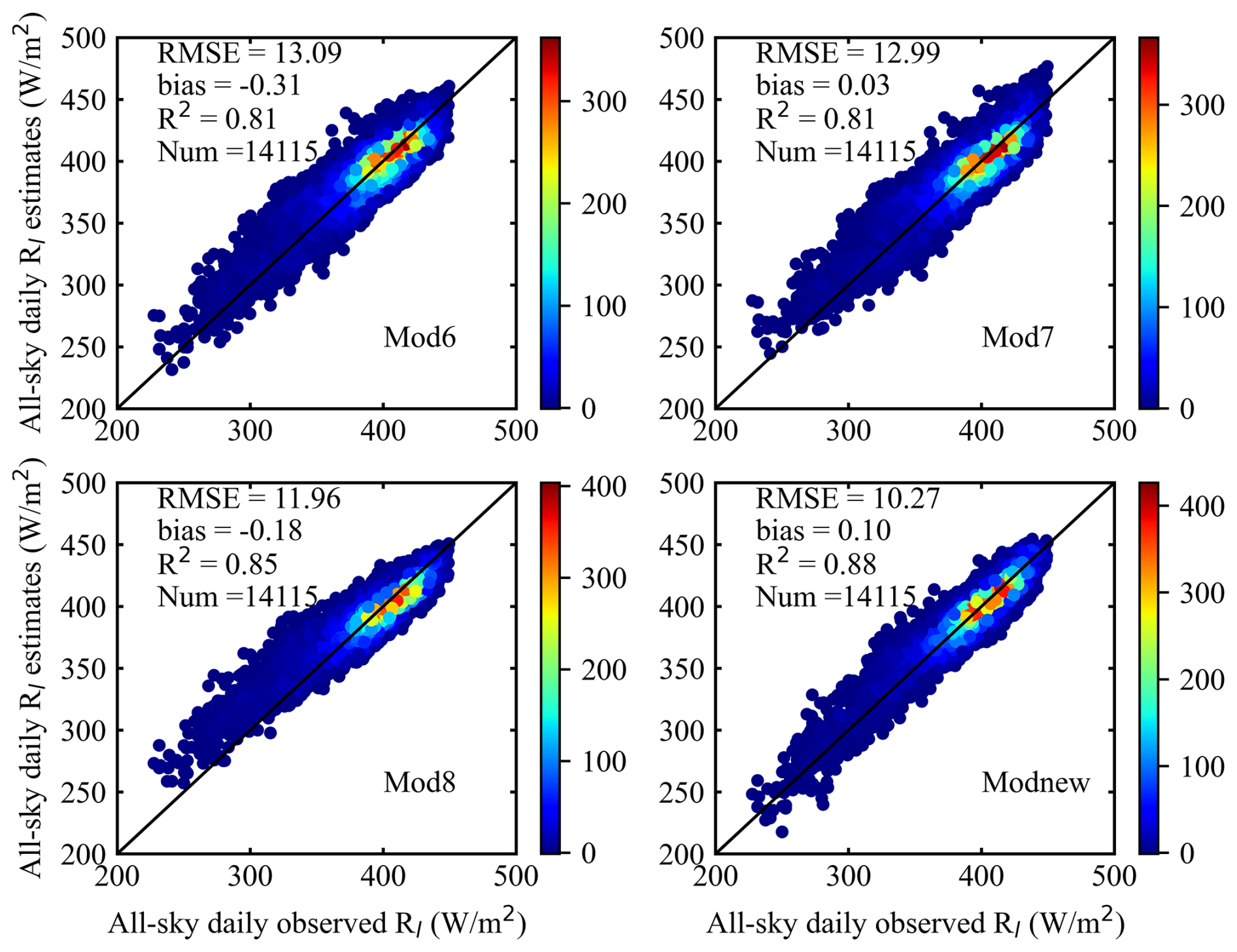
Figure 7 Overall validation results of the calculated all-sky daily ocean-surface R_l from the four models against the independent moored measurements. The color bars represent points per unit area.

Overall, it is speculated that Modnew performed better than Mod6–Mod8 because of the introduction of two cloud-related parameters (clw and ciw) into the model in addition to the cloud fraction. In order to demonstrate this speculation better, the relationship between the estimation errors in the daily all-sky ocean-surface R_l of the four models and clw, which was used to represent the CBH, was further analyzed. The corresponding mean of the estimation errors in the daily all-sky ocean-surface R_l and its SEM for each bin of clw in logarithmic format (in 10 % increments) were calculated, as presented in Fig. 8.

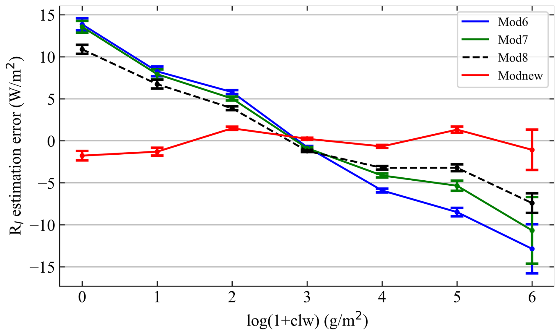
Figure 8 The averaged R_l estimation errors and their SEM of Mod6–Mod8 and Modnew, varied with clw in logarithmic format.

From the results in Fig. 8 it can be seen that the R_l estimation errors of Mod6–Mod8 were negatively linearly related to increasing log (1+clw); such behavior is not seen for Modnew. This indicates that the cloud information related to the variations in daily ocean-surface R_l is not fully characterized by only the cloud fraction. Although Mod8 performed better than Mod6 and Mod7 because of the introduction of the dew point depression to compensate for the difference between the surface temperature and cloud base temperature, the contributions of the cloud base emission to R_l still cannot be thoroughly expressed over the ocean surface. Hence, Modnew performed better than other models because it also takes clw as input. Moreover, ciw was also introduced into Modnew to ensure its robust performance at high latitudes.

4.3 Further analysis on Modnew

Based on the direct validation results described above, Modnew satisfactorily estimated the ocean-surface R_l under both clear- and all-sky conditions at both hourly and daily scales. Hence, further analysis of this new model, such as testing its performance robustness and a sensitivity analysis, was conducted, and the results are given below.

4.3.1 Modnew performance analysis

In order to examine the robustness of its performance, the spatial distributions of the validation accuracies of the all-sky R_l estimates from Modnew at the moored buoy sites are presented in Fig. 9a–b for hourly and daily scales, respectively. Note that the moored buoy data with fewer than 50 validation samples were excluded to provide a more objective comparison.

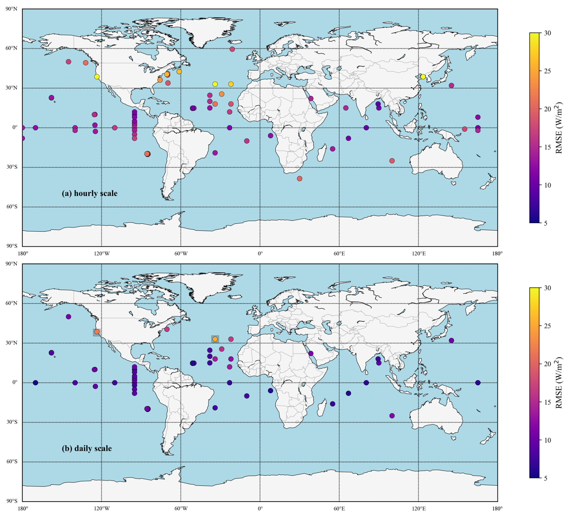
Figure 9 Validation accuracies of Modnew on the hourly scale (a) and daily scale (b) at different sites represented by the RMSE values. The two moored buoys in the shaded boxes in panel (b) are UOP_SMILE88 (38° N, 123.5° W) and UOP_SUB_NW (33° N, 34° W).

The spatial distribution of the validation accuracy (represented by RMSE) of the R_l estimates from Modnew was similar for the hourly and daily data. Modnew's RMSE values increased from tropical to high-latitude seas, although the daily R_l estimates were generally more accurate than the hourly ones, and the validation accuracy for sites at open seas was more accurate than that within coastal seas. For a better illustration, two time series of the estimated daily ocean-surface R_l from Modnew at two sites were randomly selected and are shown in Fig. 10, and the one from Mod8 was added for comparison, with corresponding scatter plots. The two buoys, TAO_03 (0° N, 140° W) and OS_PAPA (50° N, 145° W), are in equatorial and mid- to high-latitude seas, respectively. The temporal variations in the all-sky daily R_l estimates from the two models both captured the variations in the moored R_l measurements very well, but the ones from Modnew were closer to the measurements at high and low values, especially at the OS_PAPA site. The validation accuracy of Modnew was higher than that of Mod8 at both sites, and Modnew performed better in tropical seas, with validated RMSE values of 6.76 and 10.21 W m⁻², respectively. This was assumed to be due to more samples used for modeling being collected in tropical seas, which may have influenced the model's performance in mid- to high-latitude seas.

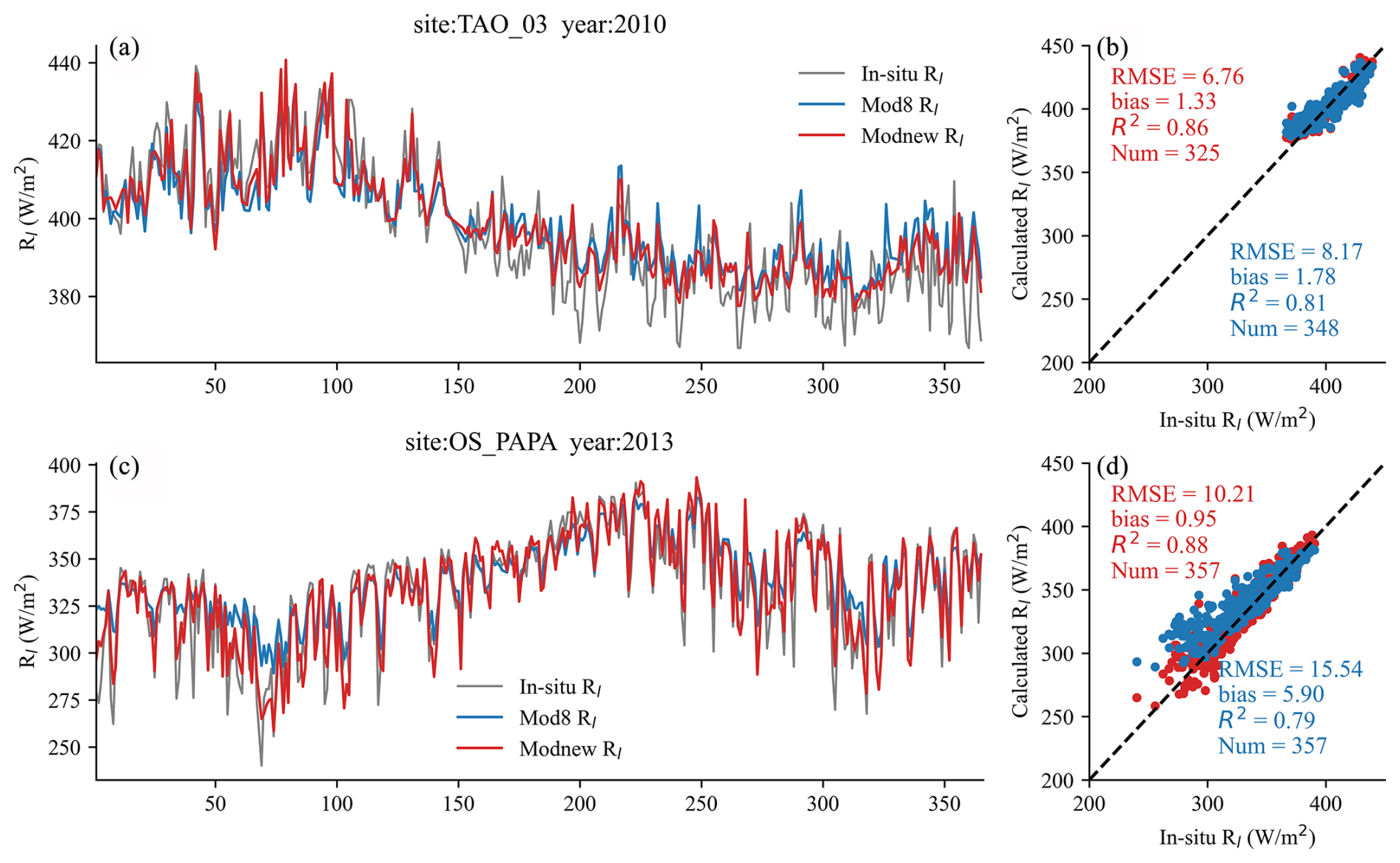
Figure 10 Time series and scatter plots of the R_l estimates and the moored R_l measurements at the (a–b) TAO_03 (0° N, 140° W) and (c–d) OS_PAPA (50° N, 145° W) sites. The red points and blue points represent Modnew and Mod8, respectively.

However, it was noted that Modnew performed poorly at some sites, such as UOP_SMILE88 (38° N, 123.5° W) and UOP_SUB_NW (33° N, 34° W) (see the shaded boxes in Fig. 9). The estimation errors in the daily R_l from Modnew at the two moored buoys were calculated, as shown in Fig. 11, and the ones from the other three all-sky models, Mod6–Mod8, are shown for comparison. It can be seen that the four evaluated all-sky models all performed poorly at the two sites, all giving overestimations. A possible explanation may be the differences in the characteristics of the atmospheric boundary layer over the two sites relative to the open sea. Specifically, UOP_SMILE88 is deployed on the northern Californian shelf, which is influenced by air temperature inversions (ATIs) (Dorman et al., 1995), and UOP_SUB_NW is deployed near the eastern flank of the Azores anticyclone system (Moyer and Weller, 1997). As such, the atmospheric conditions of the two sites are different from those over the open sea, which would affect the estimation of R_l made with models whose coefficients were determined by samples collected mostly from sites located in the open sea. Therefore, more samples should be collected within these seas to help improve the ocean-surface R_l estimation accuracy in these areas.

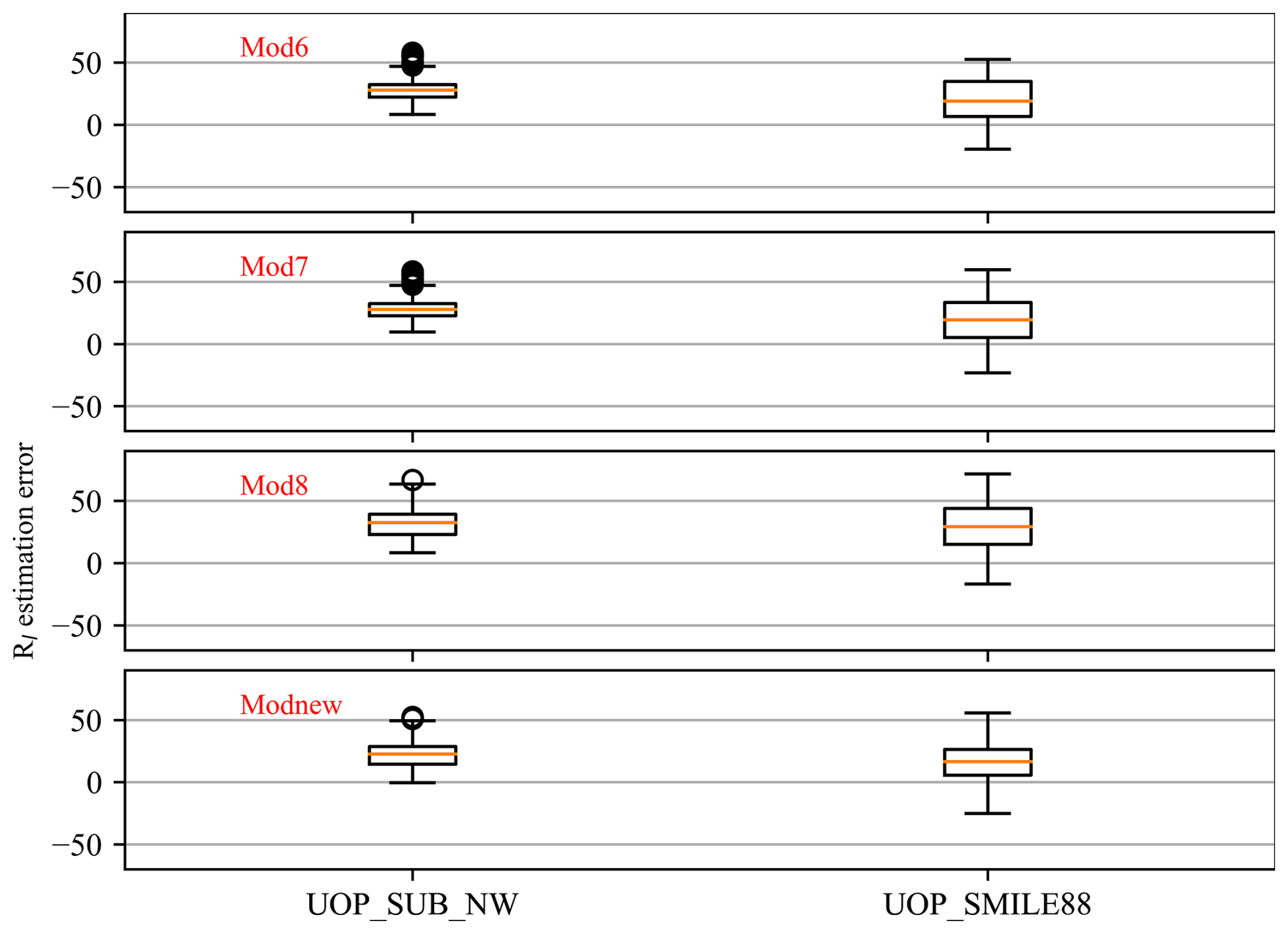
Figure 11 Box plots of the R_l estimation errors from Mod6, Mod7, Mod8, and Modnew at UOP_SMILE88 (38° N, 123.5° W) and UOP_SUB_NW (33° N, 34° W). The top edge, center, and bottom edge of the box represent the 75th, 50th (median), and 25th percentiles, respectively. The whiskers indicate the maximum and minimum values within 1.5 times the interquartile range (IQR), and the circles denote outliers.

4.3.2 Sensitivity analysis

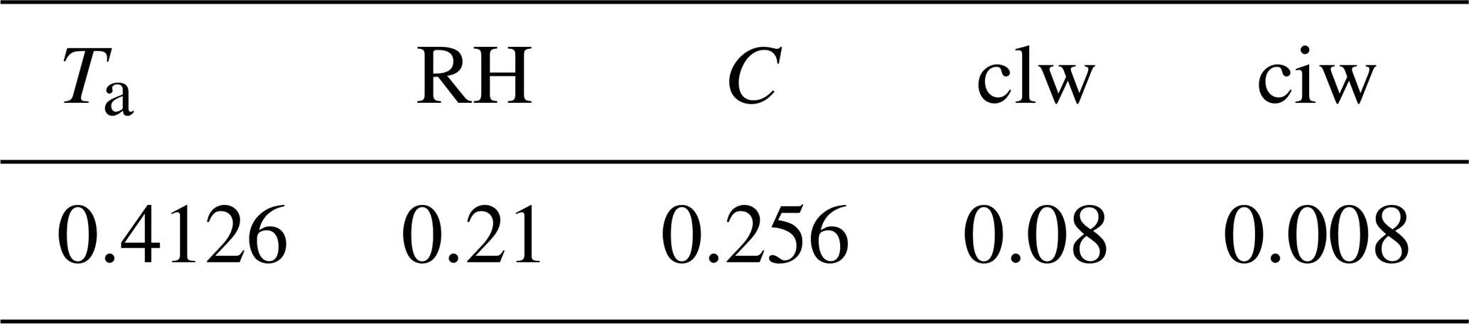
In order to quantify the impact of each parameter on the calculated R_l in Modnew, SimLab software (http://simlab.jrc.ec.europa.eu, last access: 20 April 2020) was used to conduct a global sensitivity analysis. All inputs in Modnew (T_a, RH, C, clw, and ciw) were entered into the software separately, and 2000 ocean-surface R_l values were then calculated using Modnew by taking 2000 combinations of these parameters as inputs. Afterwards, the Fourier amplitude sensitivity test (FAST) method (Saltelli et al., 1999) in the SimLab software was employed to conduct a sensitivity analysis based on the inputs, and the corresponding estimated R_l values were used for a sensitivity analysis using the total sensitivity index (TSI). The TSI indicates each parameter's total contribution to the output variance when the interactions of other parameters are also considered, and it was used to quantify the sensitivity of each parameter. Table 9 shows the TSI of each parameter in Modnew. Specifically, T_a had the most important effect on R_l, with the largest TSI of 41.26 %, followed by C (25.6 %) and RH (21 %). Therefore, the performance of Modnew mainly depended on the accuracy of T_a, C, and RH. The TSI of clw was the fourth highest with 8 %, but it is essential to supplement cloud information that cloud cover alone cannot provide, especially for cloudy-sky conditions. In terms of ciw, its TSI was just 0.008, which was possibly because only a few samples at high-latitudes were used in this study.

Table 9 FAST sensitivity indices of the first order for each input variable in Modnew.

5 Conclusions

Due to the significance of R_l at the ocean surface, many empirical models have been established for ocean-surface R_l calculation based on observations by relating R_l to some climatic factors, such as T_a and RH. However, most models were developed only for clear days, and among those capable of calculating all-sky R_l, only cloud cover is taken into account, which is thought to be insufficient for characterizing the influence of clouds on R_l, especially for ocean surfaces where cloudy skies are common. Indeed, most previous R_l estimation models were developed only within a specific region based on limited observations, and some were developed exclusively for land surfaces. Consequently, there is a need to perform comprehensive evaluations of these models, including their ability to predict R_l over global seas.

In this study, the newly developed Modnew model estimates all-sky ocean-surface downward longwave radiation (R_l) by incorporating key atmospheric and cloud parameters: screen-level air temperature (T_a), relative humidity (RH), fractional cloud cover (C), total column cloud liquid water (clw), and total column cloud ice water (ciw). T_a governs the thermal radiation emitted by the atmosphere, as described by the Stefan–Boltzmann law. RH modifies the atmospheric emissivity by representing the water vapor content. C quantifies the cloud's overall presence, while clw and ciw capture the thermal contributions of liquid and ice clouds, respectively, enabling a more accurate characterization of cloud radiative effects. The Modnew model relies on specific atmospheric and cloud-related parameters for accurate R_l estimation. While inputs such as T_a and RH are commonly obtained from in situ measurements, critical cloud-related parameters (i.e., clw and ciw) are typically derived from satellite products or reanalysis data sets, such as ERA5. These parameters are essential for capturing the radiative properties of clouds, which in situ measurements alone cannot reliably provide. Therefore, satellite data or reanalysis products are indispensable for supplying these inputs. This model, as well as eight comparison models, was used to estimate the all-sky ocean-surface R_l at both hourly and daily scales based on comprehensive observations collected from 65 globally distributed moored buoys from 1988 to 2019. In contrast to previous models, Modnew incorporates more cloud-related parameters (i.e., clw and ciw) into the model in addition to just cloud cover. Modnew and the eight previous R_l models were assessed against the moored values in various cases, including clear- and all-sky conditions during daytime and nighttime and at hourly and daily scales. After careful analysis, several major conclusions can be drawn:

• 1.

  The eight previous models performed much better after calibration of their coefficients with the global observations in almost all cases, except Mod7 in some situations.

• 2.

  For the clear-sky ocean-surface R_l estimation, all models performed better during daytime than during nighttime. Among all models, Modnew was the most robust, yielding RMSE values of 12.99 and 14.39 W m⁻² during daytime and nighttime for the hourly scale, respectively.

• 3.

  For the all-sky ocean-surface R_l estimation, the performance of the four evaluated models was generally worse compared to that under clear-sky conditions, which further demonstrated that the uncertainty in the all-sky R_l estimation was highly dependent on accurate cloud information. Specifically, at the hourly scale, the validated RMSE values of the four models ranged from 15.64 to 19.07 W m⁻², with better performance during daytime. At the daily scale, the RMSE values ranged from 10.27 to 13.09 W m⁻². Modnew also performed the best in these cases, with an overall validated RMSE of 15.64 and 10.27 W m⁻² and bias values of −0.04 and 0.10 W m⁻², respectively. It is worth noting that Modnew performed similarly during both daytime and nighttime at the hourly scale.

In summary, the performance of Modnew was superior to that of previous models for ocean-surface R_l estimation in all cases, which was mainly because of the introduction of more cloud-related information (clw and ciw). Further analysis of Modnew illustrated the significance of the two parameters and cloud cover. However, all results again emphasized that the accuracy of nearly all the empirical models was highly dependent on the spatial distribution, quality, and quantity of the samples used for modeling. For instance, Modnew performed better in open seas in tropical regions where more samples were available compared to other regions. Therefore, many more samples at different regions, such as in coastal regions and high-latitude seas, should be collected in the future to improve model performance. Moreover, more accurate cloud information, especially during nighttime, is essential to decrease the uncertainty in the estimated R_l at the ocean surface.