Practical guidelines for reproducible N₂O flux chamber measurements in nutrient-poor ecosystems

The atmospheric concentration of nitrous oxide (N₂O) has increased significantly since 1800, mainly due to agricultural activities. However, due to their large area, nutrient-poor natural soils, including those in the (sub-) Arctic, also play a crucial role in N₂O emissions and consumption. Despite their importance, these soils have been understudied, due to methodological limitations in detecting low fluxes. Our study addresses this knowledge gap by testing a fast-responding portable gas analyser (PGA; Aeris MIRA Ultra ${\mathrm{N}}_{\mathrm{2}}\mathrm{O}/{\mathrm{CO}}_{\mathrm{2}}$) combined with manual chambers (height and diameter: 25 cm) for measuring N₂O fluxes from a nutrient-poor, sub-Arctic peatland. Our results show that this setup can detect and quantify low N₂O flux rates, with a mean and standard error of $-\mathrm{0.61}\pm \mathrm{0.08}$ µg N₂O-N ${\mathrm{m}}^{-\mathrm{2}}{\mathrm{h}}^{-\mathrm{1}}$ for a 5 min closure time, as observed in our study. More than 70 % of the measured N₂O fluxes exceeded the minimum detectable flux ($\mathrm{0.027}\pm \mathrm{0.0002}\mathrm{\mu }\mathrm{mol}{\mathrm{m}}^{-\mathrm{2}}{\mathrm{h}}^{-\mathrm{1}}$), which varied according to chamber closure time. Our study highlights the importance of using fast-responding analysers to measure low N₂O fluxes and improve our understanding of diverse N₂O flux dynamics. For nutrient-poor soils, we recommend a chamber closure time of approximately 5 min. We also found that a non-linear flux calculation model yielded better results and was broadly applicable, including cases where data were linearly distributed. Overall, our study demonstrates the potential of fast-responding analysers to improve our understanding of N₂O flux dynamics in nutrient-poor soils.

1 Introduction

Nitrous oxide (N₂O) is the third most important greenhouse gas (GHG), with a global warming potential almost 300 times stronger than carbon dioxide (CO₂) over a period of 100 years (IPCC, 2023). It stays in the atmosphere for around 110 years, and its atmospheric concentration has increased from 273 to 336 ppb since 1800 (Lan et al., 2022). As most of this increase can be attributed to human activities, particularly the use of nitrogen (N) fertilisers in agriculture, research has focused on N₂O emissions from managed agricultural soils (De Klein et al., 2020), which hold the potential for high N₂O emissions. This is because the input of N increases the readily available mineral N needed for plant growth and thus increases harvests but, simultaneously, can also result in higher N₂O emissions (Myhre et al., 2013).

Until about 15 years ago, few studies investigated N₂O fluxes in the (sub-) Arctic, where soils often have a very low availability of reactive N (Virkkala et al., 2024) and thus are not expected to emit amounts of N₂O relevant for the global climate (Voigt et al., 2020; Christensen et al., 1999; Grogan et al., 2004; Martikainen et al., 1993). In these low N ecosystems, N₂O uptake could be expected but has, so far, not been confirmed in field studies (Buchen et al., 2019; Schlesinger, 2013). Since 2009, multiple studies have reported N₂O emissions similar to agricultural soils from organic-rich ecosystems in the Arctic (Repo et al., 2009; Marushchak et al., 2011; Elberling et al., 2010), shifting the focus to only selected high-nutrient areas within the (sub-) Arctic. Nevertheless, reporting near-zero N₂O fluxes is crucial to avoid overestimating emissions caused by biased site selection favouring high-emitting areas (Voigt et al., 2020).

In most studies, N₂O concentrations were sampled repeatedly with a syringe from the head space of a closed flux chamber and measured with a gas chromatograph (GC) in the laboratory (Hensen et al., 2013; Denmead, 2008; Pavelka et al., 2018). With this approach, typically between four and six discrete air samples are taken to measure N₂O mixing ratios during the chamber closure time and calculate the fluxes. The sensitivity of GCs varies but, with only a few samples drawn from a fluctuating time series that may not necessarily display a linear trend, differences in low concentrations are hard to capture and highly dependent on single data points (Hübschmann, 2015). Additionally, in previous studies, opaque chambers have mostly been used because temperature inside the chamber would increase less above the ambient temperature, compared with transparent chambers (Clough et al., 2020). As a result, there are only a few studies investigating N₂O fluxes under different light conditions (Stewart et al., 2012). Since this was the only available method for in situ N₂O measurements in the field, our knowledge on (sub-) Arctic N₂O fluxes is rather limited and this makes it challenging to establish accurate baseline estimates, which are essential for detecting changes in fluxes.

Recent advances in laser spectroscopy led to novel, portable (<15 kg), and fast-responding (1 Hz, i.e. sampling every second) GHG analysers, offering new possibilities for measuring low N₂O concentrations in nutrient-poor ecosystems (Subke et al., 2021). These portable gas analysers (PGAs) allow near-continuous monitoring of concentration changes, providing higher precision and lower detection limits than GC-based methods (Hensen et al., 2013). While differences in flux estimates between PGAs and GCs have been well-documented for CH₄ and CO₂, few studies have focused on N₂O (Christiansen et al., 2015; Brümmer et al., 2017). The detection limit was a significant constraint, as many reported N₂O fluxes were below the threshold of the GC method, limiting the ability to accurately assess their magnitudes and trends. The availability of PGAs for in situ N₂O flux measurements raises new methodological questions. Unlike CH₄ and CO₂, where, for a fixed chamber height, approximately 3 min periods are well-accepted for reliable measurement, the minimum chamber closure time for N₂O fluxes in nutrient-poor ecosystems is unclear. This is because N₂O concentrations are very low and take longer to accumulate in the chamber head space to accurately detect trends (Fiedler et al., 2022). Few studies have investigated the chamber closure time with portable N₂O analysers, and the reported recommendations range between 3 and 10 min and originate from ecosystems with higher N₂O flux rates (Fiedler et al., 2022; Brümmer et al., 2017).

The chamber community has been discussing the use of linear (LM) or non-linear (HM) models to calculate flux rates for decades (Pumpanen et al., 2004). The critique on the linear models is that they underestimate the flux rates due to the assumption that GHG concentrations keep increasing within the chamber head space (Fiedler et al., 2022; Hüppi et al., 2018). However, it is clear from the theory of molecular diffusion that the rate of concentration change within the chamber declines over time (Hutchinson and Mosier, 1981; Kutzbach et al., 2007; Kroon et al., 2008). As a result, there have been great efforts to implement non-linear flux calculations as alternatives to LM models, for example, through software packages (Pedersen et al., 2010; Hüppi et al., 2018). However, non-linear flux calculations are not commonly used in the chamber community, probably because they are more complex to implement. For N₂O, there is a lack of data sets from nutrient-poor ecosystems to evaluate the effect of LM and HM models.

The main aim of this paper is to present a mobile flux chamber method capable of quantifying (very) low N₂O fluxes in nutrient-poor ecosystems. Using a novel portable N₂O analyser (Aeris MIRA Ultra ${\mathrm{N}}_{\mathrm{2}}\mathrm{O}/{\mathrm{CO}}_{\mathrm{2}}$) and our custom-made transparent and opaque flux chambers, we provide the first extensive data set of low N₂O fluxes from the (sub-) Arctic. We tested the performance of our PGA in the laboratory and in the field across various land cover types from a thawing permafrost peatland in sub-Arctic Sweden. We compared N₂O flux rates calculated from different chamber closure times (3–10 min) and evaluated differences between linear and non-linear calculation methods. Additionally, we compared flux rates based on high-frequency in situ observations against an approach that randomly draws discrete data points from the full time series, mimicking a GC-based approach. Finally, we aim to provide guidance on measuring N₂O fluxes in nutrient-poor ecosystems, such as the Arctic. Ideally, this will encourage researchers to measure low fluxes in (sub-) Arctic regions, get a better process understanding of N₂O fluxes, and determine how the N cycle in nutrient-poor ecosystems will respond to Arctic warming.

2 Methods

To facilitate the reader's understanding, we use the terminology proposed by Fiedler et al. (2022), with location describing the area where sampling occurs (“Stordalen mire”), site describing a vegetation unit within the location (“palsa lichen”, “palsa moss”, “bog”, “fen”), and chamber base position (i.e. plot) indicating the exact spot where N₂O was measured. By “chamber closure time”, we specify the time frame in which a chamber was closed onto the soil; one of these periods is then called a “measurement period”.

2.1 Study location and sampling sites

All data were collected at the Stordalen mire, a complex palsa mire underlain by sporadic permafrost located in sub-Arctic Sweden (68°20.0^′ N, 19°30.0^′ E), 10 km east of Abisko (Ábeskovvu in Northern Sámi language). Permafrost has been rapidly thawing at this location over the last decades, and only remains in the dry uplifted areas on the peatland (palsas) (Sjögersten et al., 2023). For our study, we randomly selected 24 chamber base positions in three transects on a dry-to-wet thawing gradient from palsa to bog to fen, with six replicates for each land cover type: palsa lichen, palsa moss, bog, and fen (Fig. 1). Transects 1 and 2 each contain six chamber base positions and are located in the northern centre of the mire, within the footprint of an integrated carbon observation system (ICOS, SE-Sto) eddy covariance tower, which has been operating since 2014 (Lundin et al., 2025, Fig. 1). Transect 3 lies in the most north-eastern part of the palsa.

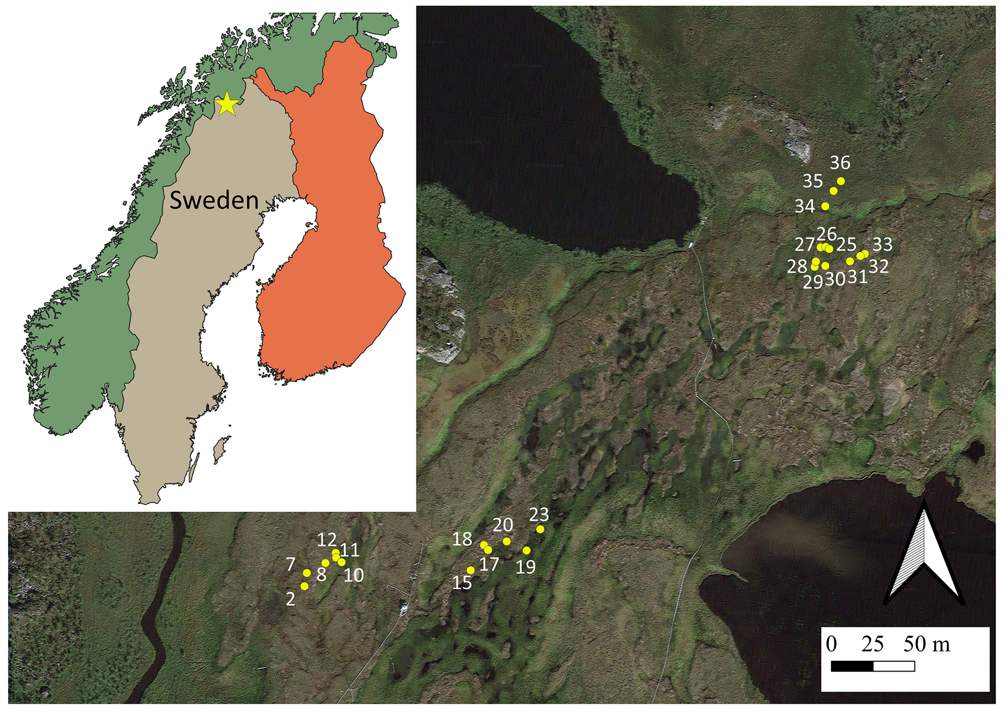
Figure 1 Three transects with chamber base positions in Stordalen overlaid on satellite image from © Google Maps. The location of the Stordalen mire is marked with a star. Here, micro habitats are represented with different colours and symbols for clarity. The spatial data of each country can be found at https://simplemaps.com, last access: 17 September 2024.

Vegetation on the palsa is mainly dominated by lichen (Cladonia spp.), shrubs (Empetrum nigrum hermaphroditum, Betula nana, Vaccinium uliginosum, Vaccinium vitis-idaea, Rubus chamaemorus), and some mosses (Dicranum elongatum, Sphagnum fuscum). Both bogs and fens contain peat-forming mosses (Sphagnum balticum, Sphagnum lindbergii, Sphagnum riparium), with the dominant vascular plants on fens being cotton grass (Eriophorum vaginatum, Eriophorum angustifolium) and that in bogs being sedges (Carex rotundata, Carex rostrata). The soils in the area are classified as organic histosols or, if permafrost occurs within 2 m of cryoturbation activities, as cryosols (Siewert, 2018). Research at the Stordalen mire has been conducted for over a century (Jonasson et al., 2012; Callaghan et al., 2013) and a vast amount of data on CH₄ and CO₂ fluxes has been published (Łakomiec et al., 2021; Varner et al., 2022). The mean annual temperature at the Stordalen mire is −0.6°C and the annual precipitation is 304 mm (Malmer et al., 2005).

The data presented in this study were collected during three separate campaigns covering different seasons: spring (23–30 May 2023), summer (20–27 July 2023), and autumn (3–22 September 2023). PVC collars with an inner diameter of 245.1 mm, a height of 150 mm, and a wall width of 4.9 mm were inserted into the soil on 29 August 2022. We inserted them as deeply as possible, between 100–140 mm, to ensure a proper seal between the chamber head space and the atmosphere, even during strong wind conditions, and in the palsa, where the top peat was dry and highly porous. Between the collar and the chamber, we placed a custom-made sealing ring to avoid ambient air entering the chamber during our measurements (Fig. 2 and Fig. S2 in the Supplement). The sealing ring has inner and outer diameters of 235 and 265 mm, respectively, and a height of 30 mm and is built from a metal ring wrapped in foam material (50 mm on each side). Tests confirmed that it sealed the chamber and the collar, even under high wind conditions with up to 18 m s⁻¹ wind gusts.

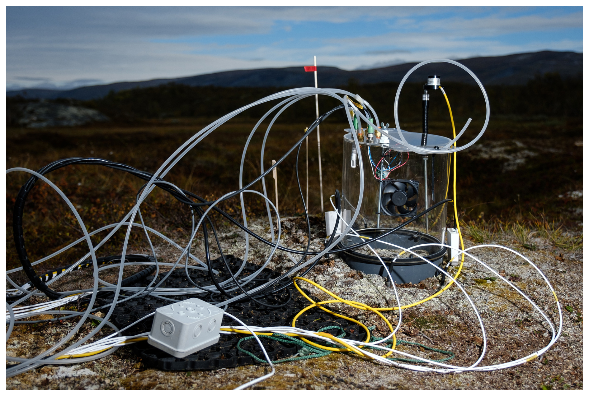
Figure 2 Chamber setup during measurement period, with soil moisture and soil temperature sensors installed in the soil and all inlets connected. Photo: Fabio Cian, “Ubiquitous Anomaly”, CC BY-NC-ND 4.0.

2.2 Chamber and portable gas analyser (PGA) setup and protocol

For our measurements, we used a custom-built static, non-steady-state, non-flow-through chamber (Livingston and Hutchinson, 1995) made from acrylic glass (Göli GmbH) with a height of 250 mm and a diameter of 250 mm (Figs. 2 and S1). We placed a fan (SUNON Maglev, $\mathrm{80}\mathrm{mm}\times \mathrm{80}\mathrm{mm}\times \mathrm{25}\mathrm{mm}$, 2000 rpm) inside the chamber to ensure well-mixed conditions within the chamber during the measurements. Additionally, we installed a relative humidity (RH) and temperature probe (EE08, E+E Elektronik, Germany) and a pressure sensor (61402V, RM Young) for measuring essential parameters to calculate the fluxes. We equipped the chamber with quick-release connectors on top to connect the inlet and outlet tubing to the portable gas analysers. As complementary variables, we measured soil temperature at 15 cm (PT100 4-wire sensors, JUMO GmbH and Co. KG) at each quadrant outside of the plot, soil moisture at 12 and 30 cm (CS655-DS and CS650-DS, Campbell Scientific), and photosynthetically active radiation (PAR) (PQS1, Kipp and Zonen). More detailed information on our chamber setup can be found in the Supplement.

To measure N₂O concentrations, we used the Aeris MIRA Ultra ${\mathrm{N}}_{\mathrm{2}}\mathrm{O}/{\mathrm{CO}}_{\mathrm{2}}$ (from now onward: Aeris-N₂O) analyser (Aeris Technologies; sensitivity: 0.2 ppb s⁻¹ for CO₂ and N₂O; frequency: 1 Hz). As with most PGAs, the Aeris-N₂O provides dry mole fractions of the target gas. We performed several laboratory tests to assess the signal stability (i.e. drifts and stabilisation time), uncertainties, noise level, and water interference of the Aeris-N₂O. Furthermore, we tested the impact of the humidity on the Aeris-N₂O analyser using a portable dew point generator (LI-610, Licor USA). By adjusting the dew point temperature, we examined four different humidity levels: 28 %, 45 %, 60 %, and 83 %. A calibration gas tank with a known N₂O concentration of 333.2 ppb was first connected to the dew point generator. The humidified gas was then connected to the Aeris-N₂O analyser inlet and each humidity level was sampled for about 20 min. Nevertheless, only a 10 min window was used for further analysis, due to the relatively long time (about 10 min) required for the humidity levels to stabilise (see Fig. A2).

In the field, we attached a custom-made external battery box with two LiFePO₄ batteries (LiFePO₄ 12.8 V 20 Ah, Green Cell) to the Aeris-N₂O, which could be switched whilst the analyser was running. In this study, one LiFePO₄ 12.8 V 20 Ah battery lasted for the whole day of field measurements (8 h to a maximum 12 h). A data logger (CR1000X, Campbell Scientific), which was placed inside a Pelican case (Figs. S3 and S4), was used to log all the sensor data, including greenhouse gas concentrations. All GHGs and explanatory variables were logged with a frequency of 1 Hz. With this setup, all necessary information for the analyses was synchronised in a single data file, rather than many individual files from individual sensors and loggers.

Before we started a measurement period (i.e. the time during which the chamber is closed), we attached the tubes from the PGA to the chamber, ventilated the chamber for at least 1 min, and gently closed it onto the sealing ring. The default chamber closure time for all measurement periods was 10 min. For dark measurements, a custom-made light-impermeable tarpaulin was placed over the chamber to prevent light from entering and minimise temperature fluctuations. We refer to these measurements as “opaque”, for clarity.

All data were processed in R (version 4.3.3; R Core Team, 2024) and version controlled in GitLab (the scripts are publicly available from https://git.bgc-jena.mpg.de/ntriches/data-analysis/-/tags/2024-12-12-triches-amtsubmission-n2oadvances last access: 22 July 2025). A filter script was applied to the data to ensure they met certain quality control standards, including

• removing data from the beginning of each measurement period to account for the time lag of gases moving through the tubes to reach the laser cell

• removing implausible values (e.g. −9999) of chamber pressure, chamber temperature, chamber relative humidity, soil temperature, volumetric water content, and PAR

• replacing negative PAR values with 0

• averaging soil temperature readings gained from four sensors

• detecting and removing flat lines indicating instrument failure (see Sect. S1.3 in the Supplement)

• pre-processing data for concentrations of N₂O, CO₂, and H₂O, as well as other relevant parameters.

2.3 Flux calculations

In our study, we calculated N₂O fluxes using all data points from one measurement period. We removed 8 s worth of data at the start of the measurement period to account for the time delay until the concentration from the chamber reached the cell of the gas analyser. An extra 7 s of data were removed for opaque measurements, since we needed more time in the field to cover the chamber with the reflective tarpaulin. To calculate the fluxes using both linear (LM) and non-linear (HM) methods in a reproducible way, we used the R package goFlux (v0.2.0, Rheault et al., 2024). We selected goFlux for several reasons: (i) it was specifically written to process data gathered with PGAs, (ii) it uses temperature and pressure measured inside the chamber for flux calculation, (iii) it corrects for the dissolved gases in the water vapour inside the chamber, and (iv) it calculates fluxes using both LM and HM flux calculation methods. It also enables the comparison of results from LM and HM models using various statistical methods and flags, such as the minimum detectable flux (MDF, Eq. 4). Additionally, it generates plots for visualisation. For the flux calculation in LM, goFlux applies the commonly used linear equation as follows:

$$\begin{array}{}\text{(1)}& F\left(t\right)={\displaystyle \frac{\mathrm{d}C\left(t\right)}{\mathrm{d}t}}{\displaystyle \frac{V}{A}},\end{array}$$

where F(t) is the gas flux rate at a given location during the chamber closure time (t), $\mathrm{d}C\left(t\right)/\mathrm{d}t$ is the mass concentration change with time, V is the volume of the chamber, and A is the area of the soil covered by the collar (Subke et al., 2021). To report our flux rates, we used the atmospheric sign convention, i.e. negative signs for an uptake of N₂O into the soil and positive signs for emissions.

The HM model approach is based on the approach of Hutchinson and Mosier (1981):

$$\begin{array}{}\text{(2)}& C\left(t\right)=\mathit{\phi }+(C_{\mathrm{0}}-\mathit{\phi }){\mathrm{e}}^{-\mathit{\kappa }t},\end{array}$$

where φ is the assumed constant gas concentration of the source within the soil (Pedersen et al., 2010), C₀ is the gas concentration in the chamber at the moment of chamber closure, and κ is the model parameter. To limit κ with a maximum threshold κ_max, Eq. (3) was adapted from Hüppi et al. (2018):

$$\begin{array}{}\text{(3)}& {\mathit{\kappa }}_{\text{max}}={\displaystyle \frac{F\left(t\right)}{\text{MDF}t}}.\end{array}$$

Here, MDF is a theoretical threshold that represents the instrument's detection limit, based on its precision (η), provided by the manufacturer. However, it does not account for potential errors in the model or chamber artefacts, but reflects the instrument's inherent uncertainty. The MDF can be calculated using

$$\begin{array}{}\text{(4)}& \text{MDF}={\displaystyle \frac{\mathit{\eta }}{t}}\mathit{\theta },\end{array}$$

where θ is a flux term that corrects for the water vapour inside the chamber and converts the flux unit to $\mathrm{\mu }\mathrm{mol}{\mathrm{m}}^{-\mathrm{2}}{\mathrm{s}}^{-\mathrm{1}}$ and t is the measurement time, i.e. the number of measurement points during the measurement period. This was calculated as

$$\begin{array}{}\text{(5)}& \mathit{\theta }={\displaystyle \frac{(\mathrm{1}-C_{{\mathrm{H}}_{\mathrm{2}}\mathrm{O}})VP}{ART}},\end{array}$$

where $C_{{\mathrm{H}}_{\mathrm{2}}\mathrm{O}}$ is the water vapour concentration (in mol mol⁻¹), P is the pressure inside the chamber (in kPa), R is the universal gas constant (in $\mathrm{L}\mathrm{kPa}{\mathrm{K}}^{-\mathrm{1}}{\mathrm{mol}}^{-\mathrm{1}}$), and T is the air temperature inside the chamber (in K).

In the goFlux package, fluxes that are below the detection limit are flagged. Note that, owing to this function, all our flux estimates have their own MDF. The package further implements the so-called g factor (g_f) (Hüppi et al., 2018) to restrict large curvatures of the non-linear flux models, as

$$\begin{array}{}\text{(6)}& g_{\mathrm{f}}={\displaystyle \frac{{\text{HM}}_{\mathrm{F}}}{{\text{LM}}_{\mathrm{F}}}}.\end{array}$$

Here, HM_F and LM_F are the flux values that are calculated by HM and LM models, respectively. In this study, we used a g_f of 4, meaning that the flux calculated by the HM model can be at most 4 times higher than the flux calculated by the LM to avoid a large overestimation of fluxes (Eq. 6). We used this factor because, upon visual assessment, it fit our data best, and has been previously used (Leiber-Sauheitl et al., 2014). We did not use the mean absolute error or the root mean square error to define whether the HM or LM model performed better, since they were very similar among all measurement periods. We also did not use R² as a filter criterion, since low and non-linear fluxes inherently result in low values of R² (Kutzbach et al., 2007).

2.4 Data processing and simulations

We used our openly available script to simulate differences between chamber closure times and GC sampling, as well as the associated sensitivity analysis. We first calculated all fluxes using the original 10 min chamber closure time (prec =0.2, g.limit =4). To see how different closure times affect N₂O fluxes, we shortened the closure time by 1 min at a time, starting from 9 min, and recalculated the fluxes for each new time (e.g. $\mathrm{9}\min =\mathrm{540}\mathrm{s},\mathrm{8}\min =\mathrm{480}\mathrm{s}$, etc.). We compared how chamber closure time affects flux rates during transparent and opaque measurements, and identified the number of fluxes above the minimum detectable flux, based on the goFlux output. While calculating our fluxes, we became aware of one chamber base position acting as a hot spot, i.e. showing much higher flux rates than the other chamber base positions. Since we wanted to focus our analyses on low fluxes, we removed this hot spot from all analyses.

The simulations of GC measurements are based on drawing discrete sub-samples from the continuous in situ time series from the PGA, mimicking a sampling scheme where information on the increase of gas concentrations during chamber closure time is limited to a few snapshots in time. We simulated four scenarios: three GC samples (taken at 5, 7, and 10 min), four GC samples (3, 5, 7, and 10 min), five GC samples (1, 3, 5, 7, and 10 min), and six GC samples (1, 3, 5, 7, 8, and 10 min). For simulating the GC concentration, we picked the time stamp defined previously and took the average of 10 s of N₂O concentrations measured by our PGA, i.e. 5 s before and after the defined time stamp, as a single GC point measurement (Fig. 9). We then calculated the resulting fluxes with goFlux (prec =1.9, g.limit =4) using a precision of 1.9 ppb, according to sensitivity tests on an instrument at our laboratory (Agilent Technologies, 7890 B GC System, mean N₂O concentration: 395.746 ppb, with a SD of 1.875 ppb over 10 repetitions), before we plotted the simulated vs. original flux concentration measurements. To evaluate the performance of each sampling scheme, we compared slopes, p, and R² between the simulated and original data. To get an estimate of the uncertainties associated with this GC simulation, we conducted a sensitivity analysis, where we ran 21 simulations with a randomised selection of the 4 min sampling time (four samples, at 3, 5, 7, 9 min), allowing a window of 60 s around each selected GC point.

3 Results and discussion

3.1 Laboratory tests with the Aeris-N₂O

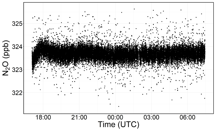
From the 15 h ambient air sampling in our closed laboratory, we observed that the water vapour concentration in the ambient air dropped from approximately 2500 ppm to about 800 ppm within the first 30 min. It continued to decrease progressively throughout the sampling period; however, after 5 h, the water vapour concentration somewhat stabilised, with a mean H₂O concentration of 476.9 ppm with a standard deviation of 18.7 ppm for the rest of the sampling. Note that these observed changes in water vapour might be partly due to the analyser's warm-up period. We therefore discarded the initial 5 h of data and used the remaining data to assess the signal stability and noise characteristics of the Aeris-N₂O. The Aeris-N₂O demonstrated a very stable signal with no apparent drift for about 10 h of sampling period, having a low standard deviation of 0.290 ppb. Using Allan deviation plots (Allan, 1987), we evaluated the analyser's noise characteristics and found that the Aeris-N₂O showed low instrument noise, approximately 0.18 ppb at 2 s averaging (see Fig. 3).

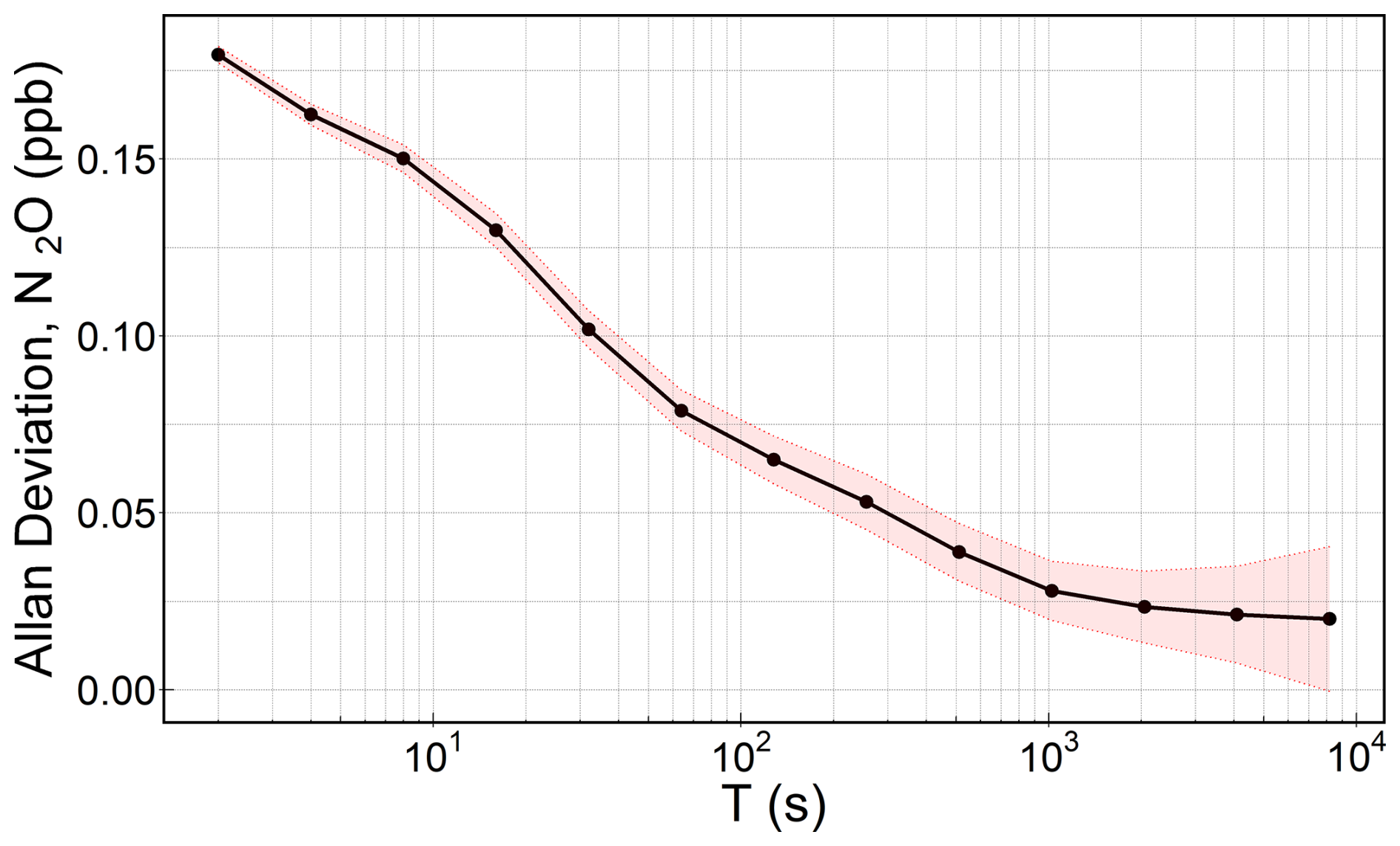
Figure 3 Computed Allan deviation plot based on 10 h of continuous sampling, following a 5 h spin-up period during which the water vapour mole fraction was not stable. Here, T is the sampling time in log-scale and the shaded region represents the 95 % confidence interval.

Because PGAs are known to be sensitive to fluctuations in water vapour concentration, we tested the Aeris-N₂O against different relative humidity (RH) conditions. Our tests with four RHs (approx. 28 %, 45 %, 60 %, and 83 %, respectively) showed that the water interference of the Aeris-N₂O was very small; we observed only slight differences in the mean N₂O concentrations for each humidity level (see Fig. 4), with mean N₂O concentrations of 332.7, 332.6, 332.7, and 332.5 ppb for RHs of 28 %, 45 %, 60 %, and 83 %, respectively. Furthermore, we observed the same standard deviation of about 0.3 ppb for each humidity level. Overall, our conducted laboratory tests indicated that the Aeris-N₂O was a suitable instrument for measuring low N₂O fluxes, showing low noise and water interference, along with negligible signal drift after the laser warms up. Nevertheless, the long warm-up period (approximately 5 h) of the analyser needs to be taken into account, as this can be a limiting factor for certain applications. To mitigate this, the Aeris-N₂O remained powered on throughout the whole field campaign.

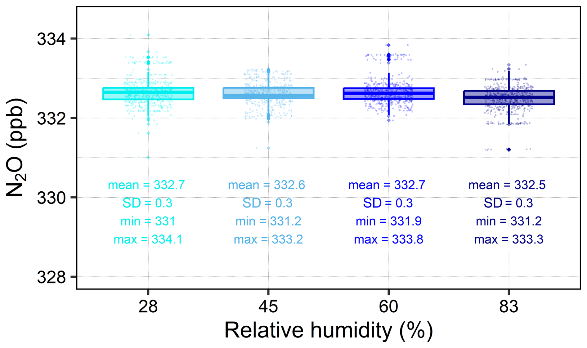
Figure 4 Measured N₂O concentrations for different relative humidities (RHs), with basic statistics of each RH summarised under each box plot. Each humidity level was sampled for approximately 20 min; however, only a 10 min window was used for further calculations. For our tests, we used a standard gas with a mean of 333.16±0.16 ppb as input. Jittered points are overlaid on the boxplots to visually separate overlapping data points, illustrating the distribution and density of the data.

3.2 Impact of chamber closure time on N₂O fluxes

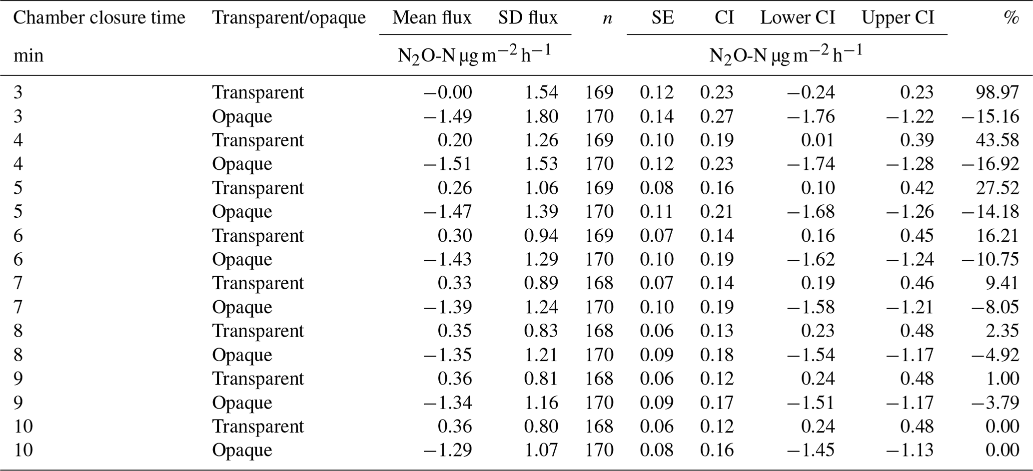
At our site, we commonly observed net N₂O consumption, suggesting an atmospheric sink, with a mean flux of −0.469 µg N₂O-N ${\mathrm{m}}^{-\mathrm{2}}{\mathrm{h}}^{-\mathrm{1}}$ and a 95 % confidence interval (CI) of ($-\mathrm{0.60},-\mathrm{0.3}$) during a chamber closure time of 10 min. Our calculated mean flux during transparent measurements was 0.361 µg N₂O-N ${\mathrm{m}}^{-\mathrm{2}}{\mathrm{h}}^{-\mathrm{1}}$, with a 95 % CI of (0.24,0.48) during a chamber closure time of 10 min (Table 1). For opaque measurements, our calculated flux was −1.29 µg N₂O-N ${\mathrm{m}}^{-\mathrm{2}}{\mathrm{h}}^{-\mathrm{1}}$, with a 95 % CI of ($-\mathrm{1.45},-\mathrm{1.13}$), indicating that our opaque measurements represent a real biochemical process, rather than an experimental artefact, in the (sub-) Arctic ecosystem. Nevertheless, the impact of environmental drivers on N₂O fluxes, including the transparent and opaque measurements, is beyond the scope of this study. Overall, we collected 338 samples, with 60 %–90 % of N₂O fluxes above the detectable limit. We therefore also acknowledge the possibility of unknown chamber artefacts that may remain undiscovered and could affect the interpretation of our data.

Table 1 Comparison of chamber closure times for both transparent and opaque measurements, with SE = standard error, CI = confidence interval, and % = percentage difference for the absolute mean flux of chamber closure time, compared with a chamber closure time of 10 min. CI is the margin of error calculated at 1.96×SE; the lower CI is calculated as mean flux − CI; the upper CI as mean flux + CI.

While chamber measurements are essential for understanding GHG emissions, they can alter soil–air conditions and introduce observational artefacts. These include potential impacts, such as pushing atmospheric air into the soil when closing the chamber, flushing soil gas into the chamber head space, and changing conditions during closure, e.g. increasing temperature and humidity inside the chamber due to soil and plant evaporation (Subke et al., 2021; Rochette and Eriksen-Hamel, 2008). As a result, the N₂O concentration gradient between the soil and the chamber head space and potentially also the functioning of plants and soil microbes are altered and may cause a bias in the flux estimates (Davidson et al., 2002). At our site, condensation within the chamber during a measurement period increased drastically with time, especially in the colder months. Although our laboratory tests showed that, for the Aeris-N₂O, increased water vapour does not interfere with N₂O concentrations, all laser cells are sensitive to water vapour. A too high water vapour content can, even with a filter assembly (1 µm pore size) within the tube, reach the analyser cell and lead to an abrupt end of a field campaign (Fiedler et al., 2022). It is, therefore, crucial to know how water vapour concentrations vary over time during chamber closure. At our study site, H₂O concentrations during transparent measurements increased, on average, from below 10 000 up to >16000 ppm, depending on the season. When we look at the rate of change over each minute, i.e. 0–1, 1–2, 2–3 min, etc., we can see that this rate of change drastically decreased within the first 2 min, and then exponentially decreased with increasing chamber closure time (Fig. S5). In other words, H₂O concentrations rose drastically in the first 2 min (>1300 ppm; data not shown), after which they levelled out until around 8 min, before they started increasing again (Fig. S5). For opaque measurements, the impact followed the same pattern, but was of much smaller magnitude (approx. 600 ppm rise within the first 2 min; data not shown). Because the increase in H₂O concentration did not directly affect N₂O concentrations in our study, and was further considered when calculating the fluxes with goFlux (Rheault et al., 2024), we did not introduce further measures.

When using transparent chambers, temperature control is an additional constraint (Rochette and Hutchinson, 2015). Ideally, the chamber temperature remains stable throughout the measurement period. However, in the field, especially during sunny conditions, this is challenging to achieve without active cooling, as the chamber's transparency creates a greenhouse effect (Rochette and Hutchinson, 2015). An increase in temperature can enhance microbial activity, leading to either N₂O production or N₂O consumption and potentially causing biased N₂O concentrations (Rochette and Eriksen-Hamel, 2008; Clough et al., 2020). In our study, chamber temperatures during transparent measurements changed similarly to H₂O concentrations, with the strongest decrease occurring within the first minutes of the measurement period (Figs. S5 and S6). At our site, temperature increased by around 0.7°C within the first 2 min, which slowed down to 0.3°C after 5 min (data not shown). During opaque measurements, temperature within the chamber decreased slightly by a maximum of 0.2°C in the first 2 min and below 0.1°C after 3 min (data not shown). It is likely that, during transparent measurements, the abrupt temperature increase in the first 2 min may have impacted N₂O concentrations (Parkin and Venterea, 2010). However, we refrained from using cooling systems, such as heat exchangers or ice packs, since they also have drawbacks, e.g. causing additional condensation within the chamber (Clough et al., 2020; Fiedler et al., 2022). As a result, we cannot exclude potential temperature effects from our N₂O concentration measurement during our measurement periods. Even though temperature changes are considered in the final flux calculation (Rheault et al., 2024), we argue that temperature changes inside chambers call for shorter closure times.

To minimise disturbances to the soil gas–atmosphere gradient and obtain flux estimates close to pre-deployment levels, several researchers have recommended using short chamber closure times of around 5 min (Fiedler et al., 2022; Pavelka et al., 2018; Venterea and Baker, 2008). This is because, during chamber closure, mean flux rates vary as N₂O builds up or decreases in the chamber head space (Rochette and Hutchinson, 2015). As closure time increases, the concentration gradient between the soil and the chamber head space decreases, reducing the diffusive flux. Within a closed system, gases can reach a temporary state of equilibrium over time, where the rate of N₂O production in the soil balances with the rate of N₂O release into the chamber head space (Fiedler et al., 2022). Our results suggest that, for transparent measurements, a chamber closure time of 3 min is too short and may result in significantly lower flux rates than longer chamber closure times (ANOVA, p<0.05 for 3 min, compared with 8, 9, and 10 min; Fig. 5). This discrepancy may be attributed to low microbial activity, or the possibility that N₂O production is countered by its rapid uptake or dissolution in the water present in the soil matrix, a phenomenon previously observed for CO₂ (Widén and Lindroth, 2003). From 4 min onward, our calculated mean N₂O flux rates are not significantly different from one another (Table 1). The proportion of transparent fluxes above the minimum detectable flux (MDF) increased from 62.7 % to 78.6 % as closure time increased from 3 to 10 min (Fig. 5a). While longer closure times reduce uncertainty and the amount of fluxes below the MDF, the gain is small after 4 min. We thus recommend chamber closure times of more than 4 min for reliable N₂O flux estimates, as this balances the need for accurate transparent measurements while minimising soil disturbance, as well as the impact of increasing temperature on N₂O concentrations within the chamber.

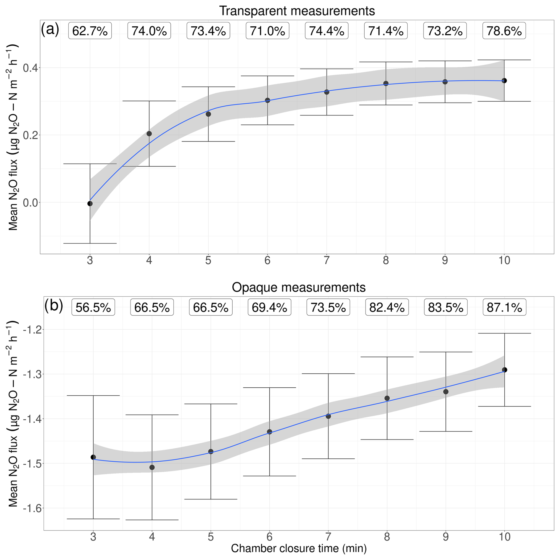
Figure 5 Mean N₂O fluxes (note: not concentrations) for transparent and opaque measurements, with number of measurement periods above the minimum detectable flux (MDF, %). Note the different y axes for the upper and lower plots. The range indicates the upper and lower limit of the 95 % confidence interval.

For opaque measurements, we find that our calculated fluxes show higher N₂O uptake from shorter chamber closure times, with flux rates around 15 % lower at 3–5 min than at 10 min, respectively (Table 1). At 6 min, the difference in our calculated N₂O uptake was still 10 % higher than at 10 min, decreasing to below 8 % between 7 and 9 min. At the same time, the MDF increased from 56.5 % to 87.1 % between 3 and 10 min (Fig. 5b). Nevertheless, none of the flux rates across different closure times was significantly different from any other (Kruskal–Wallis, p=0.99). Especially for N₂O uptake, it is essential to keep the chamber closure time as short as possible. This is because N₂O availability through soil diffusion is often the limiting factor for microbial consumption, i.e. atmospheric N₂O consumption by N₂O-reducing microbes (Liu et al., 2022). When the chamber is closed, the N₂O concentration in the head space decreases as N₂O diffuses into the soil, driven by the concentration gradient. As a result, the uptake rate also decreases, since N₂O reduction may become substrate-limited. Consequently, long chamber closure times may underestimate the uptake of atmospheric N₂O. Our analysis of the chamber closure time confirms this: during opaque measurement, we found that the uptake rate was greatest at 3–5 min and decreased with every minute of added chamber closure time (Fig. 5). For opaque measurements, we therefore suggest keeping the chamber closure time between 3 and 5 min, unless very few data points are available, when aiming for fluxes above the MDF becomes more important.

With the goFlux output, we obtain an individual MDF for each measurement period, allowing us to determine on a case-by-case basis if a flux is above the MDF. For both transparent and opaque measurements, the MDF in our study was, on average, $\mathrm{0.03}\mathrm{\mu }\mathrm{mol}{\mathrm{m}}^{-\mathrm{2}}{\mathrm{h}}^{-\mathrm{1}}$. This is lower than the MDF of $\mathrm{0.18}\mathrm{\mu }\mathrm{mol}{\mathrm{m}}^{-\mathrm{2}}{\mathrm{h}}^{-\mathrm{1}}$ reported in other nutrient-poor ecosystems by Christiansen et al. (2015) (Table 1). However, as mentioned previously, more than 40 % of the fluxes were below the MDF at 3 min closure time. This confirms that very short closure times can lead to higher uncertainties in flux estimates because the concentration changes are too small to be accurately detected (Fiedler et al., 2022). It is, therefore, essential to consider the precision of the instruments used in the field to identify the best-suited chamber closure time. With the Aeris-N₂O, we recommend chamber closure times above 4 min for transparent N₂O measurements in low-nutrient ecosystems. The optimal closure time depends on factors such as effective chamber height, micro habitat, and the duration of the field campaign. Shorter closure times allow for more repetitions, increasing the number of observation per chamber base position or adding more replicates, which are essential for the accurate representation of spatial variability (Jungkunst et al., 2018). For opaque measurements, we suggest shorter chamber closure times of 3–5 min. These findings are in line with other studies (Cowan et al., 2014; Kroon et al., 2008; Christiansen et al., 2015) but confirm, for the first time, that these recommendations are applicable to (very) nutrient-poor ecosystems.

3.3 Impact of linear and non-linear flux calculation approaches on N₂O fluxes

To facilitate understanding of how N₂O concentration build-up or reduction in the chamber head space can result in different flux estimates, goFlux automatically produces scatter plots with defined criteria (Fig. 6). These outputs allow for visual control of all measurement periods; additionally, csv outputs with the pre-defined quality checks are automatically produced. Our analysis using the goFlux package (Rheault et al., 2024) revealed that 59 % (n=2560) of all N₂O fluxes during different chamber closure times were best described by the HM model, indicating non-linear concentration changes over time. In contrast, 41 % (n=1728) of the fluxes were better explained by the LM model, showing a linear concentration change over time. However, all of the 41 % fluxes calculated with the LM model had no HM flux, meaning that the software did not calculate a non-linear flux because the HM model gave the same results as the LM model, and therefore favoured the LM model. In other words, all fluxes were either calculated using the HM model or resulted in the same values as the LM model. This finding has two possible reasons: the first is that the linearity might be an outcome of short measurement time and low flux, so that the non-linear model was reduced to a linear model; the second is an overestimation of the flux (Kutzbach et al., 2007). Linear and non-linear models for concentration data during chamber closure may typically be seen as alternatives, not complementary approaches. However, the non-linear fitting includes the linear fitting as a special case. When using a generic exponential function ae^−bt to fit data, where a and b are positive constants to be fitted, the function can be approximated to a linear function if the data points are distributed linearly. This is because the exponential function can be expanded as a series and, when the rate constant b is small, the linear function dominates. Namely, the first three terms of the serial expansion are $a(\mathrm{1}-bt+(bt{)}^{\mathrm{2}}/\mathrm{2})$, but when b is very small, i.e. b≪1, it is reduced to a(1−bt), which is the linear form. The slope of the linear term is −ab; if we take the time derivative of the original exponential function to calculate the slope, it gives $-ab{\mathrm{e}}^{-bt}$. When we expand it as a series and only take the first-order term as b≪1, we again obtain the simplified −ab as the slope. This means that, if the data points are linear, the exponential fitting will automatically reduce to a linear fitting with the same slope. With our results, we show that for N₂O fluxes, indeed, flux estimates were reduced to the linear model and yielded identical results to the non-linear model. The second reason for favouring linear models in goFlux is that an unexplained non-linearity can occur in the curvature, i.e. there may be non-exponential curvatures, which can result in an overestimation of the flux estimates (Kutzbach et al., 2007). In goFlux, the curvature of the non-linear model can be restricted with g_f (see Sect. 2.3). If the curvature was too large, leading to flux estimates over 4 times higher (with a g_f=4) than those from the linear model, the linear model was favoured. When we used a lower g_f of 1.25 for comparison, i.e. allowing HM fluxes to be at most 25 % higher than for the LM, we found that about one-quarter of the fluxes estimated by the non-linear model would have been excluded due to significant overestimation.

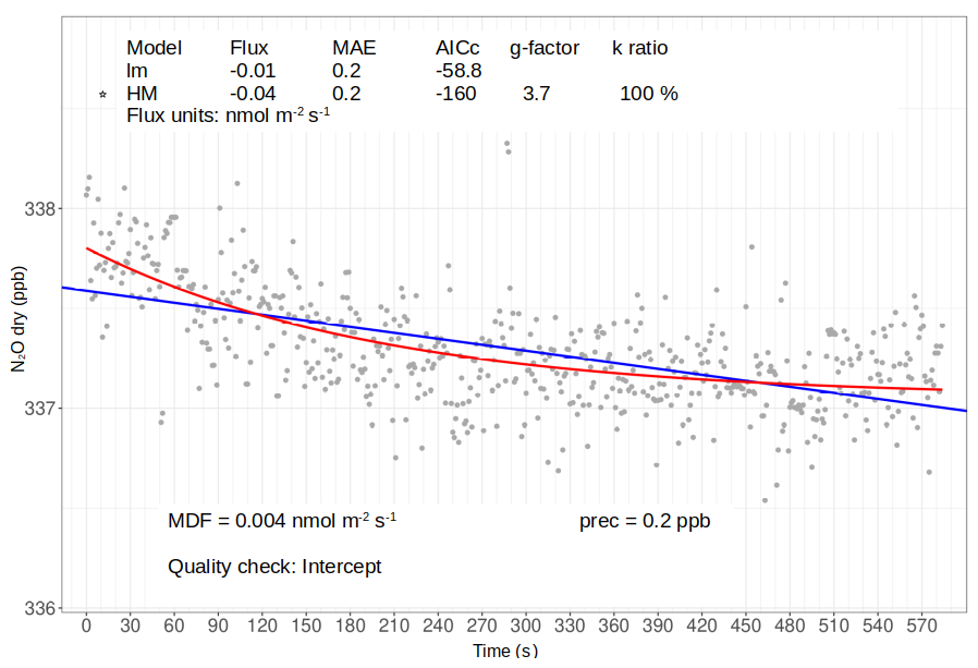
Figure 6 Example of scatterplot output from goFlux, showing N₂O concentrations in ppb from one measurement period, with information on linear (LM, blue line) and non-linear (HM, red line) flux calculations. For every measurement period, the chosen model is marked with a star (here, HM) according to the pre-defined quality check, indicated on the bottom of the graph (here, intercept). Flux values, mean absolute error (MAE), Akaike information criterion corrected (AICc) for model performance, g factor, and k ratio are shown on top of the figure; here, a g factor of 3.7 indicates that the HM flux value is 3.7 times higher than the one obtained from LM. Source: goFlux package (Rheault et al., 2024), font sizes modified.

There is a tendency to favour LM over HM models in the literature, primarily due to their simplicity. It is also generally assumed that concentration changes are linear during short chamber closure times, keeping uncertainties low (Hüppi et al., 2018; Kroon et al., 2008). However, because GHG concentrations naturally follow a non-linear behaviour within a closed system due to diffusion theory (Fick's first law) and leakage (Anthony et al., 1995; Kroon et al., 2008), LM models may introduce a bias, differing from HM model estimates by up to 60 % (Hüppi et al., 2018; Kroon et al., 2008), resulting in less accurate flux estimates and GHG budgets. This has been thoroughly investigated for N₂O fluxes by Kroon et al. (2008), who found a large underestimation of N₂O fluxes by the LM model in their study. With our results, we suggest that all future N₂O flux chamber calculations should be made using HM models, which can be filtered for overestimation of fluxes when flux rates are larger. Novel software packages, such as goFlux (Rheault et al., 2024), offer the possibility to easily integrate both LM and HM models and report the flux rates in a reproducible way. We believe that these approaches will be crucial to facilitate the use of both LM and HM models and, as a consequence, enable the chamber community to standardise their flux calculation methods. We further emphasise the importance of using all available data points for flux estimates, rather than selecting a subset of linear data. This is because our approach, which involves filtering out unrealistic values and visually verifying measurement periods after flux calculation, enhances the reproducibility and consistency of N₂O flux estimates.

3.4 Simulated differences in N₂O flux rates between GC and PGA

Our results indicate that, for transparent measurements, the N₂O fluxes we calculated using three simulated GC samples were, on average, 21.7 % lower than the PGA fluxes (0.085 µg N₂O-N ${\mathrm{m}}^{-\mathrm{2}}{\mathrm{h}}^{-\mathrm{1}}$; data not shown). Specifically, positive values, i.e. efflux, were generally underestimated (p<0.001, $R_{\text{adj}}^{\mathrm{2}}=\mathrm{0.37}$, Fig. 7). When we calculated fluxes using four simulated GC samples, negative N₂O fluxes appeared to be nearly identical to the N₂O uptake we calculated from the PGA (600 data points); however, efflux was still underestimated by 3 % (p<0.001, $R_{\text{adj}}^{\mathrm{2}}=\mathrm{0.65}$). Interestingly, by increasing the number of samples to five or six, our calculated fluxes seemed to underestimate N₂O uptake, whilst efflux was overestimated (p<0.001, $R_{\text{adj}}^{\mathrm{2}}=\mathrm{0.85}$, Fig. 7). Overall, the N₂O fluxes we calculated using five samples underestimated N₂O fluxes by 2.2 %, while calculations with six samples resulted in an overestimate of around 2.4 % (data not shown).

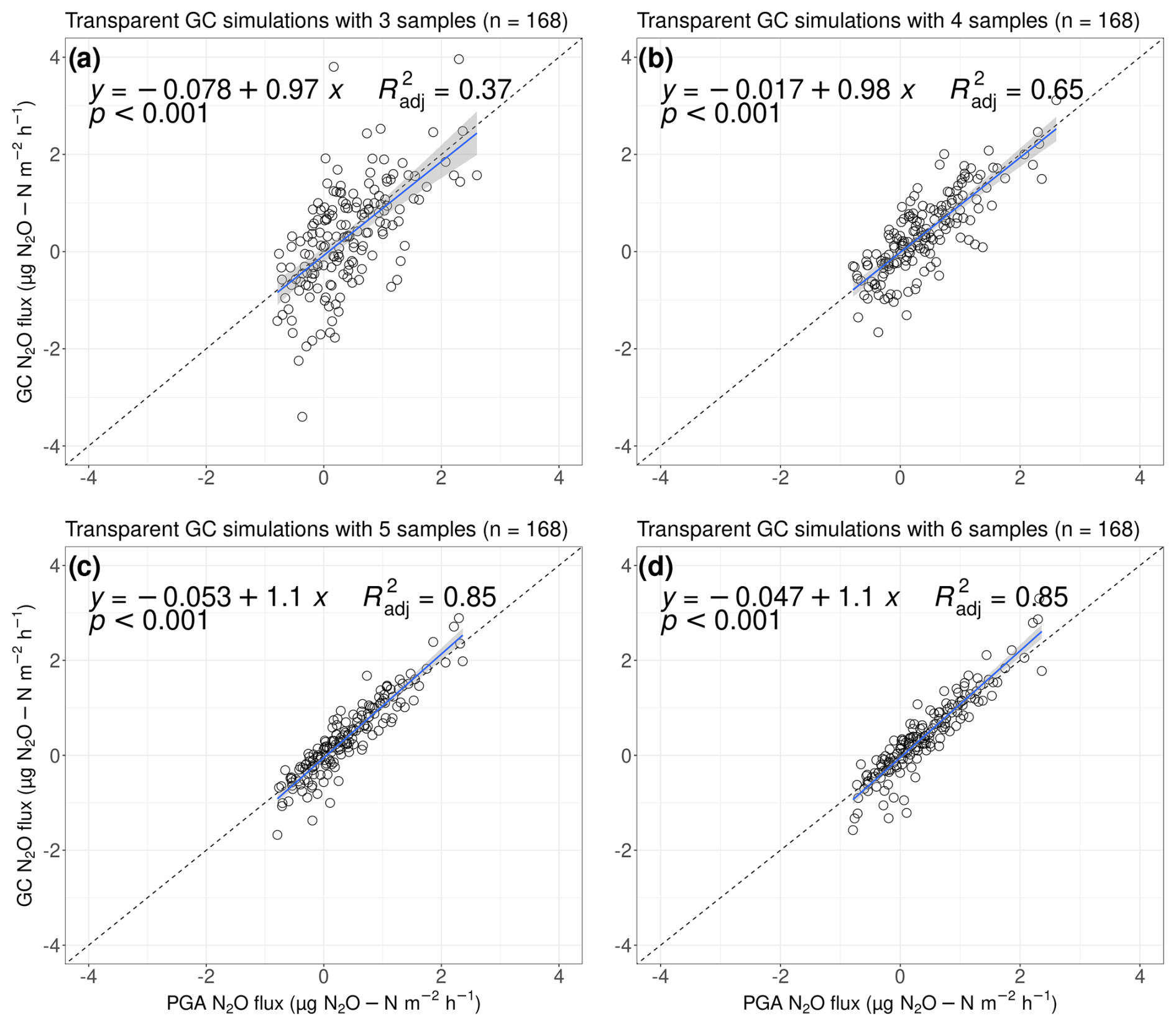
Figure 7 Simulated GC fluxes from light measurements with (a) three, (b) four, (c) five, and (d) six samples compared with flux measurements taken with our PGA for 10 min (n=168). All fluxes were calculated with the goFlux package; results from “best.Flux” are shown. The blue trend line fits a generalised linear model, with the shaded area representing the 95 % confidence interval. The shown equations and $R_{\text{adj}}^{\mathrm{2}}$ values follow the y∼x equation.

For opaque measurements, all N₂O flux estimates we calculated from GC simulations were lower than the flux estimates we calculated from the PGA, with underestimates of 6.6 %, 2.3 %, 7.9 %, and 8.1 % for three, four, five, and six sample points, respectively (data not shown). With three samples, the calculated uptake rates were generally overestimated, while efflux was underestimated. When we calculated fluxes using four simulated GC samples, N₂O uptake was still overestimated, while with five and six sample points it was slightly underestimated. However, compared with transparent measurements, the values of $R_{\text{adj}}^{\mathrm{2}}$ were low (Fig. 8, $R_{\text{adj}}^{\mathrm{2}}=\mathrm{0.21}$, 0.51, 0.69, and 0.68, respectively). The underestimation of GC fluxes may occur as a result of a smoothed-out curve: when only a few data points are available, variations in curves are naturally reduced. Furthermore, the precision of our GC was 1.9 ppb, compared with 0.2 ppb of the Aeris-N₂O, resulting in less accurate measurement of the N₂O concentrations. This may lead to a loss of detail in the curve, particularly in the peak values of the N₂O concentrations, which can result in underestimation of the flux.

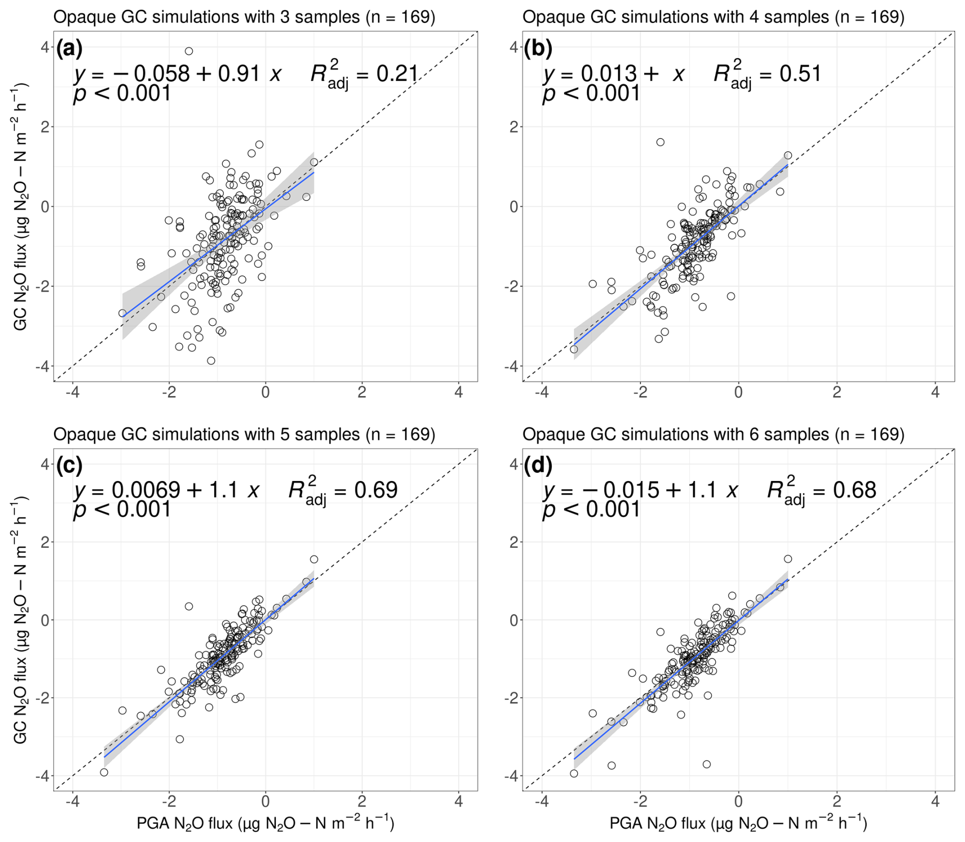
Figure 8 Simulated GC fluxes from opaque measurements with (a) three, (b) four, (c) five, and (d) six samples, compared with flux measurements taken with our PGA for 10 min (n=338). All fluxes were calculated with the goFlux package; results from “best.Flux” are shown. The blue trend line fits a generalised linear model, with the shaded area representing the 95 % confidence interval. The shown equations and $R_{\text{adj}}^{\mathrm{2}}$ values follow the y∼x equation.

It is important to note that our comparison was made between our PGA and simulated GC measurements (Fig. 9). For the GC simulations, we adjusted the instrument precision during the flux calculation, but no actual air samples were analysed by any GC instrument. Furthermore, our chamber closure time was considerably shorter than for most GC studies because of the condensation and temperature changes within the chamber. During prolonged chamber closure times, significant changes in the concentration gradient and chamber conditions can take place (see previous discussion), which are unlikely to be replicated in our GC simulation. This difference in experimental design may actually be beneficial, as it allows us to isolate and study the effects of shorter closure times on N₂O flux measurements. Furthermore, our sensitivity analysis with four simulated GC samples showed that, even when we changed the sample times by ±60 s compared with the original time stamp, flux rates differed less than 10 %, with $R_{\text{adj}}^{\mathrm{2}}$ values between 92 and 98 (data not shown). We believe that the underestimation of N₂O flux rates we calculated is, therefore, not a result of an inadequate simulation but needs to be verified by future studies actually measuring N₂O samples from nutrient-poor ecosystems in a GC.

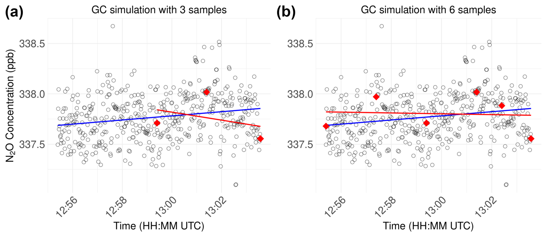
Figure 9 Examples visualising the comparison of regression slopes obtained using 600 data points from the portable gas analyser (blue line) vs. (a) three or (b) six virtual samples, mimicking manually defined sample times for subsequent analysis in a gas chromatograph (red line).

Our results are consistent with previous studies that compared N₂O flux rates between GCs and PGAs (Fig. 9), which concluded that GCs were suitable for measuring N₂O fluxes under certain conditions (Christiansen et al., 2015; Brümmer et al., 2017). Christiansen et al. (2015) investigated the differences between a fast-responding analyser (a cavity ring-down spectroscopy analyser; Fleck et al., 2013) and a high-precision GC in agricultural fields in Vancouver, Canada, by taking five GC samples at chamber closure times of 0, 3, 10, 20, and 30 min. They found that N₂O fluxes were very similar and did not differ significantly, with average N₂O fluxes of 47.6±8.4 µg N₂O-N ${\mathrm{m}}^{-\mathrm{2}}{\mathrm{h}}^{-\mathrm{1}}$ from the fast-responding analyser and 61.6±11.2 µg N₂O-N ${\mathrm{m}}^{-\mathrm{2}}{\mathrm{h}}^{-\mathrm{1}}$ from GC. With a similar setup, Brümmer et al. (2017) compared N₂O fluxes measured by a fast-responding analyser similar to the Aeris-N₂O (a quantum cascade laser) and a GC from a low-flux agricultural grassland in Braunschweig, Germany. Their four GC samples, taken at 0, 20, 40, and 60 min, were highly scattered and rarely showed a distinctive trend, introducing a wide range of N₂O fluxes between −26 and 39 µg N₂O-N ${\mathrm{m}}^{-\mathrm{2}}{\mathrm{h}}^{-\mathrm{1}}$, with a standard error between 1 and 44 µg N₂O-N ${\mathrm{m}}^{-\mathrm{2}}{\mathrm{h}}^{-\mathrm{1}}$. In contrast, the N₂O fluxes measured by the fast-responding analyser only varied between 4 and 32 µg N₂O-N ${\mathrm{m}}^{-\mathrm{2}}{\mathrm{h}}^{-\mathrm{1}}$, with standard errors below 1.2 µg N₂O-N ${\mathrm{m}}^{-\mathrm{2}}{\mathrm{h}}^{-\mathrm{1}}$. This highlights three critical aspects: first, despite claiming low-flux environments, flux rates from agricultural fields are much higher than from a sub-Arctic peatland or other nutrient-poor ecosystems (Savage et al., 2014; Cowan et al., 2014), where capturing N₂O fluxes is even more challenging. Second, low N₂O fluxes tend to be widely scattered, with a lot of noise in comparison with the actual trend, i.e. the change in concentration during chamber closure. This makes it very challenging to find trends when calculating fluxes if only a few samples are available, let alone to show N₂O uptake without high uncertainties (Cowan et al., 2014). Finally, it is crucial to know and test the precision of the instruments used in the field to get reliable flux estimates and minimum detectable fluxes (Kutzbach et al., 2007; Christiansen et al., 2015).

Our findings suggest that calculating N₂O fluxes from three GC samples is likely to lead to an underestimation of the “real” flux (Kutzbach et al., 2007). We therefore strongly advise against using only three samples, as flux calculations may have to be discarded if only one sample is erroneous. In contrast, using four to six samples yields very comparable results to those obtained with a PGA, depending on the precision of the GC method. However, the small sample size restricts our ability to confidently identify trends in N₂O fluxes. Undetected errors can bias flux estimates due to the high impact of each data point on the regression slope. To compare previous N₂O flux measurements with novel data sets measured with a PGA, it is crucial to investigate differences between these methods. To achieve this, novel instruments have to be tested for their precision, noise, and accuracy, as well as potential interference with water vapour (Grace et al., 2020; Ahmed et al., 2024).

We suggest that measuring N₂O fluxes with fast-responding analysers in nutrient-poor ecosystems should be considered for all future studies. PGAs, for example, have two main advantages over the GC method: they collect a large amount of sample points, and the quality of these can be checked in situ during the measurement period. With more samples, there are more data points; this then results in the option to reduce chamber closure times and further reduce artefacts caused by sealing off a part of a soil profile in a closed chamber (Brümmer et al., 2017). If errors happen in the field, e.g. leakage and pressure change (Rochette and Hutchinson, 2015), they are visible in the online interface of the PGA. This real-time in situ control of N₂O concentrations allows for direct optimisation in the field and increases the quality of flux measurements (Fiedler et al., 2022). A practical result of that is that measurement periods can be interrupted and repeated in the field at any time, ensuring high quality of the flux measurements, as well as an optimal use of time in the field, particularly since chamber closure times with PGAs are shorter than with GCs. However, PGAs have some drawbacks: weighing 10–20 kg (including batteries), they are heavier than GC vials. Additionally, their power consumption requires regular backups, and heavy vibrations, particles, water, and sudden pressure changes can contaminate the laser cell (Fiedler et al., 2022). With good planning and care, it is, however, easily possible to deal with these disadvantages.

4 Conclusions

In our study, we established a manual flux chamber method using a portable gas analyser (PGA) capable of quantifying low N₂O fluxes in nutrient-poor ecosystems and, based on our extensive experience with the system, provide detailed practical suggestions on how to collect high-quality measurements in low-flux ecosystems (see the Supplement). To our knowledge, our study represents the first extensive analysis of N₂O fluxes measured with manual flux chambers in a (very) nutrient-poor, (sub-) Arctic ecosystem. Our laboratory tests confirmed that our PGA (Aeris MIRA Ultra ${\mathrm{N}}_{\mathrm{2}}\mathrm{O}/{\mathrm{CO}}_{\mathrm{2}}$) is well suited for measuring low N₂O fluxes, with low noise, minimal water interference, and negligible signal drift. With our PGA–chamber system, we are able to report very low N₂O flux values with positive and negative signs, indicating both N₂O efflux and uptake. Because PGAs allow for near-continuous monitoring of concentration changes with high precision and low detection limits, we recommend, with a chamber height of 25 cm, chamber closure times of 3–5 min for opaque and >4 min for transparent measurements to minimise the impacts of the ecosystem due to the measurement setup (e.g. changes in temperature and humidity). To strike a balance between detection sensitivity and measurement efficiency, we suggest using a standard 5 min closure time for all measurements, with smaller chambers, which enables us to detect around 70 % of fluxes. This allows for most N₂O fluxes to be detected in this setup; however, the sensitivity depends on the effective chamber height.

We further recommend using non-linear models for N₂O flux calculations (HM; Hutchinson and Mosier, 1981) with filters to address overestimation at higher flux rates. Novel software packages, such as goFlux (Rheault et al., 2024), simplify the integration of both linear and non-linear models, and report flux rates in a reproducible way; such approaches are key to standardising flux calculations across the chamber community. Using non-linear models, as well as standardised and well-documented calculation and quality control, allows consideration of the entire time series of measurement periods, and does not require (subjective) expert knowledge to first restrict the datasets to a suitable section and only afterwards calculate flux estimates. We stress this importance of using all available data points for flux estimates to improve the reproducibility and consistency of N₂O flux estimates.

We recommend using PGAs in future N₂O studies in nutrient-poor ecosystems whenever feasible. PGAs collect more data points (typically about 1 sample s⁻¹) and allow for real-time quality control in the field, while GC measurements may be limited by low flux rates and thus fall below the detection limits or lack clear trends. To get the most out of PGAs, it is essential to determine their precision and use a suitable chamber closure time. In that way, most N₂O fluxes can be detected; this is especially important in nutrient-poor ecosystems, where N₂O fluxes are often very low. Future studies using other chamber designs may benefit from re-evaluations of chamber closure times and flux calculation methods to find optimum customised setups.

While this study concentrates on the methodological aspects of quantifying N₂O fluxes in a nutrient-poor ecosystem, a follow-up study will investigate the environmental drivers of N₂O fluxes. Because most studies in the (sub-) Arctic have reported N₂O from opaque measurements only, there is a lack of data on how soil N₂O fluxes differ in various light conditions, especially in Arctic ecosystems (Stewart et al., 2012). Our results demonstrate notable differences between transparent and opaque conditions that require further investigation. This fills an important gap in N₂O studies from the Arctic, where negative fluxes have been observed but could not be investigated due to measurement accuracy not being high enough (Voigt et al., 2020). Further, this novel finding highlights the need for future research on N₂O fluxes in sub-Arctic ecosystems and other nutrient-poor ecosystems, and their potential response to global warming.

Appendix A

Ambient air was sampled using an Aeris-N₂O analyser; Fig. A1 shows the entire 15 h long run without removing the first 5 h (1 Hz), where the water vapour mole fractions were not stable.

Figure A1 Time series of N₂O analyser for 15 h long run.

Changes of H₂O mole fractions during the water interference test were investigated (see Fig. A2). Corresponding relative humidities were noted and the data used for the comparison are denoted with red vertical lines.

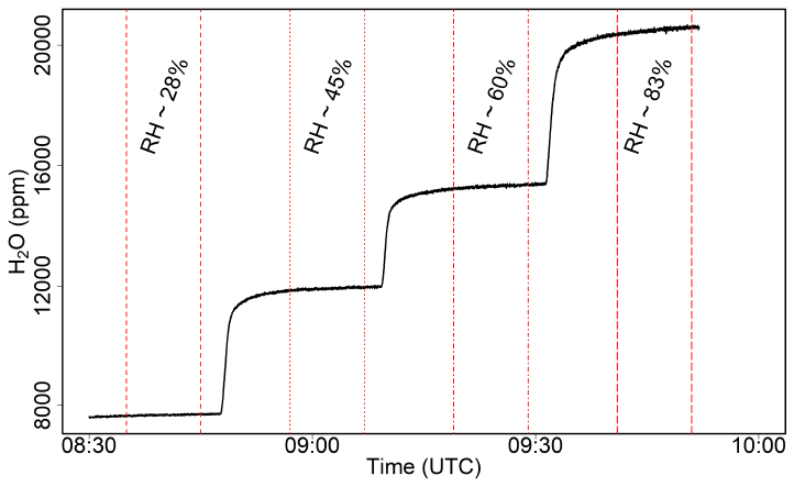
Figure A2 H₂O mole fractions measured by Aeris-N₂O analyser during the water interference test. The corresponding relative humidities (RHs) are given for each step. Red lines demonstrate the data used to assess the water interference at each RH step.