Best estimate of the planetary boundary layer height from multiple remote sensing measurements

Remote sensing measurements have been widely used to estimate the planetary boundary layer height (PBLHT). Each remote sensing approach offers unique strengths and faces different limitations. In this study, we use machine learning (ML) methods to produce a best-estimate PBLHT (PBLHT-BE-ML) by integrating four PBLHT estimates derived from remote sensing measurements at the Department of Energy (DOE) Atmospheric Radiation Measurement (ARM) Southern Great Plains (SGP) observatory. Three ML models – random forest (RF) classifier, RF regressor, and light gradient-boosting machine (LightGBM) – were trained on a dataset from 2017 to 2023 that included radiosonde, various remote sensing PBLHT estimates, and atmospheric meteorological conditions. Evaluations indicated that PBLHT-BE-ML from all three models improved alignment with the PBLHT derived from radiosonde data (PBLHT-SONDE), with LightGBM demonstrating the highest accuracy under both stable and unstable boundary layer conditions. Feature analysis revealed that the most influential input features at the SGP site were the PBLHT estimates derived from (a) potential temperature profiles retrieved using Raman lidar (RL) and atmospheric emitted radiance interferometer (AERI) measurements (PBLHT-THERMO), (b) vertical velocity variance profiles from Doppler lidar (PBLHT-DL), and (c) aerosol backscatter profiles from micropulse lidar (PBLHT-MPL). The trained models were then used to predict PBLHT-BE-ML at a temporal resolution of 10 min, effectively capturing the diurnal evolution of PBLHT and its significant seasonal variations, with the largest diurnal variation observed over summer at the SGP site. We applied these trained models to data from the ARM Eastern Pacific Cloud Aerosol Precipitation Experiment (EPCAPE) field campaign (EPC), where the PBLHT-BE-ML, particularly with the LightGBM model, demonstrated improved accuracy against PBLHT-SONDE. Analyses of model performance at both the SGP and EPC sites suggest that expanding the training dataset to include various surface types, such as ocean and ice-covered areas, could further enhance ML model performance for PBLHT estimation across varied geographic regions.

1 Introduction

The planetary boundary layer (PBL) refers to the lowest part of the Earth's atmosphere that directly interacts with the Earth's surface (Stull, 1988). This layer responds to surface forcing within 1 h or less and closely follows the diurnal cycle of surface heating and cooling over land (Deardorff, 1974; Xi et al., 2022). Within the PBL, turbulent motion drives significant exchanges of heat, mass, moisture, and momentum between the surface and the free troposphere. These exchanges significantly influence atmospheric processes, including aerosol mixing and transport, cloud formation and evolution, aerosol–cloud interactions (Painemal et al., 2017; Su et al., 2024), and precipitation formation, which strongly affect human activities (Teixeira et al., 2025). The vertical depth of PBL is represented by the planetary boundary layer height (PBLHT), which corresponds to an important parameter in atmospheric process studies and numerical model simulations (Zhang et al., 2020). The PBLHT is often used to characterize PBL structures and is a key factor for estimating flux exchanges between the surface and the atmosphere. Although there are several well-accepted definitions of the PBL, as described by LeMone et al. (2019), accurate estimates of the PBLHT remain challenging.

Due to the convective nature of the PBL, vertical gradients of thermodynamic parameters, including temperature (or potential temperature) and water vapor (or relative humidity) as well as trace gases and aerosols, are commonly used to estimate the PBLHT. For a well-mixed convective PBL, the PBL top is characterized by a positive gradient of potential temperature and negative gradients of water vapor, trace gases, and aerosols. Radiosonde data, offering high vertical-resolution measurements of temperature and moisture profiles, are widely used for estimating PBLHT (Liu and Liang, 2010; Seidel et al., 2010). However, radiosonde data suffer from poor temporal resolutions. Most radiosonde stations launch a sounding system only twice daily, making it challenging to study and understand the temporal evolution of the PBL based on radiosonde data. Model forecasts and reanalysis data have also been used to estimate global PBLHT climatology (von Engeln and Teixeira, 2013). However, the uncertainty and coarse spatiotemporal resolution of these data could prevent reliable estimates of PBLHT.

The use of continuous remote sensing observations provides a high temporal resolution of PBLHT estimates. These observations include sodar (Contini et al., 2008), radar wind profilers (Salmun et al., 2023), aerosol lidars (Dang et al., 2019; Su et al., 2020), Doppler lidar (DL) (Tucker et al., 2009; Krishnamurthy et al., 2021), water vapor and/or temperature lidars, and radiometers (Turner et al., 2014), as well as global navigation satellite system radio occultation (GNSS-RO) (Nelson et al., 2021). Although obtaining the vertical distribution of turbulence parameters remains challenging, these observations provide valuable data on the thermodynamic properties (e.g., water vapor and/or temperature lidars and radiometers), dynamic properties (e.g., sodar, radar wind profilers, DL, GNSS-RO), and the distribution of tracer substances (e.g., aerosol lidars) of the PBL, all of which can be used to estimate PBLHT. Kotthaus et al. (2023) present a comprehensive review of the capabilities and limitations of PBLHT estimates from ground-based remote sensing observations. When remote sensing instruments are deployed on various platforms, such as ground stations, aircraft, or spaceborne satellites, they can provide PBLHT estimates for fixed locations as well as on regional and global scales (Kalmus et al., 2022; Luo et al., 2016; Roldán-Henao et al., 2024a, b; Salmun et al., 2023; Scarino et al., 2014; Su et al., 2020; Xu et al., 2024).

It is important to note that different observational techniques capture varying characteristics of the PBL, and as a result, PBLHT estimates from different observations may differ significantly. Each observation has its own advantages and limitations. Radiosonde data offer high accuracy and high-vertical-resolution in situ measurements of atmospheric temperature and water vapor profiles, making PBLHT estimates from radiosondes more reliable than those from remote sensing observations. For example, the Vaisala RS92 radiosonde thermodynamic sensor can measure pressure, temperature, and relative humidity with accuracies of 0.5 hPa, 0.2 °C, and 2 %, respectively (Holdridge, 2020). As a result, radiosonde data are often used to evaluate PBLHT estimates from remote sensing methods (Su et al., 2020) or serve as the “ground truth” for training machine learning models (Krishnamurthy et al., 2021). Aerosol lidars and ceilometers (CEIL) use aerosol as a tracer for PBL observations (Zhang et al., 2022). These instruments are affordable, portable, and reliable even under harsh weather conditions. However, PBLHT estimates from aerosol lidars suffer from the impacts of the aerosol residual layer during nighttime and early morning, and from transported aerosol layers. DL directly employs the measured vertical velocity variance profile to estimate PBLHT. Studies show that the PBLHT estimated from DL compares well with that from radiosonde data, especially during the growing and decaying periods of the PBL evolution (Tucker et al., 2009). However, the DL approach is sensitive to the choice of velocity variance threshold and can vary as a function of the site. In addition, the approach has difficulty providing reliable PBLHT estimates under stable PBL conditions (Krishnamurthy et al., 2021). PBLHT estimates from thermodynamic profiles retrieved using water vapor/temperature lidars or high-spectral-radiometer measurements can employ the same methods as PBLHT estimates from radiosonde data, which work under a clear sky. However, the retrieved thermodynamic profiles sometimes suffer from significant retrieval uncertainties, which hinder the accurate estimate of PBLHT. Although no single method or measurement consistently provides the most reliable PBLHT estimates across all PBL schemes and environmental conditions, combining PBLHT estimates from multiple remote sensing techniques can lead to more accurate estimates under various conditions (Kotthaus et al., 2023).

Machine learning (ML) approaches offer powerful tools for integrating information from various observations, identifying patterns, making predictions, and gaining deeper insights from complex datasets. Even when the relationships between variables are not fully understood, ML methods enable the extraction of valuable knowledge from diverse data sources. ML techniques have been applied to improve PBLHT estimates. For example, Krishnamurthy et al. (2021) used a random forest (RF) model to enhance PBLHT estimates from DL measurements by combining PBLHT estimates from the Tucker method with environmental factors such as surface sensible and latent heat fluxes, wind speed and direction, surface upward longwave and shortwave radiation, soil moisture and temperature, the Monin–Obukhov length, and the cloud base height. Their results demonstrated significant improvements in PBLHT estimates compared to those derived solely from the Tucker method, validated against radiosonde data. Su and Zhang (2024) introduced a deep-learning framework trained on extensive remote sensing and radiosonde data, leveraging conventional meteorological measurements to produce robust and reliable PBLHT estimates across diverse environmental conditions. Several studies exploring various ML models, such as gradient-boosting regression trees, K-means clustering, AdaBoost, and deep neural networks, have shown enhanced PBLHT estimates from various remote sensing measurements (Rieutord et al., 2021; de Arruda Moreira et al., 2022; Liu et al., 2022).

In this study, we apply ML methods to enhance PBLHT estimates by integrating multiple remote-sensing-derived PBLHTs. Specifically, we utilize data from the micropulse lidar (PBLHT-MPL), ceilometer (PBLHT-CEIL), and Doppler lidar (PBLHT-DL) and thermodynamic profiles retrieved using Raman lidar (RL) and atmospheric emitted radiance interferometer (AERI) measurements (PBLHT-THERMO). We hypothesize that PBLHTs derived from observations of various PBL characteristics, e.g., thermodynamic effects (PBLHT-THERMO), dynamic effects (PBLHT-DL), and tracer particles (PBLHT-MPL and PBLHT-CEIL), complement each other. Together, they can provide valuable information on improving PBLHT estimates under various PBL schemes and environmental conditions. We use radiosonde-derived PBLHT (PBLHT-SONDE, more details in Sect. 2.2) to train ML models, aiming to predict the best estimate of PBLHT (PBLHT-BE) by combining the four approaches with ancillary environmental data. We use multiple years of advanced remote sensing and radiosonde data collected at the Department of Energy (DOE) Atmospheric Radiation Measurement (ARM) Southern Great Plains (SGP) atmospheric observatory to train ML models and test their predictions. In addition, we use remote sensing and radiosonde data from a recent ARM field campaign to test whether the ML method works at different locations.

The paper is organized as follows: Sect. 2 presents an overview of the ARM SGP site, its instruments and observations, PBLHT estimation approaches from radiosonde data, and various remote sensing observations. The ML method, training and testing, and feature importance analysis are presented in Sect. 3; finally, Sect. 4 presents the summary and conclusions.

2 ARM observation and PBLHT estimates

2.1 The ARM SGP site observations

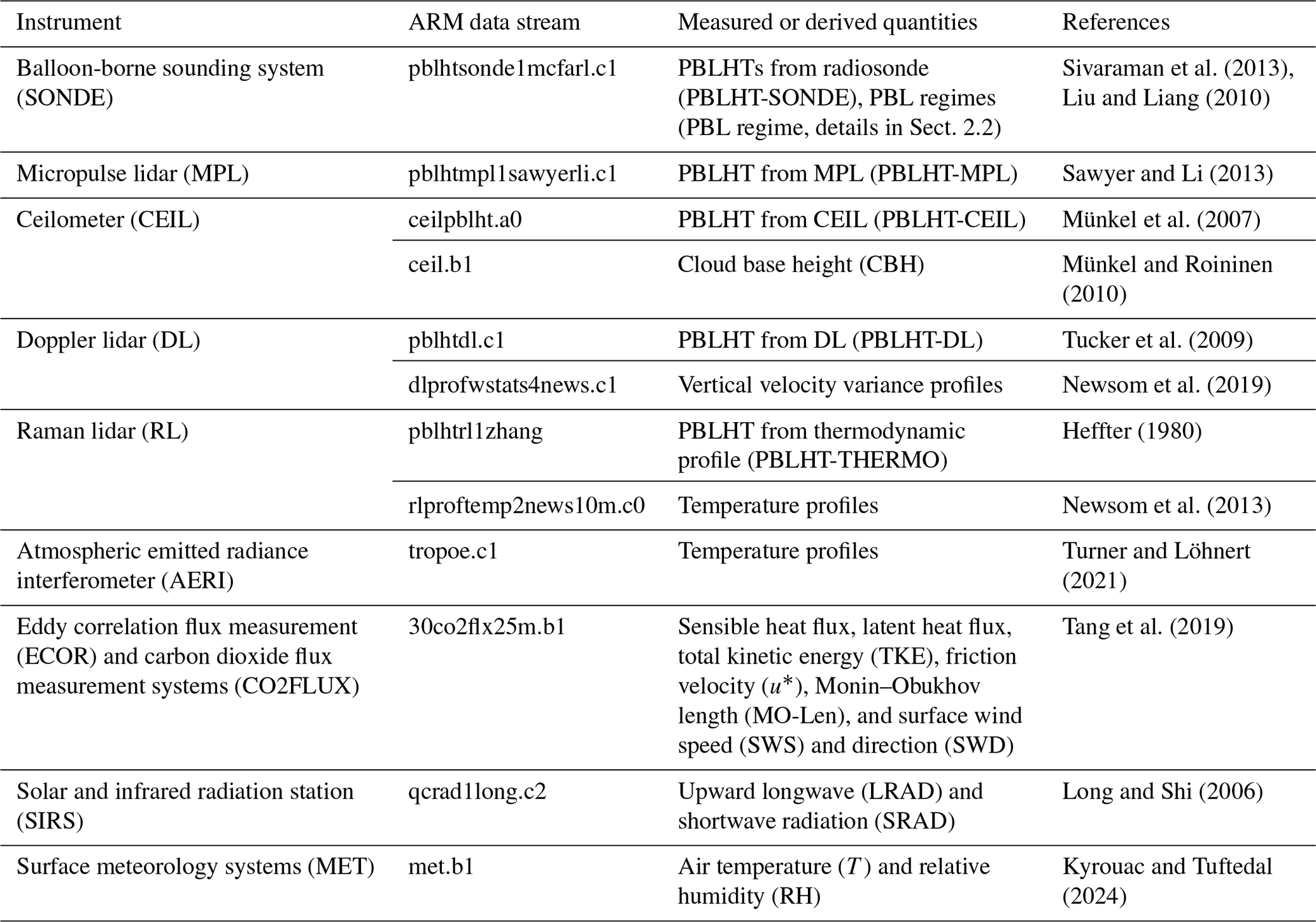
The DOE ARM user facility deploys advanced remote sensing and in situ instruments at climatically critical locations. The SGP atmospheric observatory central facility, located in north–central Oklahoma (36°36^′′26^′′ N, 97°29^′15^′′ W), is the world's most extensive ground-based climate research facility. Surrounded by cattle pasture and wheat fields, the SGP central facility is equipped with a wide range of advanced instrument clusters, providing critical observations for research on atmospheric-process-level studies of aerosol, clouds, precipitation, land–atmospheric interactions, etc. The advanced instruments include various radars, lidars, radiometers, aerosol/gas sampling instruments, and cloud sample instruments. A detailed description of these instruments can be found on ARM's SGP instrument web page (https://www.arm.gov/capabilities/observatories/sgp, last access: 21 September 2024) and in Mather and Voyles (2013). Key ground-based instruments, data streams, and the measurements used for PBLHT estimates are listed in Table 1. The SGP has been collecting data since 1992 and has accumulated extensive long-term datasets. This study utilizes the data collected between 2017 and 2023 for PBLHT analysis, as well as training and testing ML models.

Table 1 Key ground-based instruments and measurements at the SGP site used for PBLHT estimates.

2.2 PBLHT-SONDE value added product

The balloon-borne sounding system (SONDE) is typically launched four times a day at approximately 05:30 (00:30), 11:30 (06:30), 17:30 (12:30), and 23:30 UTC (18:30 LT), where the times indicate Universal Time Coordinate and the times in parentheses are in local time, at the SGP site. During intensive-observing periods (IOPs), SONDE launches occur more frequently, often up to eight times per day. SONDE measures vertical profiles of the atmospheric thermodynamic state, including atmospheric pressure, temperature, moisture, and wind speed and direction, with a temporal resolution of 1 s. This corresponds to vertical resolutions ranging from several meters to over 10 m. The measured temperature can reach an accuracy of 0.2 °C.

To estimate PBLHT, the ARM PBLHT-SONDE value-added product (VAP) applies three commonly used methods: the Heffter (1980), Liu and Liang (2010), and bulk Richardson number approaches (Seibert et al., 2000). Details of the three methods are described in the corresponding references and in Sivaraman et al. (2013). In brief, the Heffter method (PBLHT-Heffter) determines PBLHT as the lowest height where the potential temperature difference between a given height and the bottom of an inversion layer first reaches 2 K.

The Liu–Liang method (PBLHT-Liuliang) first classifies the PBL into three regimes: the convective boundary layer (CBL), stable boundary layer (SBL), and neutral residual layer (NRL). This classification is based on the potential temperature (θ) difference between the fifth and second levels of sounding data (θ₅−θ₂) compared to a stability threshold. CBL is identified when ${\mathit{\theta }}_{\mathrm{5}}-{\mathit{\theta }}_{\mathrm{2}}<-{\mathit{\delta }}_s$, SBL when ${\mathit{\theta }}_{\mathrm{5}}-{\mathit{\theta }}_{\mathrm{2}}>+{\mathit{\delta }}_s$, and NRL when $-{\mathit{\delta }}_s\le {\mathit{\theta }}_{\mathrm{5}}-{\mathit{\theta }}_{\mathrm{2}}\le +{\mathit{\delta }}_s$, where δ_s is the minimum strength of the inversion layer. The PBL scheme is a critical factor, as PBLHT estimates exhibit significantly different characteristics across different PBL regimes. As noted by Zhang et al. (2022), the CBL and NRL regimes can be combined and referred to as the unstable PBL condition, in contrast to the SBL regime, which is the stable PBL condition. In this study, we follow the same approach to separate our analysis into unstable and stable PBL conditions. The Liu–Liang method then applies specific algorithms tailored to each regime to estimate PBLHT. For the unstable PBL, it identifies PBLHT as the level k at which ${\mathit{\theta }}_k-{\mathit{\theta }}_{\mathrm{2}}>{\mathit{\delta }}_u$, where δ_u is another stability threshold. The thresholds for different surface types are provided in Liu and Liang (2010). For stable PBL, PBLHT is determined as the top of the stable layer above the surface or the height of the low-level jet (LLJ) nose, whichever is lower.

The bulk Richardson method (PBLHT-Richardson) determines PBLHT as the altitude where the bulk Richardson number (Ri) first exceeds a critical value Ri_c. The PBLHT-SONDE VAP provides PBLHT estimates using two Ri_c thresholds, 0.25 and 0.5, based on previous studies (Holtslag et al., 1990; Seibert et al., 2000). An example of PBLHT estimates from the PBLHT-SONDE VAP during the four SONDE launches on 8 May 2017 is shown in Fig. 1. PBLHTs are low during nighttime and early morning (00:30 and 06:30 LT), grow to ∼ 1.5 km at noon (12:30 LT), and decay slightly in the late afternoon (18:30 LT). Note that PBLHT-Heffter and PBLHT-Liuliang had the same PBLHT estimate at 12:30 LT, as shown in Fig. 1c.

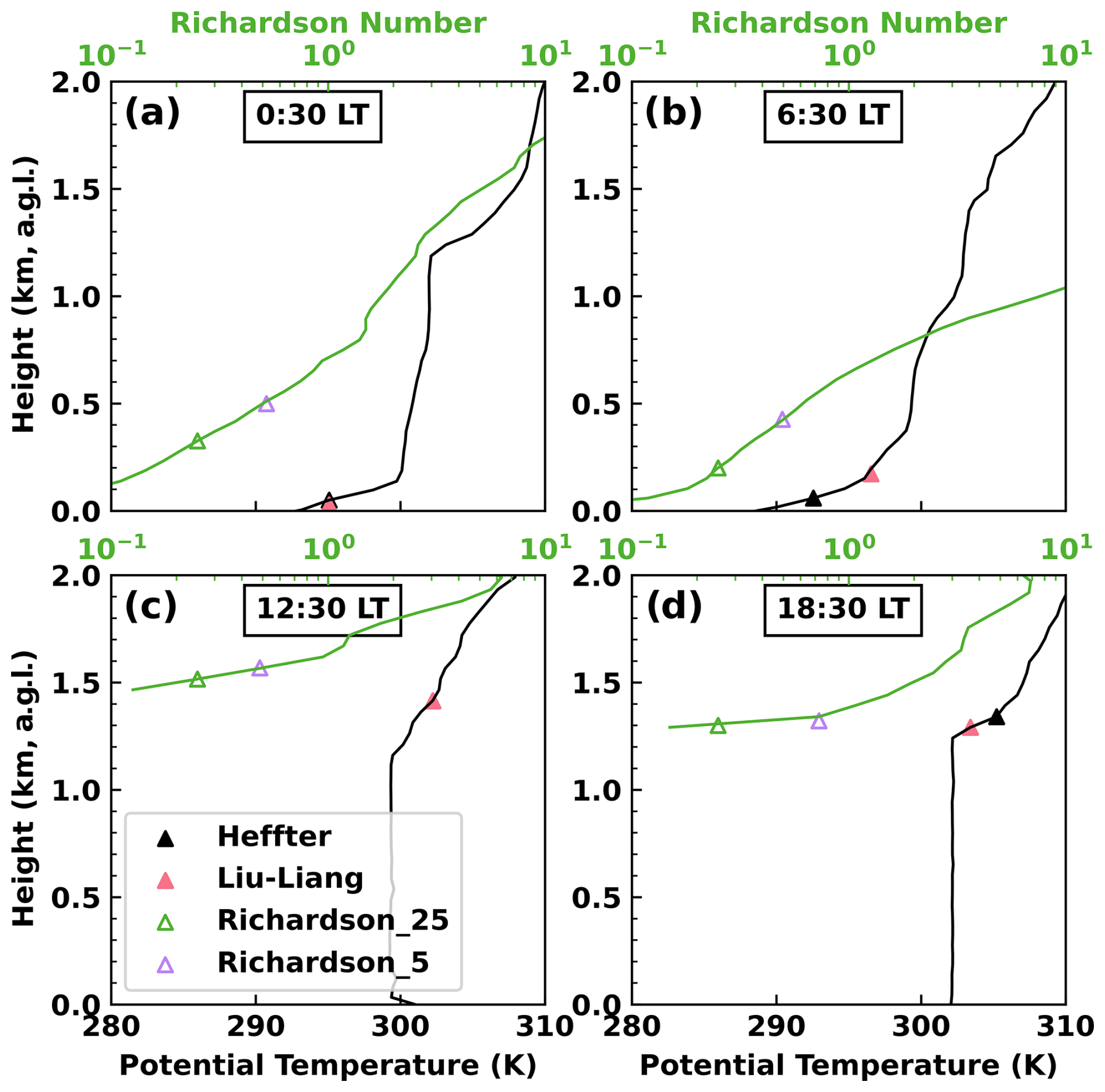
Figure 1 PBLHT estimates from the PBLHT-SONDE VAP during the four SONDE launches on 8 May 2017. Since PBLHTs from the Heffter and Liu–Liang methods primarily rely on potential temperature profiles, their PBLHT estimates are plotted alongside these profiles. PBLHTs from the bulk Richardson method are plotted on the corresponding Ri profiles. Richardson_25 refers to PBLHT estimate using an Ri_c threshold of 0.25, while Richardson_5 refers to an Ri_c threshold of 0.5. a.g.l. stands for above ground level, and all altitudes in this study are in terms of a.g.l.

Although PBLHT estimates from SONDE data are generally considered more reliable, there is no definitive ground truth to determine the method that performs better. Different methods and algorithms, even when using the same measurements, can yield significantly different PBLHT estimates (Seidel et al., 2010; Roldán-Henao et al., 2024a). This is evident in Fig. 1a and b, which show substantial discrepancies in PBLHT estimates from the PBLHT-SONDE VAP during nighttime (00:30 LT) and early morning (06:30 LT). Statistical comparisons of PBLHT estimates from the three approaches also reveal large discrepancies, particularly under stable PBL conditions (Figs. S1 and S2 in the Supplement). As a general rule, the median of PBLHT estimates from the three approaches is recommended (Smith and Carlin, 2024). Since the two PBLHT estimates from the bulk Richardson method use the same approach but with different Ri_c values, only the estimate with an Ri_c value of 0.25 is used when calculating the median PBLHT across the three approaches (Seibert et al., 2000).

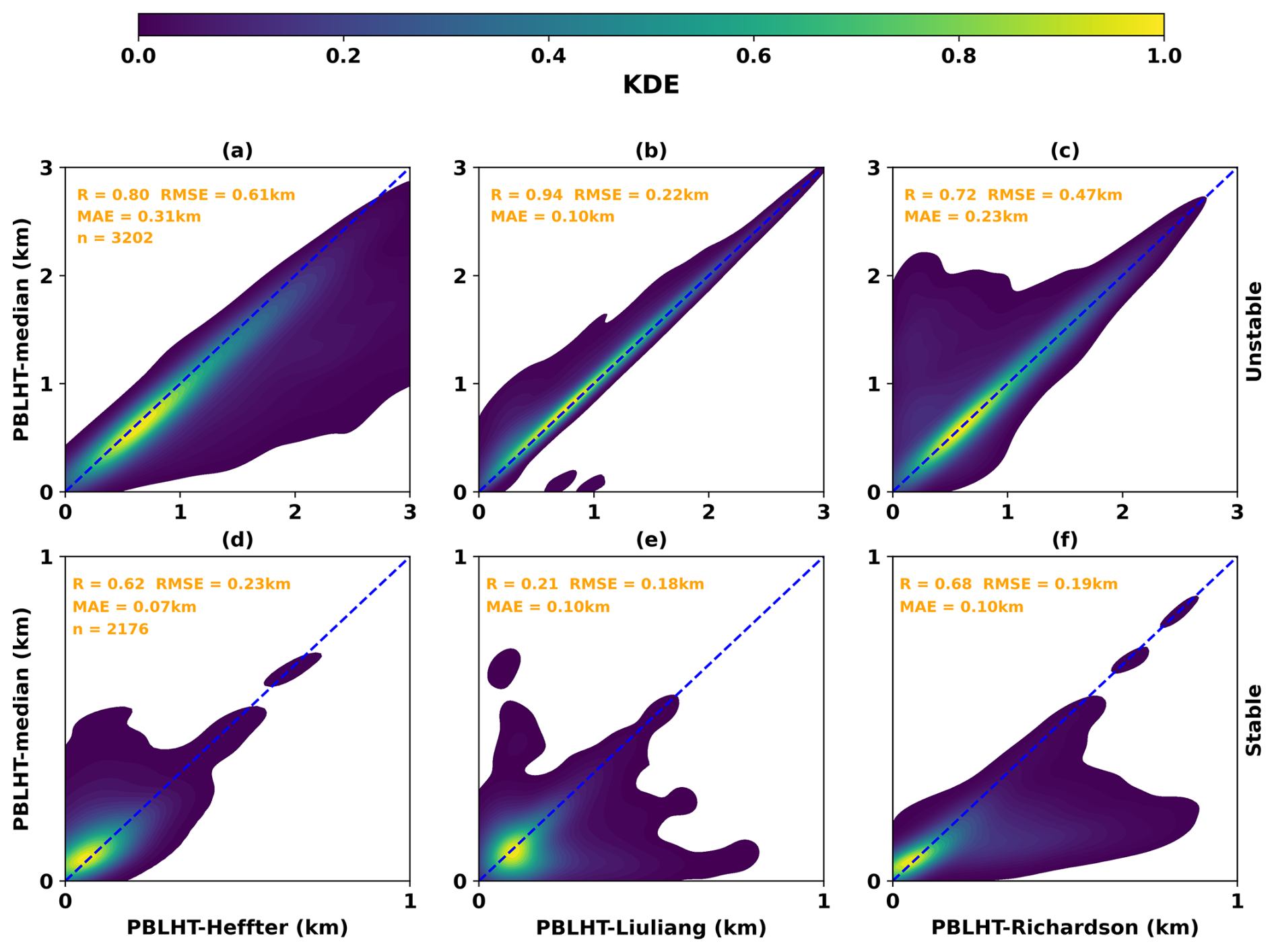
Figure 2 Comparisons of the three PBLHT estimates from the PBLHT-SONDE VAP with their median (PBLHT-median) using kernel distribution estimation (KDE) under unstable (a–c) and stable (d–f) PBL conditions. R is the correlation coefficient. RMSE is the root-mean-square error. MAE is the mean absolute error. n is the number of samples.

This study uses three parameters to evaluate how well two datasets are compared: the linear correlation coefficient (R), the root-mean-square error (RMSE), and the mean absolute error (MAE). Figure 2 shows this evaluation and compares the three PBLHT estimates from the PBLHT-SONDE VAP with their median (PBLHT-median) using kernel density estimation (KDE). KDE is a nonparametric technique used to estimate the probability density function of a continuous random variable. It provides a smooth approximation of the data distribution, making it useful for identifying patterns and trends (Zhang et al., 2022). Peaks in the KDE plot indicate regions with higher data density. Under unstable PBL conditions, the PBLHT-Liuliang estimate tends to align closely with the PBLHT-median, which shows the highest R and the lowest RMSE and MAE values. When PBLHT exceeds 2 km, PBLHT-Heffter is generally larger than the PBLHT-median, whereas PBLHT-Richardson is typically smaller than the median when PBLHT is below 1 km. On the other hand, under stable PBL conditions, the PBLHT-median is more likely to resemble either the PBLHT-Heffter or the PBLHT-Richardson estimates. These patterns are consistent with those of previous studies. For example, research using aerosol lidars and Doppler lidar (DL) suggests that PBLHT estimates from lidar are more in line with the Liu–Liang method during daytime at the SGP site (Sawyer and Li, 2013; Su et al., 2020; Krishnamurthy et al., 2021). Additionally, Lewis (2016) found that the Heffter method produces reasonable PBLHT values based on careful inspection of temperature and humidity profiles during the Marine ARM GPCI¹ Investigation of Clouds (MAGIC) field campaign. Seibert et al. (2000) noted that the bulk Richardson number method offers better PBLHT estimates under SBL conditions. In this study, we use the PBLHT-median as the “ground truth” to train and test ML models. For simplicity, in the following sections, we refer to the PBLHT-median as PBLHT-SONDE.

2.3 PBLHTs from remote sensing measurements

In this section, we describe four PBLHT estimates derived from remote sensing observations: PBLHT-MPL, PBLHT-CEIL, PBLHT-DL, and PBLHT-THERMO.

2.3.1 PBLHT-MPL

PBLHT-MPL is estimated using range- and overlap-corrected MPL backscatter profiles with the wavelet covariance method, as described by Sawyer and Li (2013). The ARM MPL system provides aerosol backscatter intensity and depolarization ratio profile measurements at a wavelength of 532, with a vertical resolution of 15 m and a temporal resolution of 10 s. The raw data are post-processed to subtract background noise and apply dead time, after-pulse, and overlap corrections (Campbell et al., 2002). Figure 3a presents an example of MPL backscatter profiles from 8 May 2017 at the SGP site. Residual aerosol layers are clearly visible up to approximately 2 km during the nighttime and early-morning hours until 06:00 LT, with elevated aerosol layers above 2 km at the start of the day, which can lead to significant errors in lidar-based PBL retrievals (Su et al., 2020). After 11:00 LT, strong aerosol backscatter gradients at the top of the PBL are evident.

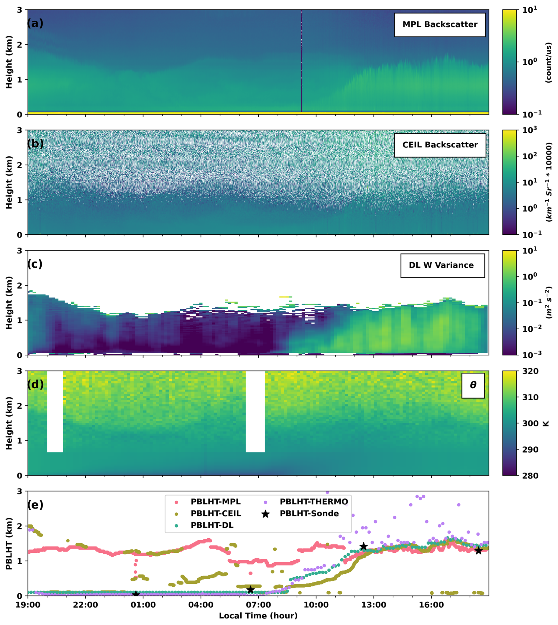
Figure 3 Remote sensing observations and retrievals on 8 May 2017 at the ARM SGP site. Panels from top to bottom are (a) time–height plot of MPL backscatter profiles, (b) ceilometer total attenuated backscatter coefficient profiles, (c) DL-derived vertical velocity variance (W) profiles, (d) potential temperature (θ) profiles from RL and TROPospheric Optimal Estimation (TROPoe) retrievals, and (e) PBLHT estimates from remote sensing observations and the PBLHT-SONDE VAP.

The Sawyer and Li approach uses the Haar wavelet covariance transform on the lidar backscatter intensity profile to identify the strongest negative gradient with height, which is then taken as the PBL top (Brooks, 2003). This wavelet covariance transform is an advanced edge detection technique well-suited for vertically resolved active remote sensing data. The method relies only on lidar backscatter intensity profiles and is independent of absolute lidar calibration, making it adaptable for different MPL systems across various locations. A key parameter in this approach is the dilation factor, a, of the Haar wavelet, which usually ranges between 100 m and 1 km. A small value of a may result in noisy PBLHT estimates due to spurious gradients, while large values increase the minimal detectable PBLHT. The minimal detectable PBLHT is half of a. Following Sawyer and Li (2013), we set the dilation factor, a, to 1 km, corresponding to a minimal detectable PBLHT of 0.5 km a.g.l. (above the ground level). Figure 3e shows that before 11:00 LT, PBLHT-MPL captures the top of the residual layer as the PBLHT, while after 11:00 LT, it accurately tracks the PBLHT of the convective PBL.

2.3.2 PBLHT-CEIL

In this study, we use ceilometer PBLHT estimates directly provided by vendor built-in software, “BL-View”, which provides real-time monitoring of boundary layer structures and identifies up to three potential boundary layer heights (Münkel and Räsänen, 2004). ARM ceilometers utilize the Vaisala CL31 model, which has a maximum vertical range of 7.7 km (Münkel and Räsänen, 2004). The CL31 provides total attenuated backscatter coefficient profiles at a wavelength of 910 nm, with a vertical resolution of 10 m and a temporal resolution of 2 s. Figure 3b shows the time–height plot of CEIL backscatter profiles. Due to longer wavelengths, a larger field of view, and stronger water vapor absorption, CEIL backscatter profiles tend to be noisier compared to those from MPL. Despite this, aerosol layer structures are still discernible within the PBL (Wiegner et al., 2019).

The CL31 ceilometer estimates PBLHT using the gradient method, which identifies local gradient minima, i.e., the strongest decrease in ceilometer backscatter with respect to altitude, in the range- and overlap-corrected backscatter coefficient profiles. First, the data are averaged to a 16 s temporal resolution to improve the aerosol signal reliability. Then, local gradient minima are detected using a 30 min temporal- and 360 m vertical-sliding-window average. Furthermore, the enhanced gradient method applies a cloud and precipitation filter during the averaging process to suppress false layer identification. This allows for robust PBLHT estimates under various weather conditions (Münkel and Roininen, 2010). For the three potential boundary layer heights, the BL-View algorithm assigns a quality index (ranging from 1 to 3) to each boundary layer height candidate. A higher quality index is assigned to stronger gradients, greater distances between minima, and scenes where no clouds are detected near the boundary layer. We select the boundary layer height candidate with the highest quality index as the ceilometer-estimated PBLHT, consistent with previous studies (Zhang et al., 2022). If there is more than one PBLHT candidate that has the highest quality index, the lower-altitude PBLHT candidate is selected as the ceilometer-estimated PBLHT.

As illustrated in Fig. 3e on the example day, the PBLHT-MPL consistently identifies the top of the residual layer as the PBLHT before 11:00 LT. In contrast, the PBLHT-CEIL sometimes detects lower PBLHTs that are closer to those of PBLHT-SONDE. After 11:00 LT, when the convective PBL develops, PBLHT-CEIL typically captures PBLHT accurately, although occasional underestimations still occur. Since ceilometers are cost-effective, portable, and reliable, they are widely deployed at various ground-based atmospheric observatories. As a result, numerous studies have developed methods to improve PBLHT estimates from ceilometers (Caicedo et al., 2020; de Arruda Moreira et al., 2022). In this study, we directly use PBLHT-CEIL from the Vaisala BL-View software, as it is readily available at ARM observatories, is quality-controlled, and has been widely adopted by the research community.

2.3.3 PBLHT-DL

ARM DL provides range-resolved measurements of attenuated backscatter intensity at approximately 1.5 µm and radial velocity profiles. Most ARM DLs have full upper-hemispheric scanning capabilities and typically operate in a vertical staring mode, offering vertical velocity measurements with a resolution of 30 m and a temporal resolution of 1 s or less. Additionally, they perform plan–position-indicator (PPI) scans to capture three-dimensional turbulent flows (Newsom and Krishnamurthy, 2022). The Doppler Lidar Vertical Velocity Statistics (DLPROF-WSTATS; https://arm.gov/capabilities/science-data-products/vaps/dlprof-wstats, last access: 21 September 2024) VAP uses vertical velocity data to calculate 30 min statistics of vertical velocity variance (${\mathit{\sigma }}_w^{\mathrm{2}}$), skewness, and kurtosis. The vertical velocity profiles are oversampled by a factor of 3 to produce these statistical quantities at a 10 min temporal resolution. Figure 3c shows the time–height plot of ${\mathit{\sigma }}_w^{\mathrm{2}}$. During nighttime, the stable atmospheric stratification created by radiative cooling leads to negative buoyancy production, effectively suppressing turbulence. ${\mathit{\sigma }}_w^{\mathrm{2}}$ remains low at night and in the early morning, while during daytime, enhanced convection increases surface-based mixing and increases atmospheric turbulence. As a result, ${\mathit{\sigma }}_w^{\mathrm{2}}$ starts to increase after 08:00 LT.

According to Tucker et al. (2009), the depth of the convective boundary layer can be estimated by identifying the height where ${\mathit{\sigma }}_w^{\mathrm{2}}$ falls below a specified threshold, such as 0.04 m² s⁻², which is the approach used in this study to derive PBLHT-DL from DLPROF-WSTATS. Figure 3e shows that PBLHT-DL reports lower PBLHT values before 08:00 LT, which aligns closely with the results from PBLHT-SONDE. However, during this period, PBLHT-DL consistently reports the lowest levels, indicating its limitations in providing valid PBLHT estimates under stable PBL conditions. Between 08:00 and 12:00 LT, PBLHT-DL effectively captures PBL growth, offering valuable PBLHT estimates during this critical period. After 12:00 LT, PBLHT-DL continues to provide reasonable PBLHT estimates, closely matching those of PBLHT-SONDE.

2.3.4 PBLHT-THERMO

At night, the presence of residual layers can create strong water vapor and aerosol gradients, making it difficult to derive PBLHT from water vapor or aerosol lidar backscatter profiles. Under such conditions, PBLHT estimates based on thermodynamic profiles, such as potential temperature, are more reliable (Seidel et al., 2010; Ferrare et al., 2012). Both ARM RL and AERI provide height- and time-resolved temperature profiles that can be used for this purpose. The ARM RL is an advanced lidar system that measures elastically backscattered light from aerosols at a wavelength of 355 nm, as well as inelastically scattered light from atmospheric molecules at specifically tuned channels. These measurements enable retrievals of the aerosol backscatter coefficient, water vapor mixing ratio, and temperature profiles (Newsom et al., 2013; Thorsen and Fu, 2015; Lv et al., 2017, 2018). Studies have previously demonstrated that RL-derived aerosol backscatter coefficient and water vapor profiles can be used to estimate PBLHT (Ferrare et al., 2012; Chu et al., 2022). However, due to known limitations of RL retrievals – such as artifacts in aerosol backscatter coefficients resulting from weak Raman scattering and periodic gaps in water vapor profiles – the authors chose not to incorporate the RL aerosol backscatter coefficient and water vapor mixing ratio profiles when estimating PBLHTs in this study. These issues could pose substantial challenges for automated PBLHT detection algorithms. The ARM Raman Lidar Temperature (RLPROF-TEMP; https://www.arm.gov/capabilities/science-data-products/vaps/rlproftemp, last access: 21 September 2024) VAP uses measurements from RL's rotational Raman channels to retrieve temperature profiles (Newsom et al., 2013). These temperature profiles have a vertical resolution of 60 m and a temporal resolution of 10 min (Newsom and Sivaraman, 2018). The uncertainty in the RL's temperature retrievals is calculated using standard error analysis, and by default, temperature retrievals with relative uncertainties greater than 0.05 are excluded. It is important to note that lidar signals and temperature retrievals can be affected by incomplete overlap between the outgoing laser beam and the receiver's field of view. As a result, overlap corrections are typically applied at low altitudes, where retrievals have higher uncertainties.

The ARM AERI retrieves boundary layer temperature profiles, which can also be retrieved from the measured infrared (IR) radiance spectrum. The ARM AERI instrument measures absolute IR spectral radiance from wavenumbers 3000 to 520 (cm⁻¹) with a spectral resolution of 1 cm⁻¹, with data collected every 20 s. The ARM TROPospheric Optimal Estimation (TROPoe) VAP (https://www.arm.gov/capabilities/science-data-products/vaps/tropoe, last access: 21 September 2024) provides retrievals of lower-tropospheric temperature and water vapor mixing ratio profiles from AERI IR spectral radiance measurements using a physical–iterative retrieval approach, as described by Turner and Löhnert (2014, 2021). TROPoe retrievals are produced at a 5 min temporal resolution, with vertical resolutions starting at approximately 25 m near the surface and decreasing to 800 m by 3 km in altitude. The output file also includes the 1σ uncertainty for each retrieved variable derived from the error covariance matrix within the optimal estimation framework. The mean bias errors relative to radiosonde profiles are less than 0.2 K for temperatures at heights below 2 km under clear-sky conditions (Turner and Löhnert, 2014).

To address the impact of overlap correction on RL temperature retrievals and to leverage the higher vertical resolution of TROPoe near the surface, we combine the RLPROF-TEMP and TROPoe temperature profiles. Specifically, TROPoe temperatures are used for altitudes below 700 m. At altitudes between 700 and 1100 m, RLPROF-TEMP temperatures are linearly scaled using the ratio of the mean TROPoe temperature to the mean RLPROF-TEMP temperature within this layer. RLPROF-TEMP temperatures are applied to altitudes above 1100 m. Potential temperature (θ) profiles are then calculated using the combined temperature profiles, along with pressure profiles from the interpolated SONDE (INTERPSONDE) VAP (https://www.arm.gov/capabilities/science-data-products/vaps/interpsonde, last access: 21 September 2024). Figure 3d displays the time–height plots of the θ profiles. PBLHT-THERMO is derived from these θ profiles using the Heffter method. The Liu–Liang and bulk Richardson number methods were not included because they require high-quality temperature and low-level wind data, which are limited by the capabilities of ARM Doppler lidar measurements. As shown in Fig. 3e, PBLHT-THERMO reports lower PBLHT values before 08:00 LT. Notably, PBLHT-THERMO indicates that the PBL begins to grow around 07:30 LT, while PBLHT-DL shows noticeable PBL growth after approximately 08:30 LT. This discrepancy may arise because thermodynamic measurements are more effective for estimating PBLHT than dynamic measurements in shallow, stable PBL conditions. After 12:00 LT during convective PBL, PBLHT-THERMO exhibits more scattered estimates, likely due to greater uncertainties in temperature retrievals and smaller potential temperature gradients at higher altitudes.

2.4 Statistical evaluations of PBLHT estimates from remote sensing measurements against PBLHT-sonde

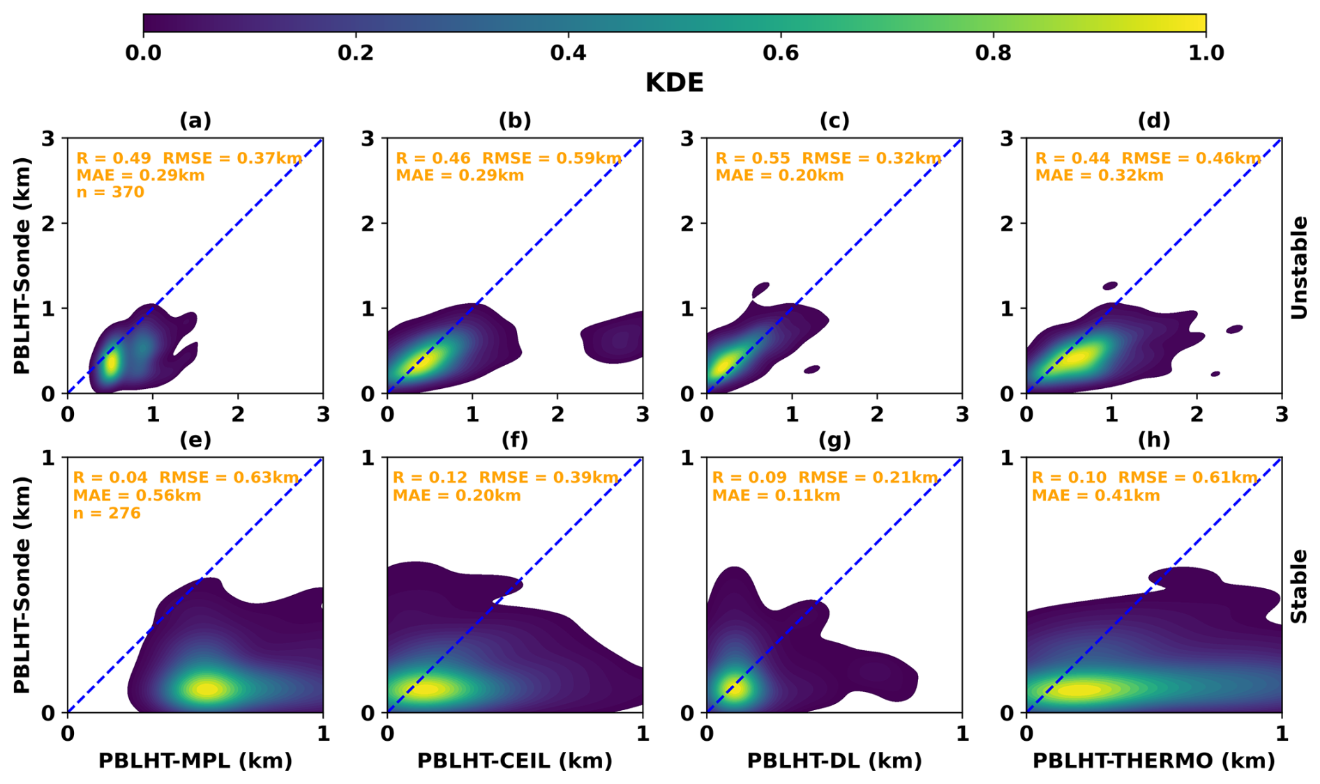
With multiple years of concurrent MPL, CEIL, DL, RL, TROPoe, and radiosonde data at the SGP site, we can statistically evaluate the performance of each PBLHT estimate from remote sensing measurements with PBLHT-SONDE. Figure 4 shows comparisons of the four PBLHT estimates from remote sensing measurements and PBLHT-SONDE under unstable and stable PBL conditions using 7 years of data between 2017 and 2023 at the SGP site.

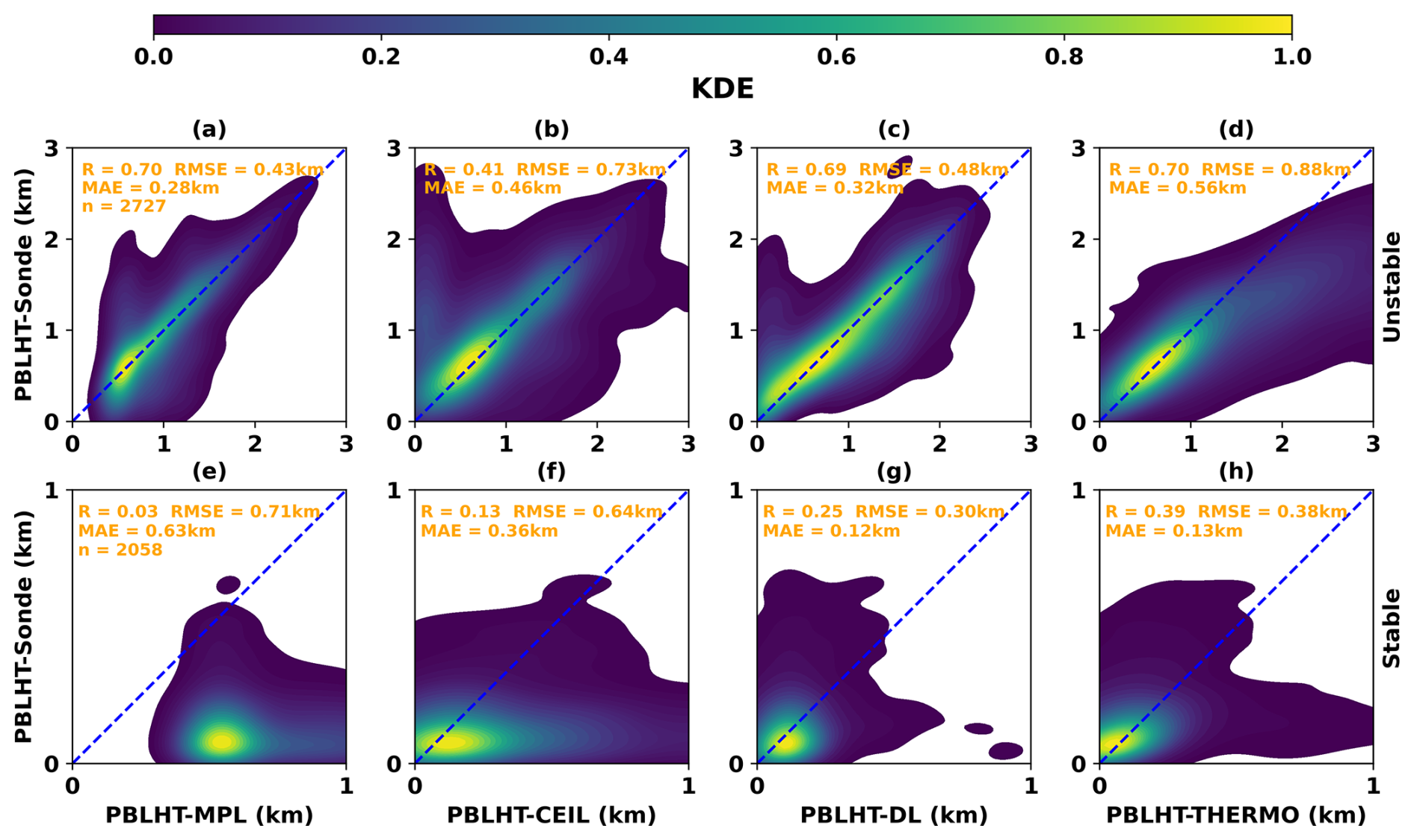
Figure 4 Comparisons of the four PBLHT estimates from remote sensing measurements with PBLHT-SONDE under unstable (a–d) and stable (e–h) PBL conditions. Note that different axis ranges are used for the unstable and stable PBL conditions.

Under unstable PBL conditions, both PBLHT-MPL and PBLHT-DL show better performance, with relatively higher R and lower RMSE and MAE values. PBLHT-MPL exhibits a smaller spread around PBLHT-SONDE but is unable to detect PBLHT values below 0.5 km. In contrast, during unstable conditions, PBLHT-CEIL performs poorly, with the lowest R and relatively higher RMSE and MAE values due to a larger spread around PBLHT-SONDE. PBLHT-DL, while showing a good correlation with PBLHT-SONDE across all PBLHT ranges, has a larger spread compared to PBLHT-MPL for PBLHTs larger than 0.5 km. PBLHT-THERMO performs well for PBLHT values below 1 km but significantly overestimates PBLHT for values above 1 km, leading to the highest RMSE and MAE values among the four PBLHT estimates. The overestimation of PBLHT is likely due to the use of the Heffter method in PBLHT-THERMO, which tends to yield higher values compared to PBLHT-median, as shown in Fig. 2a. Additionally, greater uncertainties in temperature retrievals and weaker potential temperature gradients at higher altitudes may further contribute to the overestimation.

The performance of the four PBLHT estimates from remote sensing measurements deteriorates significantly under stable PBL conditions (Krishnamurthy et al., 2021; Su et al., 2020; Zhang et al., 2022), with much lower R values, as shown in Fig. 4e–h. The uncertainty in estimating PBLHTs from observations during stable atmospheric conditions has been documented in several studies (Su et al., 2020; Zhang et al., 2022). Reduced accuracy during nighttime is primarily attributed to the formation of the SBL, which generates smaller thermal gradients and weaker turbulence near the surface. These features are difficult to detect with remote sensing instruments due to weak or noisy returns (in terms of backscatter or scattering). In addition, PBLHTs can be shallow during nighttime conditions, wherein the PBLHT is below the lowest range gate for some of these remote sensing devices, making it hard to detect. Among the four methods, during stable conditions, PBLHT-DL and PBLHT-THERMO perform better than PBLHT-MPL and PBLHT-CEIL. PBLHT-MPL shows poor performance, with the lowest R and highest RMSE and MAE values, primarily due to its inability to detect PBLHT values below 0.5 km, while most PBLHT values under stable PBL conditions at SGP are below 0.5 km (Krishnamurthy et al., 2021). PBLHT-CEIL continues to exhibit a large spread around PBLHT-SONDE. PBLHT-DL has the lowest RMSE and MAE values, while PBLHT-THERMO achieves the highest R value.

The PBLHT-SONDE VAP does not explicitly account for the influence of clouds (Sivaraman et al., 2013). Similarly, PBLHT estimates derived from remote sensing also do not specifically consider the presence of clouds. To minimize the impact of mid- and high-level clouds, PBLHT detection algorithms are limited to within 4 km of the surface. Since low-level cloud bases generally occur at or near the PBLHT, detection algorithms often identify the cloud base as the PBLHT. This does not introduce significant errors when compared with PBLHT-SONDE (Sawyer and Li, 2013; Zhang et al., 2022). The above analysis reveals that no single remote sensing approach for estimating PBLHT consistently outperforms the others. Each method has unique strengths and limitations under different PBL conditions, primarily due to instrument constraints or retrieval uncertainties, as discussed in Sect. 1. However, these approaches are complementary, and integrating them can provide improved and more continuous PBLHT estimates.

3 Best-estimate PBLHT (PBLHT-BE)

3.1 PBLHT-BE from remote sensing measurements (PBLHT-BE-lidar)

To evaluate the hypothesis that combining PBLHT estimates from different remote sensing approaches can enhance PBLHT accuracy, we designed an idealized experiment. Among the four PBLHT estimates from remote sensing measurements, the closest to the “ground truth” – PBLHT-SONDE in this study – can be selected as the PBLHT-BE. Since all remote sensing methods include lidar measurements, the PBLHT-BE is referred to as PBLHT-BE-lidar. We manually searched for PBLHT-BE-lidar from the four remote-sensing-estimated PBLHTs by comparing them against PBLHT-SONDE at each radiosonde launch time. Figure 5 compares PBLHT-BE-lidar with PBLHT-SONDE, showing that, under both unstable and stable conditions, the R is significantly improved, to 0.97 and 0.85; the RMSE is greatly reduced, to 0.15 and 0.08 km; and the MAE is reduced, to 0.10 and 0.04 km, respectively. The data distributions of PBLHT-BE-lidar and PBLHT-SONDE largely fall within a narrower range relative to the 1 : 1 line. This suggests that carefully selecting the best estimate from multiple remote sensing measurements can significantly improve PBLHT accuracy compared to relying on a single remote sensing method. Please note that this experiment provides PBLHT-BE-lidar estimates only when PBLHT-SONDE data is available and cannot be applied to other time periods. Understanding when or under what conditions a specific PBLHT estimate from remote sensing measurements best aligns with PBLHT-SONDE and is selected as the PBLHT-BE-lidar is valuable. Figure 6 presents histograms of the probability distributions of PBLHT estimates from the remote sensing measurements selected as the PBLHT-BE-lidar at different local times (Fig. 6a) and under different PBL regimes (Fig. 6b). The results show that during nighttime and early morning, before 10:00 LT, or under stable PBL conditions, PBLHT-THERMO is more frequently chosen as the PBLHT-BE-lidar, followed by PBLHT-DL. After 12:00 LT or under unstable PBL conditions, PBLHT-DL and PBLHT-MPL are more likely to be selected as PBLHT-BE-lidar. These findings indicate that PBLHT-THERMO is more accurate during nighttime or early morning or under stable PBL conditions, whereas PBLHT-MPL and PBLHT-DL perform better in the afternoon or under unstable conditions, consistent with the patterns shown in Fig. 4.

Figure 5 Similar to Fig. 4 but for comparisons between PBLHT-BE-lidar and PBLHT-SONDE.

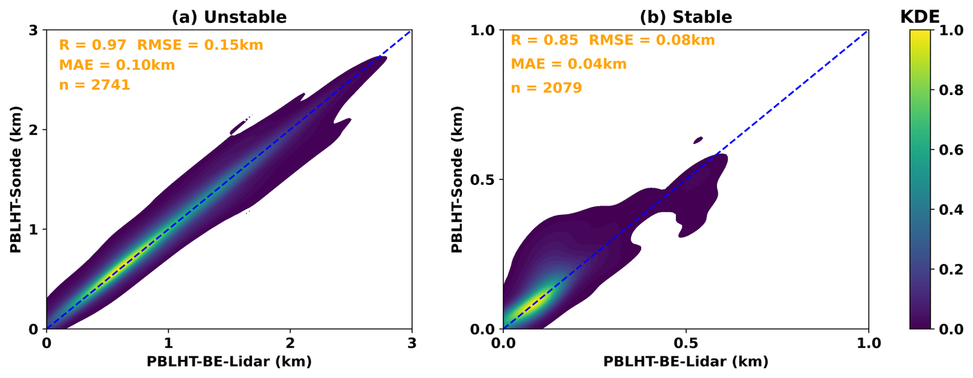
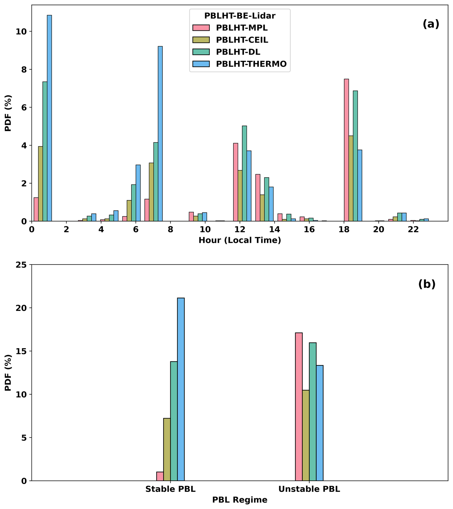
Figure 6 Histogram plots of probability distribution functions (PDFs) of PBLHT estimates from remote sensing measurements that are selected as the PBLHT-BE-lidar at different LTs (a) and under different PBL regimes (b).

3.2 PBLHT-BE using ML (PBLHT-BE-ML)

The discussion above highlights the need for an automated approach to derive more accurate PBLHT estimates from multiple remote sensing measurements when PBLHT-SONDE data are unavailable. This would allow for improved continuous PBLHT estimates, facilitating the study of PBL evolution and the evaluation of model simulations. To achieve this, we tested three machine learning models – RF classifier, RF regressor, and the light gradient-boosting machine (LightGBM – for predicting PBLHT. These models utilized four PBLHT estimates derived from remote sensing measurements along with the environmental variables listed in Table 1.

3.2.1 Data preparation and ML models

Remote sensing, radiosonde, and surface measurements, as summarized in Table 1 and collected between 2017 and 2023, are used to train and test ML models. Because radiosondes are routinely launched every 6 h, we find the closest remote sensing and surface data to the radiosonde launch time to create the concurrent observation dataset. For the ARM data products listed in Table 1 and the PBLHT estimates from remote sensing measurements, quality control (QC) flags are added for each variable. These QC flags are used to filter erroneous data or bad retrievals. Given that PBLHT estimates from the four lidar measurements are key input data, we also remove cases when a whole day of PBLHT estimates is missing from any lidar measurements. In total, 4785 PBLHT-SONDE estimates from radiosonde measurements were used for the training process. Following Krishnamurthy et al. (2021), we refer to the variables listed in Table 1 as input features. Missing data, often caused by instrument malfunctions or failures, are not uncommon in datasets that integrate a wide range of observational data streams. To address this, we apply the Pandas Python library forward- and backward-fill methods to handle missing values. The forward-fill method replaces missing data with the last known value, while the backward-fill method uses the next valid value moving backwards. To minimize mismatches caused by large data gaps, forward-fill and backward-fill methods were applied only within 1 h of missing data. Finally, we substitute the missing value with the average of the forward- and backward-filled values. Data standardization is commonly applied to enhance machine learning model performance (Sujon et al., 2024). However, random forest (RF) models and LightGBM are not sensitive to standardization or scaling (Breiman, 2001). As a result, we use the input features directly, without standardizing, for the training process.

The Scikit-Learn library for Python (Pedregosa et al., 2011) was used in this study for model hyperparameter tuning, training, and evaluation of machine learning algorithms. Hyperparameters are settings that govern the learning process of machine learning algorithms, influencing aspects such as the model complexity, learning rate, number of layers, and regularization. Optimal hyperparameter selection is essential to maximize model performance. This process is automated using Scikit-Learn's GridSearchCV, which conducts cross-validated hyperparameter tuning to determine the optimal model configuration. Hyperparameters optimized in this study were the number trees in the forest (n_estimators), the maximum number of features to consider when looking for the best split (max_features), the maximum number of splits each tree can take (max_depth), and the maximum number of leaf nodes a single decision tree within the forest can have (max_leaf_nodes). Model training and testing data are split randomly using Scikit-Learn's train_test_split function. 75 % of the data are used for training and the rest for testing the model.

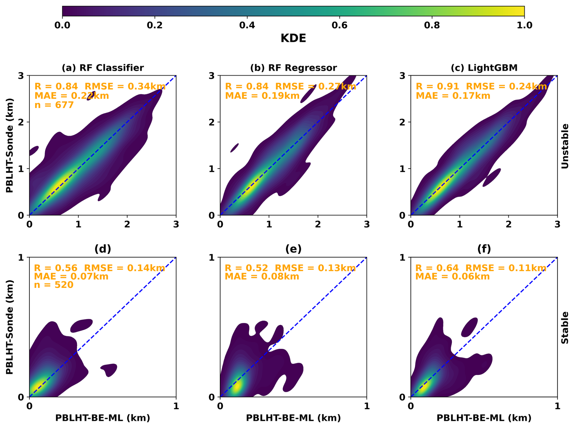
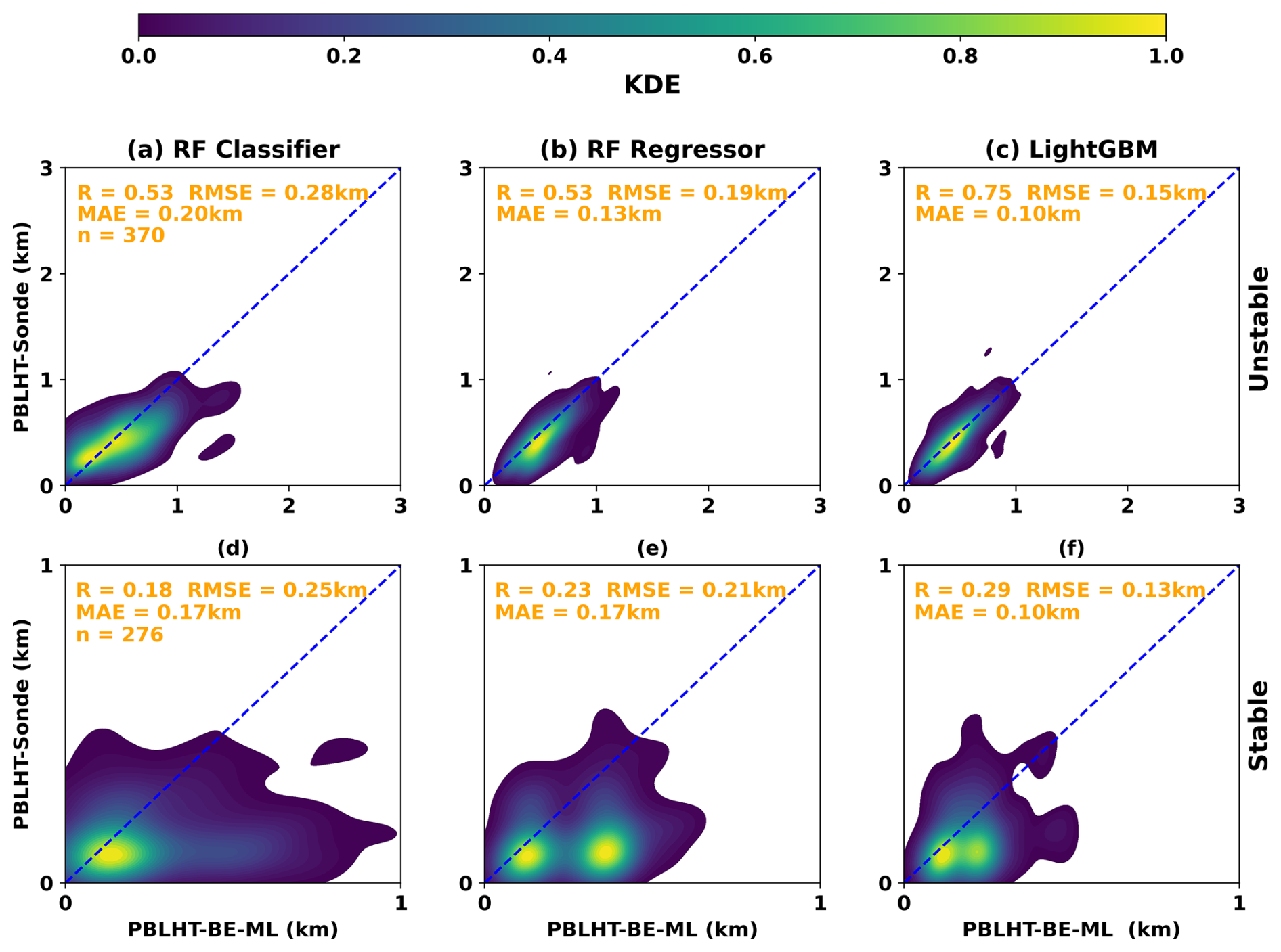
Figure 7 Similar to Fig. 4 but for comparisons between PBLHT-BE-ML predicted from ML methods and PBLHT-SONDE.

We first train an RF classifier model to find the PBLHT-BE (PBLHT-BE-ML), defined as the PBLHT estimate that is the closest to PBLHT-SONDE from the four lidar-based PBLHTs. The RF classifier is an ensemble machine learning model that builds multiple decision trees during training and merges their results to improve classification accuracy and reduce overfitting (Breiman, 2001). This ensemble ML approach helps improve the robustness and accuracy of predictions by reducing variance and leveraging the collective output of individual trees. Vertically resolved profiles of atmospheric state variables (e.g., temperature, water vapor, and vertical velocity) and tracers (e.g., aerosol particles) from remote sensing measurements can be used to reliably detect atmospheric features such as temperature and water vapor inversion layers, as well as aerosol layers. However, identifying the feature that is most closely related to PBLHT remains a challenge. The RF classifier model offers an effective solution to address this challenge. It has been widely used in many fields due to its high accuracy, flexibility, and ability to handle complex datasets. Figure 7a and d present evaluations of the predicted PBLHT-BE-ML from the RF classifier model compared with PBLHT-SONDE under both unstable and stable PBL conditions using the testing dataset. When compared to the PBLHT estimates derived from the individual remote sensing measurements shown in Fig. 4, the predicted PBLHT-BE-ML, which uses multi-remote sensing estimates, demonstrates a significantly higher correlation (R) and lower root-mean-square error (RMSE) against PBLHT-SONDE under both regimes. This indicates that the ML approach provides more accurate PBLHT estimates from integrated remote sensing data than estimates based on single remote sensing measurements do.

However, the R (RMSE) value between the predicted PBLHT-BE-ML from the trained RF classifier model and PBLHT-SONDE is lower (larger) than that of the idealized PBLHT-BE-lidar shown in Fig. 5. To address this, we tested other ML models, including the RF regressor and the light gradient-boosting machine (LightGBM) regressor models. Similar to the RF classifier model, the RF regressor is an ensemble learning model that uses averaging to enhance predictive accuracy and to control overfitting. The RF regressor extends the principles of the RF classifier to regression tasks by fitting multiple decision tree regressors to various subsamples of the dataset in order to predict continuous outcomes (Breiman, 2001). LightGBM is a widely used decision-tree-based ML model known for its speed, efficiency, and high performance (Ke et al., 2017). Unlike other boosting algorithms, LightGBM constructs decision trees leaf-wise instead of level-wise, enabling it to achieve lower losses and higher accuracy. Figure 7b, c, e, and f show the evaluations of the predicted PBLHT-BE-ML from the RF regressor and LightGBM models compared with PBLHT-SONDE under both unstable and stable PBL conditions. Overall, the RF regressor model performs similarly to the RF classifier, with the predicted PBLHT-BE-ML from the RF regressor showing a narrower data distribution relative to the 1 : 1 line and a lower RMSE compared to the RF classifier under unstable PBL conditions (Fig. 7b), indicating a slight performance advantage. The LightGBM regressor model outperforms both RF models, demonstrating the highest R and lowest RMSE values in evaluations against PBLHT-SONDE for both unstable and stable PBL conditions (Fig. 7c and f). The LightGBM model's predicted PBLHT-BE-ML shows substantially better correlations with PBLHT-SONDE than the RF models do and approaches the ideal PBLHT-BE depicted in Fig. 5.

Understanding whether the significant improvement in predicted PBLHT-BE-ML is due to the use of ML methods or the combination of various PBLHT estimates is important. Figures S3 and S4 show evaluations of predicted PBLHT using RF and LightGBM regressors based on individual remote sensing PBLHT estimates. The results indicate that ML models applied to individual remote sensing PBLHT estimates can also lead to substantial improvements in PBLHT prediction. However, there are several advantages to using multiple remote sensing data sources with ML models: (1) it can further enhance predicted PBLHT accuracy, as evidenced by comparing Fig. 7 with Figs. S3 and S4; (2) it allows for more reliable PBLHT predictions during periods outside of routine radiosonde launch times, as will be discussed in Sect. 3.2.3; and (3) it enables consistent and reliable PBLHT predictions across different geographic regions, as will be shown in Sect. 3.2.4.

3.2.2 Feature importance analysis

Input features for the ML models, along with their abbreviations and source ARM data streams, are detailed in Table 1. We did not include a local time parameter in the input features because the parameter changes with the season and may have different relations with PBLHT at different locations, which could cause issues when using the ML prediction at other geographic locations. The quality and quantity of input features can significantly affect the model's accuracy and efficiency. Therefore, understanding the importance of input features is crucial for optimizing ML model performance. Scikit-Learn's random forest models have built-in feature importance metrics that help identify the input features that contribute most to the model's predictive power. This feature importance is calculated based on the average reduction in impurity each time a feature is used to split a node across all trees in the forest. Features causing substantial decreases in impurity are assigned higher importance scores and deemed more significant. These scores are normalized so that they sum to 1. The LightGBM model offers two main types of feature importance: “Split” and “Gain”. In this study, we use the Gain importance, which measures the improvement in the model's accuracy when a specific feature is used for splitting.

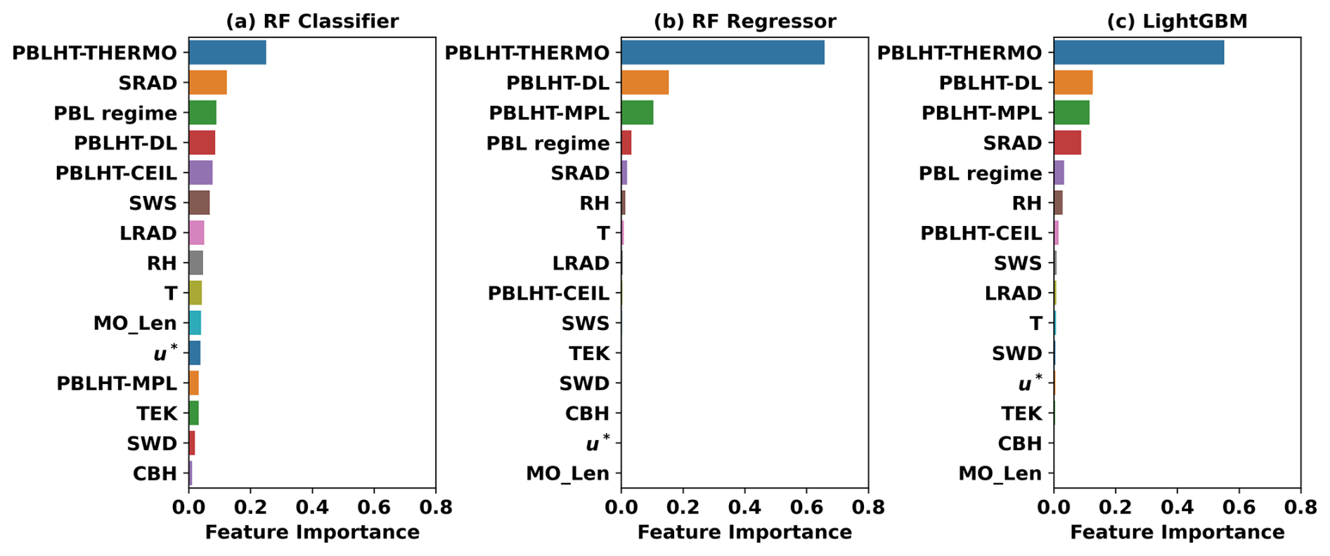
Figure 8 Feature importance for the three ML models at the training stage: (a) the RF classifier, (b) the RF regressor, and (c) LightGBM. Feature importance scores are normalized so that they sum up to 1.​​​​​​​

Figure 8 shows the feature importance for the three ML models under all conditions. PBLHT-THERMO emerges as the most significant feature across all three models, likely because it uses potential temperature profiles to derive PBLHT and compares best with PBLHT-SONDE under stable PBL conditions and during nighttime or early morning, as demonstrated in Figs. 5 and 6. In the RF classifier, each input feature contributes to the model's decision-making, as the prediction involves selecting the most appropriate PBLHT estimate from the four remote-sensing-based estimates. Each input feature can influence this selection to varying degrees under different environmental conditions. In contrast, PBLHT-THERMO, PBLHT-DL, and PBLHT-MPL are the three most important features for the RF and LightGBM regressor models, followed by SRAD and the PBL regime. This is because these models aim to predict PBLHT by interpolating or extrapolating from the input features to produce an estimate that aligns closely with PBLHT-SONDE. Consequently, other atmospheric or surface parameters play less of a role in these models. PBLHT-CEIL, which uses aerosols as tracers similarly to PBLHT-MPL, has a smaller impact because CEIL is less sensitive to aerosols and typically has a lower signal-to-noise ratio compared to MPL. As a result, PBLHT-CEIL estimates are generally less accurate and play a minor role in the RF and LightGBM regressor models. Additionally, comparisons of feature importance between daytime and nighttime reveal that PBLHT-DL and PBLHT-MPL are the most influential features during daytime, whereas PBLHT-THERMO dominates the feature importance during nighttime for RF regressor and LightGBM model predictions (Fig. S5).

3.2.3 Applying PBLHT-BE ML to continuous remote sensing measurements

Once the ML models were trained and tested using PBLHT-SONDE data, they were applied to predict high-temporal-resolution PBLHT-BE-ML using PBLHT estimates from the various remote sensing measurements and environmental variables listed in Table 1. Since PBLHT-THERMO has the coarsest temporal resolution (10 min) among the four remote sensing PBLHT estimates, its time dimension was used as the reference for the predicted PBLHT-BE-ML. All other input features were aligned to this time dimension using the “nearest” data mapping principle. Figure 9 presents an example of PBLHT estimates from individual remote sensing measurements and ML model predictions for 12 July 2019 at the ARM SGP site, with PBLHT-SONDE estimates included for comparison. On this day, radiosondes were launched eight times due to an intensive-observation period (IOP) for testing a tethered balloon system at SGP. The PBLHT estimates from individual remote sensing measurements exhibit issues similar to those seen in the 8 May 2017 case shown in Fig. 3. The predicted PBLHT-BE-ML from the three ML models aligns well with all eight PBLHT-SONDE estimates and displays a smooth, complete diurnal evolution of the PBLHT, as shown in Fig. 9b. The RF classifier model, however, shows abrupt jumps during the PBL growth period around 20:00 and 09:00 LT, which is probably caused by the transition of PBL regimes and/or quick changes in SRAD. In contrast, the RF regressor and LightGBM regressor models demonstrate smooth PBL growth during these periods.

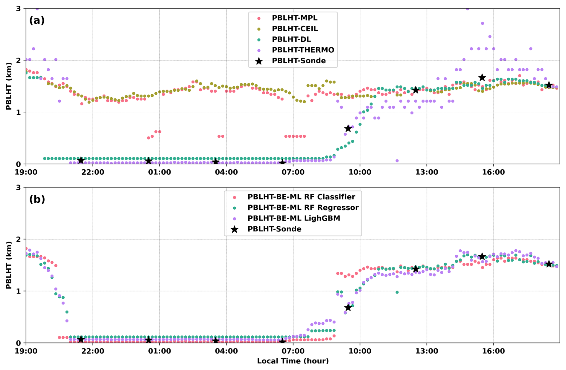
Figure 9 PBLHT estimates on 12 July 2019 at the ARM SGP site: (a) PBLHT estimates from individual remote sensing measurements and PBLHT-SONDE and (b) PBLHT-BE-ML prediction from the three ML models and PBLHT-SONDE.

High-temporal-resolution PBLHT estimates are crucial for studying the daily diurnal evolution of PBLHT as well as its seasonal variations. Figure 10 shows box and whisker plots of PBLHT diurnal cycles and their seasonal variations from the three ML model predictions and from PBLHT-SONDE at the ARM SGP observatory using data between 2017 and 2023. As expected, the comparison between PBLHT-BE-ML and PBLHT-SONDE is very good because 75 % of the data were used to train the ML models, and the validation using the remaining 25 % of the data shows good testing results, as presented in Sect. 3.2.1. Noticeable differences between PBLHT-BE-ML and PBLHT-SONDE occur at about 14:00 and 15:00 LT in fall, as shown in Fig. 10c, which is probably caused by small samples from a couple of IOPs. Clear PBLHT diurnal evolutions during all seasons are observed from all PBLHT estimation methods at the ARM SGP observatory, revealing a typical PBLHT diurnal evolution over the midlatitude land surface. The PBLHT remains shallow throughout the nighttime. It begins to grow around 09:00 LT, reaches its peak in the late afternoon, and starts to decay. Summer exhibits the highest convective PBLHT during the day and the lowest nighttime PBLHT compared to other seasons, likely due to the strongest daytime shortwave surface heating and the most intense nighttime longwave radiative cooling in this season. As a comparison, PBLHT diurnal cycles and their seasonal variations from PBLHT-MPL, PBLHT-CEIL, PBLHT-DL, and PBLHT-THERMO are shown in Fig. S6.

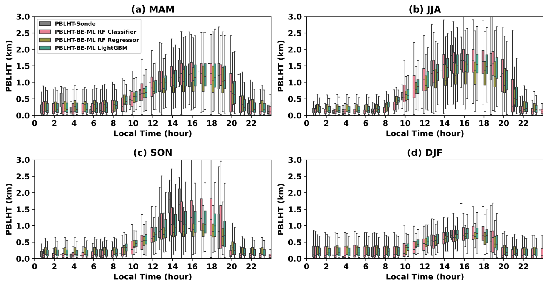
Figure 10 PBLHT diurnal cycles and their seasonal variations from the three ML model predictions and from PBLHT-SONDE at the ARM SGP observatory. MAM (March–April–May) represents the spring season, JJA (June–July–August) for summer, SON (September–October–November) for fall, and DJF (December–January–February) for winter. Horizontal bars, boxes, and whiskers represent the median, interquartile range, and range of the data.

The predicted PBLHT-BE-ML from the three ML models generally align well; however, they show notable differences under afternoon convective PBL conditions between 14:00 and 18:00 LT during summer and fall. The RF classifier predicts the highest PBLHT, while the RF regressor predicts the lowest. Unfortunately, we could not directly evaluate which model performs better due to the lack of routine radiosonde launches during this period. This highlights a general challenge for ML-based methods: how well do they perform when the target conditions differ from the training conditions? This period is characterized by strong turbulence within the PBL. Under such conditions, PBLHT estimates from aerosol lidars and Doppler lidars (DL) are considered reliable (Kotthaus et al., 2023) and show smaller relative standard deviations among different methods, as seen in Fig. S2b. Therefore, we can use lidar-derived PBLHT estimates to evaluate the ML model predictions. Similar to the method we used for different PBLHT estimates from radiosonde data, we calculate the median of PBLHT estimates from PBLHT-MPL, PBLHT-CEIL, and PBLHT-DL, referring to it as PBLHT-lidar. PBLHT-THERMO is excluded because it clearly overestimates PBLHT under strong convective conditions due to large uncertainties in temperature retrievals from RL measurements, as shown in Fig. 4d. We assume that PBLHT-lidar can be regarded as the “true” PBLHT under strong convective conditions and use it to evaluate the predicted PBLHT-BE-ML.

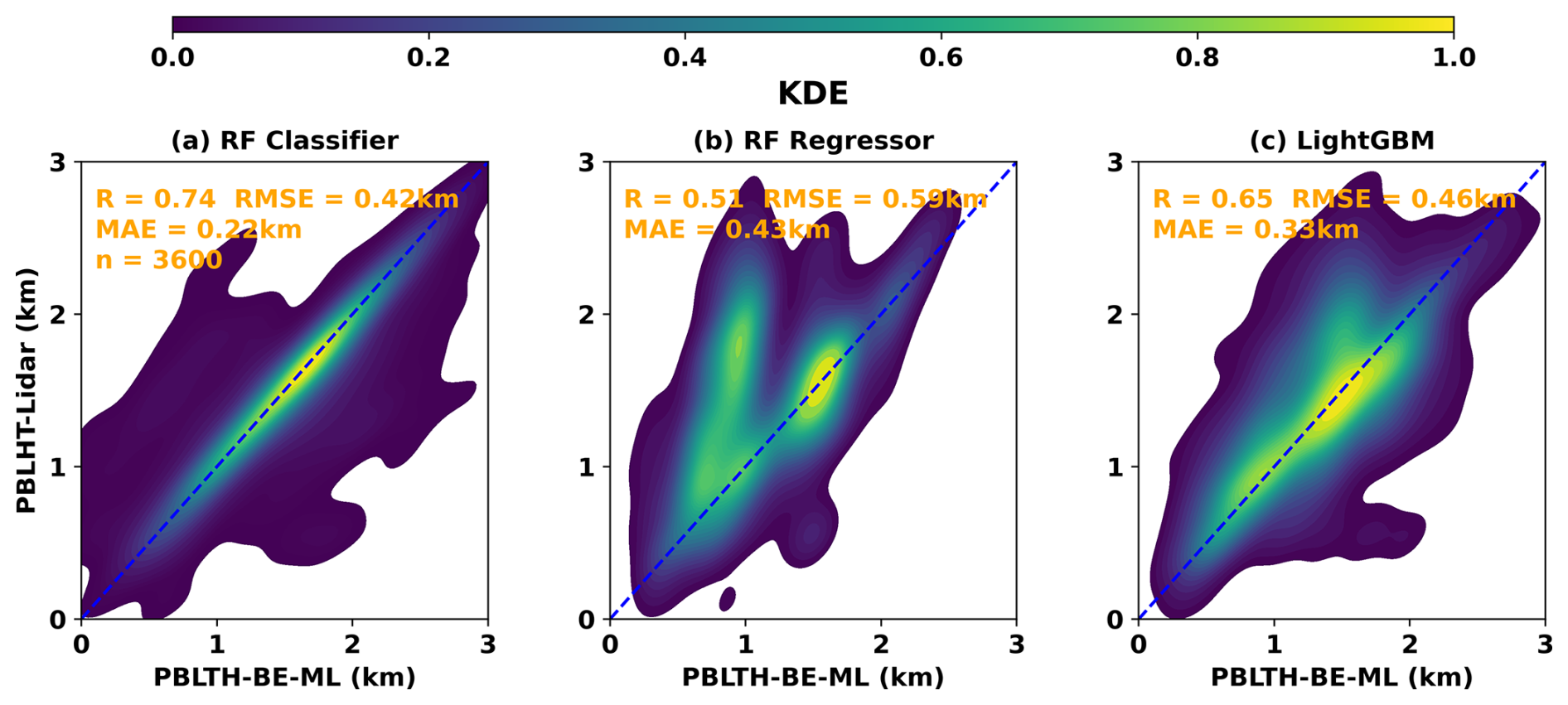
Figure 11 Similar to Fig. 4, except for comparisons between the predicted PBLHT-BE-ML and PBLHT-lidar from (a) the RF classifier, (b) the RF regressor, and (c) LightGBM under afternoon convective PBL conditions between 14:00 and 18:00 LT during summer and fall at the ARM SGP site.​​​​​​​

Figure 11 compares the predicted PBLHT-BE-ML from the three ML models with PBLHT-lidar. As expected, the agreement between predicted PBLHT-BE-ML and PBLHT-lidar is not as strong as during the radiosonde launch periods illustrated in Fig. 7. Among the three ML models, the RF classifier's predicted PBLHT-BE-ML shows the best agreement with PBLHT-lidar, with the highest R and lowest RMSE. The RF classifier's predictions closely align with the PBLHT-lidar along the 1:1 line, whereas the RF regressor and LightGBM predictions tend to be lower than both PBLHT-lidar and the RF classifier predictions, consistent with Fig. 10b and c. Additionally, the RF classifier's predicted PBLHT-BE-ML outperforms the best comparison between individual lidar PBLHT estimates and PBLHT-lidar, as shown in Fig. S7. To conclude, the performance of predicted PBLHT-BE-ML, particularly from regression-based ML models, may decrease when applied to periods that differ from the training data periods. More training data under afternoon convective PBL conditions are needed to improve ML model predictions. However, the classifier-based model remains effective at identifying the candidate PBLHT as the PBLHT-BE, providing enhanced predictions during afternoon convective PBL conditions.

3.2.4 Evaluation of predicted PBLHT-BE-ML at a different ARM site

To further evaluate the performance of the ML models in predicting PBLHT-BE, we compared the predicted PBLHT-BE-ML from the three ML models with PBLHT-SONDE data at a different ARM Mobile Facility (AMF) observatory. The ARM Eastern Pacific Cloud Aerosol Precipitation Experiment (EPCAPE) field campaign deployed an AMF at the Scripps Memorial Pier in La Jolla, California (the EPC site), from 15 February 2023 to 14 February 2024 (https://www.arm.gov/research/campaigns/amf2023epcape, last access: 21 September 2024). This field campaign focuses on characterizing the extent, radiative properties, aerosol interactions, and precipitation characteristics of stratocumulus clouds in the eastern Pacific at a coastal location, making PBLHT a critical parameter for understanding these processes. The EPC site is dominated by low-level marine stratocumulus clouds year-round, representing markedly different meteorological conditions compared to the SGP site. The deployment includes most instruments listed in Table 1, except for the RL. Consequently, PBLHT-MPL, PBLHT-CEIL, and PBLHT-DL for EPCAPE are derived in the same manner as at the SGP site. However, PBLHT-THERMO is derived solely using TROPoe data.

Figure 12 Similar to Fig. 4, except for the EPC site.

Turbulence over a warm ocean surface is generally weaker and exhibits less diurnal variability than over land, making it more challenging to obtain reliable PBLHT estimates in marine environments. Figure 12 presents comparisons of PBLHT estimates from various remote sensing measurements against PBLHT-SONDE at the EPC site. These comparisons are noticeably weaker than those observed at the SGP site (Fig. 4), as indicated by significantly lower correlation coefficients (R) at the EPC site. Additionally, PBLHT values under unstable PBL conditions at the EPC site are markedly lower than those at the SGP site, likely due to the limited thermal energy available for convection over the ocean. Among the different remote sensing PBLHT estimates, PBLHT-DL shows the strongest agreement with PBLHT-SONDE data under both unstable and stable PBL conditions, suggesting that PBLHT-DL may represent a reliable estimate for marine environments like the EPC site. PBLHT-THERMO performs best under stable PBL conditions at the SGP site; however, it consistently overestimates PBLHT compared to PBLHT-SONDE at the EPC site, which is likely due to large temperature retrieval uncertainties from TROPoe under opaque stratocumulus clouds. This discrepancy is likely due to higher uncertainties in potential temperature profile retrievals from TROPoe and the less distinct gradient in the potential temperature profile under stable (cloudy) PBL conditions at the EPC site.

Figure 13 Similar to Fig. 7, except for the EPC site.

We applied the three trained ML models directly to EPC data to evaluate their performance against PBLHT-SONDE. Figure 13 presents evaluations of the predicted PBLHT-BE-ML from the three ML models compared to PBLHT-SONDE under both unstable and stable PBL conditions. Compared to the PBLHT estimates from individual remote sensing measurements shown in Fig. 12, the predicted PBLHT-BE-ML from all three ML models shows improvement under both unstable and stable PBL conditions. Although the RF classifier and regressor models do not show an increase in R compared to PBLHT-DL under unstable conditions, they do demonstrate a notable reduction in RMSE and MAE. Additionally, both models show improvements in R, RMSE, and MAE under stable conditions. Among the three ML models, LightGBM exhibits the best performance against PBLHT-SONDE, with significantly higher R and lower RMSE and MAE than both the RF classifier and regressor, as well as compared to the individual PBLHT estimates from remote sensing measurements under both unstable and stable PBL conditions. However, it should be noted that the performance of the ML models at the EPC site is not as strong as at the SGP site. Expanding the training dataset to include data from different surface types, such as warm ocean surfaces and ice- and snow-covered areas, could further enhance the ML model's performance across diverse locations.

4 Summary and discussions

The planetary boundary layer height (PBLHT) is commonly determined using radiosonde data and remote sensing measurements. PBLHT estimates from radiosondes are generally considered more reliable and are commonly used to validate estimates from remote sensing. The Department of Energy (DOE) Atmospheric Radiation Measurement (ARM) program provides PBLHT estimates from radiosonde data through its PBLHT-SONDE value-added product (VAP), which includes three methods: (1) the Heffter method, (2) the Liu–Liang method, and (3) the bulk Richardson method with critical thresholds of 0.25 and 0.5. However, radiosonde data suffer from low temporal resolution and are subject to sampling error. In contrast, lidar and radiometer remote sensing instruments offer a high temporal resolution and continuous PBLHT estimates. ARM provides various PBLHT estimates from remote sensing measurements, including (1) PBLHT-MPL, derived from the wavelet covariance of the micropulse lidar (MPL) backscatter profile (Sawyer and Li, 2013); (2) PBLHT-CEIL based on the VAISALA CL31's enhanced gradient method; (3) PBLHT-DL based on the vertical velocity variance measured by Doppler lidar, using a threshold of 0.04 m² s⁻² (Tucker et al., 2009); and (4) PBLHT-THERMO, derived from Raman lidar (RL) and atmospheric emitted radiance interferometer (AERI) temperature profiles using the Heffter method. Each remote sensing approach has its own strengths and limitations. To achieve reliable PBLHT estimates throughout the day and under varying boundary layer conditions, we trained machine learning (ML) models on the PBLHT-SONDE VAP to produce the best-estimate PBLHT (PBLHT-BE) from multiple remote sensing measurements at the ARM SGP site.

Comparisons of the three PBLHT estimates from the PBLHT-SONDE VAP reveal substantial differences across various PBL conditions. To address this variability, we use their median as the “ground truth” for training and testing the ML models, referring to it as PBLHT-SONDE. Evaluations of PBLHT estimates from individual remote sensing methods at the ARM Southern Great Plains (SGP) site indicate that both PBLHT-MPL and PBLHT-DL perform well under unstable conditions, with higher correlation coefficients (R) and a lower root-mean -quare error (RMSE). PBLHT-THERMO performs accurately for PBLHT values below 1.5 km but significantly overestimates values above 1.5 km. Under stable PBL conditions, the accuracy of PBLHT estimates from remote sensing measurements made by all methods decreases substantially but varies among different methods of mixed performance at different times of the day, with PBLHT-DL and PBLHT-THERMO showing slightly better performance than PBLHT-MPL and PBLHT-CEIL, especially at nighttime and in the early morning.

We integrate the four PBLHT estimates from remote sensing measurements to identify the PBLHT estimate (referred to as PBLHT-BE-lidar) that best aligns with PBLHT-SONDE. In an ideal scenario where the PBLHT estimate closest to PBLHT-SONDE is accurately selected as PBLHT-BE-lidar, the comparison with PBLHT-SONDE improves significantly. During the nighttime, early morning, or under stable PBL conditions, PBLHT-THERMO is more frequently selected as the PBLHT-BE-lidar. In the afternoon or under unstable PBL conditions, PBLHT-DL and PBLHT-MPL are more commonly chosen as the PBLHT-BE-lidar at the SGP site.

Automated approaches using ML methods were tested to derive PBLHT-BE (PBLHT-BE-ML). Remote sensing, radiosonde, and surface measurements spanning 2017 to 2023 were utilized for training and testing the ML models. A total of 4785 PBLHT-SONDE estimates from radiosonde measurements were included in the training (75 %) and testing (25 %) processes. We tested three ML models: a random forest (RF) classifier, an RF regressor, and LightGBM. All three models demonstrated improved alignment of PBLHT-BE-ML with PBLHT-SONDE, yielding higher R and lower RMSE and MAE values compared to PBLHT estimates from individual remote sensing measurements. LightGBM, in particular, demonstrated the best performance against PBLHT-SONDE for both unstable and stable PBL conditions. Feature analysis for these models revealed that PBLHT-THERMO is the most significant feature across all three, with PBLHT-DL and PBLHT-MPL also ranking as important features for the RF and LightGBM regressor models.

The trained ML models were then applied to various lidar remote sensing measurements to predict high-temporal-resolution PBLHT-BE-ML. An example from an intensive-observation-period (IOP) day shows that the predicted PBLHT-BE-ML from all three models aligns well with the eight PBLHT-SONDE estimates, capturing a smooth, complete diurnal evolution of PBLHT. Seasonal analysis of the diurnal evolution reveals that summer has the largest diurnal PBLHT variation, while winter shows the smallest. The predicted PBLHT-BE-ML from the three ML models is generally consistent, except for noticeable differences under afternoon convective PBL conditions between 14:00 and 18:00 LT in summer and fall. Due to a lack of routine radiosonde launches during this period, we used the median of PBLHT-MPL, PBLHT-CEIL, and PBLHT-DL as the “true” PBLHT, referred to as “PBLHT-lidar”, for evaluating ML model predictions. The results indicate that the RF classifier predictions align closely with PBLHT-lidar along the 1 : 1 line, while the RF regressor and LightGBM predictions tend to be slightly lower than both PBLHT-lidar and RF classifier predictions, suggesting that additional training data under afternoon convective PBL conditions could enhance ML model accuracy.

To further assess model performance, we applied the trained ML models to remote sensing measurements from the ARM Eastern Pacific Cloud Aerosol Precipitation Experiment (EPCAPE) field campaign at the EPC site. Due to weaker turbulence over the warm ocean surface, obtaining reliable PBLHT estimates at the EPC site is more challenging. PBLHT estimates from individual remote sensing measurements show significantly lower correlation (R) at the EPC site than at the SGP site. However, the predicted PBLHT-BE-ML from all three ML models demonstrates improvement under both unstable and stable PBL conditions, with LightGBM showing the best agreement with PBLHT-SONDE. Nonetheless, model performance at the EPC site is not as robust as at the SGP site, highlighting the need to expand the training dataset to include data from diverse surface types, such as ocean-, ice-, and snow-covered surfaces. The PBLHT-BE-ML method is being developed as a VAP to improve PBLHT estimates at ARM sites, with plans to expand model training beyond the SGP site.