Hourly surface nitrogen dioxide retrieval from GEMS tropospheric vertical column densities: benefit of using time-contiguous input features for machine learning models

Launched in 2020, the Korean Geostationary Environmental Monitoring Spectrometer (GEMS) is the first geostationary satellite mission for observing trace gas concentrations in the Earth's atmosphere. Observations are made over Asia. Geostationary orbits allow for hourly measurements, which lead to a much higher temporal resolution compared to daily measurements taken from low-Earth orbits, such as by the TROPOspheric Monitoring Instrument (TROPOMI) or the Ozone Monitoring Instrument (OMI). This work estimates the hourly concentration of surface nitrogen dioxide (NO₂) from GEMS tropospheric NO₂ vertical column densities (VCDs) and additional meteorological features, which serve as inputs for random forests and linear regression models. With several measurements per day, machine learning models can use not only current observations but also those from previous hours as inputs. We demonstrate that using these time-contiguous inputs leads to reliable improvements regarding all considered performance measures, such as Pearson correlation or mean square error. For random forests, the average performance gains are between 4.5 % and 7.5 %, depending on the performance measure. For linear regression models, average performance gains are between 7 % and 15 %. For performance evaluation, spatial cross-validation with surface in situ measurements is used to measure how well the trained models perform at locations where they have not received any training data. In other words, we inspect the models' ability to generalize to unseen locations. Additionally, we investigate the influence of tropospheric NO₂ VCDs on the performance. The region of our study is South Korea.

1 Introduction

The concentration of nitrogen dioxide (NO₂) near the Earth's surface is of significant interest for several reasons. NO₂ is not only a precursor to health hazard and air pollutant ozone, but also a direct threat to human health. Moreover, it is linked to environmental issues such as acid rain; see, e.g., Jacob (2000).

At present, surface NO₂ is measured by networks of ground-based in situ monitoring stations. However, due to the limited number of such stations, they cannot provide global information about the surface NO₂ concentration. This limitation is one of the reasons why satellite remote sensing has become popular for deriving global estimates of surface NO₂. Satellites detect the fingerprint of NO₂ within the backscattered solar radiation due to its strong absorption of light in the wavelength range of 350–500 nm. One of the first studies on deriving surface NO₂ from remote sensing observations was conducted by Lamsal et al. (2008) across the USA and Canada. In their study, surface NO₂ was estimated by applying an assumed NO₂ vertical distribution calculated with a chemical transport model to tropospheric NO₂ vertical column densities (VCDs), where the tropospheric NO₂ VCDs were obtained from the Ozone Monitoring Instrument (OMI; Levelt et al., 2006). Numerous further studies followed, also utilizing chemical transport models and observations from satellites in low-Earth orbits. For example, we refer to the studies of Lamsal et al. (2010, 2013), Bechle et al. (2013), Wang and Chen (2013), Kharol et al. (2015), Geddes et al. (2016), Gu et al. (2017), and Cooper et al. (2020, 2022). Both OMI data and other observations have been considered, e.g., from the Global Ozone Monitoring Experiment (GOME; Burrows et al., 1999), the Scanning Imaging Absorption Spectrometer for Atmospheric Chartography (SCIAMACHY; Bovensmann et al., 1999), and the TROPOspheric Monitoring Instrument (TROPOMI; Veefkind et al., 2012).

During the last 10 years, machine learning approaches have received increasing attention in determining surface NO₂ from satellite remote sensing observations. One advantage is the shorter computation time once the model has been trained. Diverse machine learning models have been used for this task, exploiting not only tropospheric NO₂ VCDs as input, but also additional input features to improve the model's performance, such as meteorological parameters, traffic density, or population information. Studies that consider observations from satellites in low-Earth orbits have been conducted by, for example, Kim et al. (2017), Jiang and Christakos (2018), de Hoogh et al. (2019), Chen et al. (2019), Di et al. (2020), Qin et al. (2020), Kim et al. (2021), Chan et al. (2021), Dou et al. (2021), Ghahremanloo et al. (2021), Li et al. (2022), Wei et al. (2022), Huang et al. (2023), and Shetty et al. (2024). For a detailed review on the methods used, the input features included, the regions of consideration, and the achieved performance, we refer to the work of Siddique et al. (2024).

Satellites in low-Earth orbits, such as OMI and TROPOMI, pass over the same region in middle and low latitudes once a day, which means they can provide at best one measurement per day and location. If the area is cloud-covered during the time of observation, the measurement of lower-tropospheric gases is not accurate, which makes the data coverage even more limited. Since satellites in low-Earth orbits provide observations at most once a day, most studies either predicted surface NO₂ at this specific satellite observation time (e.g., Kim et al., 2017) or estimated daily (e.g., Di et al., 2020), monthly, or annual averages of surface NO₂. Nevertheless, it should be mentioned that there are a few studies that have estimated hourly NO₂. As an example, Kim et al. (2021) linearly interpolated daily tropospheric NO₂ VCDs to an hourly resolution, from which they estimated hourly surface NO₂ concentrations over Switzerland and northern Italy.

In contrast, geostationary satellites permanently observe – more or less – the same region, leading to more data points for a given location that can be used for a prediction algorithm of surface NO₂. In particular, these larger datasets make machine learning approaches even more attractive. The first geostationary satellite instrument for observing trace gas concentrations in the Earth's atmosphere is the Geostationary Environmental Monitoring Spectrometer (GEMS; Kim et al., 2020), which was launched in February 2020 by the Republic of Korea. It provides hourly measurements of radiances over 20 countries in Asia, including South Korea. Alongside GEMS, there exists only one other geostationary satellite that monitors trace gases, namely NASA's TEMPO, which was recently launched in April 2023 and is observing North America. A third geostationary satellite, ESA's Sentinel-4 mission, was launched in 2025 and monitors Europe.

Until now, only a few studies have been conducted on hourly surface NO₂ retrieval from geostationary observations: Zhang et al. (2023) presented a scientific GEMS NO₂ product (POMINO-GEMS), which empirically corrects for overestimation and stripe artifacts in the operational GEMS NO₂ product. They then converted their tropospheric NO₂ VCDs of 2021 over China to hourly surface NO₂ using a chemical transport model. Further studies that exploit machine learning approaches have been conducted over China. Yang et al. (2023b) used a random forest regressor to predict hourly surface NO₂ over China from GEMS radiance data at six wavelengths from the UV and visible bands, as well as some additional meteorological, temporal, and spatial features. Furthermore, a multi-output random forest was used to simultaneously predict five more air pollutants, such as ozone. Although prediction accuracy achieved by the multi-output model was slightly worse regarding surface NO₂, the overall training time for predicting all six pollutant concentrations was smaller. Ahmad et al. (2024) combined two machine learning models. First, a random forest was used to predict NO₂ mixing heights from meteorological input features. These were then fed into an extreme gradient boosting regressor, together with tropospheric NO₂ VCDs from GEMS, temporal variables, and meteorological variables. The study demonstrates the benefit of using NO₂ mixing height as input.

Hourly surface NO₂ has also been predicted from GEMS observations over South Korea, the region considered in this study. In the work of Lee et al. (2024), predictions were made for the whole year of 2022. Therein, the total amount of VCDs instead of tropospheric NO₂ VCDs was used as the only input of a (linear) mixed-effect model to predict surface NO₂. Their model is a piecewise-defined function whose output depends not only on the total column of NO₂, but also on the day and hour at which and region in which the prediction is to be made. For this, South Korea was divided into nine regions, which presumably leads to a more direct region-wise relationship between surface NO₂ and column densities of NO₂. In other words, implicitly, spatial and detailed temporal information is also exploited in their approach. This makes their model specialized to South Korea and the year 2022.

Another study that predicted surface NO₂ over South Korea was conducted by Tang et al. (2024). Therein, daily surface NO₂ concentrations instead of hourly surface NO₂ were predicted. Further, they did not use NO₂ column densities as input for a machine learning model. Instead, they inspected the influence of aerosol optical depth, which is part of the GEMS data products. Aerosol optical depth, together with surface NO₂ predictions from a chemical transport model and other features such as meteorological parameters, served as inputs for a random forest to estimate surface NO₂.

In order to train and evaluate machine learning models of surface NO₂, in situ NO₂ observations from ground-based networks are used. Within the literature, there are two frequently used strategies to evaluate the performance of a machine learning model in predicting surface NO₂. First, standard k-fold cross-validation is considered; see, for example, the works of Ghahremanloo et al. (2021), Chan et al. (2021), Yang et al. (2023b), and Ahmad et al. (2024). This means that the whole dataset is randomly split into k equally sized subsets. One of them serves as the test set, whereas the other k − 1 values are used to train the model. Training and testing are repeated k times, until each subset has served once as a test set. The average test performance (e.g., Pearson correlation) is calculated and represents the final evaluation of the model. For standard k-fold cross-validation, data from all available in situ stations are contained in both the training and the test datasets (with large probability). However, what if the trained model should afterwards predict surface NO₂ at a new location which has not contributed data to the training set? With the result from standard cross-validation, it would be impossible to say how reliable the model can generalize to this unseen location. It may have overfitted to the locations that it has dealt with during training. Therefore, if global charts covering large areas like the entirety of South Korea are desired, it would be more appropriate to evaluate the model's performance via so-called spatial k-fold cross-validation. This means the set of available in situ stations is divided into training and test stations, the model is trained with data from training stations only, and – finally – its performance in predicting surface NO₂ at the test stations is evaluated. Unsurprisingly, performance measured with spatial cross-validation is indeed worse compared to standard cross-validation, which has been observed, e.g., within the studies of Ghahremanloo et al. (2021), Chan et al. (2021), Yang et al. (2023b), and Tang et al. (2024). In our work we focus on spatial k-fold cross-validation, as we wish to inspect how well a model can generalize to unseen locations.

1.1 Goals of this study

Due to the hourly measurements GEMS provides over the same region, it is natural to ask whether one can benefit directly from the time resolution itself and not only from the resulting larger size of the dataset. Hence, we propose training a machine learning model φ that predicts surface NO₂ at a given location z and time t not only from corresponding tropospheric NO₂ VCD and meteorological data at time t, but also from $(k-\mathrm{1})\in {\mathbb{N}}_{\mathrm{0}}$ previous hours (ℕ₀ denotes the set of natural numbers including zero). This means the model is a mapping $\mathit{\phi }:{\mathbb{R}}^{pk}\to \mathbb{R}$, where p is the number of different features:

$$\begin{array}{rl}& \text{input}(z,t):=\left(\begin{array}{c}\text{tropospheric}{\mathrm{NO}}_{\mathrm{2}}\text{VCD}(z,t)\\ \mathrm{⋮}\\ \text{tropospheric}{\mathrm{NO}}_{\mathrm{2}}\text{VCD}(z,t-k+\mathrm{1})\\ \text{meteorological features}(z,t)\\ \mathrm{⋮}\\ \text{meteorological features}(z,t-k+\mathrm{1})\end{array}\right)\\ & ⟼\mathit{\phi }\left(\text{input}\right(z,t\left)\right)\approx \text{surface}{\mathrm{NO}}_{\mathrm{2}}(z,t).\end{array}$$

Here t − j refers to the time j hours before t, where $j\in \left\{\mathrm{0},\mathrm{1},\mathrm{\dots },k-\mathrm{1}\right\}$. In all that follows, k is also referred to as the time contiguity of the input features, as it determines how many times each input feature is included in the whole input vector. Note that k = 1 stands for the case in which only input features at current time t are included. Of course, one could also use features at later times t + j, but for simplicity and better readability, we focus on making predictions based on previous-time features in this work.

Our main aim is to inspect whether the performance of the model in predicting surface NO₂ at unseen locations will increase by using inputs with higher time contiguity k. Unseen locations are locations from which the model has not seen any training data. As it turns out, it is indeed beneficial to use larger time contiguity k>1 for the machine learning models considered, namely random forests and linear regressors. To the best of our knowledge, this observation has not been made in the literature yet. Regarding work on non-geostationary satellite data, the usage of time-contiguous tropospheric NO₂ VCDs is simply impossible, as only single measurements per day are available. We further carefully design experiments that are suitable for answering our main research question about the benefit of time-contiguous inputs. Last but not least, we inspect the influence of tropospheric NO₂ VCDs on the models' ability to predict surface NO₂ and their influence on the benefit of using time-contiguous inputs. This is of interest as it addresses the question of how useful and necessary satellite observations of NO₂ are for the prediction of surface NO₂ concentrations.

1.2 Outline

In Sect. 2 we describe the different sources of data included in our study. Furthermore, we describe the construction of the datasets used for training machine learning models in our study and give a mathematical description of these datasets. Afterwards, in Sect. 3.2 we describe the experiments that provide clear insights into the research questions, e.g., whether time-contiguous inputs can enhance the quality of surface NO₂ predictions. We also discuss different loss functions for measuring the performance of trained models on the test dataset. Section 4 serves as a quick recap of the machine learning models used in this study. Finally, we present and discuss the results of our experiments in Sect. 5.

2 Data

In our study, we exploit two data sources for the prediction of surface NO₂. The first source is tropospheric NO₂ VCDs derived from GEMS measurements, and the second is meteorological data from the ERA5 dataset (Hersbach et al., 2023). Further, measurements of surface NO₂ at in situ stations from the air quality network of South Korea serve as the ground truth in this study. This section begins with a brief description of these data sources, followed by a description of the data preprocessing steps. In particular, we explain how the VCDs were paired with ERA5 and in situ data and how time-contiguous datasets were constructed. For clarity, we provide mathematical definitions of these time-contiguous datasets.

2.1 Data sources

2.1.1 GEMS tropospheric NO₂ vertical column densities

GEMS is a UV–visible imaging spectrometer on board the geostationary satellite GK2B. At its launch on 18 February 2020, GEMS was the first geostationary air quality monitoring mission. GEMS is located over the Equator at a longitude of 128.2° E and covers a large part of Asia (5° S–45° N and 75–145° E) on an hourly basis. With four different scan modes, which all include South Korea, the field of regard (FOR) shifts westward with the Sun. During daytime, GEMS provides up to 10 observations over a given location according to the season and location, with a spatial resolution at Seoul of 3.5 km × 8 km. The GEMS irradiance and radiance measurements in the UV–visible spectral range can be used to derive column amounts of, for example, ozone (O₃), sulfur dioxide (SO₂), and NO₂, but also cloud and aerosol information (Kim et al., 2020). For this study, we use the tropospheric NO₂ VCD product.

During the time of this study, the operational GEMS L2 tropospheric NO₂ VCD product was available in v2. This version was evaluated by, e.g., Oak et al. (2024) and Lange et al. (2024), showing that it is high biased compared to the TROPOMI tropospheric NO₂ VCD product and ground-based tropospheric NO₂ VCD datasets. Additionally, the v2 product showed enhanced scatter. In preparation for the European geostationary instrument on Sentinel-4, the Institute of Environmental Physics at the University of Bremen (IUP-UB) has developed a scientific GEMS NO₂ product. The GEMS IUP-UB tropospheric NO₂ VCD v1.0 product was evaluated by Lange et al. (2024), showing good agreement with the operational TROPOMI NO₂ data and ground-based observations. Here, an earlier version (v0.9) of the same data product was used. Briefly, the retrieval is based on a differential optical absorption spectroscopy fit in the 405–485 nm spectral window, using daily GEMS irradiances as background spectra. The stratospheric correction is based on a variant of the STREAM algorithm of Beirle et al. (2016), and tropospheric vertical columns are computed using air mass factors by applying the tropospheric NO₂ profiles from the TM5 model run performed for the operational TROPOMI product (Williams et al., 2017). The TM5 model has an hourly temporal resolution with a spatial resolution of 1° × 1°. As the model a priori is interpolated in space and time, no obvious structures from the coarse model resolution are visible in the data, but the lack of detail may still impact the results. Cloud screening is based on the operational GEMS cloud product v2 and a threshold of 50 % cloud radiance fraction, but no additional cloud correction is performed. Each pixel has a quality indicator (qa value) based on fitting residuals, cloud fraction, and surface properties. Here, only data with the highest qa value (good fits, cloud radiance fraction below 50 %, no snow or ice detected) are used.

Further, the GEMS IUP-UB product does not yet have full error propagation. The tropospheric NO₂ VCD error is therefore estimated to be 25 %. The main uncertainty results from the assumptions used in the calculation of air mass factors, in particular for surface reflectivity, the NO₂ vertical profile, and aerosol loading. Uncertainties are expected to be larger in the morning when the boundary layer is shallow and smaller around noon and in the evening. Uncertainties introduced by the stratospheric correction can be important over clean regions but can be neglected over pollution hotspots.

2.1.2 Meteorological data

In order to predict surface NO₂, it would not be sufficient to use tropospheric NO₂ VCDs as the only source of information. This is because VCDs represent integrals over the entire troposphere, capturing contributions from NO₂ at various altitudes, not just near the surface. A common strategy is to incorporate additional meteorological features into the prediction of surface NO₂; see for example the works of Di et al. (2020), Qin et al. (2020), Ghahremanloo et al. (2021), Chan et al. (2021), Li et al. (2022), and Yang et al. (2023b). In our study, we utilize meteorological features from the ERA5 dataset, the fifth-generation reanalysis by the European Centre for Medium-Range Weather Forecasts (ECMWF), which provides comprehensive global climate and weather data for the past 8 decades (Hersbach et al., 2023).

Our selection of meteorological features is partially inspired by the choices made in the aforementioned studies, including variables such as boundary layer height, wind components, surface temperature, or pressure. The 18 features from ERA5 that are considered in this study are listed in Table B1, where we use the same nomenclature as in the description of the ERA5 dataset; see again Hersbach et al. (2023). In the geographical reference system, the resolution of all meteorological features is 0.25° × 0.25°, which corresponds to approximately 28 km × 22 km over South Korea. Consequently, ERA5 data are approximately 8 times coarser in latitude and 3 times coarser in longitude than the GEMS tropospheric NO₂ VCDs.

2.1.3 In situ measurements of surface NO₂

In this study, we use in situ surface NO₂ measurements from the air quality network AirKorea as the ground truth, provided by the Korean Ministry of Environment (National Institute of Environmental Research (NIER), 2025). There is a large number of in situ stations in South Korea that, among other air-pollution-related species, measure surface NO₂. We used data from 637 stations, which are depicted in Fig. 1a. The instruments utilize the chemiluminescence method, as described by Kley and McFarland (1980). Our in situ dataset includes measurements from January 2021 until the end of November 2022, and we received the data in December 2022.

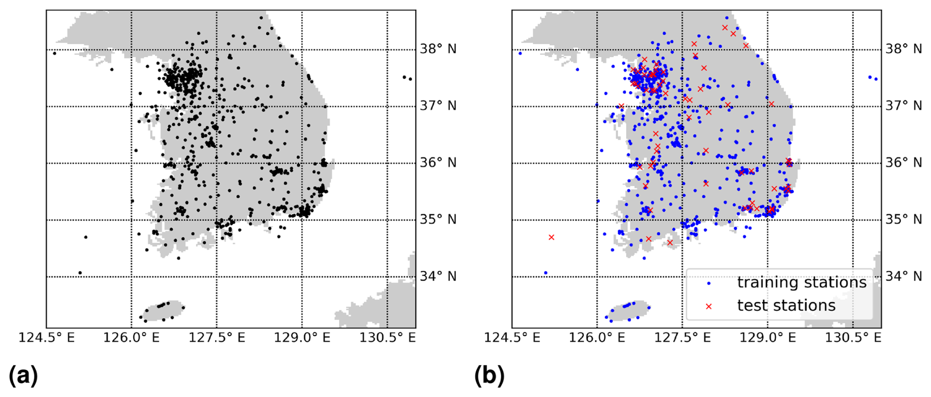
Figure 1 (a) Map with the 637 in situ stations from the air quality network of South Korea used in this study. (b) An exemplary split into 90 % training stations and 10 % test stations, considered during multiple 10-fold spatial cross-validations.

2.2 Pairing of data sources and data preprocessing

In the following, we explain the spatial and temporal pairing of the data sources. Tropospheric NO₂ VCDs and meteorological data possess spatial resolutions, as described in the previous section. Consequently, each data point covers an area (pixel) on the Earth's surface, rather than a single point. Here, we associated the location of an in situ station with the VCD pixel or meteorological pixel, whose center is nearest to the station's location (longitude, latitude). Note that the center of a VCD pixel coincides with the respective center of the GEMS satellite pixel, since no regridding is applied.

Tropospheric NO₂ VCDs are based on GEMS observations that have been collected within 30 min starting at a quarter to the respective hour, e.g., from 01:45 to 02:15 UTC. In situ measurements of surface NO₂ are available as hourly averages, starting on the hour. Temporally, we matched them with the VCDs using this timestamp and found that these data pairs showed the highest Pearson correlation. For example, VCDs between 01:45 and 02:15 UTC were matched with in situ measurements with a timestamp of 01:00 UTC. Unfortunately, at the end of our project, we learned that this was a misinterpretation of the in situ measuring times by 1 h, as the hourly averages actually start at the hour before the given timestamp instead of at the hour of the timestamp, as we had assumed. This means that the VCDs and surface NO₂ were not optimally matched within our experiments. However, the abovementioned correlation tests give us confidence that the conclusions of this study are not affected by this mistake, in particular with respect to the improvements in performance when adding data from other measurement times. To maintain consistency in notation, we continue to use the originally interpreted in situ measuring times, but they should be regarded as occurring 1 h earlier. Most meteorological features are given on the hour, which means at a specific point in time. There is one exception, namely evaporation, which is available as an hourly average starting on the hour, similar to in situ measurements. Since the averages of these data sources are taken over different periods of time, there is not a unique way to pair them temporally. Our approach is the following.

Due to the hourly resolution of all data sources, time t is expressed by t = YYYY/MM/DD/HH throughout this work. For example, t = 2021/01/23/01 refers to 23 January 2021 at 01:00 UTC. We associate the in situ measurements of surface NO₂, which started at time t and went on for 1 h, with t. In the example, time t = 2021/01/23/01 refers to surface NO₂ that has been averaged from 01:00 UTC until 02:00 UTC. Regarding tropospheric NO₂ VCDs, the same t refers to measurements that started 45 min later. Hence, t = 2021/01/23/01 describes the VCDs at a time between 01:45 and 02:15 UTC. Finally, for the meteorological features that are instantaneously on the hour, t stands for the feature's value 1 h later at t + 1. Thereby, it is closest to the corresponding VCD time frame. For example, t = 2021/01/23/01 is associated with the meteorological feature at 02:00 UTC.

To sum up, given a location z of an in situ station and a time t = YYYY/MM/DD/HH, we specified a single data point $\left(f\right(z,t),s(z,t\left)\right)$ that stores surface NO₂ s(z,t) combined with the vector of input features f(z,t), which consists of tropospheric NO₂ VCDs and meteorological features. As a data preprocessing step, we exclude data points that violate any of the following conditions:

• 1.

  All features are available at location z and time t (tropospheric NO₂ VCDs and surface NO₂ might be missing for a given z,t, for example, due to clouds).

• 2.

  Tropospheric NO₂ VCDs are non-negative. Negative VCDs can occur as a result of measurement noise in the satellite data or uncertainties in the stratospheric correction. We excluded them in an effort to improve the quality of the dataset. However, toward the end of the project, we tested the effect of this filter on a subset of the dataset and found only very small changes. This is probably due to the fact that applying this filter only leads to a reduction in the dataset by less than 0.5 %. Since negative VCDs are usually found over regions with low tropospheric NO₂ VCDs, the filter leads to a loss of the input variable and thus a loss of predictions for these regions. In retrospect, we can conclude that the implementation of this filter was not necessary, as it only had little influence on our dataset and can thus be neglected in future work. Regarding the random forests used in this study, which are trained on non-negative VCDs only, they are still able to make reasonable but potentially biased predictions over clean regions with negative VCDs as inputs. In this case, the random forests would treat negative VCDs as being zero. In contrast to the VCDs, the in situ measurements of surface NO₂ are never negative.

• 3.

  The GEMS qa value is equal to 1. Therefore, the trained models presumably cannot make reliable predictions for scenarios where the qa value is smaller than 1. It would be an interesting future direction to examine the effects of lowering the threshold for the qa value. This would result in a larger but more complex dataset.

Data points $\left(f\right(z,t),s(z,t\left)\right)$ that fulfill these conditions are collected within the so-called data basis. A data point in the data basis is not time contiguous, as it only provides information at a single time t and not at previous hours. The construction of time-contiguous datasets is described in the next section.

2.3 Description of time-contiguous datasets

In the Introduction, we motivate the use of time-contiguous inputs for machine learning models in order to predict surface NO₂. For better clarity, we introduce notations and definitions in a mathematical form.

2.3.1 Spatial and temporal coordinates

Z is the set of positions (longitude, latitude) on the Earth's surface in terms of longitude and latitude. Hence, it can be seen as the Cartesian product $[-\mathrm{180},\mathrm{180})\times [-\mathrm{90},\mathrm{90})$. In this study, we deal with in situ stations in South Korea which are located within $[\mathrm{124},\mathrm{131})\times [\mathrm{33},\mathrm{39})$; see Fig. 1a. These stations are simply identified with their location z∈Z in what follows.

T is the set of all measuring times YYYY/MM/DD/HH between January 2021 and November 2022. For example, 2021/01/23/01 refers to 23 January 2021 at 01:00 UTC. Note that for a given t ∈ T, the expression t − j for j ∈ ℕ stands for the time j hours before t. For example, for t = 2021/01/23/01 and j = 3, it is t − j = 2021/01/22/22.

2.3.2 Surface NO₂ and input features

Recall from the previous section that surface NO₂ measured at time t ∈ T and at in situ station z ∈ Z is denoted by s(z,t). As already mentioned, surface NO₂ is to be predicted from the tropospheric NO₂ VCD and meteorological variables such as the boundary layer height. These input features at z ∈ Z and t ∈ T are denoted by $f_{\mathrm{1}}(z,t),\mathrm{\dots },f_p(z,t)$, where p ∈ ℕ is the number of considered features (determined by some feature selection procedure; see Sect. 3.1). At this point, it is only important that f₁ denotes the VCDs. For simplicity, we just write $f(z,t)\in {\mathbb{R}}^p$ for the vector of all features at location z and time t.

2.3.3 Data preprocessing

We review the data preprocessing described in the previous section in light of the mathematical notation. A measurement f₁(z,t) of a tropospheric NO₂ VCD is valid if it exists (measurements may be missing at some times t ∈ T), if f₁(z,t) ≥ 0, and further if the GEMS qa value is equal to 1. For all other features $f_{\mathrm{2}}(z,t),\mathrm{\dots },f_p(z,t)$ and surface NO₂ s(z,t), it suffices that the measurement exists in order to be categorized as valid. Note again that in situ measurements of surface NO₂ are always non-negative in the present dataset.

In the following, we collect all locations and times (z,t) at which we have access to valid measurements. Namely, the domain of valid measurements Ω is defined as

$$\begin{array}{}\text{(1)}& \mathrm{\Omega }=\mathit{\left\{}\right(z,t)\in Z\times T:\text{and}s(z,t),f_{\mathrm{1}}(z,t),\mathrm{\dots },f_p(z,t\left)\text{are valid}\mathit{\right\}}.\end{array}$$

2.3.4 Time-contiguous datasets

In order to consider time-contiguous measurements, we define for N ∈ ℕ the set

$$\begin{array}{}\text{(2)}& {\mathrm{\Omega }}_N=\mathit{\left\{}\right(z,t)\in \mathrm{\Omega }:(z,t-j)\in \mathrm{\Omega }\text{for}j=\mathrm{1},\mathrm{\dots },N-\mathrm{1}\mathit{\}}.\end{array}$$

In other words, Ω_N collects locations and times (z,t) at which valid measurements also exist for at least N − 1 previous hours. Note that ${\mathrm{\Omega }}_N\subseteq {\mathrm{\Omega }}_{N-\mathrm{1}}\subseteq \mathrm{\Omega }$ for all N ∈ ℕ, and Ω₁ coincides with Ω, the domain of valid measurements. Given (z,t) ∈ Ω_N and $k\in \mathit{\{}\mathrm{1},\mathrm{\dots },N\mathit{\}}$, this definition allows us to build a valid time-contiguous feature vector:

$$\begin{array}{}\text{(3)}& \left(\begin{array}{c}f(z,t)\\ f(z,t-\mathrm{1})\\ \mathrm{⋮}\\ f(z,t-k+\mathrm{1})\end{array}\right)\in {\mathbb{R}}^{pk},\end{array}$$

which can serve as input for a machine learning model ${\mathit{\phi }}_{\mathit{\theta }}:{\mathbb{R}}^{pk}\to \mathbb{R}$ to predict surface NO₂ s(z,t).

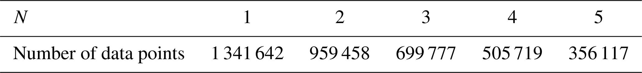
Hence, Ω_N parameterizes the datasets occurring in our study. In fact, Ω_N parameterizes N different datasets of feature vectors paired with surface NO₂. They only differ within the time contiguity $k\in \mathit{\{}\mathrm{1},\mathrm{\dots },N\mathit{\}}$ of the feature vectors, that is, how many previous hours (namely k − 1) are considered for each feature (at most N − 1). Mathematically, these N datasets can be understood as functions $D_{N,k}:{\mathrm{\Omega }}_N\to {\mathbb{R}}^{pk}\times \mathbb{R}$ mapping $(z,t)\in {\mathrm{\Omega }}_N$ to the feature vector in Eq. (3) paired with surface NO₂ at location z and measuring time t. Further, D_1,1 just describes the data basis mentioned in the previous section.

The number of elements in Ω_N – that is, the size of all datasets D_N,k – are listed in Table 1 for $N=\mathrm{1},\mathrm{\dots },\mathrm{5}$. Hence, if a model is to be trained with time-contiguous inputs (k>1), this comes with the price of a smaller number of data points. For example, time-contiguous models cannot be used to make predictions at initial hours of a day. It should be mentioned that among all features described in the previous section, ERA5's soil type and high vegetation cover are the only features that do not depend on time t. This is why, in practice, we never included them k times but rather a single time only, when building the time-contiguous feature vector in Eq. (3) at (z,t). However, for the sake of simplicity, we neglect this fact within the notation.

Table 1 Size of time-contiguous datasets D_N,k, which consist of data points for which valid measurements also exist for at least N − 1 previous hours, but only k values are used for constructing the time-contiguous feature vector in Eq. (3). Note that the size is independent of the time contiguity k. The overall considered time period covers January 2021 until November 2022.

2.3.5 Normalization of input features

For any given split into training and test data, the input features are normalized before being fed into the machine learning models to improve the stability of their performance. More precisely, each feature undergoes an affine transformation A such that its mean on the training data becomes 0 and its standard deviation becomes 1. Let ${\stackrel{\mathrm{‾}}{x}}_{\mathrm{train}}$ and σ_train be the mean and standard deviation of a feature in the training data, respectively. Then, the transformation applied to both training and test data points is given by

$$\begin{array}{}\text{(4)}& A\left(x\right)={\displaystyle \frac{x-{\stackrel{\mathrm{‾}}{x}}_{\mathrm{train}}}{{\mathit{\sigma }}_{\mathrm{train}}}}\end{array}$$

and is applied to both training and test data points.

A compact overview of the spatial and temporal resolutions of the data sources used is shown in Table 2. In addition, for each data source, the applied data preprocessing steps are listed. Moreover, the overall workflow for all data-processing steps is illustrated in the flowchart in Fig. 2.

Table 2 Overview of spatial and temporal resolutions of the data sources used. Applied preprocessing steps are also listed for each data source.

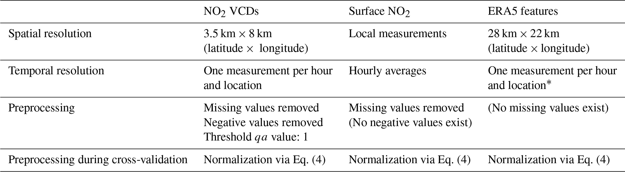
^* Exception: ERA5 evaporation is available as hourly averages.

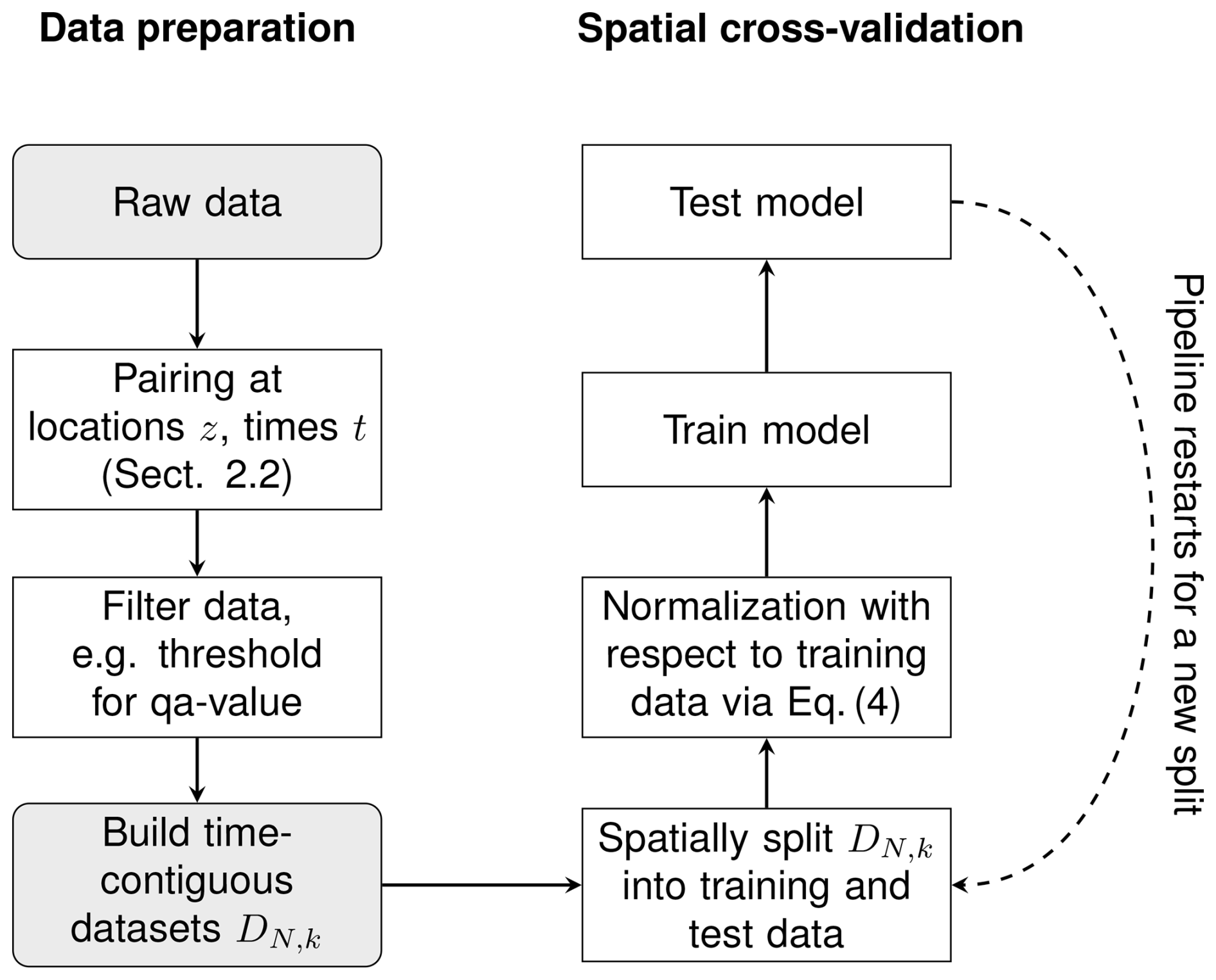
Figure 2 A flowchart for all data processing steps. The left column shows the construction of the time-contiguous datasets D_N,k. For preprocessing, the data are filtered according to the criteria in Sect. 2.2; see also Table 2. Evaluating the performance of models on D_N,k is done via spatial cross-validation; see Sect. 3.2. This pipeline is outlined in the right column.

3 Experimental setup

In Sect. 3.2, we describe and discuss the experiments conducted to inspect our main research questions. Before that, we explain how features were selected for these experiments. Afterwards, we discuss different performance measures and loss functions used to evaluate the quality of the models' prediction of surface NO₂ on test data points.

3.1 Feature selection

In this study, we considered 23 different features from which we selected 17 to build the feature vectors used in Eq. (3) as inputs for the machine learning models. The selected and excluded features are listed in Table B1 and are used in Experiment 1 and Experiment 2; see Sect. 3.2. For the feature selection, we proceeded as follows: on the data basis D_1,1, we considered 200 different splits into 90 % training and 10 % test stations. For the training data of each split, we calculated the Pearson correlation (see Sect. 3.3 for a definition) between in situ measurements of surface NO₂ and the respective feature. We selected features which had an absolute mean correlation larger than 0.1. It is worth mentioning that for all 17 of the aforementioned features, the correlation was in fact larger than 0.1 in 98 % of the splits, whereas this was never the case for the remaining six features. More complex feature selection strategies could be applied in the future. However, during this study we focus on the benefits of time-contiguous inputs and not on the optimal choice of input features.

3.2 Experiments

Recall from Sect. 2.3 that Ω_N is the set of locations and measuring times (z,t) at which all measurements are also available at (N−1) previous hours. Note that Ω_N does not parameterize a single dataset but N different datasets $D_{N,k}:{\mathrm{\Omega }}_N\to {\mathbb{R}}^{pk}\times \mathbb{R}$ via

$$D_{N,k}:(z,t)⟼\left(\left(\begin{array}{c}f(z,t)\\ f(z,t-\mathrm{1})\\ \mathrm{⋮}\\ f(z,t-k+\mathrm{1})\end{array}\right),s(z,t)\right),$$

which only differ in the time contiguity $k\in \mathit{\{}\mathrm{1},\mathrm{2},\mathrm{\dots },N\mathit{\}}$ of the time-contiguous feature vector $\left(f\right(z,t),\mathrm{\dots },f(z,t-k+\mathrm{1}){)}^T$, defined in Eq. (3).

As mentioned in the Introduction, we wish to inspect how well a machine learning model is able to make predictions of surface NO₂ at locations from which it has not seen training data. This is why we use multiple (six-times) 10-fold spatial cross-validations in all experiments. This involves splitting the dataset 60 times randomly into 90 % training and 10 % test data based on the locations of the in situ stations; see Fig. 1b for a visualization of a single split. Performance is measured on all the different test datasets and averaged. Due to the limited number of available in situ stations, significant variance in the model's performance is expected across different splits. Therefore, multiple 10-fold spatial cross-validations provide a more reliable estimate of the model's performance compared to a single 10-fold spatial cross-validation. In all that follows, whenever it is mentioned that a machine learning model is trained or tested on D_N,k, it implies that the model is trained or tested solely on those data points in D_N,k corresponding to the designated training or test stations. Note that for fixed N, surface NO₂ that is to be predicted in D_N,k is exactly the same for all the different k. Furthermore, for all models, the same 60 splits into training and test stations are considered for spatial cross-validation, which ensures perfect comparability. For a basic outline of a cross-validation pipeline, see Fig. 2.

Let us recall from Sect. 1.1 that our main research question is whether time-contiguous inputs for machine learning models enable higher accuracy for predicting surface NO₂. We propose two experiments to gain insight into this question.

•  

  Experiment 1. Do time-contiguous input features provide additional information?
  

  For fixed N, consider the datasets D_N,k for different time-contiguities k = $\mathrm{1},\mathrm{\dots },N$. The chosen machine learning model, such as a random forest regressor, is trained and tested on D_N,k for all 60 splits from spatial cross-validation. A comparison is made with respect to different k. Fixing N ensures that, regardless of k, the same ground truth (surface NO₂) is predicted for computing the cross-validation scores on the test sets. Additionally, all models are trained with the same number of training data points, eliminating any advantage or disadvantage due to differing dataset sizes. Thus, this experiment provides pure insights into the information gain provided by time-contiguous inputs. We conduct this experiment for all $N\in \mathit{\{}\mathrm{2},\mathrm{3},\mathrm{4},\mathrm{5}\mathit{\}}$.

•  

  Experiment 2. Are time-contiguous input features beneficial in spite of a smaller available dataset?
  

  In the first experiment, the models were trained on the same amount of training data, with the time contiguity k being the only variable. However, for smaller k there is much more data available that can be used for training the respective models; see Table 1. Therefore, we need to extend the first experiment as follows: we still test performance on D_N,k for a fixed N. But for different k, we train models on D_M,k for all $M\in \mathit{\{}k,k+\mathrm{1},\mathrm{\dots },\mathrm{5}\mathit{\}}$, i.e., with a different amount of training data. Note that in Experiment 1, M has always been set to N. These additional investigations are crucial to evaluate whether time-contiguous inputs are beneficial for predicting surface NO₂. Even if time-contiguous inputs provide additional information (as seen in the first experiment), why should one use them if training with less or even no time contiguity on larger datasets yielded better results? Again, we conduct this experiment for all $N\in \mathit{\{}\mathrm{2},\mathrm{3},\mathrm{4},\mathrm{5}\mathit{\}}$, where N determines the test datasets.

In a third experiment, we analyze the influence of some features on the performance of the machine learning models. Since testing all the different combinations of input features for all 15 different training and test cases in Experiment 2 would be out of the scope of this study, we focus only on the influence of the tropospheric NO₂ VCDs, surface height, and latitude. Note that longitude has not been included during feature selection due to a low correlation with surface NO₂. Tropospheric NO₂ VCDs are the main consideration within this third experiment since they represent the feature which shows, among all considered input features, by far the best Pearson correlation with surface measurements of NO₂, namely around 0.626; see also Table B1. Although latitude only has a small variation over South Korea and hence a presumably small impact on predicting surface NO₂, we considered it (and also longitude) during feature selection to check whether it provides some helpful information. Other studies have also used spatial coordinates to predict surface NO₂, mainly over large regions (Ghahremanloo et al., 2021; Li et al., 2022; Qin et al., 2020) but also over smaller regions, such as over Switzerland (de Hoogh et al., 2019). Using spatial coordinates as inputs for a model, however, carries the risk of spatial overfitting, which could make it more difficult to predict surface NO₂ outside of South Korea with the same model. This is why we inspect whether the models perform equally well over South Korea without having latitude and surface height as inputs.

•  

  Experiment 3. What is the influence of tropospheric NO₂ VCDs, latitude, and surface height on the performance?
  

  We compare four different settings of input features:

  •  

    Setting 1. All features selected in Sect. 3.1 are included, which is exactly the same setup as for Experiments 1 and 2.

  •  

    Setting 2. VCDs are excluded as an input feature.

  •  

    Setting 3. Latitude and surface height are excluded.

  •  

    Setting 4. VCDs, latitude, and surface height are excluded.

  We also conduct Experiment 2 for Settings 2, 3, and 4 and draw a comparison between these settings regarding different performance measures. Further, within these four settings, we inspect the models' ability and reliability in achieving performance gains when including time-contiguous input features.

3.3 Performance measures

Throughout this section, x^† ∈ ℝⁿ is a vector consisting of n in situ observations of surface NO₂, where each coefficient $x_i^{†}(t_i,z_i)=s(t_i,z_i)$ corresponds to a measurement that has been taken at a given time t_i and location (longitude, latitude) z_i of a given in situ station. For the sake of simpler notation, we just write $x_i^{†}$, neglecting the dependence on t_i and z_i within the notation. Similarly, x∈ℝⁿ denotes the predictions for x^† made by a machine learning model, such as linear regression or random forests. In the following, we discuss different performance measures that quantify the gap between the model's prediction x for x^†, the observed surface concentration of NO₂.

As pointed out in the Introduction, spatial cross-validation is considered within this research; i.e., data are split into training and test data station-wise. Since the overall number of in situ stations is relatively small, namely 637, the statistical properties of surface NO₂ for different test sets are very likely to differ. In particular, the mean or standard deviation of surface NO₂ of different test sets will vary. Hence, in order to compare the quality of surface NO₂ predictions on different test sets, it is reasonable to use error measures that are more robust or even insensitive to different data distributions.

In order to ensure better comparability of performances of a model on different test sets, one should not use absolute performance measures such as the mean absolute error or root mean square error, since they depend on the scale of the different test sets.

At first glance, it seems reasonable to consider the mean percentage error:

$$\text{MPE}\left(x^{†},x\right)=\sum _{i=\mathrm{1}}^n{\displaystyle \frac{\mathrm{|}{x}_i^{†}-x_i\mathrm{|}}{\mathrm{|}{x}_i^{†}\mathrm{|}}}.$$

The reason why the mean percentage error enables us to compare performances on different test sets is the following property: for every c∈ℝⁿ with c_i≠0 it holds that

$$\text{MPE}\left(c{x}^{†},cx\right)=\text{MPE}\left(x^{†},x\right),$$

where cx^† denotes pointwise multiplication. However, since many in situ measurements $x_i^{†}$ are very close to or equal to zero, the mean percentage error becomes unstable. As a trade-off, we consider performance measures $E\left(x^{†},x\right)$ that are scale-insensitive; i.e., for every $\mathit{\lambda }\in \mathbb{R}\setminus \mathit{\left\{}\mathrm{0}\mathit{\right\}}$ it holds that

$$E\left(\mathit{\lambda }{x}^{†},\mathit{\lambda }x\right)=E\left(x^{†},x\right).$$

The normalized mean absolute error (NMAE) can be written as

$$\text{NMAE}\left(x^{†},x\right)={\displaystyle \frac{\sum _{i=\mathrm{1}}^n\mathrm{|}{x}_i^{†}-x_i\mathrm{|}}{\sum _{i=\mathrm{1}}^n\mathrm{|}{x}_i^{†}\mathrm{|}}},$$

so the NMAE is just the mean absolute error divided by the mean absolute value of the ground truth x^†. If normalization by the standard deviation of x^† instead of its mean were considered, this would lead to a measure similar to the coefficient of determination R²; see Appendix A. Note that in contrast to the mean absolute error, NMAE is scale-insensitive. Similarly, we define the normalized mean square error (NMSE) as

$$\text{NMSE}\left(x^{†},x\right)={\displaystyle \frac{\sum _{i=\mathrm{1}}^n\mathrm{|}{x}_i^{†}-x_i{\mathrm{|}}^{\mathrm{2}}}{\sum _{i=\mathrm{1}}^n\mathrm{|}{x}_i^{†}{\mathrm{|}}^{\mathrm{2}}}}.$$

Whenever we talk about the correlation between x^† and x, we mean the Pearson correlation coefficient (C), which is defined as

$$C\left(x^{†},x\right)={\displaystyle \frac{\text{cov}\left(x^{†},x\right)}{\mathit{\sigma }\left(x^{†}\right)\mathit{\sigma }\left(x\right)}},$$

where $\text{cov}\left(x^{†},x\right)$ denotes the covariance between x^† and x and σ(x^†), and σ(x) is the standard deviation of x^† and x, respectively. It should be noted that this is not a performance measure in the sense that x^† = x if and only if $C\left(x^{†},x\right)$ = 1. Nevertheless, it quantifies the linear relationship between x and x^†. Furthermore, it is frequently used in the literature, which is the reason why we consider it in our work, too.

We considered two further scale-insensitive performance measures, the coefficient of determination (R²) and the index of agreement (IOA), which are defined in Appendix A.

4 Machine learning models considered

As mentioned in the Introduction, numerous machine learning models have been considered for predicting surface NO₂ in the literature. Examining the benefit of time-contiguous input features for all the different models is beyond the scope of this research. This is because fair comparisons require individual hyperparameter tuning for the models, with different time contiguities of the input features. Therefore, we restrict our attention to one approach that, on the one hand, has performed well in the literature and, on the other hand, does not have many hyperparameters to tune. If there were many hyperparameters to be tuned and the models' performance were very sensitive to the choice of these hyperparameters, there would be a risk that better performance was achieved only due to better hyperparameter tuning. In this study, we use a random forest regressor, which we describe in Sect. 4.2, and present the selected hyperparameters. As a reference, we consider a simple linear regression approach, which we recap first in the next section. At the outset of this study, we also experimented with neural networks (NNs) to estimate surface NO₂. While we observed similar results to those obtained with random forests, the training time for NNs was considerably longer. Therefore, and due to the large number of hyperparameters and architectural design choices for NNs, conducting as many experiments with NNs as we did with random forests would have been outside the scope of our study. This is why we chose to focus on random forests, but we expect similar performance gains for neural networks as well.

4.1 Linear regression

Although it has already been shown, e.g., by Ghahremanloo et al. (2021), that linear regression models are not the best for predicting surface NO₂, we consider an ordinary least squared regressor as a reference in our study, mainly because it has no tunable hyperparameters, such as regularization parameters, or architecture parameters like those in neural networks (e.g., number of layers, width of layers, activation functions, skip connections). Thus, it provides a clear view on the question of whether time-contiguous inputs are beneficial for this linear regression model. During this study, we used the ordinary least squares regression model provided by the Python scikit-learn package (version 1.2.2, Pedregosa et al., 2011). In our case of predicting surface NO₂ from time-contiguous inputs, the linear regression model is a parameterized function

$$\begin{array}{c}{\displaystyle }{\mathit{\phi }}_{\mathit{\theta }}:{\mathbb{R}}^{pk}⟶\mathbb{R}\\ {\displaystyle }y⟼Ay+b,\end{array}$$

where y = $\left(f\right(z,t),\mathrm{\dots }f(z,t-k+\mathrm{1}){)}^T$ is a (time-contiguous) feature vector defined in Eq. (3), A is a 1×pk matrix, and b∈ℝ is a bias term. Let $(y_n,s_n{)}_{n=\mathrm{1}}^N$ be training data, where y_n is a feature vector at location z_n and time t_n and s_n the corresponding in situ measurement of surface NO₂ at time t_n. Training φ_θ then means to search for a parameter θ = (A,b) that solves the following minimization problem:

$$\underset{\mathit{\theta }}{min}\sum _n\mathrm{|}{\mathit{\phi }}_{\mathit{\theta }}\left(y_n\right)-s_n{\mathrm{|}}^{\mathrm{2}}.$$

We choose to minimize the squared error since the computation time is much shorter compared to that of other losses such as the absolute error.

4.2 Random forests

There are two main reasons why random forests, a machine learning model originally proposed by Breiman (2001), are considered within this research. First, they have already proven to be powerful for predicting surface NO₂ in various studies; see, for example, Di et al. (2020), Ghahremanloo et al. (2021), Li et al. (2022), and Huang et al. (2023) on OMI and TROPOMI data and Yang et al. (2023b) on GEMS data. Second, the studies of Probst et al. (2018, 2019) suggest that random forests are less tunable compared to other machine learning approaches. “Tunable” is defined as the extent to which the performance of a random forest with typical default hyperparameters can be enhanced by adjusting (tuning) those hyperparameters. As discussed before, this reduces the risk of drawing incorrect conclusions about the benefit of using time-contiguous inputs.

In fact, according to Probst et al. (2018), there are mainly four hyperparameters that empirically determine the performance of a random forest:

• The first hyperparameter is the number of randomly drawn features considered at every split of a tree. In the Python scikit-learn software package (version 1.2.2, Pedregosa et al., 2011) that we use for this study, it is called max_features. However, in several other software packages, it is denoted as mtry.

• The second hyperparameter is the number of trees that make up the random forest. In scikit-learn it is called n_estimators. To be precise, it is not actually a hyperparameter, since more trees are in general more advantageous; see, e.g., Genuer et al. (2008) or Scornet (2017).

• The third hyperparameter is the maximal number of (randomly drawn) data samples from the training set that is used for the construction of an individual tree, denoted as max_samples in scikit-learn.

• The fourth hyperparameter is the minimal number of observations that lands in a leaf node during the training process. In scikit-learn it is called min_samples_leaf.

In their experiments, Probst et al. (2018) observed that max_features had the biggest influence on the performance and the influence of max_samples and min_samples_leaf was smaller. This is why, during hyperparameter tuning, we mainly focus on max_features but also consider different values for max_samples. Regarding max_samples, we consider values between 50 % and 100 % of the size of the training dataset. On the other hand, for max_features, values between 1 and $\left(pk\right)/\mathrm{3}$ are considered, where pk is the number of inputs for the model, i.e., the dimension of the time-contiguous feature vector in Eq. (3). The value $\left(pk\right)/\mathrm{3}$ is the default value of scikit-learn. Genuer et al. (2008) suggested $\sqrt{pk}$ for problems in which the number of data points is much larger than the number of input features pk, which is clearly the case in our study (hundreds of thousands of data points versus less than 90 input features). As pk ≥ 17, the value $\sqrt{pk}$ is always within the considered interval during optimization. In fact, $\sqrt{pk}$ turns out to be quite close to the optimal choice in our hyperparameter study. Regarding min_samples_leaf, we inspect two typical default values, namely 1 and 5. Following the rule “the more, the better” for the number of trees (n_estimators) in the forest, we use 8000 trees while tuning the other hyperparameters. Hyperparameter selection is made according to the spatially cross-validated (10 splits) NMSE, leading to max_features = 2, 3, 3, 3, 4 for time contiguity k = 1, 2, 3, 4, 5 and further min_samples_leaf and max_samples = 5 using 100 % of the size of the training data. All remaining hyperparameters are always set to the default values within scikit-learn.

With 8000 trees, we chose a very high value for the number of trees, which may require an explanation. The good news is given first: comparable results can be obtained with far fewer trees in the forest. However, for hyperparameter tuning and to gain a clearer insight into the benefit of time-contiguous features, it is reasonable to choose a large number of trees, which we illustrate in the following: the random forest algorithm in scikit-learn is not deterministic, meaning that if the model is trained on the same training data multiple times, the trained forests will differ from each other, also causing the performance of the respective test dataset to vary. However, we observe that with a higher number of trees in the forest, the variance in the performance decreases for all considered performance measures. In Fig. C1 in Appendix C, we illustrate this effect using a single split into training and test stations. Two random forests, one with 30 trees and the other with 8000 trees, are each trained and tested 20 times on the same data, similar to Experiment 2, but with 20 repetitions of the same split instead of 60 different splits. We observe that with 30 trees the scores on the test data, such as Pearson correlation, NMSE, or NMAE, exhibit some variance. In contrast, there is barely any variance in the case of 8000 trees. This has the advantage that for each split into training and test stations, the random forest only needs to be trained once to get an interpretable result. Thereby, it also reduces the risk of choosing non-optimal hyperparameters. Therefore, during all experiments, we set the number of trees to a very large number (n_estimators = 8000) to stabilize the non-deterministic behavior of training a random forest. Note that stability can probably be achieved with far fewer than 8000 trees. However, in order to reduce the bias from the observation above for a single split and single choice of hyperparameters, we choose a very large number that is still manageable regarding storage and computation time.

5 Results

Before presenting the results and starting the discussion, it is important to recall that for a given spatial split into training and test in situ stations, training or testing a machine learning model on the dataset D_N,k means that only the data points corresponding to the training or test station locations are used, respectively. Furthermore, for fixed N, the in situ measurements s(z,t) of surface NO₂ (ground truth) that are to be predicted in D_N,k are exactly the same for all the different k. Further, recall that D_N,k can be thought of as the set of data points for which measurements at all N−1 previous hours are also guaranteed to be available, but only k − 1 values are added to the time-contiguous feature vector in Eq. (3).

In the following discussion of the experiments, introduced in Sect. 3.2, we focus exclusively on the results when D_4,k is used for constructing test datasets, i.e., for N = 4 only. This is because we observe a similar benefit from a larger time contiguity k when evaluating the machine learning models' performance on D_N,k for $N\in \mathit{\{}\mathrm{2},\mathrm{3},\mathrm{5}\mathit{\}}$. As a further example, we provide detailed results for N = 2 in Figs. C2 and C3 in Appendix C.

5.1 Experiment 1: time-contiguous inputs provide additional information

In Experiment 1, we train linear regression models and random forests on D_4,k for different time contiguities $k\in \mathit{\{}\mathrm{1},\mathrm{\dots },\mathrm{4}\mathit{\}}$ of the input features. The test performances of these models are evaluated via six-times spatial 10-fold cross-validation and are illustrated in Figs. 3b and 4b, respectively. Specifically, we show average Pearson correlation, NMSE, and NMAE over all 60 splits into training and test stations. We observe that, on average, both linear regression and random forests benefit from a larger time contiguity k regarding all considered performance measures. For example, the average correlation strictly increases from 0.702 for k = 1 to 0.737 for k = 4 in the case of linear regression, and for random forests, it increases from 0.802 to 0.817. Further, the average NMSE decreases from 0.196 to 0.171 for linear regression and from 0.139 to 0.129 for random forests. Therefore, both models benefit from larger time contiguity, but linear regression shows greater improvement, which is expected as it cannot model non-linear effects. Furthermore, we observe that the larger k, the smaller the improvement compared to the case k − 1, which is to be expected since input features at time t − k presumably have a decreasing impact on surface NO₂ at time t for larger k.

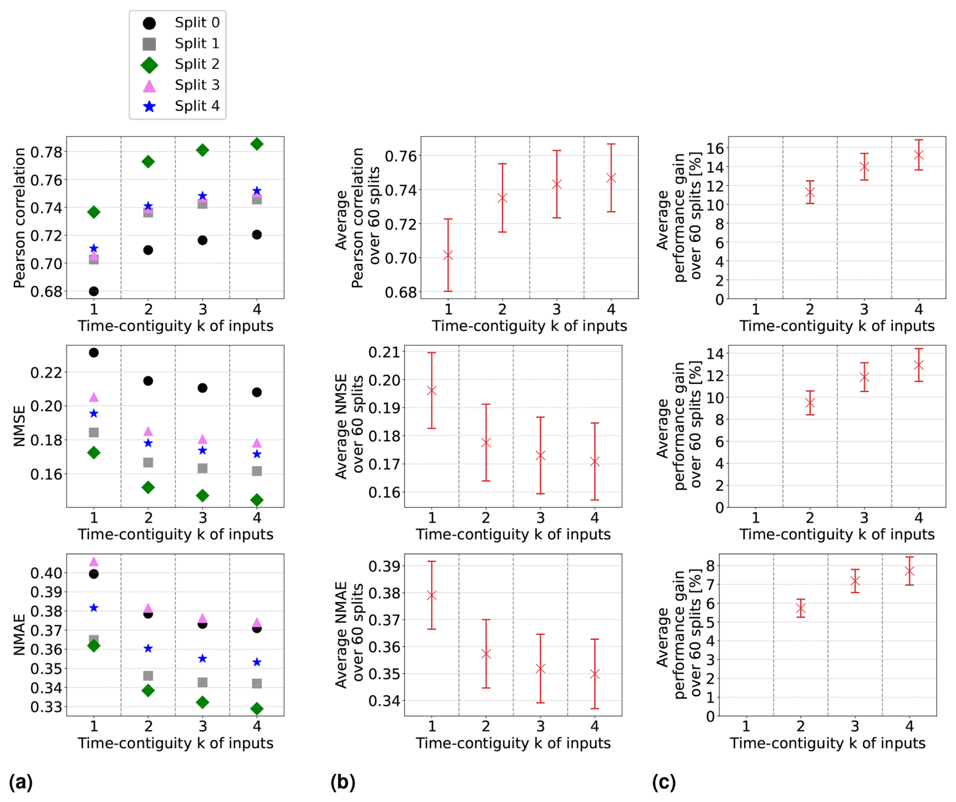
Figure 3 Linear regression models have been trained and tested on datasets D_4,k for 60 different splits into training and test stations, with different time contiguity k of the input features. In panel (a), performances on test sets are shown for five exemplary station splits with respect to three performance measures. Panel (b) shows the average performance over all 60 splits, with error bars illustrating the standard deviation. Panel (c) shows the average performance gain relative to the case k = 1; see Eq. (5) for the definition of performance gain. Across each row, the same performance measure is considered. The exact values in panel (b) can be found in Table B2, columns D_4,1 to D_4,4.

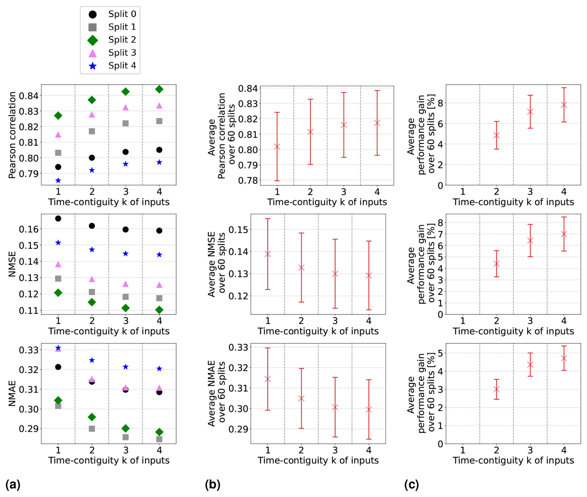
Figure 4 Same as Fig. 3 but for random forests trained and tested on datasets D_4,k for 60 different splits into training and test stations, with different time contiguity k of the input features. In panel (a), performances on test sets are shown for five exemplary station splits with respect to three performance measures. Panel (b) shows the average performance over all 60 splits, with error bars illustrating the standard deviation. Panel (c) shows the average performance gain relative to the case k = 1; see Eq. (5) for the definition of performance gain. Across each row, the same performance measure is considered. The exact values in panel (b) can be found in Table B3.

Although the visualization of average performances suggests an overall trend, it does not clearly indicate whether larger time contiguities (k > 1) consistently improve performance across all 60 station splits during cross-validation compared to k = 1. However, we found that this improvement holds true for all 60 station splits. The performance curves for individual splits are more or less parallel to the average curve. In Figs. 3a and 4a, we illustrate this for exemplary station splits, where only five splits are shown for better visibility. To quantify the gain in performance for individual splits between using time contiguity k = 1 and larger time contiguities k>1, we proceed as follows: for a given test dataset, let E_k be the test performance (e.g., correlation) achieved by the model using time contiguity k for its inputs. We define the performance gain of this model over the case with no time contiguity k = 1 in Experiment 1 as

$$\begin{array}{}\text{(5)}& {\displaystyle \frac{E_{\mathrm{1}}-E_k}{E_{\mathrm{1}}-E_{\mathrm{opt}}}},\end{array}$$

where E_opt is the optimal value of the respective performance measure; e.g., E_opt = 1 for the Pearson correlation or E_opt = 0 for NMSE and NMAE. The average performance gains for the cases $k\in \mathit{\{}\mathrm{2},\mathrm{3},\mathrm{4}\mathit{\}}$ compared to k = 1 are depicted in Figs. 3c and 4c for linear regression and random forests, respectively. In both cases and for all performance measures, the highest average performance gain is achieved with k = 4. Specifically, linear regression models achieve average performance gains of 15.2 % in correlation, 13.0 % in NMSE, and 7.7 % in NMAE, whereas random forests achieve gains of around 7.8 %, 7.0 %, and 4.7 %, respectively. It is noteworthy that, for linear regression, the performance gain across all 60 splits is approximately at least 12.0 % in correlation, 10.0 % in NMSE, and 6.1 % in NMAE. On the other hand, random forests achieve performance gains of at least 4.6 %, 4.0 %, and 3.1 %, respectively. Therefore, utilizing a larger time contiguity consistently provided beneficial additional information for both linear regression and random forest models.

Additionally, for k = 1 and the best time contiguity k = 4, we examine for each split the orthogonal regression curve between the models' predictions and ground truth measurements of surface NO₂ on the corresponding test dataset. For a fixed split, this is illustrated as a two-dimensional histogram in the first row of Fig. 5 for linear regression and in Fig. 6 for random forests. Although the histograms are restricted to surface NO₂ and predictions between 0 and 40 µg m⁻³ for better visibility, all data points are taken into account to determine the orthogonal regression curve. It becomes evident that both the slope and the bias of the orthogonal regression curve improve for k = 4 (panel b) compared to k = 1 (panel a), where improvement means that the slope becomes closer to 1 and the bias closer to 0. In the second row of these figures, we plot the mean orthogonal regression curve, which represents the mean slope and mean bias of all 60 orthogonal regression curves. An upper bound for all these curves is represented by the line with the maximal slope and bias across all splits (note that maximal slope and bias might not occur for the same split). Similarly, a lower bound is obtained, and both bounds are shown within the same plots. Both the mean orthogonal regression curve and the upper and lower bounds improved for k = 4 for both linear regression and random forests. However, the improvement is larger for the linear regression models, which is consistent with the previous discussion on performance measures, such as NMSE.

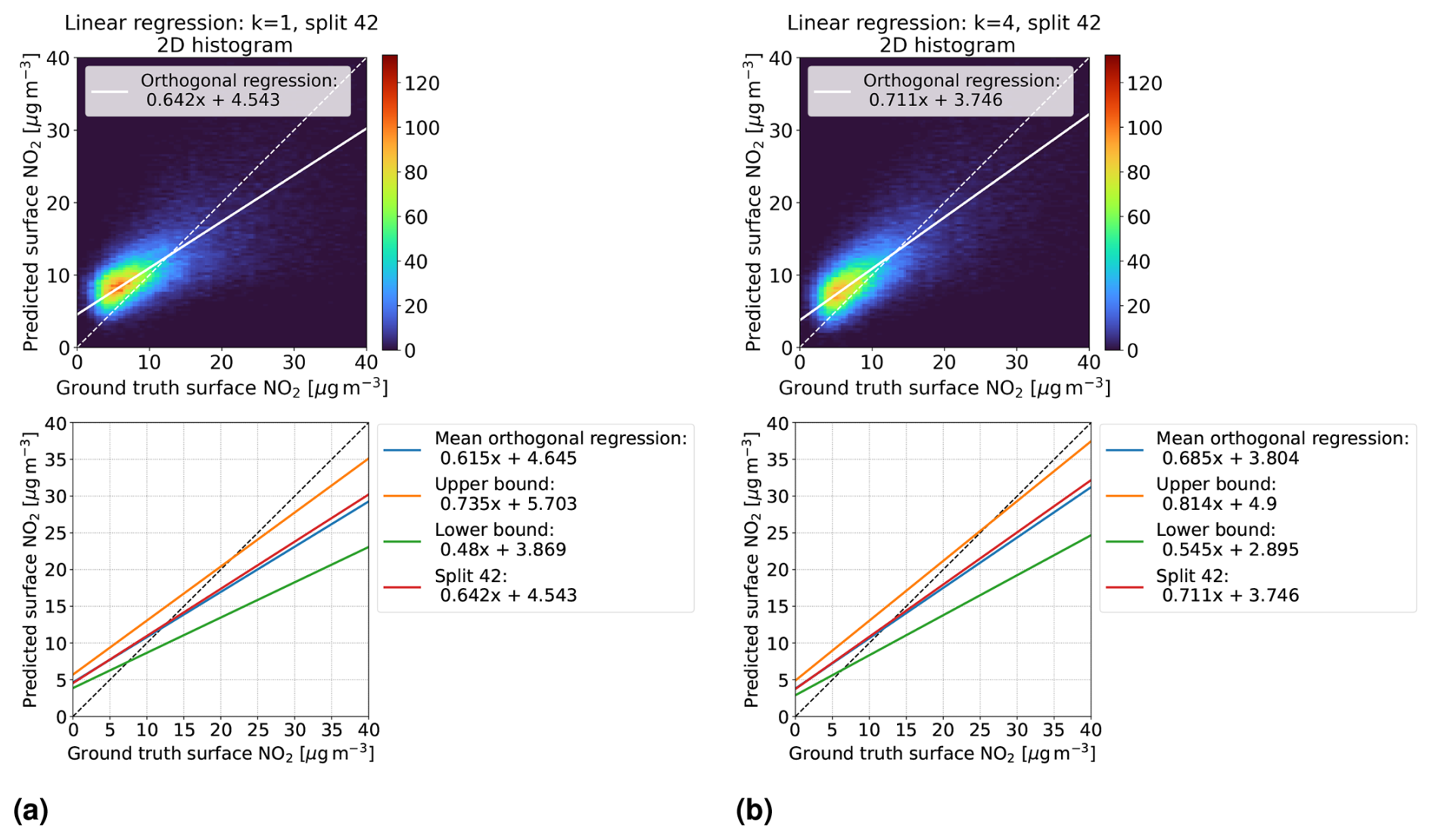
Figure 5 Linear regression models trained on D_4,k with time contiguities (a) k = 1 and (b) k = 4. First row: for a fixed split (number 42) into training and test stations, the models' predictions on the corresponding test set D_4,k are compared with in situ measurements of surface NO₂ (ground truth) in a two-dimensional histogram. Second row: for all 60 station splits, orthogonal regression is considered between predicted and ground truth surface NO₂. Mean orthogonal regression refers to the line of average slope and bias over all 60 regression lines (blue line). The regression line for the example in the first row is also shown (red line).

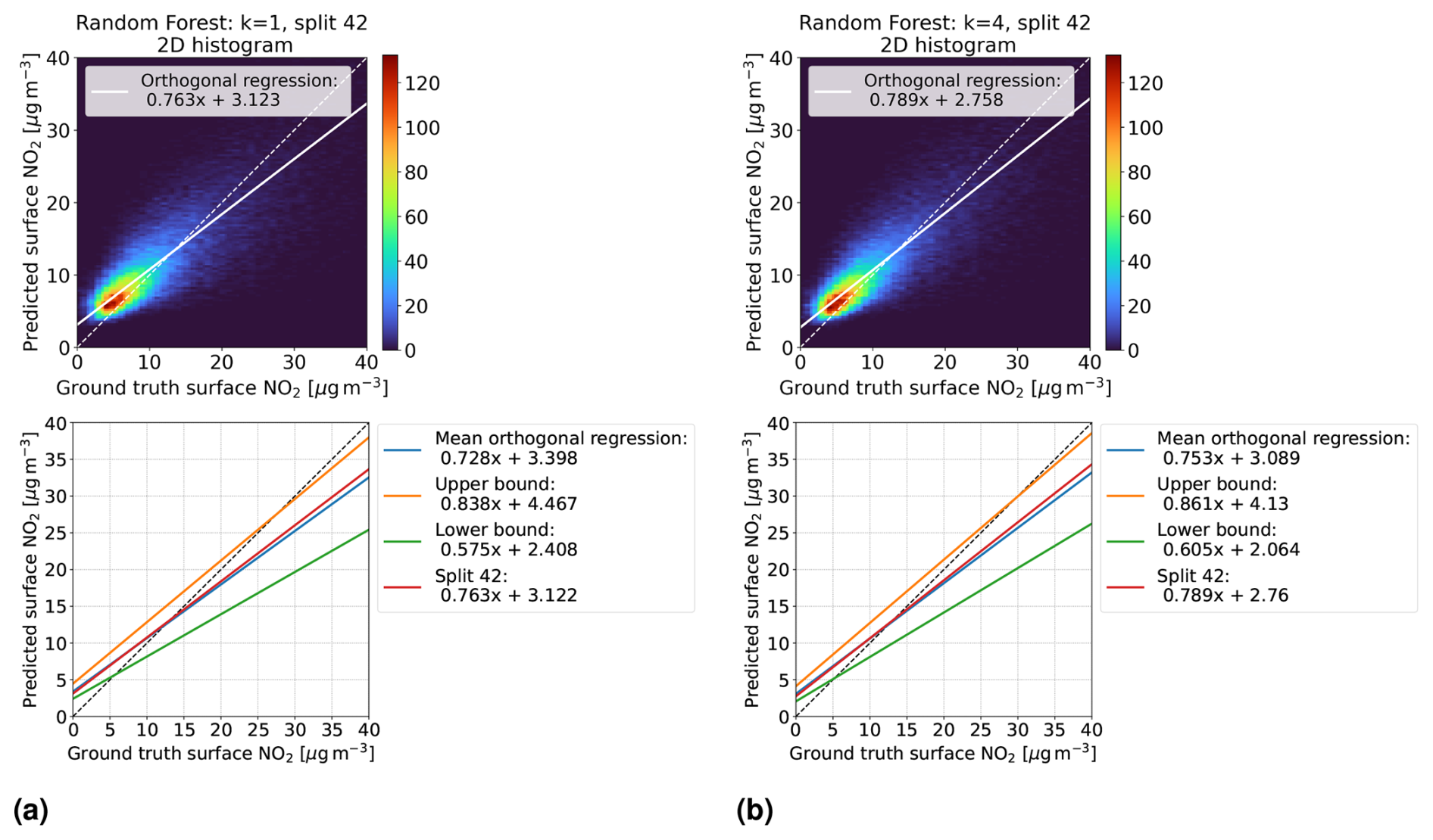
Figure 6 Same as Fig. 5 but for random forests trained on D_4,k with time contiguities (a) k = 1 and (b) k = 4. First row: for a fixed split (number 42) into training and test stations, the models' predictions on the corresponding test set D_4,k are compared with in situ measurements of surface NO₂ (ground truth) in a two-dimensional histogram. Second row: for all 60 station splits, orthogonal regression is considered between predicted and ground truth surface NO₂. Mean orthogonal regression refers to the line of average slope and bias over all 60 regression lines (blue line). The regression line for the example in the first row is also shown (red line).

We want to stress another observation: looking at the upper and lower bounds of the orthogonal regression curves, we see that all slopes are smaller than 1, whereas all biases are positive. Further, there is a noticeable gap towards the identity line. Regarding the latter, one possible explanation could be that spatially splitting the dataset into training and test sets causes a large difference in the statistical properties of the training and test sets. This may simply be because there are overall just 637 different in situ stations available, so the law of large numbers may not yet apply well when sampling 10 % of test stations. However, this does not explain why the slopes and biases are not more symmetrically distributed around slope 1 and bias 0. Studying the impact of the number of available in situ stations and their locations on the slopes and biases of these orthogonal regression curves will be an interesting task for future work.

5.2 Experiment 2: time-contiguous inputs are beneficial in spite of a smaller dataset

In Experiment 1, the models were trained and tested on D_N,k for fixed N but with a different time contiguity $k\in \mathit{\{}\mathrm{1},\mathrm{\dots },N\mathit{\}}$ of their input features. This means that for a fixed station split, the number of training data points was the same for all the different k, since the size of D_N,k only depends on N (see Table 1). However, for $M\in \mathit{\{}k,\mathrm{\dots },N-\mathrm{1}\mathit{\}}$, there would be significantly more data points available in D_M,k than in D_N,k, which could be used during training. To make a fair conclusion about whether a larger time contiguity (k > 1) in the models' input is more beneficial compared to time contiguity k = 1, we need to consider that for k = 1, one can also train on these larger datasets. It should be noted that we have also considered training on smaller datasets, thus on D_M,k with M > N. However, non-competitive results were obtained for random forests in these cases. For linear regression, performances were also worse but with some exceptions regarding the NMAE; see Fig. C2 in Appendix C. This is why we restrict the following discussion to training on larger datasets (M ≤ N) only.

Focusing again on the test case N = 4, we compare the performance on test sets in D_4,k of models trained on larger datasets D_M,k for all $M\in \mathit{\{}k,\mathrm{\dots },\mathrm{4}\mathit{\}}$ and all $k\in \mathit{\{}\mathrm{1},\mathrm{\dots },\mathrm{4}\mathit{\}}$. Note that for M = 4, this is just the setting of Experiment 1. Altogether, 10 different linear regression models and 10 random forest models are used to make predictions of the same ground truths in the split-dependent test sets D_N,k.

Average performance measures from spatial cross-validation are shown in Fig. 7a for linear regression and in Fig. 8a for random forests. We observe that when training with time contiguity k = 1, i.e., on D_M,1, the best results are obtained for M = 4. In other words, there is no improvement on the test set D_4,1 if training is done on the larger datasets ($M\in \mathit{\{}\mathrm{1},\mathrm{2},\mathrm{3}\mathit{\}}$). There is one exception for random forests with the Pearson correlation, where training on D_3,1 yields slightly better results on average compared to training on D_4,1. However, this difference is quite small, as shown in Fig. 8a. Moreover, for all performance measures, the best performance across all 10 different training cases is achieved by the models trained on D_4,4 with time contiguity k = 4. Note that this is one of the training settings already considered in Experiment 1.

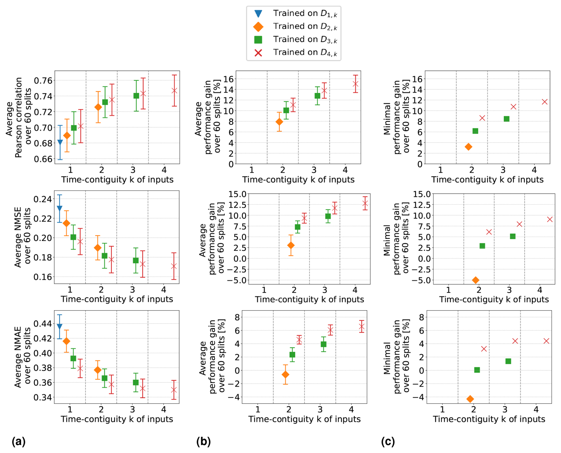
Figure 7 Linear regression models trained on D_M,k for M ≤ 4 with different time contiguities k. Performance on D_4,k has been evaluated through six-times 10-fold spatial cross-validation. Panel (a) shows the average performance over all 60 station splits for three performance measures. Panel (b) shows the average performance gain relative to the best case of k = 1; see Eq. (6) for the definition of performance gain. Error bars illustrate the standard deviation. Panel (c) shows the minimal performance gain. Across each row the same performance measure is considered. The exact values in panels (a) and (b) can be found in Table B2.

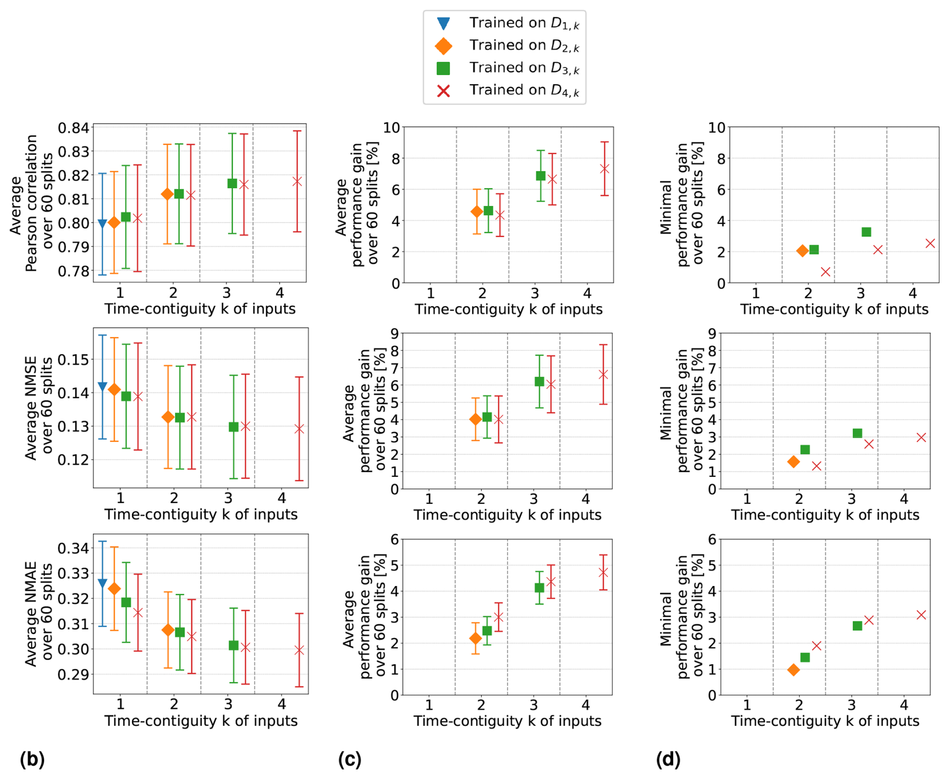
Figure 8 Same as Fig. 7 but for random forests trained on D_M,k for M ≤ 4 with different time contiguities k. Performance on D_4,k has been evaluated through six-times 10-fold spatial cross-validation. Panel (a) shows the average performance over all 60 station splits for three performance measures. Panel (b) shows the average performance gain relative to the best case of k = 1; see Eq. (6) for the definition of performance gain. Error bars illustrate the standard deviation. Panel (c) shows the minimal performance gain. Across each row the same performance measure is considered. The exact values in panels (a) and (b) can be found in Table B3.

For individual splits, we consider the performance gains that models with time contiguity k > 1 achieve compared to models with no time contiguity (k = 1). Since, in contrast to Experiment 1, we are now dealing with four different training cases for k = 1, we slightly adapt the definition of performance gains from Eq. (5): for a given split into training and test stations and fixed N, let E_M,k be the test performance (e.g., correlation) on D_N,k achieved by a model trained on D_M,k. We define the performance gain achieved by this model in Experiment 2 as

$$\begin{array}{}\text{(6)}& min\left\{{\displaystyle \frac{E_{P,\mathrm{1}}-E_{M,k}}{E_{P,\mathrm{1}}-E_{\mathrm{opt}}}}:P\in \mathit{\{}\mathrm{1},\mathrm{\dots },\mathrm{5}\mathit{\}}\right\}.\end{array}$$

In other words, for each split, the performance gain is always computed with respect to the best model trained without time contiguity (k = 1).

Average performance gains are depicted in Figs. 7b and 8b, which differ only slightly from those in Experiment 1, as models trained on D_4,1 are better, on average, than models trained on D_M,1. Linear regression models trained with k = 4 still achieve performance gains of 15.0 % in correlation, 12.8 % in NMSE, and 6.6 % in NMAE, whereas random forests achieve average gains of around 7.3 %, 6.6 %, and 4.7 %, respectively. Again, we observe that improvements over k = 1 are not only true on average, but also for each individual split: Figs. 7c and 8c show the minimal performance gains over all 60 splits. It shows that linear regression models for k = 4 always achieve an improvement of at least 11.7 % in correlation, 9.1 % in NMSE, and 4.4 % in NMAE. Random forests achieve gains of at least 2.5 %, 3.0 %, and 3.1 %, respectively. Hence, models with a larger time contiguity k > 1 provide reliable and statistically significant improvements (with respect to the performance measures) compared to models with no time contiguity (k = 1). Similar observations are made for the coefficient of determination and the index of agreement, two further performance measures. Definitions can be found in Appendix A and achieved performances in Tables B2 and B3 in Appendix B.

So far, we have discussed the test case N = 4 in detail. In the remainder of this section, we briefly summarize our similar observations for general $N\in \mathit{\{}\mathrm{2},\mathrm{3},\mathrm{4},\mathrm{5}\mathit{\}}$: for all N, we observed that the best test performances on D_N,k are achieved when training on D_N,N, i.e., with time contiguity k = N. If N = 5, we observe that there is barely any difference between training on D_5,5 and training on D_4,4, which implies that it is not required to use a larger time contiguity than k = 4. Also, for the general test case N, models trained with time contiguity k > 1 achieve reliable performance gains over models trained with k = 1. Results for the test case D_2,k are illustrated in Figs. C2 and C3 in Appendix C.

Altogether, our findings demonstrate that it is indeed reliably beneficial to use time-contiguous input features for predicting surface NO₂, in spite of a smaller available training dataset, which answers our main research question. As a rule of thumb, consider the case where surface NO₂ is to be predicted at a given location and time for which input features are also available at j≥1 previous hours. Then use j^′ = $min\mathit{\{}\mathrm{3},j\mathit{\}}$ hours, in addition to the features at the current time, as input for a random forest that has been trained with time contiguity k = $j^{\prime }+\mathrm{1}$ on a dataset D_k,k. If features are not available at previous hours, use the random forest that has been trained without time contiguity. We have demonstrated within this experiment that time-contiguous models provide valuable support whenever they are applicable. An interesting future task would be to inspect whether a similar rule can be observed for other machine learning approaches.

Within this section, we analyzed the difference between time-contiguous models in terms of prediction accuracy. However, we did not systematically assess other potential differences that may arise when switching between models trained with different time-contiguous features. For practical applications, when combining these models to create surface NO₂ concentration maps, it remains an interesting avenue for future work to investigate whether the ensemble of such models yields consistent combined spatial patterns in predicted surface NO₂.

5.3 Experiment 3: influence of tropospheric NO₂ VCDs, latitude, and surface height

In Experiment 3, we compare the outcomes of Experiment 2 in four different settings regarding the input of the models, as described in Sect. 3.2:

•  

  Setting 1. All features selected in Sect. 3.1 are included as input features, which was the setting in Experiments 1 and 2.

•  

  Setting 2. VCDs are excluded as an input feature.

•  

  Setting 3. Latitude and surface height are excluded.

•  

  Setting 4. VCDs, latitude, and surface height are excluded.

In this section, we focus exclusively on random forests and discuss the test results on D_4,k for the four different settings above.

Setting 1 is discussed in the previous section, where the results are illustrated in Fig. 8. Equally detailed illustrations for the remaining three settings are provided in Appendix D. A direct comparison between the four settings is made in Fig. 9: panel (a) shows the average Pearson correlation, NMSE, and NMAE achieved by random forests within these four settings, while panel (b) displays the corresponding average performance gains. For clarity, we only include the results for the models trained on D_4,k for different time contiguities $k\in \mathit{\{}\mathrm{1},\mathrm{\dots },\mathrm{4}\mathit{\}}$, excluding the models trained on larger datasets D_M,k (similar to Experiment 1).

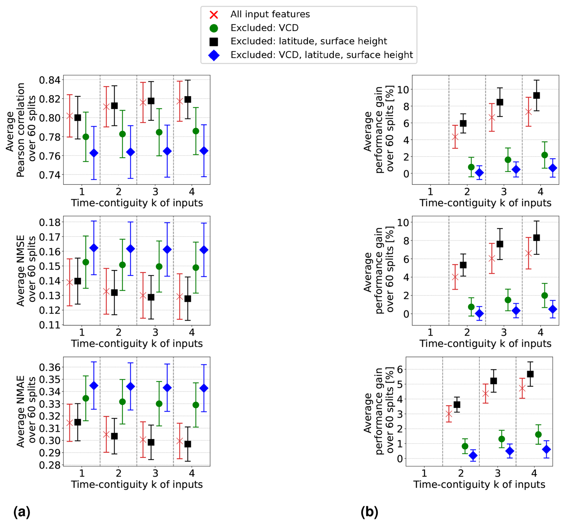
Figure 9 In the four settings of Experiment 3 (named in the legends of the plots), random forests are trained and tested on D_4,k for different time contiguities k. Performance is evaluated through six-times 10-fold spatial cross-validation. Panel (a) shows the average performance over all 60 station splits achieved within these four settings. Three performance measures are considered, one for each row. Error bars illustrate the standard deviation. Panel (b) shows the average performance gain relative to the best case of k = 1; see Eq. (6) for the definition of performance gain.

In Setting 3, where latitude and surface height are excluded, the models achieve similar results to those in the original Setting 1. Results are even slightly better without using these coordinates if k > 1. Moreover, the benefit of using time-contiguous input features is larger in Setting 3: average performance gains, calculated with Eq. (6), achieved when training on D_4,k are 9.3 % in Pearson correlation, 8.3 % in NMSE, and 5.7 % in NMAE. The minimum gains across all 60 station splits are 5.4 %, 3.7 %, and 3.8 % in correlation, NMSE, and NMAE, respectively (see Fig. D1). This implies that, similar to Setting 1, including time-contiguous features also provides a reliable improvement in Setting 3. This observation that coordinates are not required as inputs to make good predictions is promising, since it presumably increases the models' chances to also perform well outside of South Korea. Nevertheless, this hypothesis remains to be investigated within further research.

When excluding the tropospheric NO₂ VCDs (Setting 2), all performance measures decline, which is expected because the VCDs correlate the most among all input features with the surface NO₂ measurements. Despite this, the performances remain acceptable. For instance, with time contiguity k = 1, the average Pearson correlation in Setting 2 is 0.78, whereas it is about 0.8 in Settings 1 and 3, when VCDs are included. Interestingly, without VCDs in Setting 2, the average performance gains achieved with larger k are significantly lower: in Setting 2, the average performance gain is around 2 %, whereas in Settings 1 and 3, it is 3.5 and 4.5 times larger, respectively. Consequently, for time contiguity k = 4, the difference in performance is larger: models in Setting 2 achieve an average correlation of 0.786, while those in Settings 1 and 3 reach almost 0.82. When tropospheric NO₂ VCDs, latitude, and surface height are excluded in Setting 4, not only do performances weaken further, but the performance gains also drop below 1 %. In Setting 4, the average correlation is below 0.765 for all k. Similar trends are observed for NMSE and NMAE. This indicates that spatial coordinates play a more critical role when VCDs are excluded, which presumably leads to models that are less capable of generalizing to locations outside of South Korea. Inspecting the connection between including VCDs and the model's ability to generalize to locations outside of South Korea remains an interesting task for the future.

Furthermore, when tropospheric NO₂ VCDs are excluded, in both Setting 2 and Setting 4, the use of time-contiguous inputs no longer provides a reliable improvement. Across the 60 station splits, the performance gain is not always positive, which can be seen in Fig. 9b. Due to this observation that improvements by time-contiguous inputs are only reliable when including VCDs, the following question arises: how is performance affected if VCDs are treated as the only time-contiguous input feature? The experiments covering this case are illustrated in Fig. D4 in Appendix D. We observe that the average performances and average performance gains are higher if the other features are also considered time contiguous. Therefore, one future task could be to find the optimal choice of time contiguity k for each input feature individually.

At the end of this section, we show in Fig. 10 an example of how predictions of surface NO₂ appear on a map for the four investigated settings. We consider latitudes and longitudes within 32° N, 39° N and 124° E, 132° E, respectively. GEMS tropospheric NO₂ VCDs on 7 April 2021 from 01:45 to 02:15 UTC are shown in panel (a). We chose this time and day due to little cloud cover in the area and thus only a few missing satellite observations. Predictions of surface NO₂ from 01:00 to 02:00 UTC made by random forests are shown in panel (b) for Settings 1 and 3, whereas panel (c) covers the settings with tropospheric NO₂ VCDs excluded. All models have been trained with time contiguity k = 4 on D_4,4.

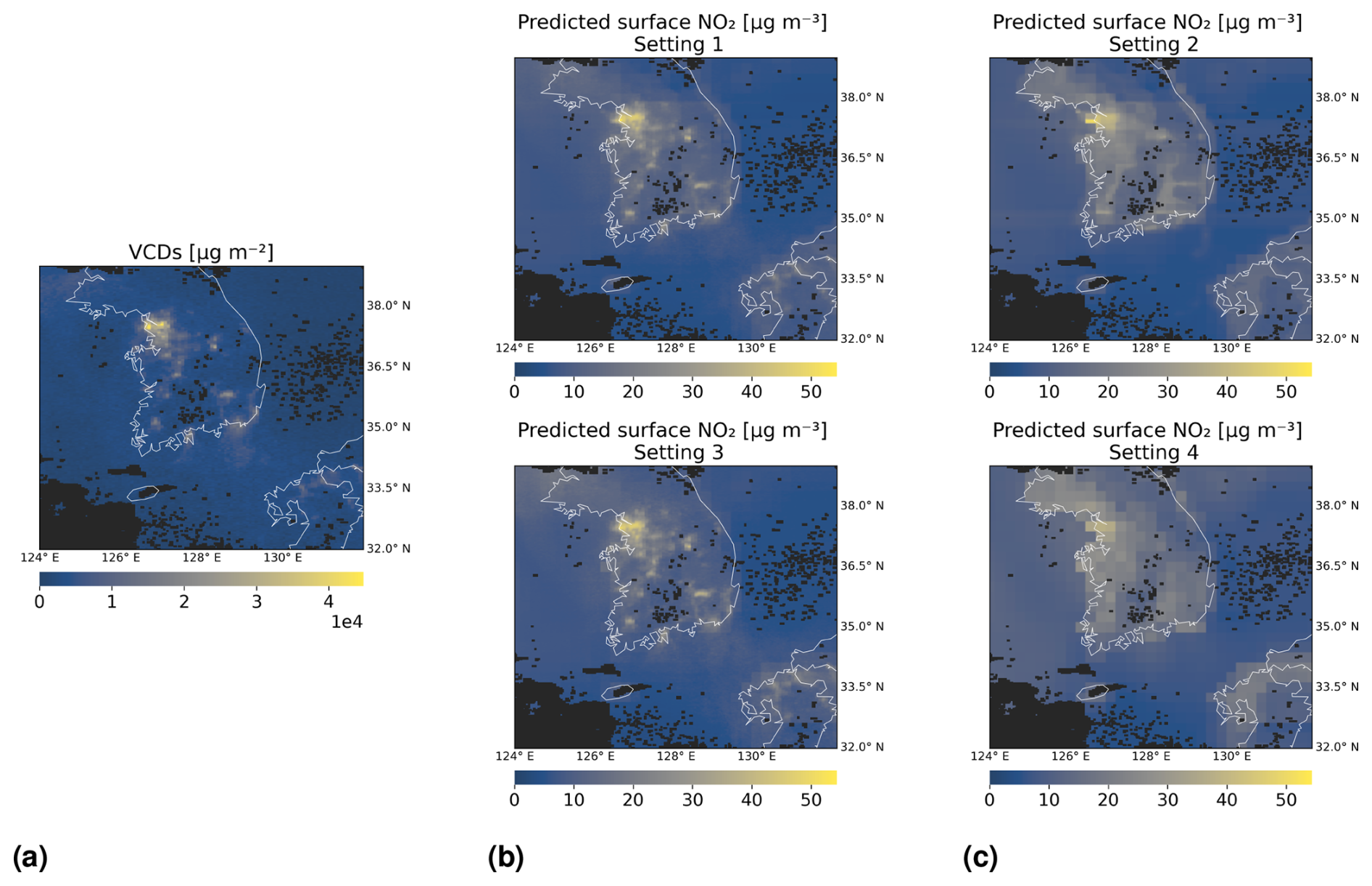
Figure 10 Predictions of surface NO₂ by random forests on 7 April 2021 from 01:00 to 02:00 UTC, for Settings 1–4 of Experiment 3. Panel (a) shows tropospheric NO₂ VCDs from 01:45 to 02:15 UTC. Panel (b) shows predicted surface NO₂ in Settings 1 and 3, when VCDs are included as input. Panel (c) shows predictions in Settings 2 and 4, when VCDs are excluded. In the second row of panels (b) and (c), latitude and surface height are excluded. The black mask indicates missing data, e.g., due to clouds. All models have been trained with time contiguity k = 4 on D_4,4 for the same choice of training stations.

We observe that there is a high similarity between predictions made in Settings 1 and 3, when tropospheric NO₂ VCDs are included as input features. This is in agreement with our findings from Fig. 9 that in both settings similar results are achieved regarding all considered performance measures. This observation is promising, as excluding latitude and surface height reduces the spatial bias of the model, which is to be tested in future studies. Therefore, presumably, the model's chance of making suitable predictions in different parts of the world increases. In Settings 1 and 3, the impact of the tropospheric NO₂ VCDs on the prediction of surface NO₂ is directly visible, since the hotspots of the VCDs and predictions of surface NO₂ are depicted at the same locations. On the other hand, when VCDs are excluded in Settings 2 and 4, these hotspots are less recognizable due to a smaller contrast to their neighborhood; see Fig. 10c. In Settings 2 and 4, the predicted surface NO₂ has a coarser resolution, which is to be expected considering that the resolution of meteorological inputs is 8 times coarser compared to the VCDs. In all four settings, the contrast between the hotspots and the background of predicted surface NO₂ is less pronounced compared to the contrast observed in the tropospheric NO₂ VCDs shown in panel (a). This effect is even more evident in another example from 27 February 2022, shown in Fig. 11. Notably, the predicted concentrations of surface NO₂ over water are only slightly smaller compared to those over land within all settings, even in regions far from the coast, such as the southeastern parts of the maps. However, emissions over water are not expected, aside from maritime traffic. Furthermore, at some distance from the coast, no contribution from land-based emissions is expected due to the short atmospheric lifetime of NO₂. Consequently, both the tropospheric NO₂ VCDs and the surface NO₂ concentrations should be low in these areas. Given the predicted surface concentrations of approximately 7 µg m⁻³, it appears that the models have likely overestimated surface NO₂ concentrations in these areas over water. This aligns with the observation from Fig. 6, which shows that the models tend to overestimate low surface NO₂ values. A possible explanation for this could be that the models were trained only on data from stations located on land or islands.

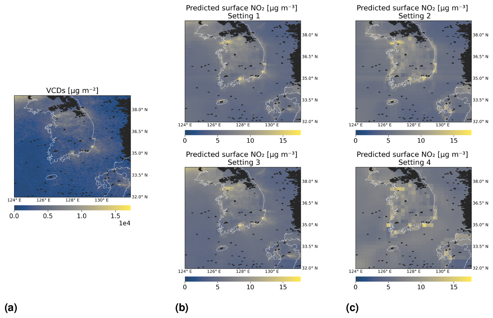
Figure 11 Same as Fig. 10 but on 27 February 2022. Panel (a) shows the VCDs from 06:45 to 07:15 UTC. Panels (b) and (c) show predicted surface NO₂ from 06:00 to 07:00 UTC, for the four settings of Experiment 3.

5.4 Seasonal and diurnal error distribution

In the previous sections, the performance of machine learning models is evaluated using whole-year data, spanning January 2021 to November 2022. In this section, we inspect how prediction quality varies across different seasons and throughout the day. Some variation is expected, as the accuracy of GEMS observations also fluctuates. For example, accuracy tends to be lower in the morning due to the shallow boundary layer (Yang et al., 2023a). For the remainder of this section, we focus on the best-performing models identified in our earlier analysis. Specifically, we reconsider the random forest models from Setting 3 in Sect. 5.3, which do not incorporate spatial coordinates as input features. These models were trained on all respective training datasets D_N,k, but for this section, their performance is spatially cross-validated on the test datasets for different seasons and times of the day individually. For simplicity, we restrict our attention to models that were trained on the dataset D_4,k. Furthermore, we inspect whether benefits from time-contiguous inputs depend on the season or time of the day.

First, we compare the test performance across different seasons. Each season in South Korea is typically defined as a 3-month period: spring (March–May), summer (June–August), autumn (September–November), and winter (December–February). Table 3 shows the percentage of data points in D_4,k belonging to each season. Notably, summer has the fewest valid data points due to the applied filter for the qa value during data preprocessing. In addition, the Pearson correlation between surface NO₂, measured at the in situ stations, and VCDs is the lowest in summer (see Table 3). These factors likely contribute to the significantly lower performance of the random forest models in summer compared to other seasons (see Fig. 12). In contrast, the model performance is the highest in winter across all performance measures, i.e., for Pearson correlation, NMSE, and NMAE. Moreover, we observe that within each season, incorporating time-contiguous inputs improves prediction quality. The performance gains, calculated using Eq. (5), are also shown in Fig. 12. Notably, the largest gains from time-contiguous inputs occur in winter, exceeding 12 % in Pearson correlation for time contiguity k = 4. The smallest gains are observed in summer, with an improvement of only 5 % in Pearson correlation.

Table 3 Statistics for seasonal segments of the dataset D_4,k.

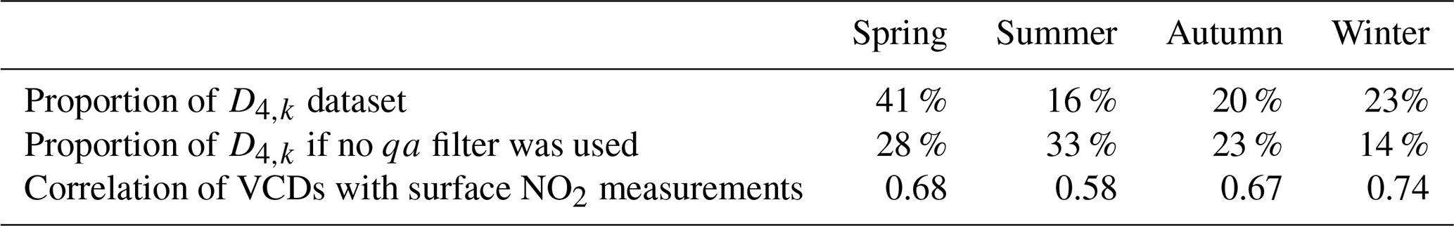
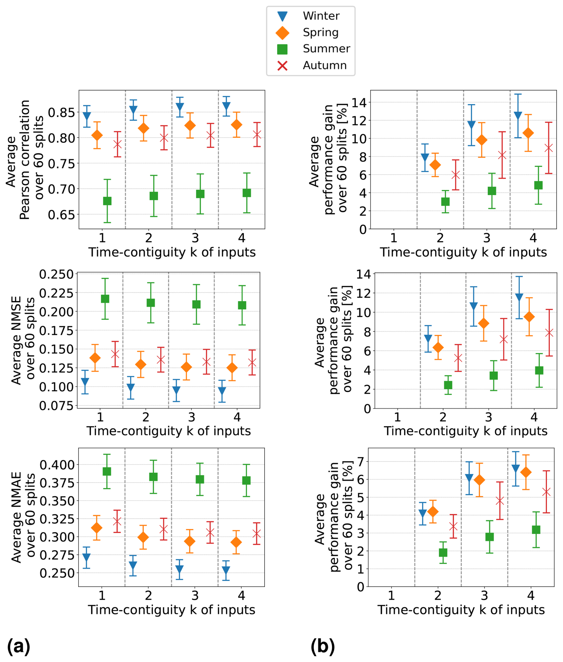
Figure 12 Random forests trained on D_4,k for different time contiguities k, without spatial coordinates as input features. Test performance is evaluated in different seasons (winter, spring, summer, and autumn) through six-times 10-fold spatial cross-validation. Panel (a) shows the average performance over all 60 station splits achieved in different seasons and for different k. Three performance measures are considered, one for each row. Error bars illustrate the standard deviation. Panel (b) shows the average performance gain relative to the case of k = 1; see Eq. (5) for the definition of performance gain.

Finally, the performance across different times of the day is illustrated in Fig. 13. Since we focus on training and testing on D_4,k, the earliest time window with available data is 10:00–11:00 Korean standard time (KST). The best performance is achieved around midday, while the performance declines in the morning and afternoon. The worst results occur between 16:00 and 17:00 KST, possibly due to the fact that surface NO₂ has the weakest correlation with VCDs at that time (see Table 4). Moreover, it should be noted that for datasets D_N,k with N ≤ 3, in which data points at times earlier than 10:00 KST occur, the performance is expected to further decrease compared to the later morning hours.

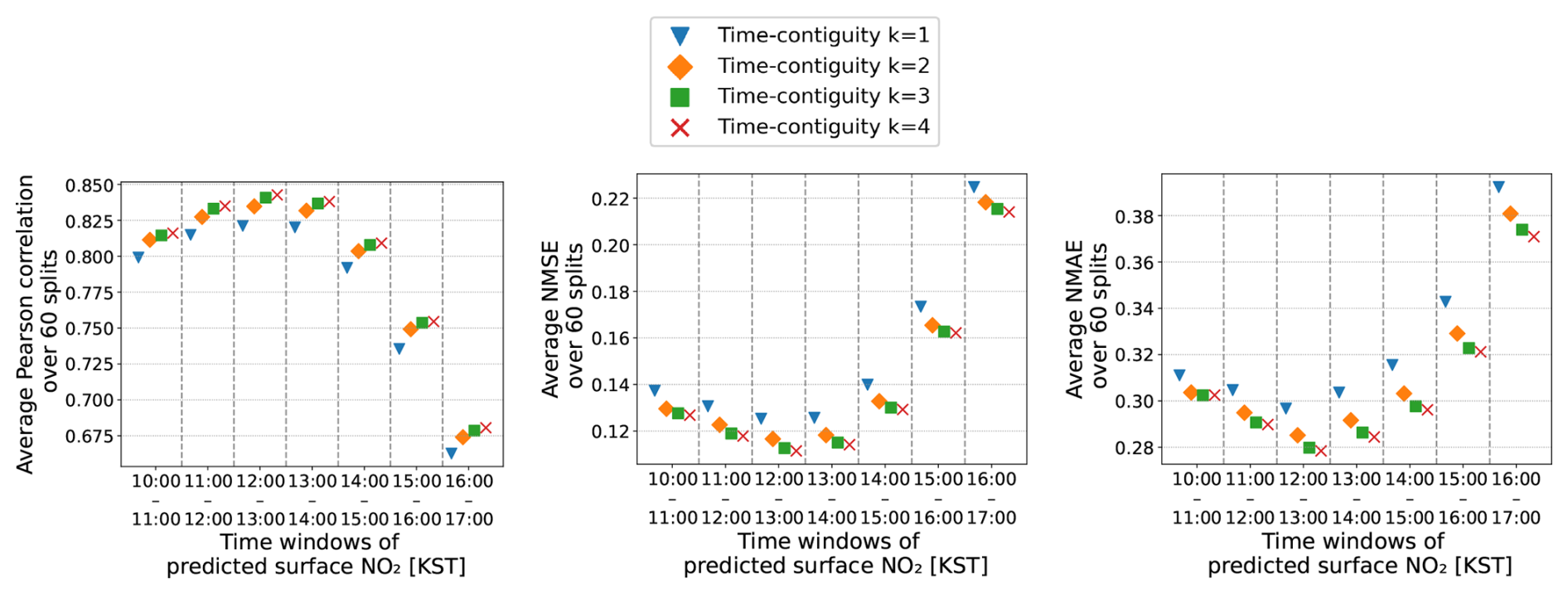
Figure 13 Same random forests as in Fig. 12 but the test performance is cross-validated at different times of the day. The time windows are chosen in line with the in situ dataset. Korean standard time (KST) is used.

Table 4 Statistics for different hourly segments of the dataset D_4,k.

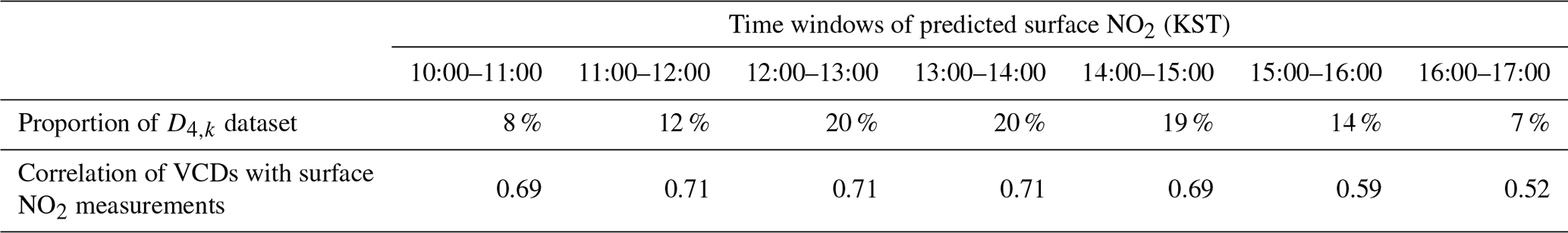
Furthermore, at all times, time-contiguous models consistently outperform models with no time contiguity k = 1, demonstrating a clear benefit from using time-contiguous input features.

6 Conclusions and outlook

For the first time, hourly tropospheric NO₂ VCDs are available thanks to the geostationary satellite of the GEMS instrument platform. To predict surface NO₂ levels at a given time and location, we proposed to also include VCDs and meteorological features from previous hours as inputs to the machine learning models.

Our main research question was whether the considered machine learning models, random forests and linear regression, benefit from hourly time-contiguous input features for the prediction of surface NO₂. We observed that using time-contiguous input features led to reliable enhancements with respect to all considered performance measures, as long as tropospheric NO₂ VCDs were included. For random forests, average performance gains were between 4.5 % and 7.5 % depending on the performance measure. For linear regression models, average performance gains were larger, namely between 7 % and 15 %. This is to be expected since the non-linear structure of random forests allows for the extraction of more information from non-time-contiguous inputs, generally also leading to better predictions compared to linear regression models. These improvements were reliable in the sense that positive performance gains were achieved not only on average, but also across all 60 splits into training and test in situ stations during spatial cross-validation. Moreover, we were able to demonstrate that performance gains were observed despite having much fewer data points available for training models with a larger time contiguity of their inputs. As a rule of thumb, for the case where tropospheric NO₂ VCDs are used as an input feature, we suggest the following: whenever surface NO₂ is to be predicted at a given location and time for which input features are available at j previous hours, feed those features, together with those at the current time, into a random forest that has been trained with time contiguity k = $min\mathit{\{}j+\mathrm{1},\mathrm{4}\mathit{\}}$ on a given training dataset D_k,k, specified in Sect. 2.3. If features are not available at previous hours, one cannot use a time-contiguous model to make a prediction for these data points, so one has to use the random forest that has been trained without time contiguity. Therefore, time-contiguous models should be understood as a supportive tool that should be applied whenever possible. Whether the rule of thumb above still applies to other machine learning models, such as neural networks or extreme gradient boosting, would be an interesting aspect for future studies.

Furthermore, when tropospheric NO₂ VCDs were included as input in the models, we observed that latitude and surface height were not required for achieving similar performances and benefits from time-contiguous inputs. Presumably, this increases the chance that the models will also provide good predictions beyond South Korea, which will be an interesting investigation for future work. If validated, this would enhance the model's flexibility and broader applicability without the requirement of more training data, and hence longer training time, from different regions. Another task would be to determine the optimal time contiguity for every input feature individually, which would reduce redundancy among input features and hence lead to better performances.

When tropospheric NO₂ VCDs were excluded as input features, performance worsened but remained within an acceptable range. Additionally, we observed that the benefit of time-contiguous features was significantly reduced, and the performance gain was no longer reliable. Specifically, across all 60 splits during spatial cross-validation, benefits were not consistently observed. When both VCDs and spatial coordinates were excluded, performance decreased further. This indicates that spatial coordinates play a more critical role when VCDs are not included, which presumably leads to models that are less capable of generalizing to locations outside of South Korea. Again, this motivates further research on the connection between including VCDs and the models' ability to generalize to locations outside of South Korea.

Last but not least, we would like to address the time coverage of the data, which spans January 2021 to November 2022. Although data from December 2022 are missing, Sect. 5.4 shows that random forests performed best on winter data. It would be interesting to investigate whether models perform even better for a specific season when trained exclusively on data from that season. We leave this for future investigation. Furthermore, the Covid-19 pandemic occurred during the considered data time window, resulting in emissions that differ from those observed in non-pandemic conditions. This bias should be considered when applying models trained on Covid-19 data to pandemic-free settings.

Appendix A: Further performance measures

In the following we describe further scale-insensitive performance measures to fill the gap between surface NO₂ measurements $x^{†}\in {\mathbb{R}}^n$ and predictions x made by a machine learning model.

Coefficient of determination (R²).

$$R^{\mathrm{2}}\left(x^{†},x\right)=\mathrm{1}-{\displaystyle \frac{\sum _{i=\mathrm{1}}^n\mathrm{|}{x}_i^{†}-x_i\mathrm{|}}{\sum _{i=\mathrm{1}}^n\mathrm{|}{x}_i^{†}-{\stackrel{\mathrm{‾}}{x}}^{†}\mathrm{|}}},\text{where}{\stackrel{\mathrm{‾}}{x}}^{†}={\displaystyle \frac{\mathrm{1}}{n}}\sum _{i=\mathrm{1}}^n{x}_i^{†}$$

Note that R² is similar to NMAE, but normalization is done by the mean absolute deviation of x^† instead of its mean. Further, within the literature, the expression R² sometimes stands for the square of the correlation coefficient. However, in general, these definitions are not equivalent.

Index of agreement (IOA).

$$\text{IOA}\left(x^{†},x\right)=\mathrm{1}-{\displaystyle \frac{\sum _{i=\mathrm{1}}^n\mathrm{|}{x}_i^{†}-x_i{\mathrm{|}}^{\mathrm{2}}}{\sum _{i=\mathrm{1}}^n{\left(\mathrm{|}{\stackrel{\mathrm{‾}}{x}}^{†}-x_i\mathrm{|}+\mathrm{|}{\stackrel{\mathrm{‾}}{x}}^{†}-x_i^{†}\mathrm{|}\right)}^{\mathrm{2}}}}$$

Here ${\stackrel{\mathrm{‾}}{x}}^{†}$ denotes the mean of all $x_i^{†}$.

Appendix B: Tables

Table B1 Features considered during feature selection in Sect. 3.1. For 200 splits into training and test stations, the Pearson correlation with surface NO₂ was computed on the training set for each available feature. Average correlations are shown in the last column.

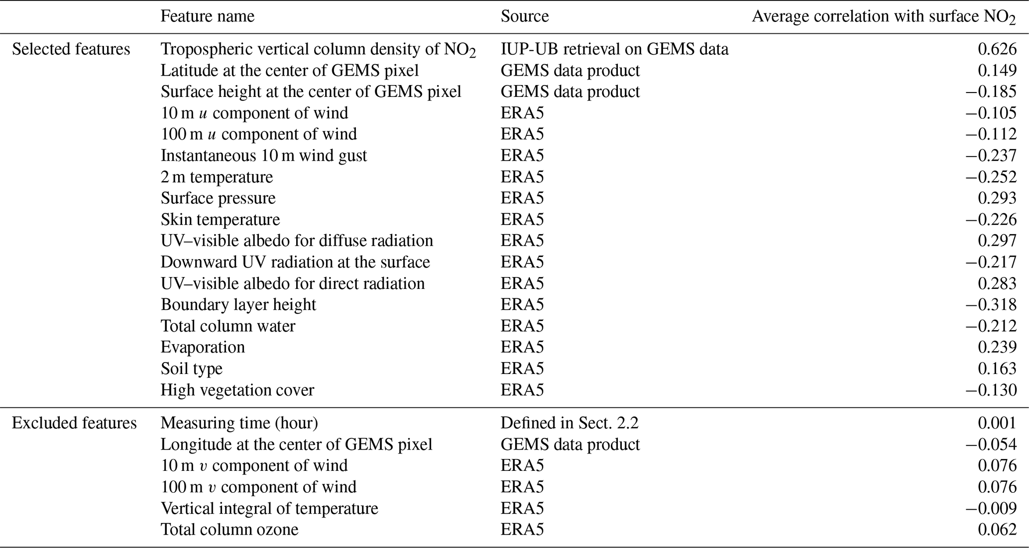
Table B2 Linear regression models have been trained on D_N,k for N ≤ 4 with different time contiguities k and input features selected in Sect. 3.1. Performance on D_4,k has been evaluated through six-times 10-fold spatial cross-validation. Five different performance measures are considered, defined in Sect. 3.3 and Appendix A. The best results are marked in bold.

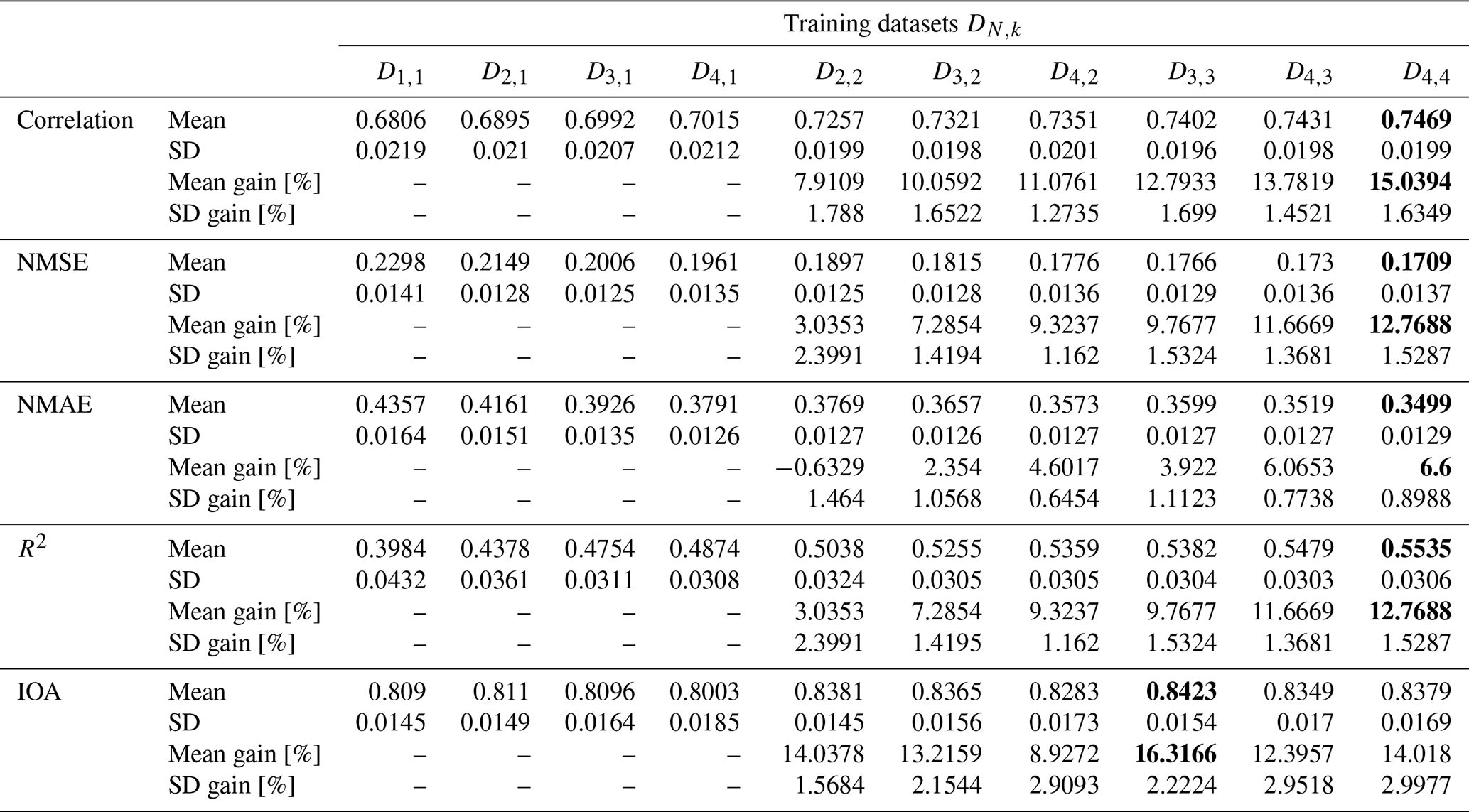
Table B3 Random forests have been trained on D_N,k for N ≤ 4 with different time contiguities k and input features selected in Sect. 3.1. Performance on D_4,k has been evaluated through six-times 10-fold spatial cross-validation. Five different performance measures are considered, defined in Sect. 3.3 and Appendix A. The best results are marked in bold.

Appendix C: Additional figures for Experiment 2

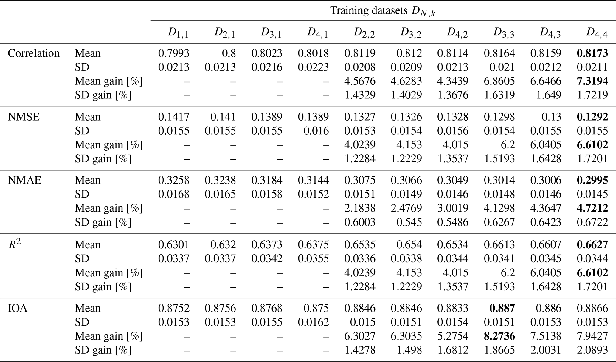
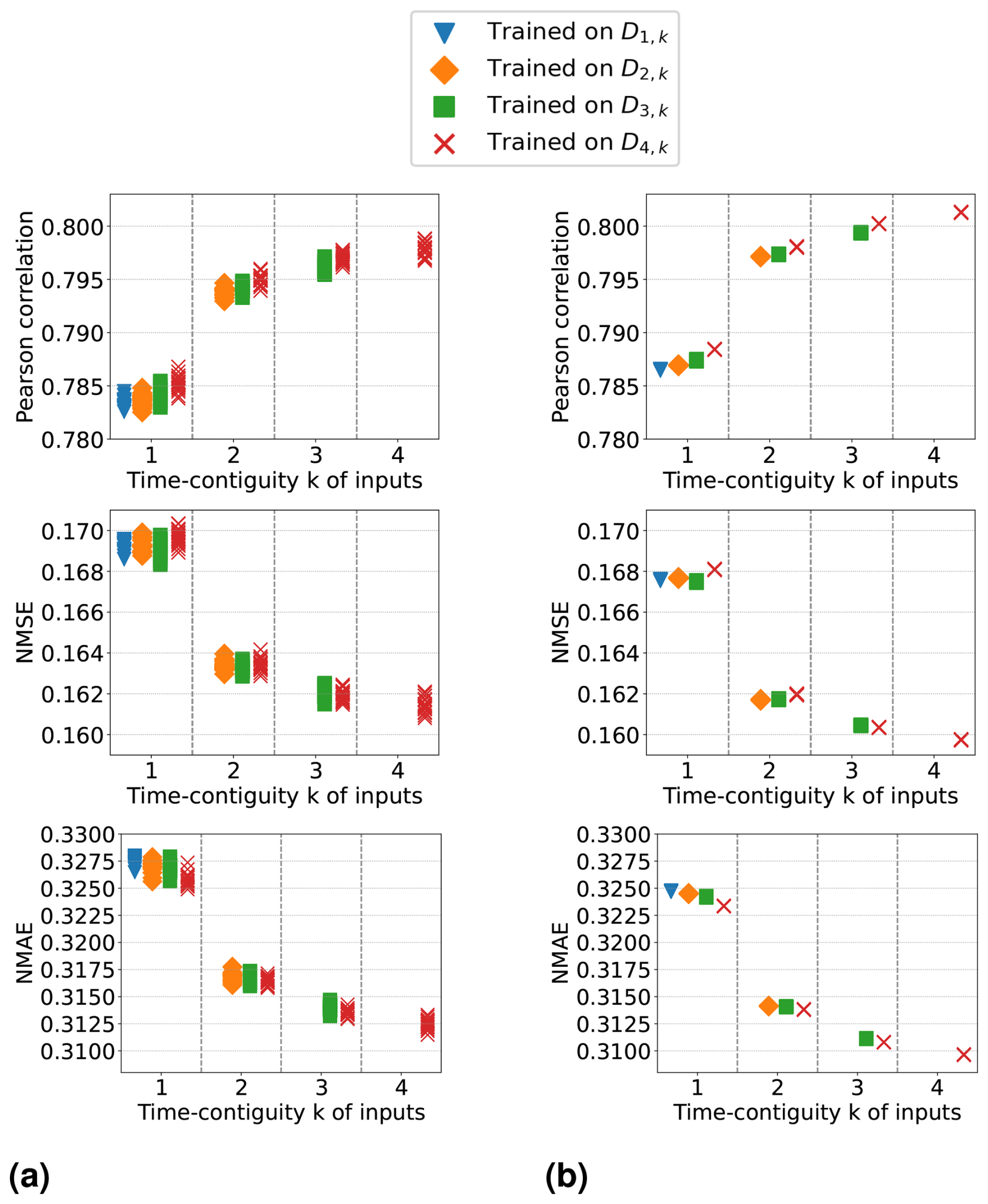
Figure C1 Random forests with 30 and 8000 trees (n_estimators) are considered in panels (a) and (b), respectively. Training and testing have been performed 20 times for the same split into training and test stations. Testing was on the corresponding dataset D_4,k, and training was on different D_M,k for M ≤ 4. Results for 20 individual repetitions are shown with respect to three performance measures.

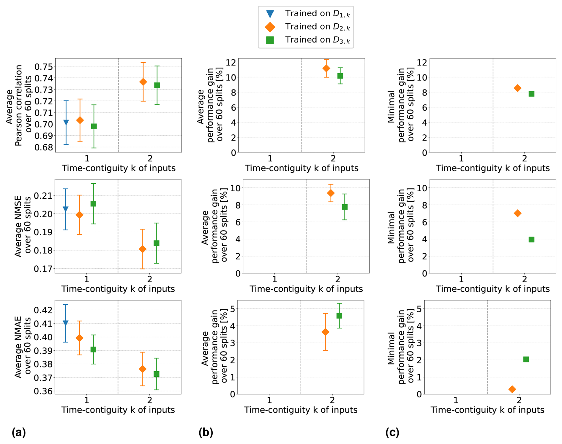
Figure C2 Linear regression models have been trained on D_M,k for M ≤ 3 with different time contiguities k and input features selected in Sect. 3.1. Performance on D_2,k has been evaluated through six-times 10-fold spatial cross-validation. Panel (a) shows the average performance over all 60 station splits for three performance measures. Panel (b) shows the average performance gain (Eq. 6) relative to the best case of k = 1. Error bars illustrate the standard deviation. Panel (c) shows the minimal performance gain. Across each row the same performance measure is considered.

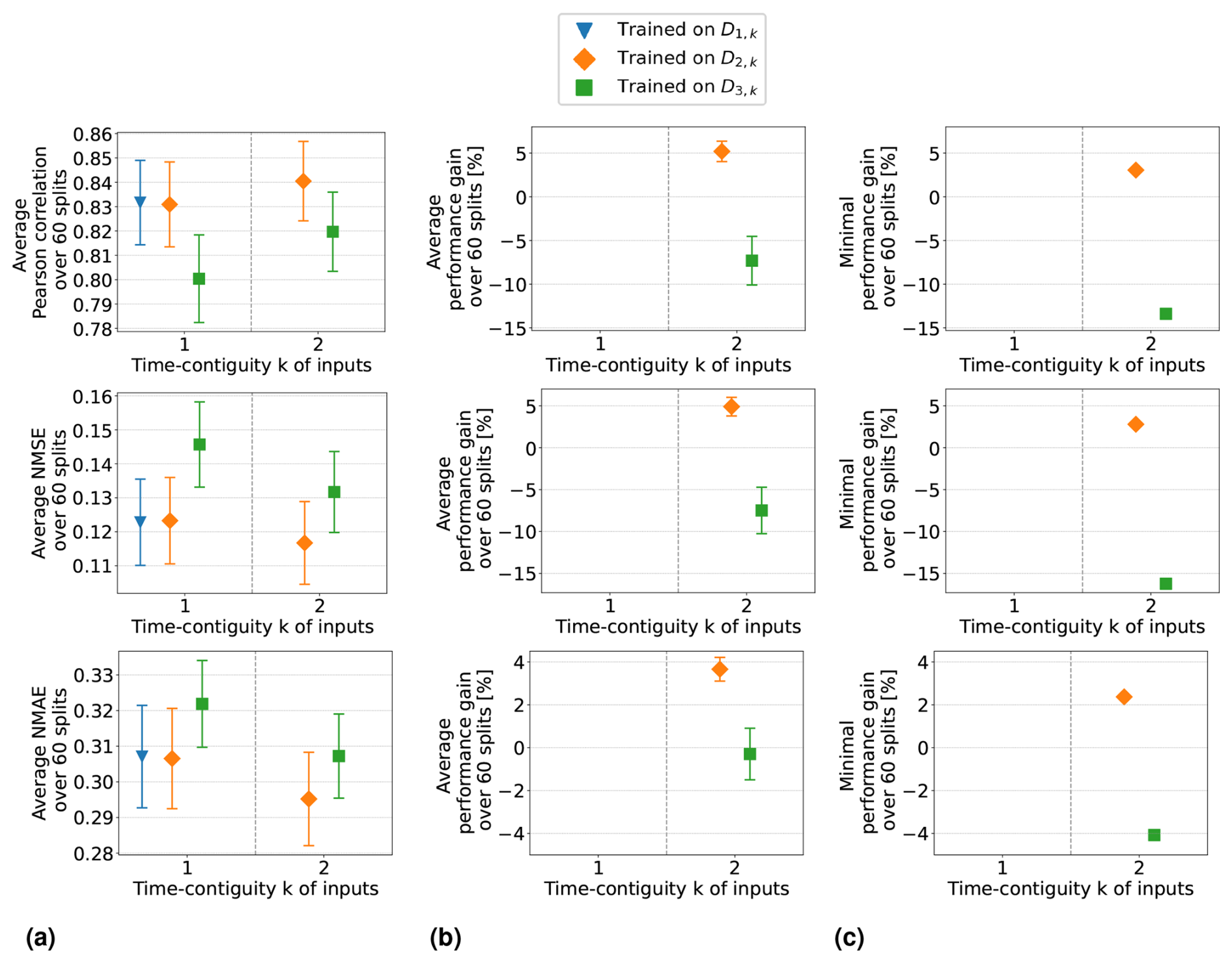
Figure C3 Same as Fig. C2 but for random forests trained on D_M,k for M ≤ 3 with different time contiguities k and input features selected in Sect. 3.1. Performance on D_2,k has been evaluated through six-times 10-fold spatial cross-validation. Panel (a) shows the average performance over all 60 station splits for three performance measures. Panel (b) shows the average performance gain (Eq. 6) relative to the best case of k = 1. Error bars illustrate the standard deviation. Panel (c) shows the minimal performance gain. Across each row the same performance measure is considered.

Appendix D: Additional figures for Experiment 3

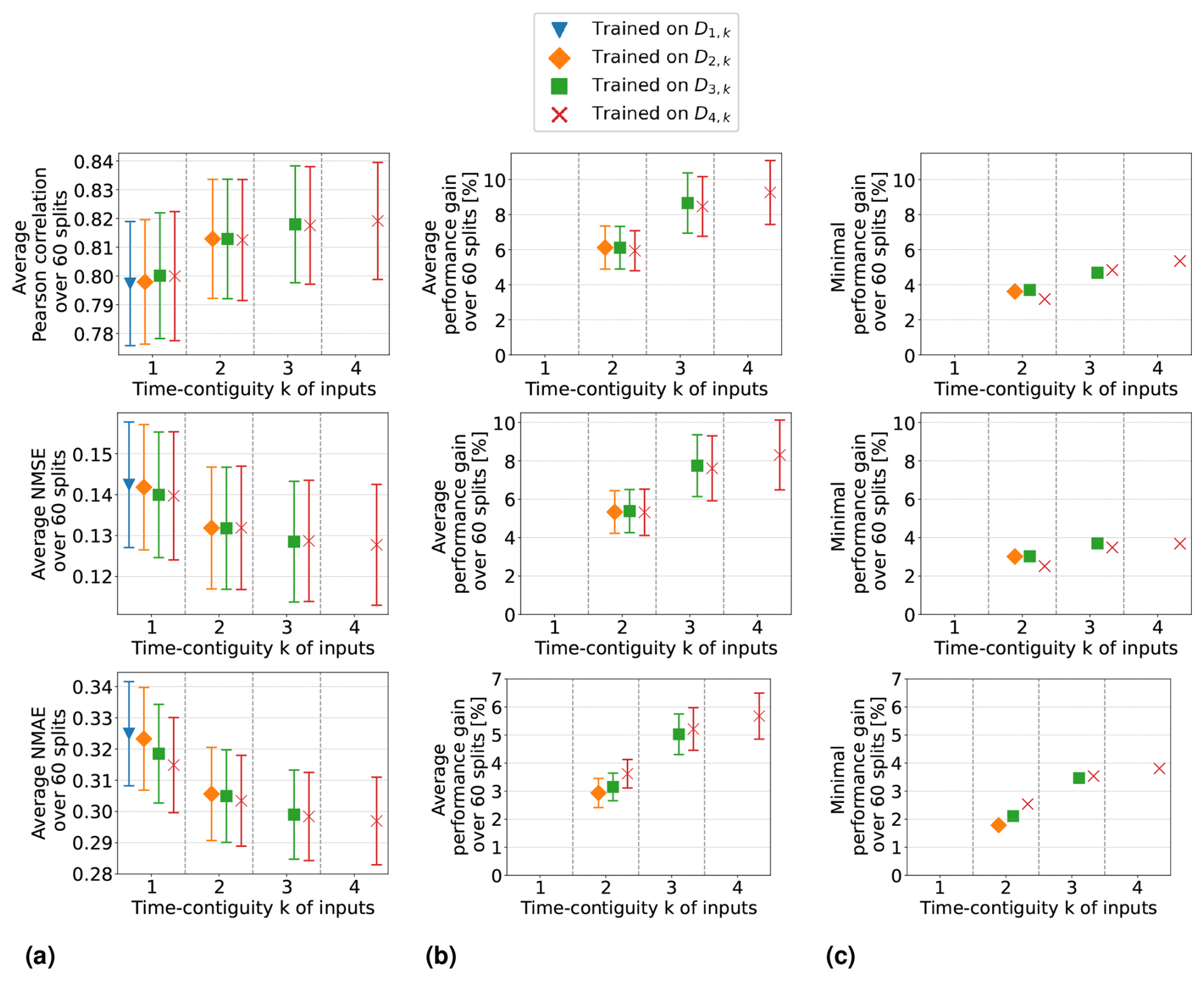
Figure D1 Excluded latitude and surface height from input features (Setting 3 of Experiment 3): random forests have been trained on D_M,k for M ≤ 4 with different time contiguities k. Performance on D_4,k has been evaluated through six-times 10-fold spatial cross-validation. Panel (a) shows the average performance over all 60 station splits for three performance measures. Panel (b) shows the average performance gain relative to the best case of k = 1; see Eq. (6) for the definition of performance gain. Error bars illustrate the standard deviation. Panel (c) shows the minimal performance gain. Across each row the same performance measure is considered.

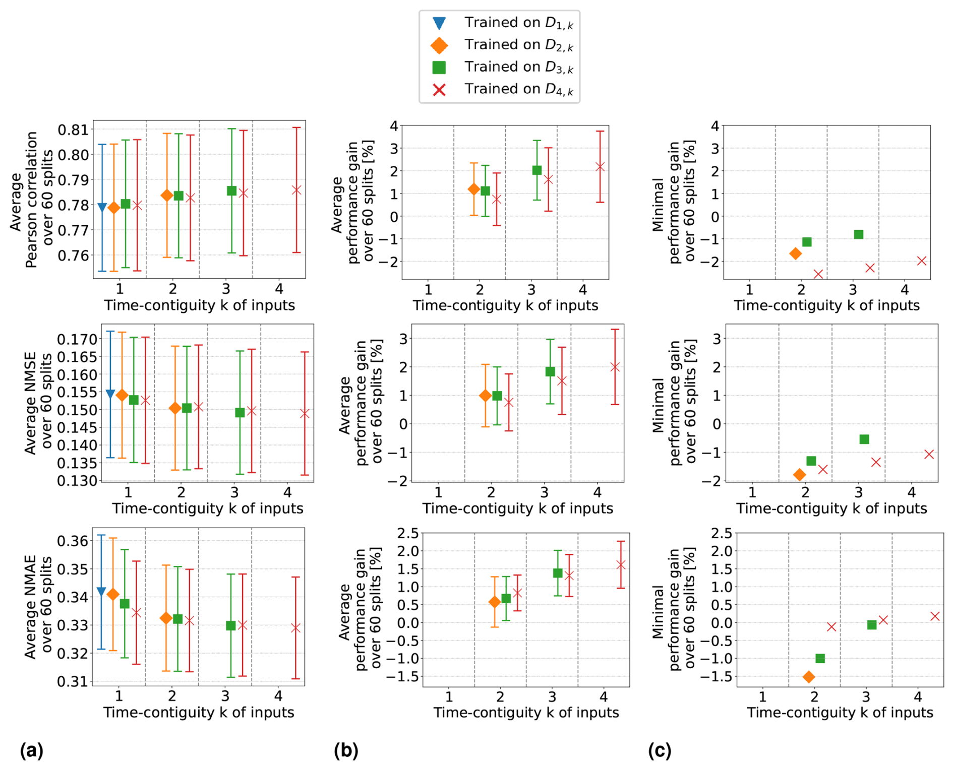
Figure D2 Same as Fig. D1 but excluding tropospheric NO₂ VCDs from input features (Setting 2 of Experiment 3).

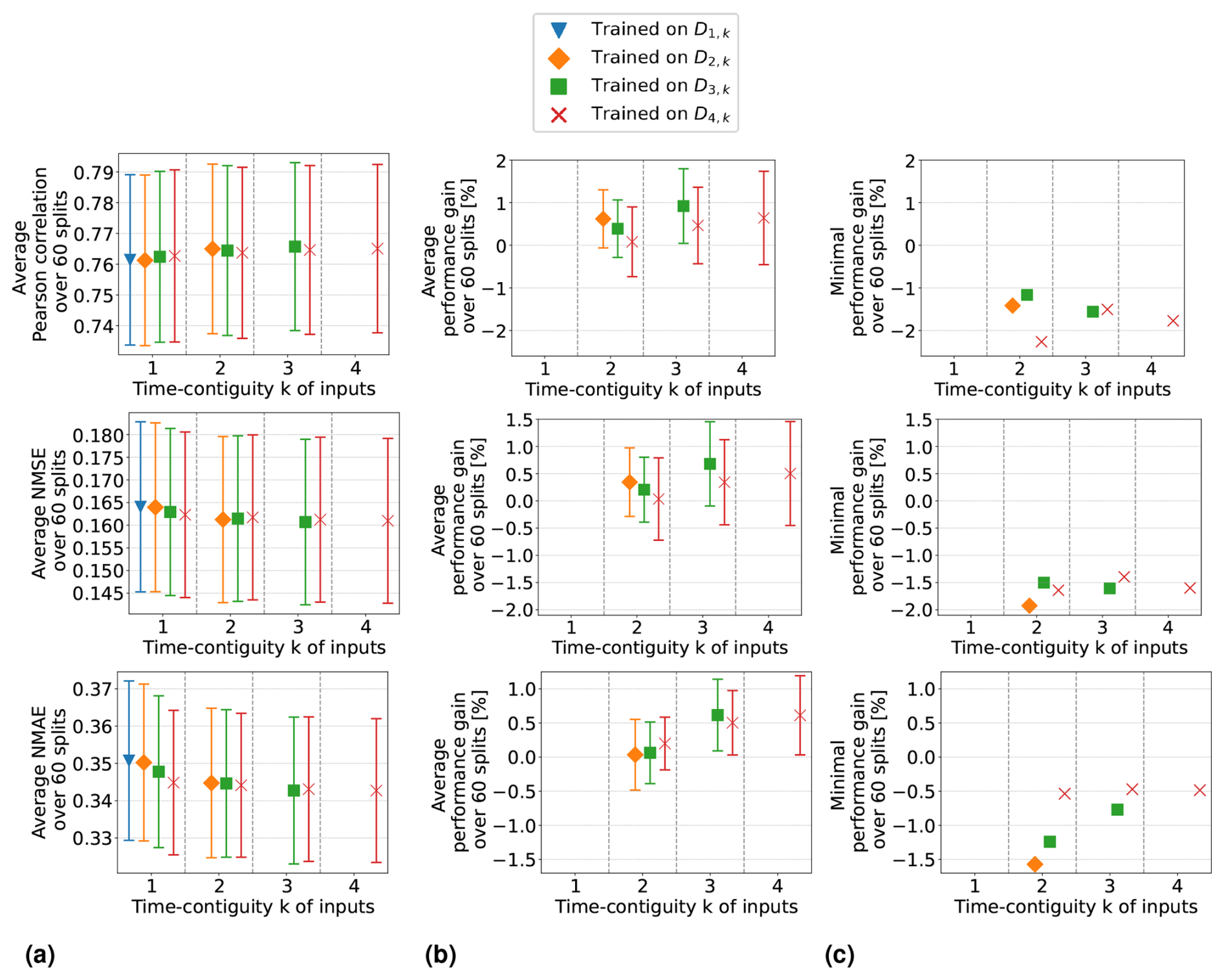
Figure D3 Same as Fig. D1 but excluding tropospheric NO₂ VCDs, latitude, and surface height from input features (Setting 4 of Experiment 3).

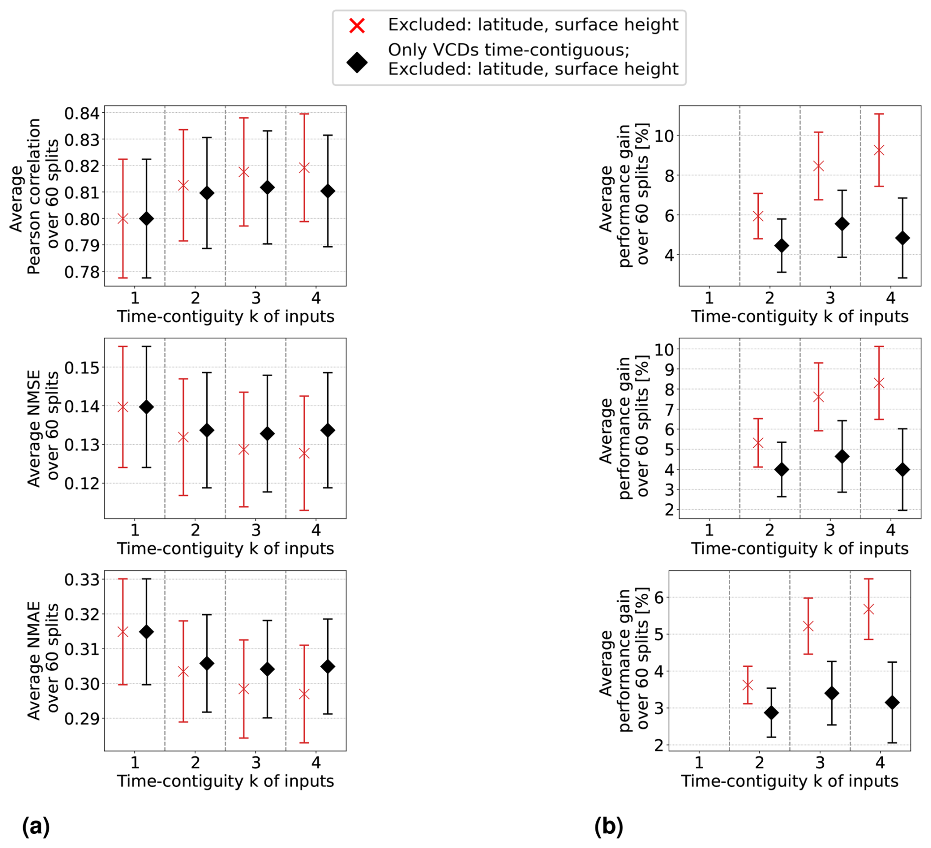
Figure D4 Random forests: the selection of input features is the same as in Setting 3 of Experiment 3; i.e., latitude and surface height are excluded. Comparison of two cases. First, only the time contiguity of tropospheric NO₂ VCDs is exploited. Second, the time contiguity of all (time-dependent) input features is exploited, which is exactly the same as Setting 3 of Experiment 3. Models have been trained and tested on D_4,k for different time contiguities k. Panel (a) shows the average performance from six-times 10-fold spatial cross-validation and panel (b) shows the average performance gain (Eq. 6).