Improving the accuracy in particle concentration measurements of a balloon-borne optical particle counter, UCASS

For balloon-borne detection of aerosols and cloud droplets (diameter 0.4 < D_p < 40 µm), a passive-flow Universal Cloud and Aerosol Sounding System (UCASS) was used, whose sample flow rate is conventionally derived from balloon ascent rates using GPS or pressure measurements. Improvements are achieved by implementing thermal flow sensors (TFSs) 94 mm downstream of the UCASS detection region for continuously measuring true UCASS sample flow velocities. UCASS-mounted TFSs were calibrated during wind tunnel experiments at up to 10 m s⁻¹, and under various angles of attack (AOAs), as these vary during actual balloon ascents. It was found that the TFS calibration is determined with sufficient precision using three calibration points at tunnel flows of ∼ 2, 5, and 8 m s⁻¹, simplifying efficient TFS upgrades of numerous UCASSs. In iso-axial alignment, UCASS flows are accelerated (by ∼ 11.3 %) compared to tunnel flows (at 2–8 m s⁻¹). In-flight comparisons up to 7.5 km in height revealed that UCASS sample flows rarely match the balloon's ascent rate. Laboratory experiments show that equality (v_GPS=v_TFS) is achieved only at AOA ≠ 0°, potentially affecting the UCASS internal flow pattern and particle transmission efficiency in flight. To minimise errors in calculated UCASS-based particle number concentrations, real-time measurements of the true UCASS flow velocity are recommended.

1 Introduction

Weather balloon soundings are an established method to carry out in situ measurements up to high altitudes in the atmosphere (e.g. Golden et al., 1986; Vömel and Fujiwara, 2021, or Vömel and Ingleby, 2023). Balloons filled with helium or hydrogen can reach heights of up to 40 km. Due to a moderately variable ascent rate of ∼ 5–6 m s⁻¹ on average, the troposphere and stratosphere are probed with a higher vertical resolution compared to aircraft measurement due to the higher climb and descent rates of the latter (at least 6 m s⁻¹ and usually more; cf. EUFAR, 2000). In conventional operation, a radiosonde is used as the payload, deployed on a thin cord of about 50–60 m length below the ascending weather balloon. Radiosondes are used to directly measure atmospheric pressure, humidity, temperature, and wind parameters during the ascent, while the data are sent in real time via radio to the receiving station (see, for example, Dirksen et al., 2020).

Balloon-based vertical soundings with radiosondes allow for characterising the current state of the atmosphere, from which atmospheric properties such as stability or stratification can be derived. The payload of the weather balloon can be extended beyond the sole use of radiosondes, for example by including an ozone probe (cf. Smit et al., 2024, and references therein) and/or optical particle counters (Matsumura et al., 2001; Kasai et al., 2003; Smith et al., 2019; Kezoudi et al., 2021; Snels et al., 2021). Both ozone, as an atmospheric trace gas, and aerosols and clouds have a major influence on the Earth system. Aerosols and clouds influence the Earth's energy balance (by absorbing and scattering short-wave radiation), the global water cycle (through the formation of precipitation), and atmospheric dynamics (through the conversion of latent heat in the phase transitions of water). Considering that aerosols and cloud droplets modify radiative fluxes (see, for example, Stier et al., 2024, or IPCC, 2023), a better understanding of their size, number, and vertical distribution is required and the vertical distribution of aerosols and cloud droplets needs to be frequently investigated. The University of Hertfordshire (UK) has developed an optical particle spectrometer for balloon soundings: the “Universal Cloud and Aerosol Sounding System” (UCASS; see Smith et al., 2019; Kezoudi et al., 2021; Girdwood et al., 2022; Girdwood, 2023; Schön et al., 2024) is used to detect aerosol particles and cloud droplets with diameters of 0.4 to 40 µm. The probe's measuring principle is described in detail in Sect. 2.

In general, the following thought model underlies the balloon sounding: the horizontal wind that causes the balloon to drift or influences its geographical position has almost no or a negligible influence on the inertial system of the balloon itself, unless gusty winds or strong wind shear prevails. Hence, regarding the horizontal wind component, there is almost no relative horizontal wind aboard the balloon or its payload. The predominant flow relative to the balloon and its payload that mainly drives the airflow through a UCASS is the vertical wind component, which in our case is determined by the balloon's lift, i.e. its ascent rate.

To calculate a particle number concentration from the particle number detected (per unit time) by a balloon-borne UCASS, the sample volume flow rate through the UCASS detection region must be known. Conventionally, the sample volume flow has been determined using balloon ascent rates (Kezoudi et al., 2021) derived from GPS or pressure measurements. This approach has two major disadvantages: (a) a zero horizontal wind velocity is inherently assumed and (b) changes in airflow caused by the instrument housing or small fluctuations remain unconsidered. One goal of this work therefore is to modify a UCASS such that a thermal flow sensor (TFS) is used to continuously determine the flow rates through a balloon-borne UCASS. This enables the accurate and precise determination of particle concentrations (and inferred microphysical quantities) at a higher confidence level. Beyond that, this study is a prerequisite for investigations based on UCASS measurements during our balloon missions in Central Europe during the summers of the years 2023 and 2024. Ultimately, the proposed improvements may provide support for UCASS applications by other users.

The present publication is structured as follows. First, the instrument is described. This is followed by reports on the testing and characterisation of the method of mechanically coupling the TFS to the UCASS (Sect. 2.5.1). Subsequently, the experiments aiming at the optimum position of the TFSs within the flow through a UCASS are described (Sect. 2.5.2). The TFSs are then calibrated against a reference flow sensor (Prandtl Pitot tube, PPt) within the flow through a UCASS (Sect. 2.5.3). Based on a numerical simulation, it has already been assumed that the flow velocity within the iso-axially aligned UCASS would increase by 12 % as compared to the ambient airflow speed of 5 m s⁻¹ (Smith et al., 2019). Therefore, in this work the PPt-measured ambient flow velocities and TFS-detected flow velocity inside the UCASS are compared (Sect. 3.2). The impact of a non-iso-axial alignment (i.e. when the angle of attack, AOA, towards the UCASS varies due to the balloon payload's pendulum motion) on the flow velocities through the UCASS and on the TFS calibration curves is investigated (Sect. 3.3 and 3.4). Finally, balloon soundings with the UCASS–TFS combination are used to prove the TFS performance under atmospheric conditions (Sect. 4). The findings are summarised in the conclusion section.

2 Instruments and methods

2.1 Universal Cloud and Aerosol Sounding System (UCASS)

The UCASS is an optical particle spectrometer (nominal detection range 0.4 < D_p < 40 µm; Smith et al., 2019; Girdwood, 2023). Due to its small size, low weight, and comparatively low cost (approx. EUR 2700 per unit), the UCASS is well suited for balloon soundings. The UCASS is of a tubular shape with 183 mm in length and with an outer diameter of 64 mm at a weight of about 280 g. A hollow flow tube with a quasi-elliptical cross-section of 40 mm × 30 mm diameter extends along the longitudinal axis of the UCASS, through which the sample air flows and in which the particles are detected. Particle detection with UCASS is carried out by optical detection of the scattered light caused by particles upon crossing a diode-emitted laser beam. The optical system of the UCASS defines a particle detection region of 0.5 mm² in size (Girdwood, 2023). In Fig. 1, the principal setup of the UCASS instrument is illustrated; for more details see Smith et al. (2019), Girdwood et al. (2022), or Girdwood (2023).

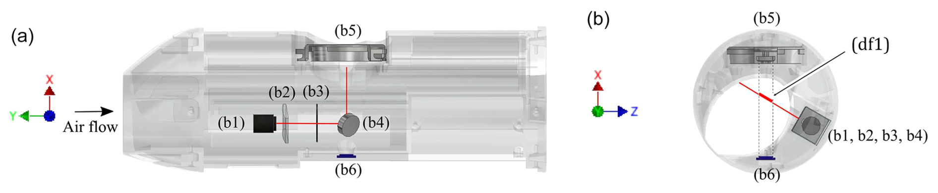
Figure 1 Design of the UCASS and arrangement of its optical elements. Panel (a) shows the side view of the UCASS, while panel (b) shows the front view. The definition of the particle detection zone (df1) has been added to the figure. Adapted from Smith et al. (2019).

Particles are counted, which pass through the instrument's optically sensitive region along the detection laser. The ratio of the scattered light generated by a penetrating particle is determined by means of two annular elements in the detector optics. This signal ratio is judged according to whether a detection event contributes an accepted count value or not. Based on scattered light intensity, the accepted counts are categorised into size classes (16 bins) using size-based look-up tables obtained by calibrations and based on Mie theory. Depending on the chemical composition of detected particles, different refractive indices must be considered, for example between 1.31 + 0j (water) and 1.52 + 0.002j (Saharan dust) (see Girdwood (2023) for further more specific details), whilst for Saharan dust other values are also found, e.g. 1.53–0.0015j (Kandler et al., 2007). Knowledge of the flow velocity and the dimensions of the sensing volume is required to determine accurate particle concentrations.

2.2 The thermal flow sensor (TFS)

The thermal flow sensor (TFS) model “FLW-122” for the gaseous media by B+B Thermo-Technik GmbH was used for this study. The TFS has a length of 6.9 mm, is 2.4 mm wide, and is 0.2 mm high (without electrical connections). The TFS surface consists of two platinum resistor elements, one of which is the heater and the other of which is the reference element. The heater is a small-sized low-resistance element (R_H (0 °C) = 45 Ω); the reference element (R_S (0 °C) = 1200 Ω) is of high electrical resistance. The two platinum resistors are interconnected and are adjusted via applied voltage to a specified temperature difference. The heat dissipation from the heater to the environment corresponds to the energy loss per unit of time, which in turn corresponds to the power P converted in the resistor.

The temperature of the heating resistor decreases with increasing rate of flow surrounding the TFS. As platinum is a PTC thermistor, the conductivity of the resistor increases as the temperature falls; hence the resistance of the heater decreases. To counteract this and to maintain the differential temperature between heater and reference, the voltage is increased. The higher the flow velocity, the higher the voltage (hereafter, signal voltage) required to maintain the temperature difference. According to the sensor data sheet (B+B-Thermo-Technik, 2016), the sensor's response sensitivity is 0.01 m s⁻¹ with an accuracy of better than 3 % and a temperature sensitivity of usually less than 0.1 % K⁻¹. The raw TFS data are recorded with a resolution of at least 4 Hz and then averaged to the common 1 Hz data basis. Thus, most important variabilities in the UCASS internal flow should be captured in sufficient resolution. In addition, low-frequency influences such as the pendulum motion (order of magnitude 0.1 Hz) and the rotation (of 1 Hz at most) of the balloon payload are also temporally resolved. Further detailed information on the TFSs (e.g. concerning the power and sensitivity of the implemented Z diode) may be found in the manufacturer's manual (B+B-Thermo-Technik, 2016).

For TFS calibrations, the following parameterisation, a modified form of King's law (Guellouz and Tavoularis, 1995), is often used:

$$\begin{array}{}\text{(1)}& U^{\mathrm{2}}=A+B\cdot v_{\mathrm{TFS}}^N,\end{array}$$

where A (in V²), B (in V² s m⁻¹), and N (dimensionless) are coefficients determined by calibrations; v_TFS is the flow velocity (in m s⁻¹); and U is the electrical output voltage (V). Rearrangement of Eq. (1) leads to the desired expression for the flow velocity (here v_TFS) as a function of measured voltage. King's law, a combination of the Nusselt number and Reynolds number (see Cardell, 1993, or Bearman, 1971), is primarily influenced by temperature fluctuations due to the temperature dependence of air's thermal conductivity and the dependence of the kinematic viscosity on the air density. Extensions of this equation by correction terms allow for considering changes in ambient temperature (see Cimbala and Park, 1990). On the one hand, these corrections apply to significantly warmer temperatures (300–307 K) than relevant to balloon soundings, and on the other hand, they require a set of temperature measurements, including the accurate temperature of the TFS surface itself. The TFS calibrations to assign a flow velocity to the output signal were carried out under laboratory conditions. To account for the dependence of the in-flight flow measurement on air density, a corresponding correction (dependent on static air pressures and ambient temperatures upon vertical sounding) is applied to measured data during post-flight analyses.

Based on the ideal gas law and on laboratory conditions during calibrations (p₀, T₀, and humidity expressed as virtual temperature), the correction $v_{\mathrm{TFS}}^{\mathrm{corr}}$ is obtained by multiplying v_TFS (according to Eq. 1) by a correction factor (at given ambient conditions p_amb, T_amb):

$$\begin{array}{}\text{(2)}& v_{\mathrm{TFS}}^{\mathrm{corr}}=v_{\mathrm{TFS}}{\displaystyle \frac{p_{\mathrm{0}}}{p_{\mathrm{amb}}}}\cdot {\displaystyle \frac{T_{\mathrm{vi}}}{T_{\mathrm{0}}}}.\end{array}$$

The virtual temperature T_vi was used instead of the ambient temperature T_amb. Hence, any change in the air's molar weight, the air's mass density, and heat capacity due to water vapour load is accounted for. As long as no phase conversion occurs, the temperature ratio also reflects the current moisture conditions in the atmosphere.

In addition, a cold-chamber test was carried out at various temperatures down to −20 °C (Supplement, Sect. S1) to investigate the sensitivity of the TFS system (particularly its electronic compounds) to significantly colder temperatures than those under laboratory conditions.

To mount the TFS on the UCASS, a 3D-printed polylactide case was produced. This was precisely adapted to the dimensions of the inner flow tube and the outer shape of the UCASS and extends the total length of the UCASS by a further 49 mm (cf. Fig. 2).

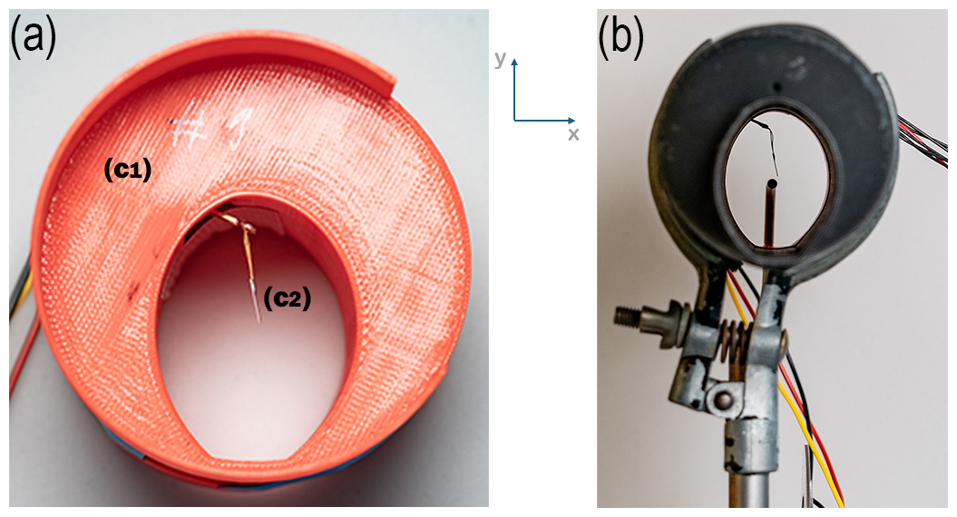
Figure 2 (a) The TFS housing (“c1”), which also contains the control and regulation electronics of the TFS. The sensitive area of the TFS with a length of 6.9 mm is labelled “c2”. (b) The frontal view of the experimental setup. The perspective is in the direction of flow towards the UCASS front and into the flow tube, looking at the TFS and the Prandtl Pitot tube, which is located downstream behind the TFS.

2.3 The Prandtl Pitot tube

The Prandtl Pitot tube (PPt) model “TSI 8710 plus” (re-calibrated in July 2022 for flow velocities of 1–10 m s⁻¹) by TSI Inc. was used as a reference instrument for calibrating the TFSs. Via the Pitot tube's entry, aligned against the direction of flow, the stagnation pressure (the sum of the dynamic and static pressure components) is measured. The outer tube of the Prandtl instrument with ring-shaped perforation allows for measuring the static pressure component. Conversion of Bernoulli's theorem to resolve the flow velocity leads to

$$\begin{array}{}\text{(3)}& v_{\mathrm{PPt}}=\sqrt{{\displaystyle \frac{\mathrm{2}\left(p-p_{\mathrm{stat}}\right)}{\mathit{\rho }}}},\end{array}$$

where p_stat is the static pressure (in hPa), ρ is the air's mass density (in kg m⁻³), v_PPt is the flow velocity (in m s⁻¹), and p is the stagnation pressure (in hPa). According to the PPt's calibration certificate, an uncertainty of generally less than 1.5 % (at 1 m s⁻¹) is to be expected, which decreases to ∼ 0.6 % at a flow velocity of 10 m s⁻¹.

2.4 The wind tunnel

The calibrations were conducted in the horizontal wind tunnel of the JGU Mainz. This facility (schematic in the Supplement, Fig. S3) has a total length of 4.6 m and a circular outlet opening of 0.64 m. The maximum achievable wind speed is approximately 20 m s⁻¹, generated by a 12-bladed impeller rotor in combination with a 14-bladed stator, both of which have an outer diameter of 0.8 m. The rotor hub (0.4 m in diameter) is encased by a tapered cone downstream of the stator to aerodynamically optimise the transition from the impeller housing (total length 1.25 m) to the flow channel (3.41 m length). The flow channel widens at 7° towards the horizontal over a horizontal distance of ∼ 2.0 m. In the area of the maximum channel diameter, a gauze and a honeycomb mesh with a total thickness of 0.1 m are installed to laminarise the flow. Further downstream, the flow channel diameter reduces via a radiused narrowing to compress the airflow. The channel's outlet with a constant diameter of 0.64 m extends over a distance of 0.35 m.

2.5 Calibration setup and procedures

Generally, all setups for the TFS calibration were placed centrally within the wind tunnel's laminar exit flow and in line with the tunnel's ring outlet edge to prevent potentially forming turbulence from affecting the calibration.

2.5.1 TFS–PPt interactions

For exploring whether an extension of the UCASS by the TFS housing (with installed TFS) causes a measurable impact on the flow at the position of the UCASS optical detection region, a 3D-printed replica of the UCASS housing was used. Holes were drilled into the housing replica at two different positions along its longitudinal axis in order to (1) place the PPt inlet at the position of the optical detection area within the flow tube and (2) place the PPt inlet inside the TFS housing at the TFS's position while replacing the TFS. The replica housing was lacking all optical elements (laser diode, mirrors, or photodiodes) that an operational UCASS comprises; all bulges along the flow tube's inner wall were evened out for this experiment.

Furthermore, a thermal anemometer (TA, by TSI Inc., model TSI 8455-300-1) was used to control the ambient flow generated by the wind tunnel. The TA was calibrated against the PPt in the free tunnel flow at flow velocities of 2–8 m s⁻¹. Then the experimental setup of the UCASS replica with integrated PPt was aligned iso-axially in the central flow of the wind tunnel. The experiments carried out are listed in Table 1.

Table 1 List of experiments (Exp.) conducted with the PPt at various positions inside the UCASS and TFS housing during wind tunnel flow calibrations.

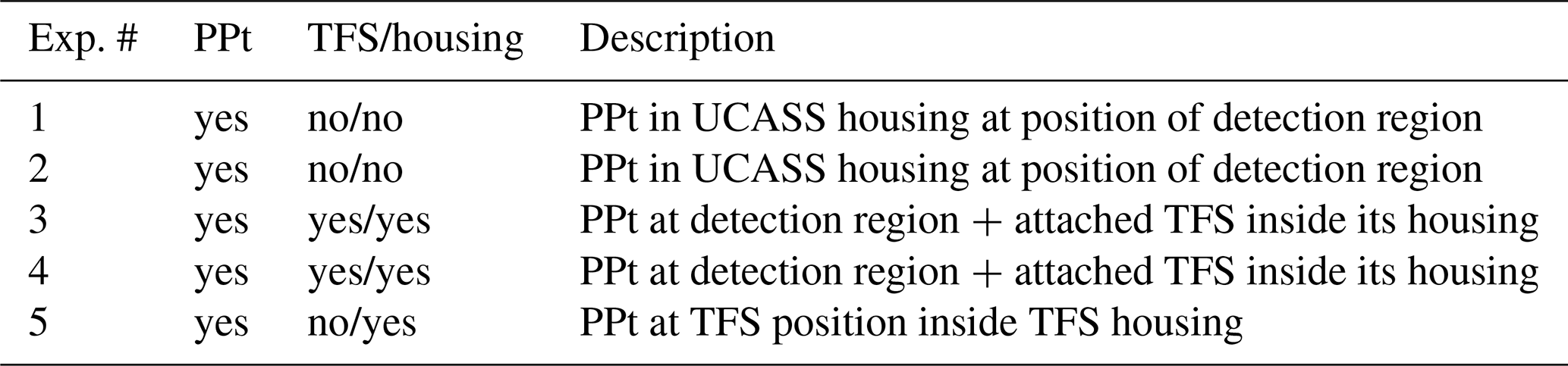
The experiments were conducted at ambient wind tunnel airflows of 2 ≤ v < 10 m s⁻¹ in increments of ∼ 1 m s⁻¹. 10 individual measurements were averaged for each of the seven different wind speeds. The results of these experiments are shown in Fig. S4 as correlations between TA-measured flow speeds (v_TA) and those from the PPt (v_PPt) within the UCASS flow tube. Notably, the UCASS tube flow velocity is generally increased compared to ambient wind speeds if the UCASS is iso-axially aligned with the ambient flow field, which was previously described by Smith et al. (2019) and confirmed during calibrations presented herein (see Sect. 3.2).

This experiment series demonstrates that applied modifications (extension of the flow tube geometry and implementation of the TFS) have hardly any measurable influence on the flow through a UCASS. At balloon ascent velocities, usually well below 10 m s⁻¹, none of the data series stood out from the statistical uncertainty. Therefore, the technical modification proposed herein is expected to have negligible impact on the measurement performance of the UCASS.

2.5.2 Cross-sectional flow profile

For the following, a TFS housing shell without an installed TFS was mounted on a UCASS to exclude any obstacle to the airstream through the flow tube. The PPt was attached near the outlet of the TFS housing so that the PPt inlet was iso-axially aligned and positioned as far as possible inside the flow tube along the longitudinal axis of the UCASS. Thus, along the setup's longitudinal axis, the PPt inlet was located at the point where the TFS would normally reside. The PPt was moved perpendicularly to the flow and in small increments (∼ 1–2 mm) along a line between the two extremes of the flow tube's elliptical cross-section. The flow speed in the wind tunnel was kept constant, and for a single data point, the average of 15 velocity measurements was taken at each PPt position. The profile measurements of the tube flow profile were carried out for tunnel wind speeds of about 5 and 7 m s⁻¹.

Figure 3 shows the corresponding results. The maximum standard deviation in the PPt's position is estimated to be 0.2 mm and is shown together with the maximum standard deviation of the PPt data obtained from this series of measurements (σ_max = 0.05 m s⁻¹) in the bold-framed box. The position where the TFS would be aligned (if – except for this experiment – installed and adjusted by means of a positioning device) is marked by the grey-shaded area in Fig. 3. The flow profiles exhibit asymmetry. The boundary layer at the positive end of the y axis seems broader than at its negative end. The reason for this is most likely the quasi-elliptic but asymmetric flow tube cross-section of the UCASS flow tube. As the ambient flow increases, an increased boundary layer thickness is visible in the UCASS internal flow profile. Moreover, the flattening of the flow profile is clearly visible towards the centre of the flow tube. For typical UCASS flow rates (here ∼ 2–10 m s⁻¹), this demonstrates that at the intended installation position (grey shaded area), the TFS flow measurement occurs in the free tube flow of the UCASS. Notably, the determined cross-sectional profile applies to a straight-line flow (i.e. the AOA equals zero). Under variable AOAs (see Sect. 2.5.4) and at the selected TFS position, any wall effects still have the least influence on the TFS measurement compared to other positions along the tube's cross-section.

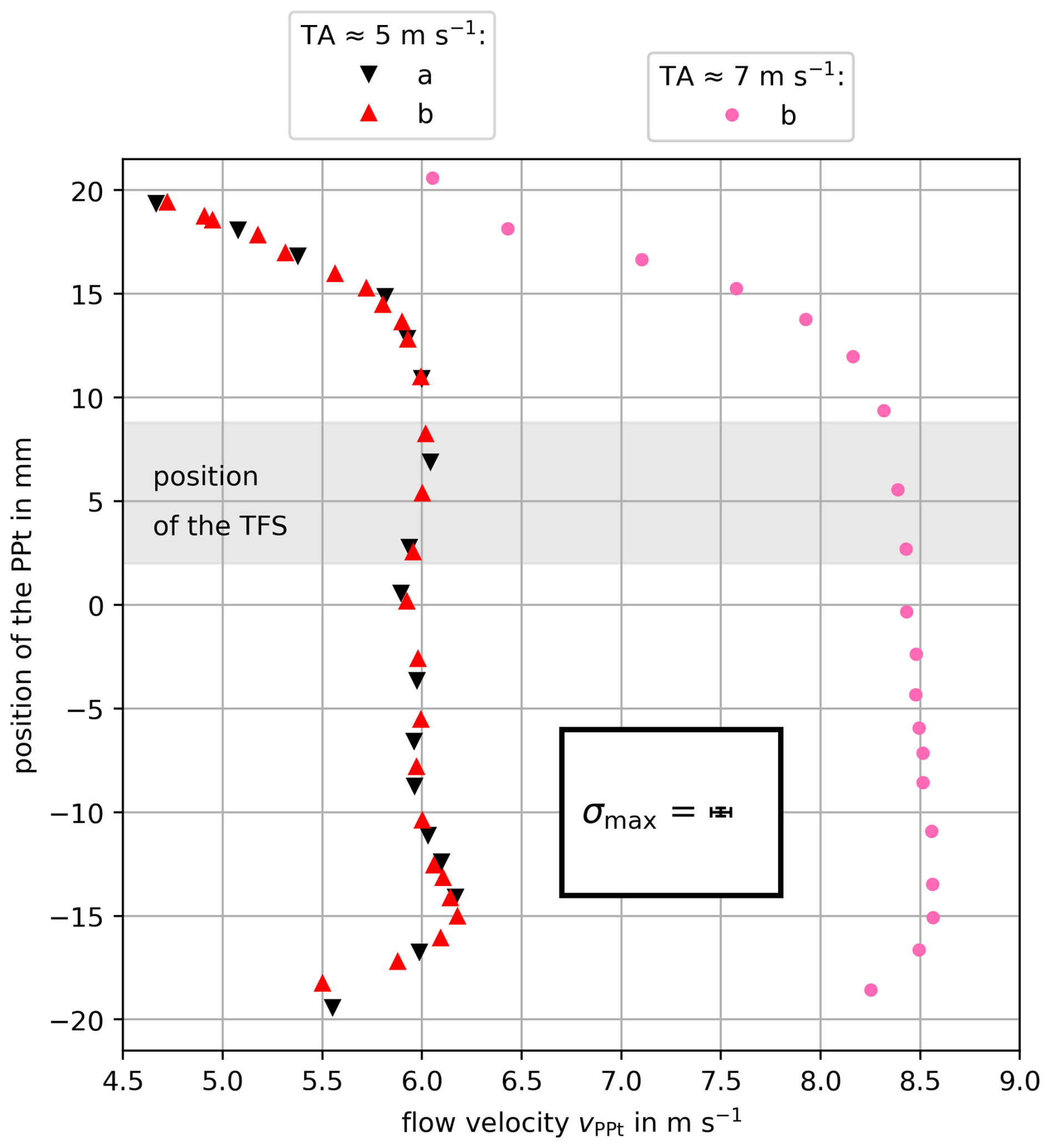
Figure 3 Resulting flow velocity profiles along the elliptical cross-section of the instrument's flow of the UCASS or of the TFS housing with a diameter of 40 mm × 30 mm (length × width). Along the cross-section's main axis, the flow velocity measurements were carried out; twice for an ambient flow velocity of ∼ 5 m s⁻¹ (forwards “a” and backwards “b”, respectively) and once for ∼ 7 m s⁻¹ (direction “b” only). Each data point represents an average of 15 velocity measurements. The error bars, which are shown representatively in the bold-framed box, show the maximum standard deviation for PPt's position (σ_max = 0.2 mm) and for all flow velocities measured with the PPt (σ_max = 0.05 m s⁻¹). The position of the TFS (if installed) is marked by the grey area.

2.5.3 Iso-axial flow calibrations

With the iso-axially aligned setup (see beginning of Sect. 2.5) and with the PPt inserted from the rear into the UCASS–TFS housing, such that the PPt inlet is positioned close to the TFS (cf. Sect. 2.5.2 and Fig. 2b), the flow calibrations were performed. The TA installed in the free wind tunnel flow (outside the UCASS housing; see Sect. 2.5.1) was used to control the ambient flow speed.

The TFS calibration comprised a series of measurements at different flow velocities. From slightly more than 0 m s⁻¹, stepwise increasing flow velocities were set in the wind tunnel until ∼ 10 m s⁻¹ was reached. About 25 measured values were recorded for the calibration of a single TFS. As disturbance-related fluctuations occurred in the measured values during the calibration of both the PPt and the TFS, 15 measured values were recorded for each of the sensors at each ambient flow speed set. Mean values and standard deviations were determined from these PPt and TFS data. Each TFS was calibrated individually, and the results of these calibration series are summarised in Sect. 3.1 to 3.4 (see also Sects. S2 and S3 in the Supplement). After changing the TFS, the iso-axial and centred alignment of the experiment setup at the wind tunnel outlet was frequently checked and readjusted if necessary.

2.5.4 Flow calibrations under variable AOAs

For balloon soundings, the payload (incl. UCASS) is usually attached approx. 60 m (via unwinder, model “UW1” by Graw GmbH & Co. KG) below the balloon on a cord. The long cord is intended to dampen the pendulum motion of the payload. Due to the vertical offset between the balloon and the payload, also a horizontal offset between both balloon and payload occurs depending on the horizontal wind speed. The balloon may lead the payload by a certain horizontal distance, unless the horizontal wind speed is zero. Hence, during the balloon's ascent and with horizontal winds the UCASS is likely inclined at a certain angle relative to the direction of vertical lift. In addition, pendulum motion and rotations of the payload during flight cannot be completely prevented, which can lead to a variable alignment of the UCASS relative to a straight ascent due to several superimposed effects. Therefore, the impact of inclinations of the UCASS with respect to the direction of flow on (1) the TFS calibration and (2) on the flow velocity within the UCASS is to be quantified.

The experimental setup was aligned and positioned as described previously (beginning of Sect. 2.5). The iso-axial alignment corresponds to the zero position (φ = 0°, ϑ = 0°). As the UCASS flow tube is mirror-symmetrical along the vertical axis, the UCASS was horizontally inclined only along the positive x axis (φ) for changing AOA. Due to the quasi-elliptical shape of the UCASS flow tube, the effects of the flow angle in the y direction (ϑ) were analysed for both the positive (UCASS inlet points upwards) and the negative (UCASS inlet points downwards) deviation from zero. Figure 4 illustrates the measurement setup and provides an example of the angular distribution under which the UCASS was aligned relative to the ambient flow field. Note that the frame for holding the UCASS–TFS setup also fixes the PPt (marked in Fig. 4a), which remains aligned with the UCASS longitudinal axis and is positioned as close as possible at the TFS. Any angular change in the flow direction to the UCASS inlet therefore affects the entire assembly (cf. Fig. 4c). At the beginning of each measurement series, data were recorded for five different ambient flow speeds in the zero position (0°, 0°) to verify the calibration curve of respective TFS used. The angles were then set within the angle grid shown in Fig. 4b. 15 measured values of the PPt and the TFS were recorded for five different tunnel flow speeds between about 3 and 7 m s⁻¹ and the mean value with standard deviation were determined from PPt and TFS data. The results are summarised in Sect. 3.3. An attempt was made to reproduce the set tunnel flow velocities for each measurement series at varied AOA, which allowed also for investigating the relationship between the flow velocities outside and inside the UCASS housing at variable AOAs (see Sect. 3.4).

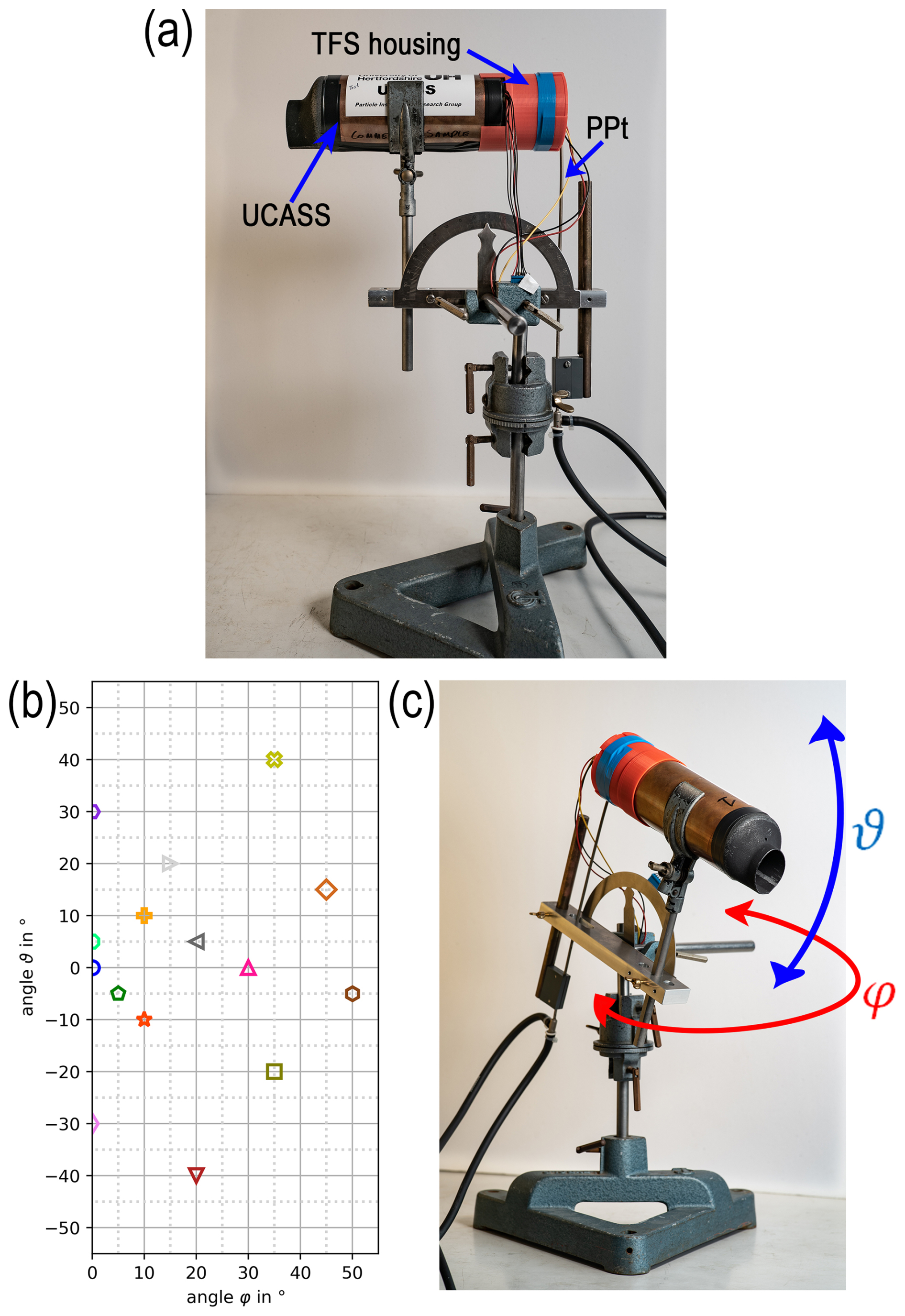
Figure 4 Measuring setup with UCASS, mounted TFS housing, and installed PPt (from the rear reaching into the TFS housing), fixed in a vertically and horizontally tiltable apparatus with scales for reading the deviation angles in each direction. (a) Side view in horizontal orientation. (b) Variable deviation angles, which were set in angular degrees deviating from the zero position (iso-axial case) during the experiments. (c) View of the measuring setup under horizontal and vertical displacement from the zero position.

2.6 UCASS internal flow estimates

Besides the counted and classified particles, UCASS also records the particles' average beam transit times (named MToF, mean time of flight) in four different size ranges. In principle, these beam transit times could be used to estimate the flow speed in the measurement volume and therefore would provide another option for a sampling volume assessment. Such an approach is used for example in connection with the particle detectors by Alphasense OPC-N2 and OPC-N3 (Bezantakos et al., 2020). We therefore correlated the measured TFS velocities with the inverse of the different MToF values reported for each interval, when particles were detected. A considerable number of apparently clipped values (piling at the apparent bottom and top end of the measurement scale) were removed. Still, while there was a very weak correlation found between the inverse MToF and the TFS, the huge variations, the clipped values and the scarcity of data – in most 0.5 s intervals no particles are detected – prevent this approach from being used as a measurement for a flow rate in UCASS.

3 Calibration results

To this point, it has been demonstrated that

1. the insertion of the TFS into the flow tube of the UCASS has no measurable impact on its particle-sensitive area (Sect. 2.5.1) and

2. as the TFS installation is achieved using a positioning device it is systematic for all TFSs used whose measurements occur outside the tube's boundary layer in the central UCASS flow.

Hence, the assumption seems appropriate that integrating TFSs into the UCASS flow tube did not generate any additional interferences for the calibrations discussed hereinafter.

3.1 High-resolution calibration (HRC) and three-point calibration (TPC) of the TFS

According to the functional relationship described in Eq. (1), the measured TFS output voltage is calibrated versus the PPt-measured flow velocity, which is used hereafter as the calibration curve of a TFS (further details in Sect. S2 in the Supplement). For each measuring point, the mean value plus (minus) the associated standard deviation – i.e. the extremes of variability – was inserted into the calibration curve function, yielding a deviation from the averaged measurement point of not more than 0.08 m s⁻¹, which corresponds to a percentage maximum of 1.3 %. The results show that the different TFSs exhibit very similar behaviour and that the parameterisation of the calibration curve function is valid for all calibrated TFSs. Table S1 (see Supplement) lists the parameterisation coefficients for the TFSs analysed in the calibration results. Repeated calibration series with a larger time offset and with the same TFS after disassembly/reassembly of the setup also reproduced previous values within 1.8 % at a maximum and on average within 1 %, in the relevant range of ambient flows. However, the measurements of the calibration curves were likely influenced by the ambient temperature and pressure conditions in the laboratory as both affect air's mass density, which in turn controls the heat advection at the TFS.

In the process of these high-resolution calibrations (calibrations with up to 25 data points and in the following denoted by HRC) and analyses of the calibration curves, it was found that only three calibration points (at ∼ 2, 5, 8 m s⁻¹) reproduce the calibration curve with acceptable accuracy (see Supplement, Sect. S2, for details). For the TFS used (here, TFS 8), and at tunnel flow speeds between 2 and 8 m s⁻¹, the three-point calibration (in the following denoted by TPC) curves did not deviate by more than 1 % from the highly resolved initial calibration curve.

3.2 Internal versus external flow velocity

The PPt was repositioned next to and slightly upstream of the UCASS inlet to measure in the free flow of the wind tunnel (setup is shown in Fig. S5). The UCASS-integrated TFS 8 had previously been calibrated with the PPt to have a calibration curve (TFS 8.2 (TPC) see Table S1) under the same laboratory conditions as the experiment. The UCASS was aligned iso-axially to the ambient flow of the wind tunnel and centred at the annular outlet of the tunnel. The wind tunnel flows were stepwise increased from slightly more than 0 to up to 11 m s⁻¹ and then decreased with a total of 17 different settings. For each of the ambient flow speeds, 15 velocity values were recorded as measured by the PPt to be averaged. In Fig. S6, the PPt-measured flow velocity outside the UCASS is displayed in reference to the UCASS internal flow velocity determined with the TFS 8. The velocity range relevant to balloon soundings (2–8 m s⁻¹) is indicated by the black dashed square.

Within this range, 10 different values of ambient flow speed were set for each measurement of this series. The standard deviation σ of the PPt data ranges between 0.01 and 0.04 m s⁻¹. Only the mean value of the TFS output voltage was noted, which resulted from the automated averaging by the multimeter used. During the TFS 8 calibrations, standard deviations of at most 0.08 m s⁻¹ were obtained corresponding to a maximum relative deviation of 1.3 % (extremes of variability; cf. first paragraph in Sect. 3.1). A first-order polynomial fit was created for the recorded measurement. The resulting line fit indicates that in an iso-axial arrangement, the UCASS internal flow velocity exceeds the outside flow speed. Calculated from 10 data points at external wind velocities between 2 and 8 m s⁻¹, the UCASS internal flow velocity is increased by 10.7 %–11.9 %, with an average relative deviation of 11.3 %, as compared to the external flow speed.

This result quantitatively compares well with the results of Smith et al. (2019), who simulated an increase in the UCASS internal flow velocity by 12 % under an iso-axial alignment of the UCASS and at an ambient flow speed of 5 m s⁻¹. Taking into account the standard deviations of averaged data points determined here may put the small deviation between previous and current results into perspective.

However, in balloon-borne UCASS field applications, the balloon ascent rate is usually used to determine the sample volume flow and thus the measured particle number concentrations (e.g. Kezoudi et al., 2021). So, when a UCASS was iso-axially aligned during a straight balloon ascent at rates of 2 to 8 m s⁻¹, the GPS or pressure-based calculation would lead to an underestimated UCASS sample volume flow by about 11 %–12 % and the particle number concentrations would be overestimated accordingly. Therefore, from the current point, a direct measurement of the UCASS internal flow velocity during flight appears useful, but as will be shown (Sect. 4), the conditions during balloon soundings are more complex and the necessity for a flow velocity detector integrated into the UCASS becomes all the more obvious.

3.3 UCASS internal flow velocity under variable AOAs

Compared to previous experiment series, the UCASS was deliberately offset from the iso-axial orientation (cf. Sect. 2.5.4).

Figure 5 shows the highly resolved calibration curve of TFS 8. The mean values from experiment series at five ambient flow speeds are also depicted for each AOA. The standard deviations are not shown for the sake of clarity of the figure. The error in setting the UCASS deflection angle was estimated to be ±0.5° in each case. In the zero position (0, 0°), which was calibrated once at the beginning and at the end of the series, the σ values ranged between 0.002 and 0.003 V (TFS 8 output voltage) or between 0.02 and 0.04 m s⁻¹ (PPt). With increasing AOA, the standard deviations (σ) rose to a maximum of 0.025 V (TFS 8) and 0.09 m s⁻¹ (PPt). Hence, the fluctuations in measured variables generally increased with increasing AOA.

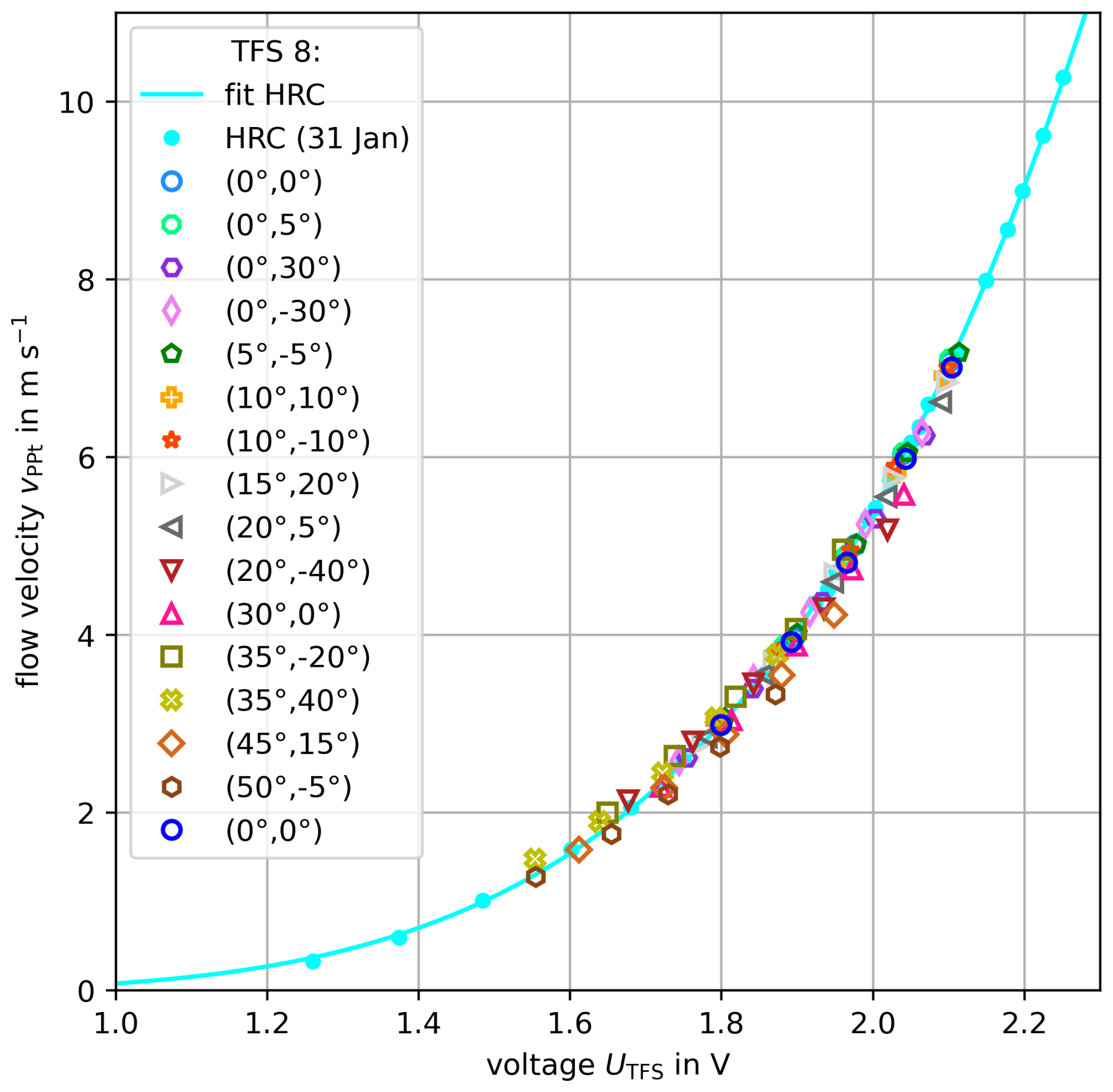
Figure 5 Comparison of the high-resolution calibration (HRC) curve with measurements of the UCASS-implemented TFS 8 at variable angles of attack. The standard deviations of individual data points are not shown for the sake of clarity.

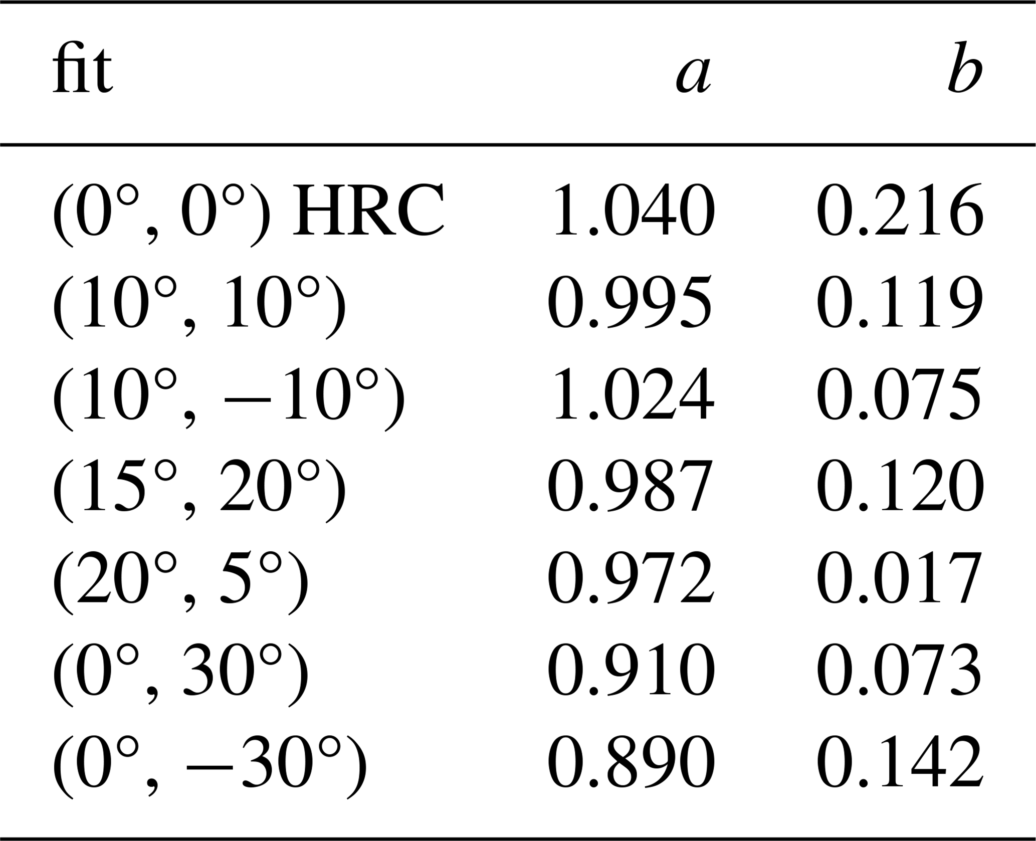
Table 2 Parameters of the linear fit function ($v_{\mathrm{PPt}}=a\cdot v_{\mathrm{TA}}+b$) to selected UCASS internal flow velocities measured under variable angles of attack (AOAs) in reference to the main wind tunnel flow speed.

Based on the TFS 8 calibration curve, the flow velocities $v_{\mathrm{TFS}}^a\left(U\right)$ were determined with the mean TFS output voltage values ($\overline{U}$). These are compared with the flow velocities $v_{\mathrm{TFS}}^b\left(U\right)$ resulting from the extreme values of standard deviation at each mean output voltage (i.e. $\overline{U}\pm \mathit{\sigma }$). The maximum standard deviation range observed was ±0.31 m s⁻¹ (8.3 %). Oscilloscope records of the variations in the TFS output voltage over 20 s clearly indicated an increasing scatter intensity when varying the AOA of UCASS, e.g. from (0°, 0°) to (20°, −40°). The output voltage fluctuations were invariant in time (in particular non-periodic) and stationary, i.e. of a rather statistical nature.

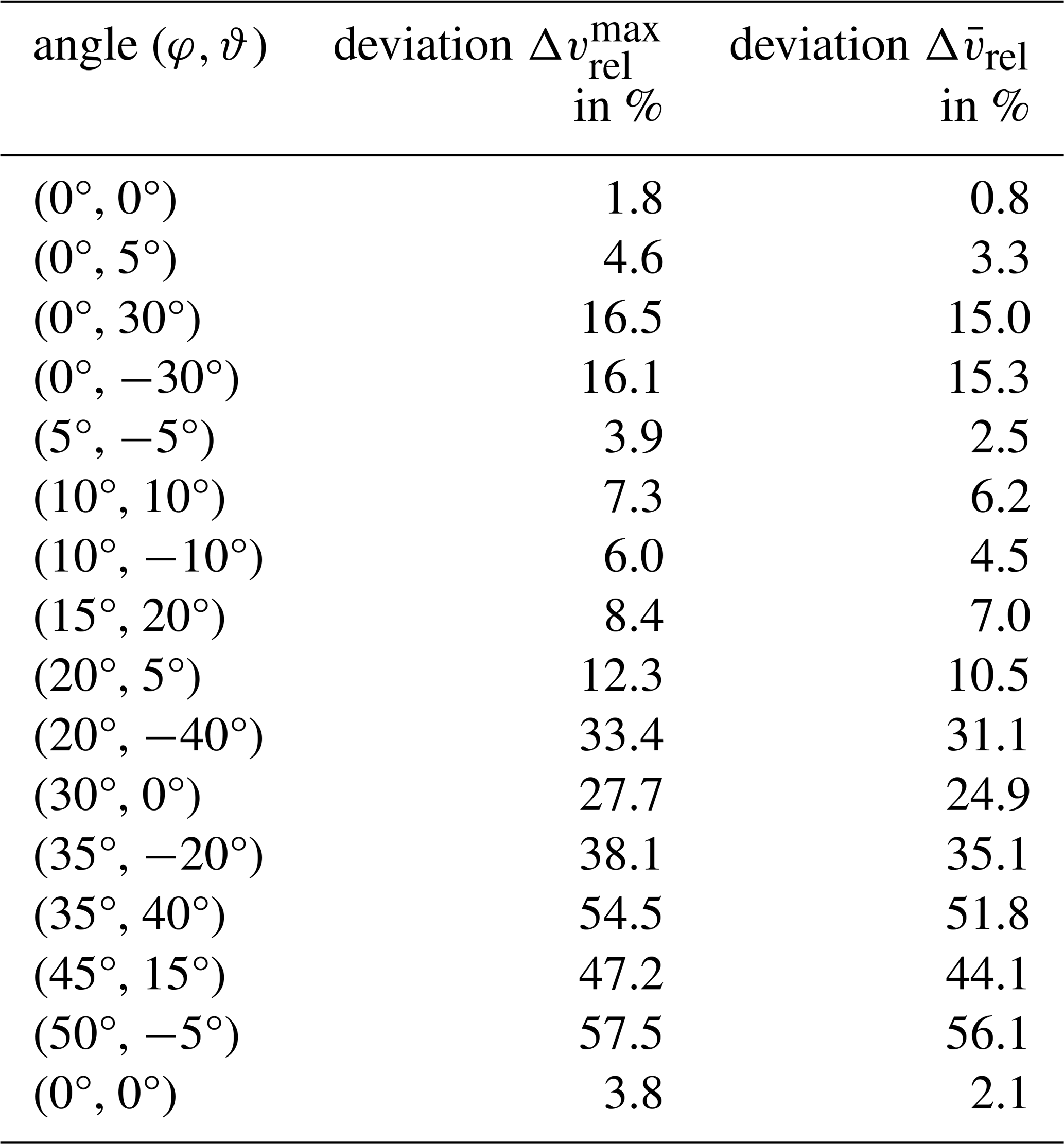
The mean values of the TFS measurements were inserted into the calibration curve function of TFS 8 to determine the flow velocities (v_TFS) to be juxtaposed with the mean PPt-measured flow velocities (v_PPt). The flow velocity determined with the calibration curve was used as the reference, and the error is considered with

$$\begin{array}{}\text{(4)}& \mathit{\epsilon }={\displaystyle \frac{v_{\mathrm{TFS}-}{v}_{\mathrm{PPt}}}{v_{\mathrm{TFS}}}}\cdot \mathrm{100},\end{array}$$

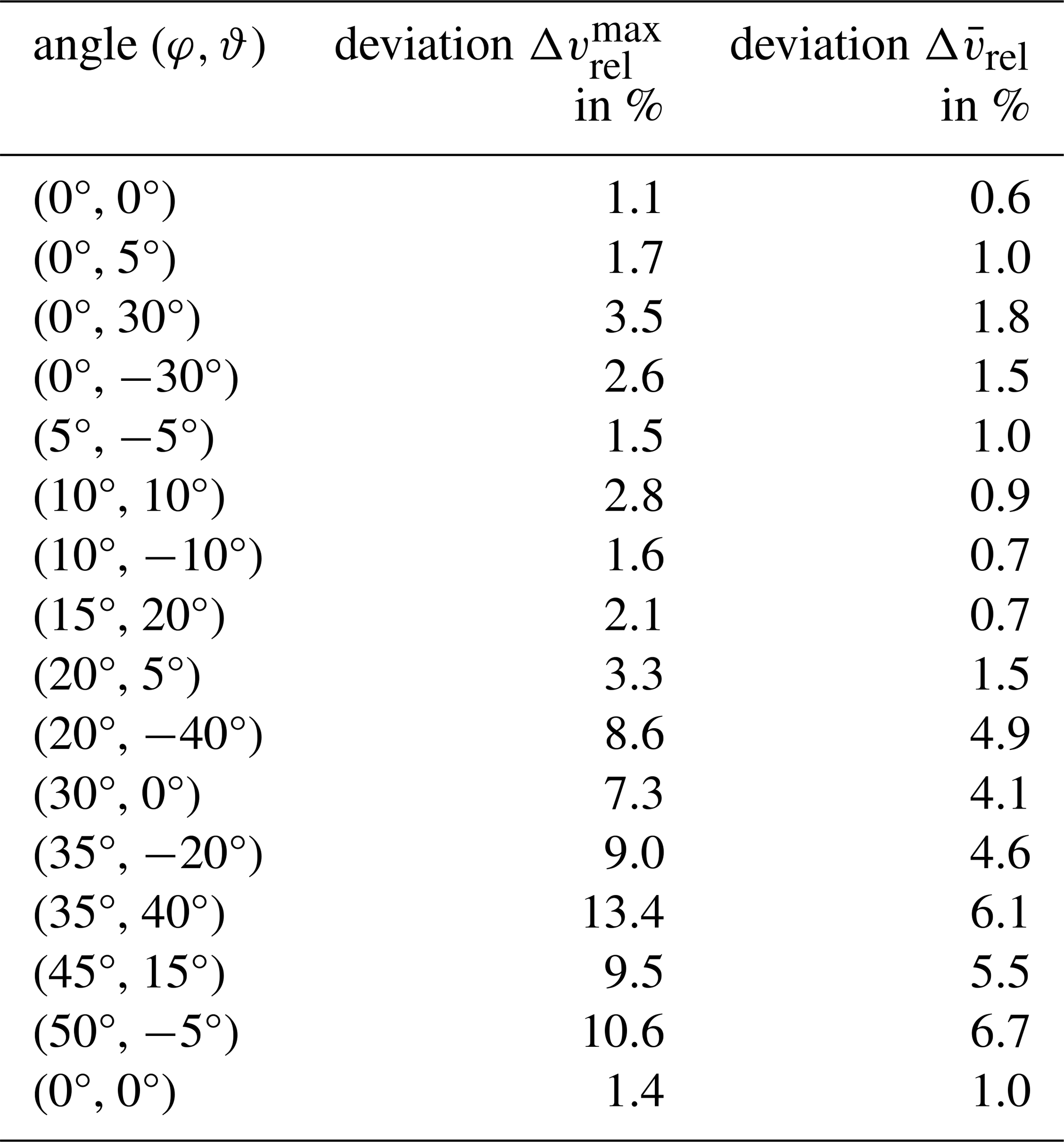
out of which the maximum percentage error and its mean resulted for each AOA. Table 3 shows the maximum and the mean of the relative percentage deviation of measured values at variable AOAs compared to the calibration curve of TFS 8. At AOAs of up to 30°, the maximum relative percentage deviation was 3.5 %, and above 30°, the relative percentage deviation of measured values from the calibration curve increased significantly. At such large AOAs, the σ of TFS-measured voltages also rose substantially. During balloon sounding, UCASS inclinations of more than 30° from the vertical are not expected. In an earlier study (Smith et al., 2019), a model was used to simulate the angular inclination of the UCASS in relation to the direction of ascent. Initial pendulum oscillations of up to ±20° were assumed, which were damped to around ±5° within about 30 s. If these conditions occurred at an actual balloon sounding with UCASS, the percentage relative deviation of measured velocities as determined here (based on the TFS 8 calibration curve) would be a maximum of 2.8 % under variable AOAs smaller than 20°. Hence, even at UCASS inclinations of up to 20°, the particle concentration is affected by this angle deflection with a maximum uncertainty of less than 3 % (maximum relative deviation). To validate the TFS 8 data series, the measurements were repeated with TFS 7 in the same setup. Corresponding results are summarised in Sect. S3 (Supplement), representing a qualitative and largely quantitative confirmation of the results and conclusions made.

Table 3 Maximum ($\mathrm{\Delta }{v}_{\mathrm{rel}}^{\max }$) and mean values ($\mathrm{\Delta }{\overline{v}}_{\mathrm{rel}}$) of the percentual relative deviation of measured flow velocities under variable angles of attack (AOA) for the calibration curve of TFS 8 (cf. Fig. 5).

3.4 Internal versus external flow velocity under variable AOAs

In Fig. 6, the velocity of TA-measured ambient wind tunnel flows (as reference) is plotted against the PPt-measured flow velocity inside UCASS. Standard deviations of 0.01 to 0.10 m s⁻¹ were determined for the ambient flow velocity between 2 and 8 m s⁻¹. For PPt data, σ values ranged from 0.02 to 0.09 m s⁻¹, which increased with rising ambient flow velocities and AOAs. With increasing AOA, the UCASS internal flow velocity decreased. For AOAs of (0°, 30°) and (0°, −30°) and beyond, the UCASS internal flow was slower compared to external flow velocities.

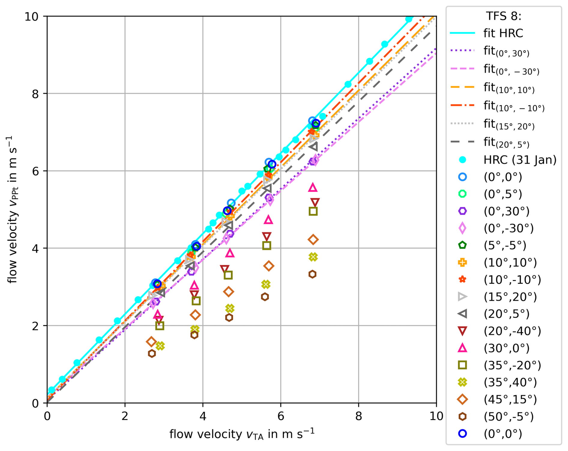
Figure 6 Comparison of the recorded flow velocities outside (v_TA) and inside (v_PPt) the UCASS at variable angles of attack during the series of measurements with TFS 8. The standard deviations (at the most ±0.1 m s⁻¹ at tunnel wind speeds between 2 and 8 m s⁻¹) are not shown for reasons of clarity. First-order polynomial fits were created for the flow velocities recorded under various angles of attack to compare with the high-resolution calibration (HRC) at the zero position (0°, 0°).

The UCASS internal flows in the zero position (0°, 0°) were used as reference and parameterised by a first-order polynomial fit. The comparison of (a) the calculated flow velocity inside the iso-axially aligned UCASS with (b) its internal flow velocities at AOAs of (0°, 30°) and (0°, −30°) revealed a relative percentage decrease in the flow velocity of around 15 % (see Table 4). For an iso-axially aligned UCASS, the internal flow is accelerated by ∼ 11.3 % on average (see Sect. 3.2). The contrary effects of (a) a flow acceleration inside the iso-axially aligned UCASS and (b) the deceleration inside the UCASS when deflected from the zero position are likely superimposed. Thus, with a UCASS inclination of 30° during a balloon sounding, the UCASS internal flow velocity is reduced by around 4 % net compared to the external flow. In turn, at such a UCASS inclination, a particle number concentration calculated with the GPS or pressure-based ascent velocities underestimates the prevailing trace material concentrations by only about 4 % under these conditions.

Table 4 Maximum ($\mathrm{\Delta }{v}_{\mathrm{rel}}^{\max }$) and mean relative deviation ($\mathrm{\Delta }{\overline{v}}_{\mathrm{rel}}$) of in-UCASS-measured flow velocity versus the wind tunnel flow speed as a function of the UCASS's angle of attack (AOA) in reference to the velocity ratio in the zero position (in correspondence to measurements shown in Fig. 6).

At a certain deflection angle (30°, 0°), a noticeable but undeterminable interference effect appears to have impacted the laboratory experiments. With increased deflection of the UCASS, the inlet opening of the UCASS is shifted out of the central wind tunnel flow and towards the tunnel's wall. With decreasing distance to the wall of the wind tunnel, effects of flow disturbances cannot be ruled out, which could influence the relative deviation from the calibration curve. Potentially, signal fluctuations are also amplified by flow disturbances that occur at the leading edge of the UCASS entrance when the UCASS is deflected too far from the zero-position. The TFS appears to be sensitive to such fluctuations. In addition, an influence of wind gusts on the experiment cannot be excluded, as the wind tunnel is operated inside a building but has connections to the building's exterior to enable enhanced wind tunnel flows.

4 Ambient measurements

Ambient balloon soundings were carried out with two UCASS instruments, such that two TFSs were operated in parallel during the respective ascents. The balloons' ascent rate is determined from both the static pressure measurements (v_p) and the GPS data, each of which are recorded independently. The static pressure in flight, resolved at 1 Hz, is converted to barometric altitudes by the internal primary data processing in the VAISALA sounding system, as recalculations (based on Sonntag, 1994) confirm. GPS and pressure-derived ascent rates correlate very well (regression yields a slope of 1 and a constant element of −0.1 m s⁻¹ with a coefficient of determination r² of 0.99).

4.1 Vertical profiles

Figure 7 shows vertical profiles of three balloon soundings launched from Tailfingen (Germany), at ∼ 900 m above sea level (a.s.l.) in August 2023. The profiles allow for comparing (1) the balloon ascent rate from the GPS measurements v_GPS, (2) the balloon ascent velocity from the static pressure measurements v_p, and (3) the flow velocities through the two UCASS units (TFS 1 and TFS 2) operated on each ascent. Results from other balloon soundings are shown in the Supplement (Fig. S10). The TFSs used for the balloon soundings and their calibration coefficients are listed in Table S3. The profiles are limited to an altitude of 7.5 km a.s.l., as at about this height the ambient temperatures fell below the specified temperature limit (253 K; see B+B-Thermo-Technik, 2016). Further laboratory tests are required to confirm the robustness of the TFS measurements also at temperatures of 253–220 K or to reveal the need for further corrections. As nearly all UCASS particle measurements were detected below 7.5 km, the restricted height range nevertheless covers the relevant part of the flight. The data are low-pass-filtered by a 10 s running average.

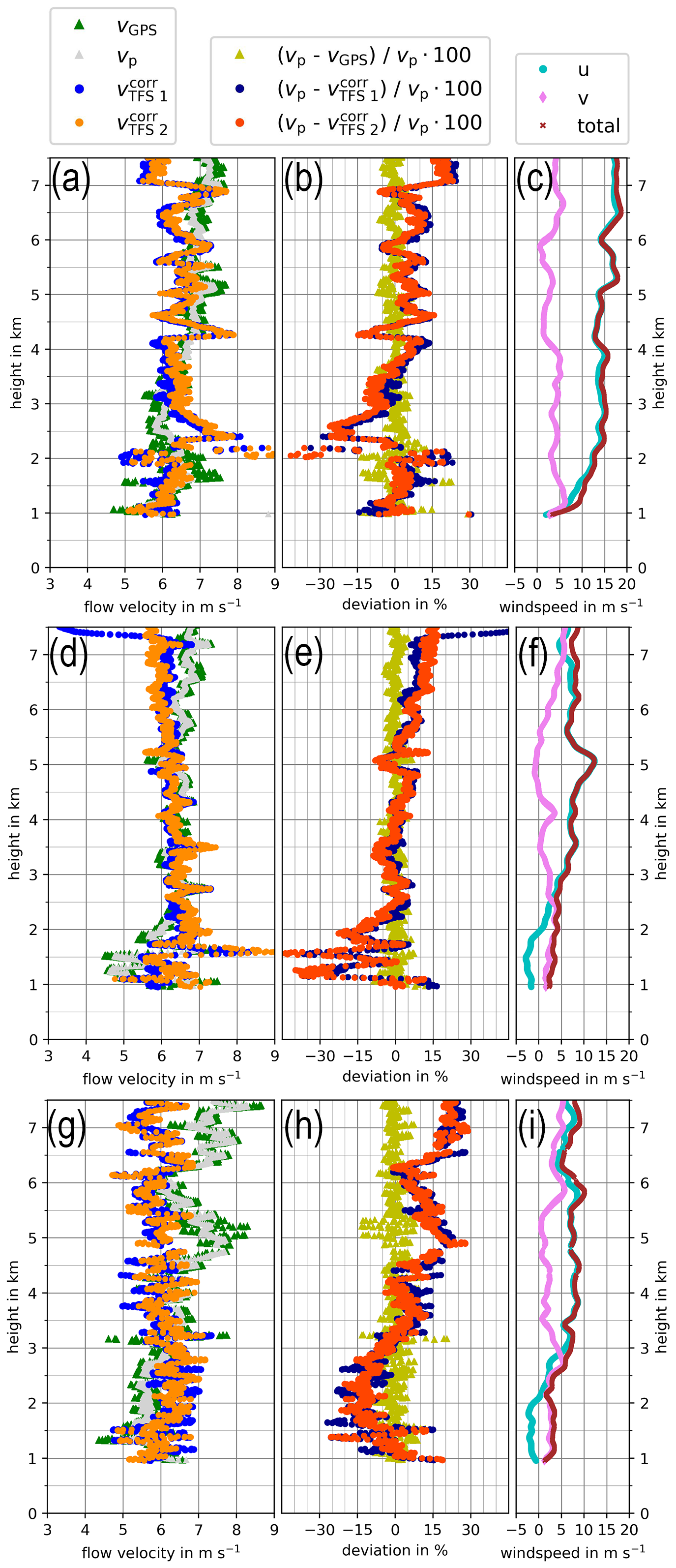
Figure 7 Vertical profiles of the vertical velocity based on measurements of changed GPS and barometric altitudes per unit time (i.e. v_GPS and v_p) and on TFS measurements of the flow velocity ($v_{\mathrm{TFS}}^{\mathrm{corr}}$) through the UCASS of selected balloon soundings during a field mission together with observed horizontal wind data (u and v) and the total wind speed (u+v) (a–c) from 12 August, launch at 14:10 (LT); (d–f) from 16 August, launch at 11:51 (LT); and (g–i) from 16 August, launch at 13:41 (LT). 10 s running averages of the respective data are shown. Additionally, respective deviations of the differently obtained flow velocities from each other are shown for each vertical profile (b, e, h). Note that the deviation of the ascent rates (i.e. the external flow velocity, GPS or p-based) in reference to the UCASS internal flow speed differs from zero over large parts of depicted flight sections. Occasional correlations of changing velocity ratios with changes in wind speeds are recognisable, but a general causality cannot be identified.

A common feature of the vertical profiles is the stronger scatter of the GPS-derived ascent rates compared to those based on pressure measurements. This might be connected to a larger uncertainty inherent in GPS. In general, however, both values are well-correlated. Up to ∼ 2 km of the balloon sounding of 12 August (Fig. 7a), the TFS measurements agree relatively well with GPS and the pressure data (see also Fig. 7b). Below ∼ 3 km, TFS 1 and TFS 2 deviate from the pressure and GPS data by up to 30 %. Up to ∼ 3.8 km, the different speed measurements from all instruments are comparatively consistent. Above 3.8 km, the TFS measurements (again consistent between TFS 1 and TFS 2) show periodically fluctuating and lower flow speeds (by up to 15 % and above 7 km altitude by up to 25 %) compared to those resulting from GPS and pressure.

During the earlier balloon sounding of 16 August (Fig. 7d) and up to an altitude of ∼ 2.4 km, the TFS-based velocities are systematically higher (in peaks by up to 45 %; cf. Fig. 7e) than corresponding values from GPS and pressure. In contrast to the previous case, the measurements of the four sensors are quite consistent at altitudes between 2.4 and 5.3 km, with deviations of seldom more than ±10 %. Above ∼ 5.3 km, the two independent TFS measurements, which correlate quite well with each other, both deviate increasingly from the GPS and barometric data with increasing altitude and show up to 15 % lower UCASS flows compared to the balloon ascent rates.

The balloon sounding on the afternoon of 16 August (Fig. 7g) shows a more or less satisfactory match between all four independent measurements only at the lowest altitudes (up to ∼ 1.3 km). Between 1.3 and 2.7 km, the TFS velocities are generally higher (on average by 15 %, in peaks up to 25 %; cf. Fig. 7h) than those derived from GPS and pressure. Above 3.2 km, reversely, the ascent velocities from pressure and GPS slightly exceed the TFS data. At altitudes of 4.5–5.5 km and above ∼ 6.2 km, GPS and pressure measurements commonly reveal increased vertical velocities that rise from about 6 m s⁻¹ to about 8 m s⁻¹. Within these layers TFS velocities are mostly 15 % (in peaks up to 25 %) slower than the ambient airflow. The origin of these features in the GPS and pressure-based velocity profile apparently has, if any, only a minor impact on the TFS measurements.

These examples suggest that over large parts of the vertical sounding (up to 7.5 km altitude), the flow velocity within the UCASS (and thus through its optically sensitive particle detection region) does not match the GPS or p-derived ambient flow velocity. For each of the vertical soundings shown in Fig. 7, the speeds of the horizontal wind components (u and v) and the sum of both as the total wind speed are also displayed in vertical profiles (Fig. 7c, f, i). Occasionally, changing wind speeds appear to be reflected in changing velocity ratios (e.g. the decrease in u at 4 and 6 km in Fig. 7c or the features in u at 5 km in Fig. 7f and at ∼ 6 km in Fig. 7i), which would indicate a certain correlation. However, a general causality between changing wind speeds and the ratio of TFS-based to p-based flow velocities through the UCASSs cannot be inferred without knowledge of the actually resulting AOA at which the UCASSs are sampling. Besides wind speeds, stability (Brunt–Väisälä frequency N²), turbulence (Richardson number, Ri), and wind shear as a function of altitude (not shown herein) were also investigated concerning their potential relationship with the variable velocity ratios, but no relationships of general validity could be identified.

4.2 Implications of observed features

Influences on the UCASS internal flow speed and pattern due to an additional installation of a TFS in a housing extension, if any, are negligible (Sect. 2.5.1). The sensitive area of the implemented TFS is located within the free tube flow through a UCASS, i.e. outside the boundary layer of the UCASS flow tube's inner walls (Sect. 2.5.2). Moreover, with an iso-axial alignment of the UCASS, the inner flow is accelerated by ∼ 11.3 % when compared to the ambient flow velocity around the UCASS (Sect. 3.2), which is in general agreement with earlier findings (Smith et al., 2019). As discussed in Sect. 3.4, with increasing angular deflection of the UCASS from the iso-axial orientation, the flow velocity inside a UCASS is decelerated towards values of the ambient flow speed and below.

The payload as used during the field mission had a total weight of up to 3.9 kg. About 10 000 L of helium is required for the balloon to yield enough buoyancy for the desired lift. Under conditions with horizontal winds, the effective surface area of the filled balloon is many times larger than that of the payload structure (by a factor of about 25 to 50). When fully unwound, the flexible cord between the balloon hull and the payload extends up to ∼ 60 m. During its ascent from the ground through the boundary layer, the balloon hull (with a larger surface area compared to other components of the balloon assembly, which is moreover located several dozen metres above the payload) is frequently exposed to varying wind speeds (cf. Fig. 7). With increasing altitude and decreasing ground friction, the (variable) wind shear increases equally. Therefore, during its ascent, the balloon assembly generally tilts relative to the vertical as soon as horizontal wind speeds other than zero prevail, as shown by the horizontal displacement between two radiosondes at opposite ends of a balloon payload ensemble with a total length of ∼ 62 m (see Sect. S4 in the Supplement).

Above the boundary layer, the balloon's much larger surface area may cause it to act as a sail in prevailing horizontal winds, causing the payload with a much smaller surface area to be towed behind. Therefore, the balloon is mostly slightly dislocated with respect to the resultant wind vector compared to the payload, and the payload will inevitably be inclined relative to the wind vector over large parts of the balloon sounding.

Based on the ratios of the TFS measurements compared to the ascent velocities from GPS and pressure measurements, different scenarios arise over a flight:

1. The flow velocities through the UCASS are increased compared to the ascent velocities, as if the deflection angle of the UCASS relative to the vertical was comparatively small or close to an iso-axial alignment of the UCASS within the ambient flow.

2. The flow velocities through the UCASS are within the variability range of the GPS and pressure measurements of the ascent velocities. For this, a deflection of the UCASS of about 20–30° would have to be attained (cf. Fig. 6 and Table 2), and an enhanced uncertainty is hereby accounted for using the TA instead of the PPt for measuring the wind tunnel flow speed, as the PPt measurement at that time was taken inside the UCASS housing.

3. The flow velocity through the UCASS is smaller than the GPS or pressure-based ascent velocities. For this, a deflection of the UCASS of about > 30° would have to be reached.

For the last of these points in particular, the deflection angles of the UCASS required to clearly explain observed velocity ratios appear extreme. In addition, pendulum movements of the payload around a position in the inclined state (i.e. without swinging through the pendulum's equilibrium, which would correspond to an iso-axial, strictly vertical UCASS alignment) could generate a continuously variable orientation of the UCASS in the flow. Moreover, it was observed that the payload can rotate around its vertical axis (in line with the balloon cord). The superposition of these movements and others resulting from the variability in the payload's lift (e.g. indicated by fluctuations in GPS and pressure-based ascent rates) may lead to various influences on the flow through the UCASS, which currently are neither separable nor quantifiable. As the ascent speed is mainly determined by the balloon's buoyancy, drag force, and gravitation, the resulting wind situation at the payload may differ from that at the balloon due to small-scale atmospheric variability (e.g. turbulence).

During balloon soundings, the flow velocity through the UCASS is subject to complex influences and is largely decoupled from the pure vertical velocity (i.e. the ascent rate) of the balloon. The high variability in the flow velocity measured during ascent directly inside the UCASS emphasises the importance of such a direct measurement. The frequent deviation of the UCASS flow speed from the GPS or pressure-based vertical velocity is one further argument in favour of implementing an independent flow sensor inside the UCASS. The GPS or pressure-based ascent rates deviate by values in the range of metres per second from the UCASS internal flow velocity. Based on a velocity of 6 m s⁻¹, a deviation by ±0.5–2 m s⁻¹ results in an error of ±10 %–30 % and a corresponding over- or underestimation of the resulting particle number concentration.

Table 5 (1) Summarised uncertainties ΔT, Δp, and Δh (GPS altitude) from RS41 SGP radiosondes and (2) the mean TFS velocity $v_{\mathrm{TFS}}^{\mathrm{corr}}$ and the overall uncertainty $\mathrm{\Delta }{v}_{\mathrm{TFS}}^{\mathrm{corr}}$ (bold entries with an asterisk) that results from Gaussian error propagation (Eqs. 1 and 2) and that combines (a) uncertainties from the RS41 SGP data and conditions during TFS calibrations (considering only ΔT, Δp,ΔT₀, and Δp₀), yielding Δv_TFS, and (b) the uncertainty in v_TFS obtained from cold-chamber experiments (Supplement, Sect. S1). (3) For three selected ambient temperature conditions (T_amb of 275, 264, and 254 K, from cold-chamber experiments), the resulting deviations (Δv_GPS) of absolute v_GPS in reference to absolute $v_{\mathrm{TFS}}^{\mathrm{corr}}$ from three vertical soundings (see Fig. 7 and Sect. 4.1 and 4.2) are provided for comparison. When Δv_GPS is comparatively low, bold entries are superscripted with “1”; if it is in almost similar range of $\mathrm{\Delta }{v}_{\mathrm{TFS}}^{\mathrm{corr}}$, values are superscripted with “2”; and if the offset in v_GPS is significant, the superscript is “3”.

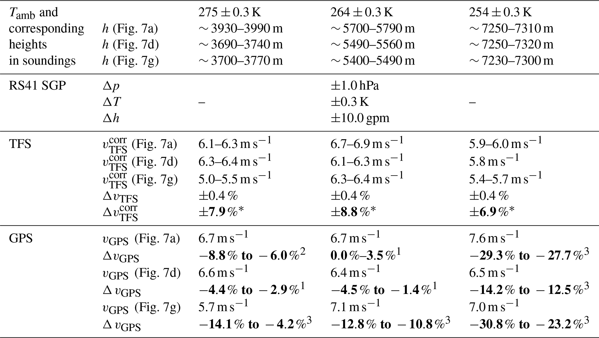
Table 5 summarises the main uncertainties arising from the different methods for determining a flow velocity through UCASS and which have equal quantitative impact on resulting particle number concentrations. From the Gaussian error propagation of the relationship given in Eqs. (1) and (2), an overall uncertainty $\mathrm{\Delta }{v}_{\mathrm{TFS}}^{\mathrm{corr}}$ combines (a) the uncertainties in T and p measured with a radiosonde RS41 SGP (Vaisala, 2024), also including uncertainties arising from the TFS calibrations conditions (in p₀ and T₀), yielding Δv_TFS, and (b) the uncertainty (i.e. determined σ) obtained from the cold-chamber test under different ambient temperature conditions (cf. Sect. S1 in the Supplement). For three chosen temperatures (i.e. 275, 264, and 254 K) from these chamber experiments, the corresponding deviations of the GPS-based flow velocities (Δv_GPS) from corresponding $v_{\mathrm{TFS}}^{\mathrm{corr}}$ are determined under equal temperature conditions during three vertical soundings (Fig. 7 and Sect. 4.1 and 4.2). Thus, the total uncertainty in $v_{\mathrm{TFS}}^{\mathrm{corr}}$ is fairly consistent within a range between 6.9 % and 8.8 % (bold values with superscript “1” in Table 5). In a few of the conditions selected here (275 and 264 K), the resulting Δv_GPS is comparatively low (values framed between two vertical lines in Table 5) or in a fairly similar range of $\mathrm{\Delta }{v}_{\mathrm{TFS}}^{\mathrm{corr}}$ values (superscript ”2”); however, in other cases (superscript ”3”), the offset in v_GPS is significant and can exceed 30 % (and occasionally even more, as seen in Fig. 7d). In essence, v_GPS appears to be the more precise measurement but can unpredictably become highly inaccurate upon vertical sounding over large height ranges (500–1500 m). In contrast, $v_{\mathrm{TFS}}^{\mathrm{corr}}$ is presumably the more accurate but less precise measurement over the discussed vertical range up to ∼ 7.5 km.

5 Summary and conclusions

This study indicates a possible improvement of the Universal Cloud and Aerosol Sounding System (UCASS), a balloon-borne optical particle counter, to obtain aerosol and cloud droplet concentration measurements with increased accuracy. The integration of a thermal flow sensor (TFS) into the UCASS allows for direct, real-time, and continuous flow velocity measurements in the immediate vicinity of UCASS's particle detection region. This approach resolves inaccuracies arising from the conventional reliance on GPS or pressure-based balloon ascent velocities, which do not account for gusts or strong wind shear, payload oscillations, flow distortions (caused by the UCASS housing), and particularly the deflection of the UCASS body from an iso-axial alignment during ascent.

Wind tunnel experiments showed that the UCASS internal flow velocity, when iso-axially aligned with the ambient airflow, is on average 11.3 % faster than the surrounding external flow (between 2–8 m s⁻¹), which is largely consistent with previous investigations. Hence, the airflow dynamics of the UCASS are reproducible and predictable under controlled conditions. Further laboratory experiments under variable angles of attack (AOAs) revealed that with a deflection of the UCASS by around 20–30°, the UCASS internal flow velocity is reduced to values approximately corresponding to the external flow velocity.

It was found that high-resolution calibrations of a TFS provide accurate results that are parameterisable according to King's law, with deviations of no more than 1.3 % from the mean samples. A more efficiently implementable three-point calibration (TPC) method (using flow velocities of approximately 2, 5, and 8 m s⁻¹) showed deviations of less than 2.9 % compared to detailed calibrations.

During balloon soundings, UCASS internal flow velocities could deviate significantly from the GPS or pressure-based ascent rates, varying by up to 30 %. Thus, accurate measurements of particle concentrations based solely on GPS or p-derived ascent rates are subject to considerable uncertainty. Vertical profiles from three soundings up to 7.5 km (see Sect. 4) showed that the deviations in flow velocity increased with increasing altitude due to changing atmospheric conditions and balloon payload geometry (i.e. the inclination of the payload orientation and thus the UCASS alignment). Referring to the thought model of the balloon sounding (see Sect. 1) – that the flight pattern of the balloon is driven by the horizontal wind components (i.e. u and v>0) – then (1) the balloon body acts as a sail with its comparatively large surface and (2) the comparatively small payload is towed. In other words, even if the main wind components with respect to the payload's inertial system (u_rel, v_rel) were nearly zero, this would typically result in a constellation of the balloon payload geometry which causes a flow towards UCASS with a non-zero AOA. While UCASS is aligned with the cord to the balloon, it is deflected with respect to the buoyancy-induced vertical lift; i.e. iso-axial flow to the UCASS is rarely given. The actual flow, which is affected by the pendulum motion and rotation of the payload and their superposition, is hardly reproducible or quantifiable. This ultimately underlines the need for a continuous measurement of the actual UCASS internal flow during the entire flight.

Hence, for airborne particle measurements, the calculated particle concentrations from UCASS detections based on GPS or pressure ascent rates may introduce errors of up to 30 %. Real-time TFS data would reduce this uncertainty by ensuring that the actual air volume of the samples is determined independently of external conditions. The integration of the TFS into the UCASS therefore represents an improvement in the methodology of measuring aerosol and cloud droplet concentrations up to 7.5 km. By providing direct and precise flow velocity measurements, the TFS avoids the limitations of GPS or p-based methods, including errors caused by payload movements, gusts, wind shear, and flow deviations caused by the shape of the UCASS housing. Field tests confirmed that this approach leads to more accurate assessments of air volumes in the samples and can reduce uncertainty in calculating particle number concentrations.

The knowledge gained may motivate future modifications and improvements in the further development of the balloon-borne UCASS instrument. The robust three-point calibration methods applied in this study facilitate the technical effort involved in integrating TFSs into a modified UCASS. This work can provide a basis for improved vertical profiling of aerosols and cloud elements with cost-effective and flexible instruments such as UCASS.