Simulations of spectral polarimetric variables measured in rain at W-band

In this work, the T-matrix approach is exploited to produce simulations of spectral polarimetric variables (spectral differential reflectivity, sZ_DR, spectral differential scattering phase, sδ_HV, and spectral correlation coefficient, sρ_HV) for observations of rain acquired from slant-looking W-band cloud radar. The spectral polarimetric variables are simulated with two different methodologies, taking into account instrument noise and the stochastic movement of the raindrops, introduced by raindrop oscillations and by turbulence. The simulated results are then compared with rain Doppler spectra observations from W-band radar for moderate rain rate conditions. Two cases, differing in levels of turbulence, are considered. While the comparison of the simulations with the measurements presents a reasonable agreement for equi-volume diameters less than 2.25 mm, large discrepancies are found in the amplitude (but not the position) of the maxima and minima of sZ_DR and, more mildly, of sδ_HV. This pinpoints a general weakness in approximating raindrop as spheroids to simulate radar backscattering properties at the W-band.

1 Introduction

Cloud radar observations are crucial for understanding cloud microphysics, as proposed in the groundwork laid by radar pioneers (Atlas et al., 1973; Lhermitte, 1990). In the last 25 years, this has been corroborated by an abundance of studies based on vertically pointing spectral Doppler cloud radar observations in multi-frequency configurations and/or in synergy with lidar and radiometers for better characterizing drizzle (e.g., O'Connor et al., 2005; Kollias et al., 2011; Luke and Kollias, 2013), rain (Kollias et al., 2001, 2002; Tridon et al., 2013; Tridon and Battaglia, 2015; Courtier et al., 2022), ice (Kalesse et al., 2016; Kneifel et al., 2016; Li et al., 2021; Luke et al., 2021), mixed-phase clouds (Luke et al., 2010), and melting particles (e.g., Li and Moisseev, 2019; Mróz et al., 2021). Polarimetric variables provide additional constraints on hydrometeor shape and orientation and are routinely measured by ground-based precipitation radar networks using low-elevation scanning strategies (Chandrasekar et al., 2023, and references therein). However, vertically pointing cloud radars miss most of the polarimetric information of hydrometeors (with the sole exception of the linear depolarization ratio; Mróz et al., 2021), since hydrometeors tend to fall with their maximum dimensions horizontally aligned. In order to overcome this limitation, more recently, a few sites started operating cloud radars with Doppler and polarimetric capabilities in slant observation mode (Myagkov et al., 2020; Unal and van den Brule, 2024; Mak and Unal, 2025). This configuration has the critical advantage that particles with different sizes are separated in the spectral domain (because they have different sedimentation velocities), which allows the contributions of different particle types to be disentangled. While vertically pointing radars can also achieve this separation, radars in slant polarization mode additionally exploit polarimetric measurements. At higher frequencies like the W-band, where multiple resonances occur across the particle size distribution (PSD), the polarimetric variables – resulting from integration over the entire PSD – tend to average out the characteristic features of single-particle scattering, often balancing positive and negative contributions (Kollias et al., 2011). This is especially evident in the simulations of differential reflectivity (Z_DR), where this parameter exhibits very low values and sensitivity to PSD variations (Unal and van den Brule, 2024). Further, the polarimetric variables reflect both scattering and propagation effects. A way to mitigate these challenges at millimeter wavelengths is to analyze polarimetric variables in the spectral domain.

For K_a- and W-band observations of rain at a 45° elevation angle, Unal and van den Brule (2024) have demonstrated that using the Rayleigh plateau, as proposed in the literature (Tridon et al., 2013; Myagkov et al., 2020), allows for the separation of propagation and backscatter contributions in the spectral domain for polarimetric variables, specifically the differential phase shift and differential reflectivity. The differential phase at backscattering can then be utilized to infer the characteristic droplet diameter of the drop size distribution (DSD). Incidentally, W-band polarimetric radar observations at slant angles have also been proposed in the framework of the ESA spaceborne WIVERN mission (Illingworth et al., 2018; Battaglia et al., 2022), which aims to measure in-cloud winds by using the polarization diversity technique with an antenna scanning conically at an incidence angle of 41.6°. Although in the WIVERN case no spectral measurements are envisaged, this mission will provide an unprecedented abundance of incidental cloud radar polarimetric observations globally.

Spectral polarimetric observations, utilizing either slant or horizontal profiling, effectively distinguish hydrometeors from clutter (Bachmann and Zrnić, 2007; Moisseev and Chandrasekar, 2009; Unal, 2009; Chen et al., 2022) and also enable the characterization of various hydrometeors (Spek et al., 2008; Pfitzenmaier et al., 2018; Wang et al., 2019; Lakshmi et al., 2024). In the case of rain, Moisseev et al. (2006) derived the shape–size relationship, while Yanovsky (2011) explored the effects of turbulence on spectral Z_DR. These studies were conducted at centimeter-wavelength frequencies.

In order to build quantitative retrieval algorithms based on spectral polarimetric observations, forward model simulators of the polarimetric spectra themselves are needed. Simulations of Doppler spectra observed by ground-based vertically pointing radar have been pioneered by Zrnić (1975) and have been applied to different hydrometeors and to millimeter radar by different authors (e.g., Kollias et al., 2011; Tridon and Battaglia, 2015; Courtier et al., 2024), including turbulence effects and raindrop inertia (Zhu et al., 2023). The simulation of polarimetric spectra (Myagkov et al., 2020; Unal and van den Brule, 2024) has been explored only marginally because slant observations are not so common.

Electromagnetic scattering properties of rain have been historically computed by assuming spheroid or Chebyshev shapes (both rotationally symmetric) via the T-matrix method (Mishchenko et al., 2000). Such models have been found satisfactory to explain radar and radiometric measurements in the S, C, X, K_u, and K_a bands (Battaglia et al., 2010; Kumjian et al., 2019; Teng et al., 2018) but they have also been used to simulate higher radar frequencies (Aydin and Lure, 1991; Kneifel et al., 2020; Unal and van den Brule, 2024). However, raindrops generally change due to oscillations, which cause departure from rotationally symmetric shapes. The T-matrix method can, in principle, simulate scattering from non-rotationally symmetric particles (given numerical convergence; Wriedt, 2002), but such implementations are computationally demanding and not widely available. As a result, most T-matrix applications rely on the assumption of rotationally symmetric particles. Different studies have highlighted the strong impact of the shape assumptions in modifying the polarimetric variables (e.g., compared sphere, spheroids, and equilibrium/Chebyshev drops; Ekelund et al., 2020), particularly when considering particles in the resonance regions (Thurai et al., 2007) (that occur in the 5.5–7 mm diameter region at the C band and at smaller sizes and in multiple ranges with increased frequency). Such studies, however, are based on a study of the DSD-integrated polarimetric variables and therefore do not fully capture the impact of the shape of each single particle. Combining Doppler and polarimetric measurements, spectral polarimetry has the potential to test hydrometeor shape models and their associated scattering properties in great detail.

Therefore, the first goal of this study is to explore how different assumptions that are related to atmospheric conditions (turbulence) and white noise of a real radar spectrum impact the simulated spectral polarimetric variables. The second objective is to present a novel comparison between simulated and observed data.

The paper is structured as follows. First we detail the methodology for simulating the cloud radar spectra and polarimetric variables (Sect. 2); then we present the results of our simulations, describe the observational dataset, compare simulations and observations, and discuss the implications of our findings.

2 Methodology for simulations

2.1 Rain scattering properties simulated by T-matrix

The simulations are generated by using a Python package to compute the electromagnetic scattering properties of non-spherical particles using the T-matrix method (Leinonen, 2014).

In this study, the rain scattering properties are exclusively targeted. The backscattering amplitude matrix, S, and the phase matrix, Z (Mishchenko et al., 2000, Chapter 16), are calculated for drops of different diameter, D, with axis ratios parameterized according to Keenan et al. (2001), Andsager et al. (1999), and Beard and Chuang (1987). The following equation is employed to describe the raindrop axis ratio:

$$\begin{array}{}\text{(1)}& \begin{array}{rl}& {\displaystyle \frac{a}{b}}\left(D\right)=\\ & \left\{\begin{array}{l}\begin{array}{rl}& \mathrm{1}/(\mathrm{0.9939}+\mathrm{0.00736}\cdot D-\mathrm{0.018485}\cdot D^{\mathrm{2}}\\ & +\mathrm{0.001456}\cdot D^{\mathrm{3}}),\end{array}\\ D<\mathrm{0.89}\mathrm{mm}\\ \begin{array}{rl}& \mathrm{1}/(\mathrm{1.0048}+\mathrm{5.7}\times {\mathrm{10}}^{-\mathrm{4}}D-\mathrm{2.628}\times {\mathrm{10}}^{-\mathrm{2}}{D}^{\mathrm{2}}\\ & +\mathrm{3.682}\times {\mathrm{10}}^{-\mathrm{3}}{D}^{\mathrm{3}}-\mathrm{1.677}\times {\mathrm{10}}^{-\mathrm{4}}{D}^{\mathrm{4}}),\end{array}\\ D\ge \mathrm{0.89}\mathrm{mm},\end{array}\right.\end{array}\end{array}$$

where $a/b$ denotes the ratio of the major to minor axes of the oblate spheroid. The use of two different formulations reflects the physical differences in raindrop deformation regimes. For small raindrops, the axis ratio follows the parameterization by Keenan et al. (2001), while for larger drops, the fit of Andsager et al. (1999) to the model of Beard and Chuang (1987) is used.

The brown line in Fig. 1 represents the axis ratio parameterization used in this study and is plotted against the equivalent relationship of Thurai et al. (2008) (dashed green line) and the axis ratio for spheres (dotted purple line). The first two lines present great agreement for particles with equi-volume diameters up to 3 mm. Very small droplets are conceived as perfect spheres (axis ratio≈1). As their size increases, drops are modeled as spheroid particles and an oblate shape is assumed (axis ratio>1). The scattering geometry of the simulation corresponds to a radar pointing at a 45° elevation angle. Raindrops are assumed to be partially aligned with their maximum dimension preferentially on the horizontal plane: scattering properties are averaged over Gaussian distributions of canting angles with different standard deviations. The raindrops are assumed to be at 10 °C; the complex relative permittivity of water at this temperature is 3.2−1.8ı at 94 GHz (Lhermitte, 1990).

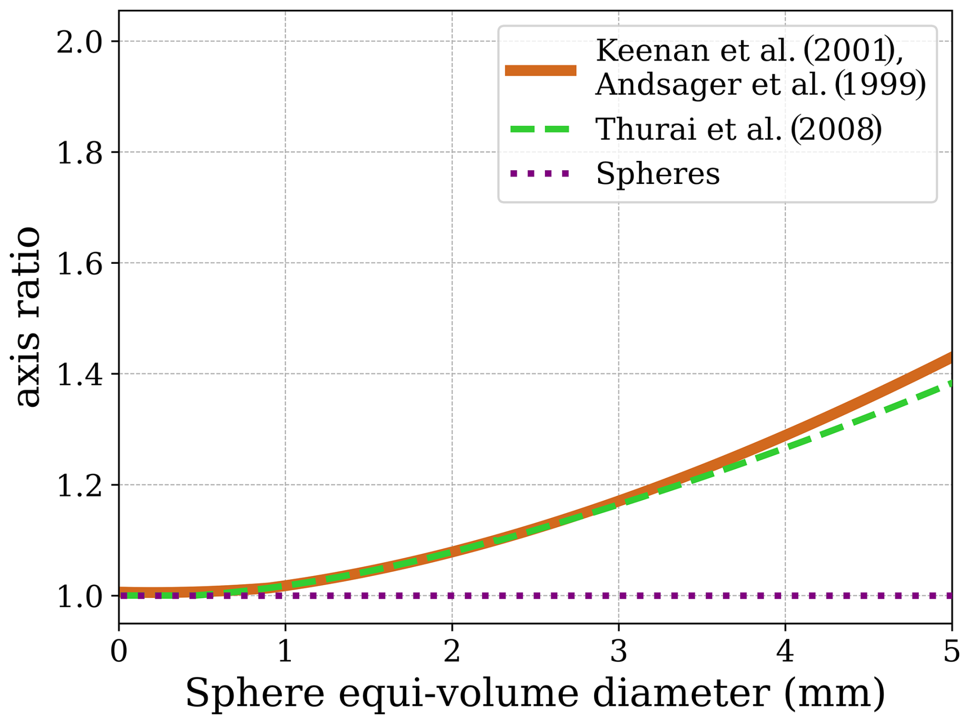
Figure 1 Axis ratio (major to minor axis) parameterization as a function of equi-volume diameters. The brown line is used in this study and is calculated according to Keenan et al. (2001) and Andsager et al. (1999). The dashed green line is the parameterization of Thurai et al. (2008) and the dotted purple line is the axis ratio of spheres.

2.1.1 Computation of single-particle polarimetric variables

The phase matrix Z describes how an electromagnetic wave is scattered by a particle and how the scattering affects its polarization state (Mishchenko et al., 2000). It is a 4×4 matrix that transforms the Stokes vector of an incident electromagnetic wave to the Stokes vector of the scattered wave. From the elements Z_ij(D) of this matrix, the following backscattering quantities can be computed.

• Backscattering cross sections for V-polarized and H-polarized radiation:

  $$\begin{array}{}\text{(2)}& \begin{array}{r}{\mathit{\sigma }}_{\mathrm{VV}}\left(D\right)=\mathrm{2}\mathit{\pi }(Z_{\mathrm{11}}+Z_{\mathrm{12}}+Z_{\mathrm{21}}+Z_{\mathrm{22}})\left[{\mathrm{mm}}^{\mathrm{2}}\right],\\ {\mathit{\sigma }}_{\mathrm{HH}}\left(D\right)=\mathrm{2}\mathit{\pi }(Z_{\mathrm{11}}-Z_{\mathrm{12}}-Z_{\mathrm{21}}+Z_{\mathrm{22}})\left[{\mathrm{mm}}^{\mathrm{2}}\right].\end{array}\end{array}$$

• Differential reflectivity:

  $$\begin{array}{}\text{(3)}& Z_{\mathrm{DR}}\left(D\right)=\mathrm{10}{\log }_{\mathrm{10}}{\displaystyle \frac{{\mathit{\sigma }}_{\mathrm{HH}}\left(D\right)}{{\mathit{\sigma }}_{\mathrm{VV}}\left(D\right)}}\left[\mathrm{dB}\right].\end{array}$$

• Copolar correlation coefficient:

  $$\begin{array}{}\text{(4)}& \begin{array}{rl}& {\mathit{\rho }}_{\mathrm{HV}}\left(D\right)=\\ & {\displaystyle \frac{\sqrt{(Z_{\mathrm{33}}+Z_{\mathrm{44}}{)}^{\mathrm{2}}+(Z_{\mathrm{43}}-Z_{\mathrm{34}}{)}^{\mathrm{2}}}}{\sqrt{(Z_{\mathrm{11}}-Z_{\mathrm{12}}-Z_{\mathrm{21}}+Z_{\mathrm{22}})(Z_{\mathrm{11}}+Z_{\mathrm{12}}+Z_{\mathrm{21}}+Z_{\mathrm{22}})}}}.\end{array}\end{array}$$

• Differential phase:

  $$\begin{array}{}\text{(5)}& {\mathit{\delta }}_{\mathrm{HV}}\left(D\right)=\arctan \left({\displaystyle \frac{Z_{\mathrm{43}}-Z_{\mathrm{34}}}{Z_{\mathrm{33}}+Z_{\mathrm{44}}}}\right)\left[\mathit{°}\right].\end{array}$$

The normalized backscattering cross section of an oblate spheroid raindrop is shown in Fig. 2 with brown color. The axis ratio for this computation is the same as the brown line of Fig. 1. The dashed green line represents the same quantity but computed by using the axis ratio parameterization of Thurai et al. (2008) (green line in Fig. 1). The same applies for the purple dotted line, which is produced by using the spheres' axis ratio. The parameterizations for the two different spheroids result in nearly identical curves, indicating that the choice of axis ratio for oblate shapes does not significantly affect the backscattering cross section behavior. In contrast, the spherical parameterization shifts the Mie notches slightly to the left, due to the different geometry of the scatterers. The positions of the first, second, and third Mie notches are indicated by the dashed blue lines at D=1.68 mm, D=2.88 mm, and D=4.13 mm, respectively.

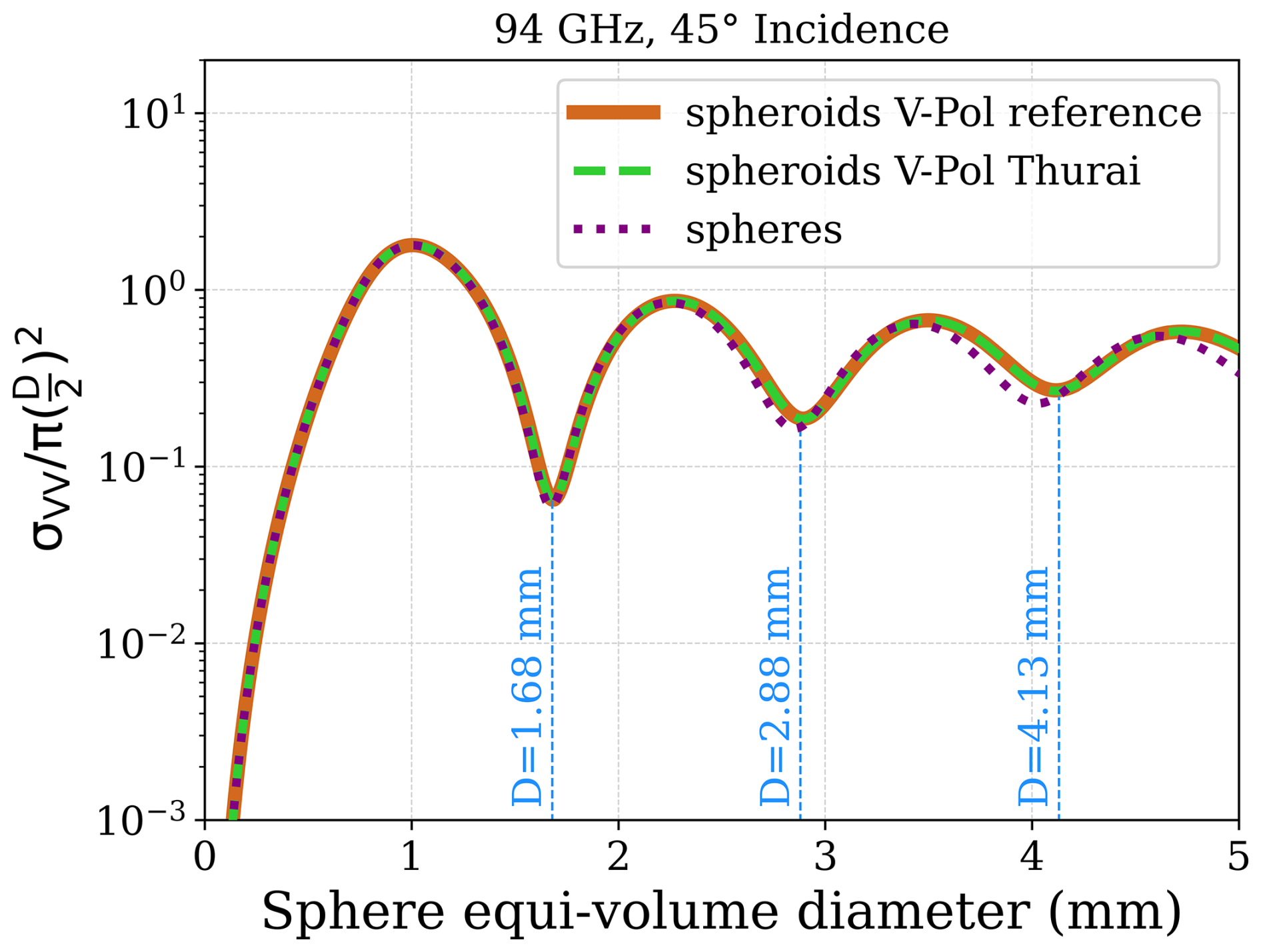
Figure 2 Normalized backscattering cross section of oblate spheroid model raindrops when pointing at 45° elevation, as a function of the sphere equi-volume diameter D. The dashed light blue lines indicate the first (D=1.68 mm), second (D=2.88 mm), and third (D=4.13 mm) Mie notches.

Some T-matrix results for the polarimetric variables are displayed in Figs. 3 and 4: different drop orientation conditions and raindrop axis ratios are considered. The dashed black lines and the blue lines are calculated by assuming perfectly oriented raindrops with axis ratio parameterization, as proposed by Thurai et al. (2008) and according to Eq. (1), respectively. In Fig. 3, those two lines are almost identical up to approximately 3 mm diameter but they diverge afterwards. Notably, for larger raindrops, the dashed black line aligns closely with the light blue line, which represents a wobbling raindrop with a 5° canting angle on average. This suggests that the same amplitudes of the maxima and minima in the spectral polarimetric variables can be achieved by different combinations of axis ratio parameterizations and varying degrees of wobbling. Therefore, in the following, the parameterization of Eq. (1) is used in combination with different degrees of wobbling.

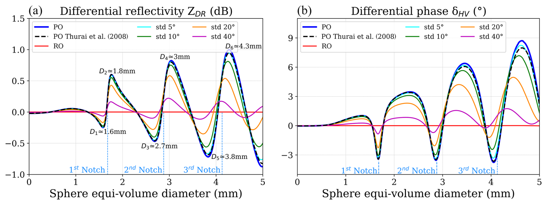
Figure 3 Simulations of (a) differential reflectivity, Z_DR, and (b) differential phase, δ_HV, as a function of sphere equi-volume diameter, for 94 GHz radar pointing at 45°. Perfect orientation (PO) and random orientation (RO) are represented by the dark blue and red lines, respectively, derived with axis ratio parameterization according to Eq. (1). The dashed black line also corresponds to perfectly oriented raindrops with axis ratio parameterization as proposed by Thurai et al. (2008). The remaining lines represent different degrees of raindrop wobbling, with a Gaussian distribution around the horizontal with standard deviations of 5° (light blue), 10° (green), 20° (orange), and 40° (pink).

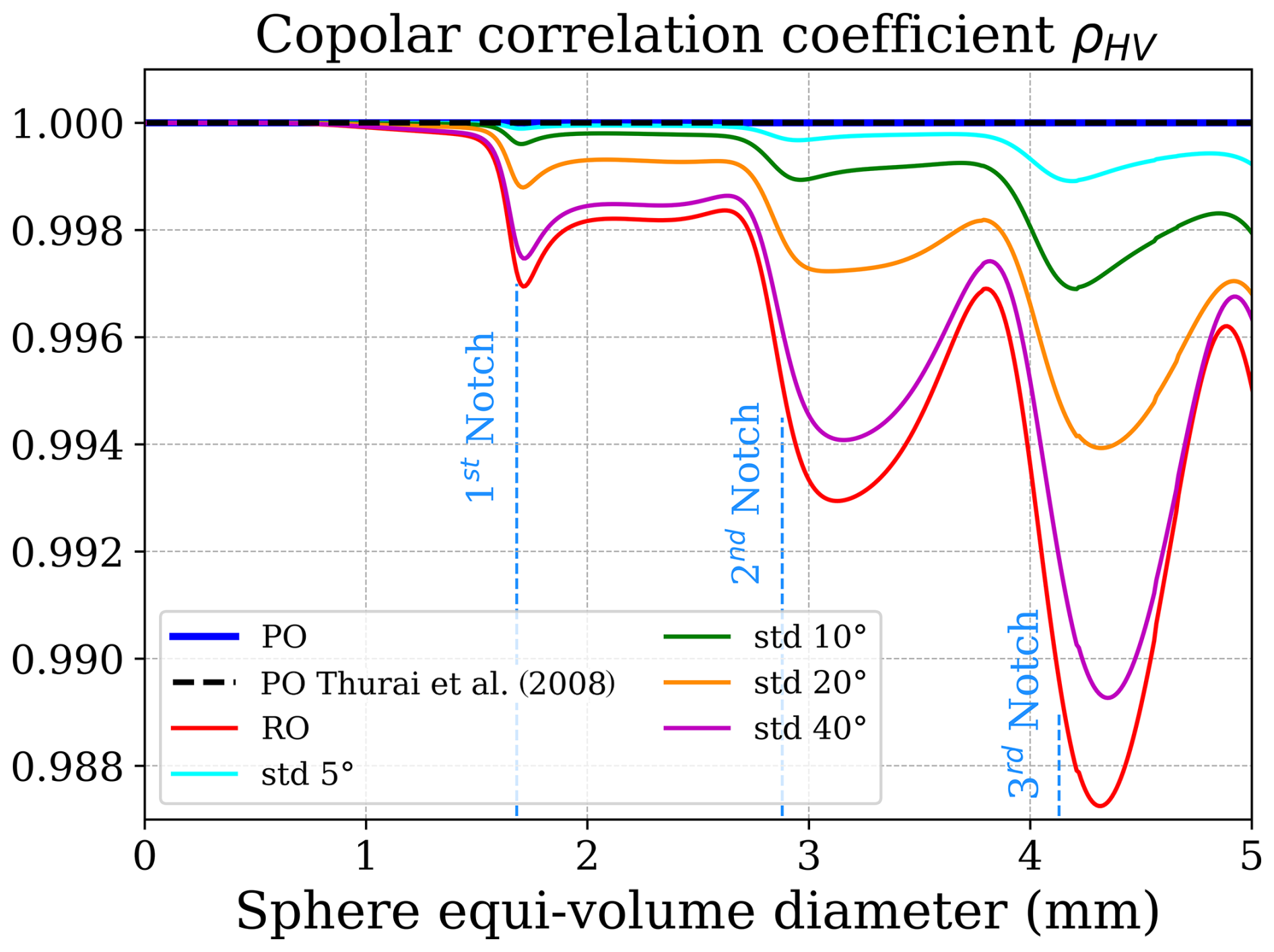
Figure 4 As Fig. 3 but for the copolar correlation coefficient, ρ_HV, as a function of sphere equi-volume diameter, for 94 GHz radar pointing at an elevation of 45°.

The differential phase (δ_HV) refers to the phase shift introduced at backscattering between the horizontally and vertically polarized components of the received radar signal. This parameter depends on the size of the hydrometeors and provides information about their shape and orientation. In Fig. 3b, δ_HV remains near 0 for small drop diameters, consistent with Rayleigh scattering. As the diameter increases, δ_HV departs from 0 and exhibits oscillatory behavior, attributed to resonance effects and the transition from spherical to oblate shapes. These fluctuations become more pronounced at larger diameters. Variability in drop orientation within the radar sampling volume, described by the canting angle distribution, further contributes to the observed variations in δ_HV. The broader the width of the canting angle distribution, the lower the magnitude of the polarimetric variables. When particles are randomly oriented (red line in Fig. 3), their orientations are distributed uniformly in all directions. In this case, the ensemble-averaged response over all possible orientations leads to cancellation effects in the differential phase (δ_HV=0, Fig. 3b) and in the differential reflectivity (Z_DR=0 dB, Fig. 3a). The cancellation occurs because, for a medium that is a mixture of randomly oriented particles, the off-diagonal elements Z₁₂, Z₂₁, Z₃₄, Z₄₃ of the phase matrix become 0 (as shown in Mishchenko et al., 2000, Chapter 3, Table II), thus leading to Z_DR=0 and δ_HV=0 (see Eqs. 3–5). The dashed blue lines of Figs. 3 and 4 indicate the positions of the Mie notches, as depicted in Fig. 2. The first two minima of δ_HV coincide with the Mie notches, while Z_DR is approximately 0 at these points. Moreover, the diameters of the minima (D₁, D₃, D₅) and maxima (D₂, D₄, D₆) are demonstrated for Z_DR.

The copolar correlation coefficient (ρ_HV) quantifies the correlation between the horizontally and vertically polarized components of the radar signal. In Fig. 4, perfectly oriented drops (solid blue and dashed black lines) have ρ_HV=1. Conversely, raindrops with variations in the orientation or tilt of the drop axis relative to the direction of motion (canting) have ρ_HV slightly lower than 1, showing a minimum loss of correlation between the two different polarization states. A broader distribution of canting angles would lead to further decorrelation. Even when considering randomly oriented raindrops, ρ_HV never falls short of 0.986. Realistic values of canting generally do not exceed 10° (Mishchenko et al., 2000). However, neither antenna pattern effects, nor antenna coupling for the quasi-bistatic radar configuration, nor multiple scattering, nor noise, was included in the calculations of ρ_HV at this stage. One, or a combination, of these effects may drive ρ_HV below 0.986.

2.1.2 Drop size distribution and raindrop velocities

The gamma distribution is a mathematical shape typically used to represent the variability of a natural rainfall drop size distribution (DSD) (Ulbrich, 1983):

$$\begin{array}{}\text{(6)}& N\left(D\right)=N_{\mathrm{0}}{D}^{\mathit{\mu }}\exp (-\mathrm{\Lambda }D)\left[{\mathrm{mm}}^{-\mathrm{1}}{\mathrm{m}}^{-\mathrm{3}}\right],\end{array}$$

where D [mm] is the sphere equi-volume diameter, μ is the dimensionless shape parameter, N₀ [${\mathrm{mm}}^{-\mathrm{1}-\mathrm{\mu }}{\mathrm{m}}^{-\mathrm{3}}$] is the number concentration parameter, and Λ [mm⁻¹] is the slope parameter. The three parameters (N₀, μ, and Λ) of the gamma distribution enable a wide range of rainfall situations to be described. The parameter Λ can be derived from Λ $=(\mathrm{4}+\mathit{\mu })/D_{\mathrm{m}}$, where D_m [mm] is the mass-weighted mean diameter (Ulbrich and Atlas, 2007; Testud et al., 2001).

Importantly for Doppler applications, the larger the drops, the faster the terminal fall speed, v_T. The relationship between the drop diameters and the corresponding velocities is parameterized  in  SI units following Frisch et al. (1995)  and Atlas et al. (1973):

$$\begin{array}{}\text{(7)}& \begin{array}{rl}& v_{\mathrm{T}}\left(D\right)=\\ & \left\{\begin{array}{l}{v}_{\mathrm{cloud}}=\mathrm{1.2}\times {\mathrm{10}}^{\mathrm{8}}\cdot {\left(\frac{D}{\mathrm{2}}\right)}^{\mathrm{2}},\\ D<\mathrm{0.11}\times {\mathrm{10}}^{-\mathrm{3}}\mathrm{m}\\ v_{\mathrm{drizzle}}=\mathrm{8333}\cdot \frac{D}{\mathrm{2}}-\mathrm{0.0833},\\ \mathrm{0.11}\times {\mathrm{10}}^{-\mathrm{3}}\le D\le \mathrm{0.86}\times {\mathrm{10}}^{-\mathrm{3}}\mathrm{m}\\ v_{\mathrm{rain}}=\mathrm{9.65}-\mathrm{10.3}\cdot {\mathrm{e}}^{-\mathrm{0.6}\times {\mathrm{10}}^{\mathrm{3}}\cdot D},\\ D>\mathrm{0.86}\times {\mathrm{10}}^{-\mathrm{3}}\mathrm{m}\end{array}\right.\end{array}.\end{array}$$

A factor of $({\mathit{\rho }}_{\mathrm{0}}/\mathit{\rho }{)}^{\mathrm{0.4}}$, with ρ₀ being the density at sea level, applies for different air densities.

In Fig. 5, raindrop terminal velocities are plotted against the diameters according to Eq. (7) and the parameterization from Thurai and Bringi (2005) (solid brown and dashed black lines, respectively). The relative difference between the two velocity parameterizations never exceeds 2 %. Therefore, when mapping terminal velocities to diameters, this translates into similar relative uncertainties in the determination of diameters for any given velocity. For instance, the position of the first (second) Mie notch is expected to occur at terminal velocities of 5.89 ± 0.11 m s⁻¹ (7.82 ± 0.15 m s⁻¹).

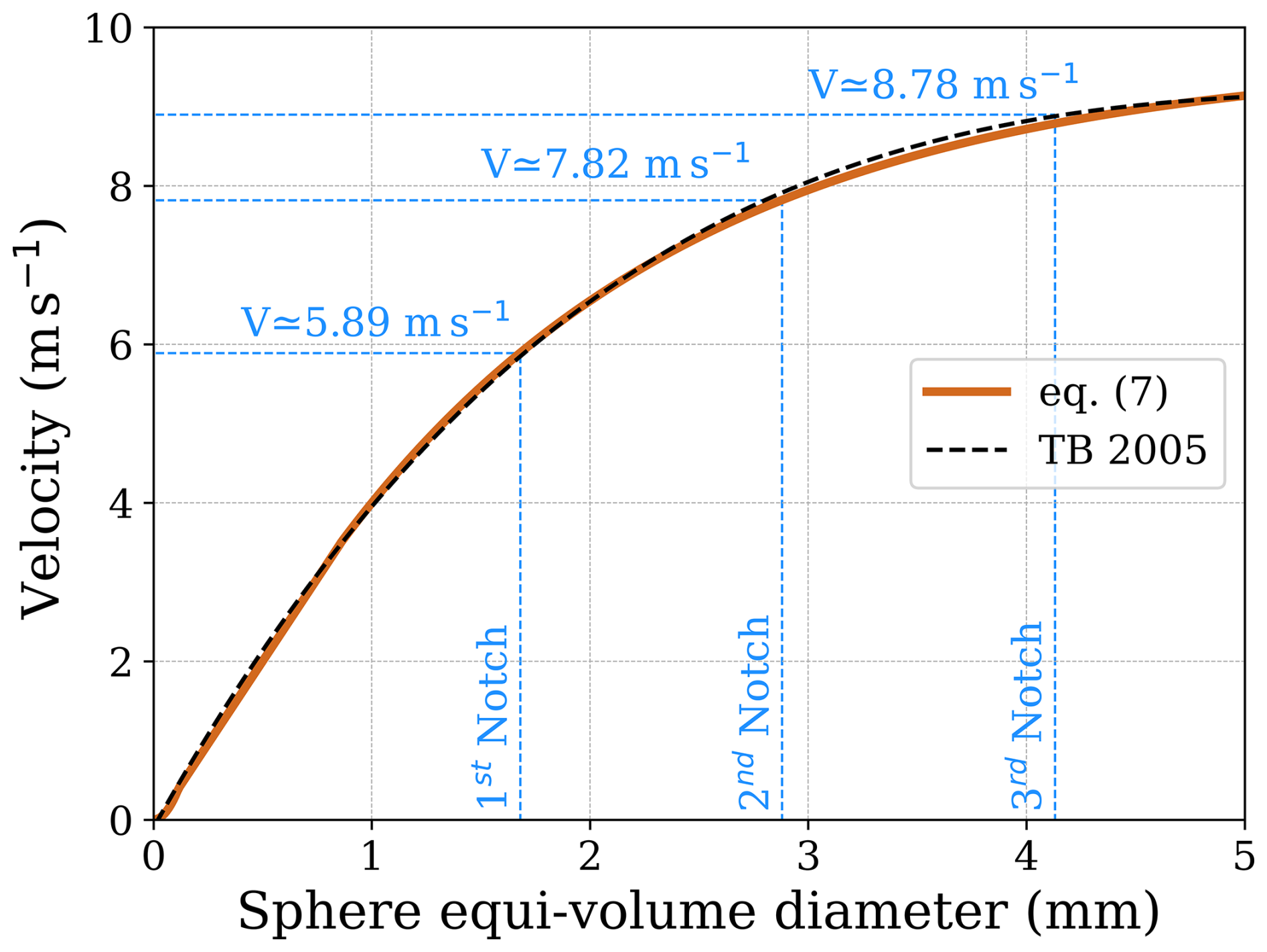
Figure 5 Terminal fall speed v_T as a function of the sphere equi-volume diameter, D, for Eq. (7), with thick brown line, and for Thurai and Bringi (2005), with dashed black line.

2.2 Simulation of spectral polarimetric variables

Two methodologies for simulating spectral polarimetric variables, as observed from W-band cloud radar, will be presented in this paper. The first was developed based on Yu et al. (2012) and Zrnić (1975), while the second is based on Thurai et al. (2008) and Chandrasekar (1986). Notably, both methods show very good agreement; they are described in detail in Sects. 2.2.1 and 2.2.2, respectively. The use of both approaches ensures that the introduced stochastic perturbations respect the physical relationships between scattering elements. Their agreement increases confidence in the simulated turbulence structure and supports the finding that observed discrepancies are not artifacts of the simulation method. Some preliminary processing is needed for both methodologies, as discussed next.

Firstly, an ideal copolar spectrum S_VV for the V channel is independently generated for each diameter (Unal, 2015):

$$\begin{array}{}\text{(8)}& S_{\mathrm{VV}}\left(v_{\mathrm{LoS}}\right)={\displaystyle \frac{{\mathit{\lambda }}^{\mathrm{4}}}{{\mathit{\pi }}^{\mathrm{5}}|K{|}^{\mathrm{2}}}}N\left(D\right){\mathit{\sigma }}_{\mathrm{VV}}\left(D\right){\displaystyle \frac{\mathrm{1}}{\sin {\mathit{\theta }}_{\mathrm{el}}}}{\displaystyle \frac{\mathrm{d}D}{\mathrm{d}{v}_{\mathrm{T}}\left(D\right)}},\end{array}$$

where λ is the radar wavelength, $\left|K^{\mathrm{2}}\right|$ is derived from the dielectric factor of water, N(D) is the DSD (see Sect. 2.1.2), σ_VV is the backscattering cross section for the V channel (Sect. 2.1.1), $v_{\mathrm{LoS}}\left(D\right)=\sin {\mathit{\theta }}_{\mathrm{el}}{v}_{\mathrm{T}}\left(D\right)+w_{\mathrm{LoS}}$ denotes the line-of-sight (LoS) Doppler velocities of the drops at the given elevation angle θ_el, and v_LoS is the sum of the components of the raindrop terminal velocity and of the wind speed along the LoS. Equation (8) is formulated for elevation angles θ_el significantly greater than 0, without accounting for the contribution of turbulence. The spectrum is mapped to the velocity domain via Eq. (7) and sampled in correspondence with the velocity points v_j, with $j=\mathrm{1},\mathrm{2},\mathrm{\dots },N_{\mathrm{FFT}}$, where N_FFT is the number of FFT points, as dictated by the Doppler velocity resolution and Nyquist interval envisaged for any given radar system. The samples are indicated as S_VV(v_j). Similarly, the H channel spectrum can also be produced at each velocity bin by replacing σ_VV(D) with σ_HH(D) in Eq. (8).

The cross spectrum, denoted S_HV(D), is derived as

$$\begin{array}{}\text{(9)}& \begin{array}{rl}{S}_{\mathrm{HV}}\left(v_{\mathrm{LoS}}\right)& ={\displaystyle \frac{{\mathit{\lambda }}^{\mathrm{4}}}{{\mathit{\pi }}^{\mathrm{5}}|K{|}^{\mathrm{2}}}}N\left(D\right)\sqrt{{\mathit{\sigma }}_{\mathrm{VV}}\left(D\right){\mathit{\sigma }}_{\mathrm{HH}}\left(D\right)}\\ & \times {\displaystyle \frac{\mathrm{1}}{\sin {\mathit{\theta }}_{\mathrm{el}}}}{\displaystyle \frac{\mathrm{d}D}{\mathrm{d}{v}_{\mathrm{T}}\left(D\right)}}{\mathit{\rho }}_{\mathrm{HV}}\left(D\right){\mathrm{e}}^{\mathit{ı}{\mathit{\delta }}_{\mathrm{HV}}\left(D\right)},\end{array}\end{array}$$

where $\mathit{ı}=\sqrt{-\mathrm{1}}$, ρ_HV(D) is the correlation coefficient between the V and H channels, and δ_HV(D) is the phase difference between the V and H channel signals, as described in Eqs. (4) and (5). The spectrum is sampled similarly to the V channel spectrum at velocity points v_j with $j=\mathrm{1},\mathrm{2},\mathrm{\dots },N_{\mathrm{FFT}}$, and the samples are denoted S_HV(v_j). Note that each Doppler velocity spectrum can be converted to the frequency domain by using the relationship $f_{\mathrm{D}}=\mathrm{2}{v}_{\mathrm{LoS}}/\mathit{\lambda }$ between frequency Doppler shift, f_D, and v_LoS.

Generally, spectra are derived at any given range from the FFT of the time series of radar sampled voltage signals, the so-called I (in-phase) and Q (quadrature) signals collected at the same range distance (Doviak and Zrnić, 1993). In the following, complex voltages will be identified with calligraphic style letters (e.g., 𝒱, 𝒩). Also, such voltages will always be expressed in the velocity domain, as indicated by their functional argument. They correspond to the FFT of the voltages expressed in the time domain.

2.2.1 Methodology I: direct computation of I and Q in the frequency domain

This method allows Doppler spectra to be simulated by working only in the velocity (frequency) domain. Following Yu et al. (2012), the time series of complex voltage signals in the V channel in the velocity domain can be written as

$$\begin{array}{}\text{(10)}& \begin{array}{l}{\mathcal{V}}_{\mathrm{V}}^{\left[\mathrm{1}\right]}(v_j,k)=\sqrt{-S_{\mathrm{VV}}\left(v_j\right)\ln u_{jk}^{\left[\mathrm{1}\right]}}{\mathrm{e}}^{\mathit{ı}{\mathit{\theta }}_{jk}^{\left[\mathrm{1}\right]}},\\ \\ j=\mathrm{1},\mathrm{2},\mathrm{\dots },N_{\text{FFT}};k=\mathrm{1},\mathrm{2},\mathrm{\dots },K,\end{array}\end{array}$$

where u^[1] and θ^[1] are independent, identically distributed, random variables with uniform distribution between 0 and 1 and between −π and π, respectively. This process can be repeated $k=\mathrm{1},\mathrm{2},\mathrm{\dots },K$ times, in order to generate K independent stochastic realizations of the same spectrum. Similarly, for the H channel in the velocity domain:

$$\begin{array}{}\text{(11)}& \begin{array}{l}\begin{array}{rl}{\mathcal{V}}_{\mathrm{H}}(v_j,k)& =\sqrt{s{Z}_{\mathrm{DR}}\left(v_j\right)}\left[s{\mathit{\rho }}_{\mathrm{HV}}\right(v_j\left){\mathcal{V}}_{\mathrm{V}}^{\left[\mathrm{1}\right]}\right(v_j,k)\\ & +\sqrt{\mathrm{1}-s{{\mathit{\rho }}_{\mathrm{HV}}}^{\mathrm{2}}\left(v_j\right)}{\mathcal{V}}_{\mathrm{V}}^{\left[\mathrm{2}\right]}(v_j,k)]{\mathrm{e}}^{\mathit{ı}s{\mathit{\delta }}_{\mathrm{HV}}\left(v_j\right)},\end{array}\\ j=\mathrm{1},\mathrm{2},\mathrm{\dots },N_{\text{FFT}},k=\mathrm{1},\mathrm{2},\mathrm{\dots },K,\end{array}\end{array}$$

where the spectral variables sρ_HV, sδ_HV, and sZ_DR are generated as described in Sect. 2.1 for each velocity bin j, but also hold the prefix s in the notation to differentiate them from the commonly used integral polarimetric variables. The series ${\mathcal{V}}_{\mathrm{V}}^{\left[\mathrm{2}\right]}(v_j,k)$ is generated according to Eq. (10), with the same model spectrum S_VV(v) but with a second independent sequence of random numbers (u^[2] and θ^[2]). This process is repeated for each velocity bin for a total of N_FFT spectral points within the Nyquist interval. The inverse Fourier transforms of 𝒱_V(v_j) and 𝒱_H(v_j), with $j=\mathrm{1},\mathrm{2},\mathrm{\dots },N_{\text{FFT}}$, represent simulated time series of complex signals for the V and H channels. For the implementation of white noise, an approach similar to Eq. (10) is used:

$$\begin{array}{}\text{(12)}& \begin{array}{l}\begin{array}{rl}{\mathcal{N}}_{\mathrm{V}}(v_j,k)& =\sqrt{-N_{\mathrm{V}}\ln u_{jk}^{\left[\mathrm{3}\right]}}{\mathrm{e}}^{\mathit{ı}{\mathit{\theta }}_{jk}^{\left[\mathrm{3}\right]}},\\ {\mathcal{N}}_{\mathrm{H}}(v_j,k)& =\sqrt{-N_{\mathrm{H}}\ln u_{jk}^{\left[\mathrm{4}\right]}}{\mathrm{e}}^{\mathit{ı}{\mathit{\theta }}_{jk}^{\left[\mathrm{4}\right]}},\end{array}\\ \\ j=\mathrm{1},\mathrm{2},\mathrm{\dots },N_{\text{FFT}},k=\mathrm{1},\mathrm{2},\mathrm{\dots },K,\end{array}\end{array}$$

where N_V and N_H are the noise power levels for the V and H channels corresponding to the prescribed values of signal-to-noise ratio (SNR), and u^[3], θ^[3], u^[4], and θ^[4] are again generated independently.

The complex numbers that represent the simulation of the noisy I and Q in the frequency domain for the V and H channels are calculated from

$$\begin{array}{}\text{(13)}& \begin{array}{l}\begin{array}{rl}{\mathcal{S}}_{\mathrm{V}}(v_j,k)& ={\mathcal{V}}_{\mathrm{V}}(v_j,k)+{\mathcal{N}}_{\mathrm{V}}(v_j,k),\\ {\mathcal{S}}_{\mathrm{H}}(v_j,k)& ={\mathcal{V}}_{\mathrm{H}}(v_j,k)+{\mathcal{N}}_{\mathrm{H}}(v_j,k),\end{array}\\ \\ j=\mathrm{1},\mathrm{2},\mathrm{\dots },N_{\text{FFT}},k=\mathrm{1},\mathrm{2},\mathrm{\dots },K.\end{array}\end{array}$$

2.2.2 Methodology II: correlation matrix

Alternatively, the I and Q generation can be performed using the methodology proposed by Unal and Moisseev (2004), based on the correlation matrix. First, the correlation matrix R is built with the Doppler power spectra in the diagonal terms and the cross-polar spectrum in the antidiagonal elements, as

$$\begin{array}{}\text{(14)}& \begin{array}{l}R\left(v_j\right)=\left(\begin{array}{cc}{S}_{\mathrm{VV}}\left(v_j\right)+N_{\mathrm{V}}& S_{\mathrm{HV}}\left(v_j\right)\\ S_{\mathrm{HV}}^{\star }\left(v_j\right)& S_{\mathrm{HH}}\left(v_j\right)+N_{\mathrm{H}}\end{array}\right),\\ \\ j=\mathrm{1},\mathrm{2},\mathrm{\dots },N_{\mathrm{FFT}},\end{array}\end{array}$$

with all terms given by Eqs. (8) and (9). Noise has also been included but with no copolar correlation. Because R is Hermitian and positive definite, it may be written as $R=T^{†}T$ via Cholesky decomposition, where ^† denotes the Hermitian transpose. Given 2N_FFT zero-mean independent standard circular Gaussian random variables, y₁, y₂, …, $y_{\mathrm{2}{N}_{\mathrm{FFT}}}$ (i.e., $y_j=\mathrm{1}/\sqrt{\mathrm{2}}({\mathit{\xi }}_j+\mathit{ı}{\mathit{\eta }}_j)$, where ξ_j and η_j are normally distributed with mean equal to 0 and standard deviation equal to 1), the complex numbers

$$\begin{array}{}\text{(15)}& \left[\begin{array}{c}{\mathcal{S}}_{\mathrm{V}}\left(v_{\mathrm{1}}\right)\\ {\mathcal{S}}_{\mathrm{H}}\left(v_{\mathrm{1}}\right)\\ {\mathcal{S}}_{\mathrm{V}}\left(v_{\mathrm{2}}\right)\\ {\mathcal{S}}_{\mathrm{H}}\left(v_{\mathrm{2}}\right)\\ \mathrm{⋮}\\ {\mathcal{S}}_{\mathrm{V}}\left(v_{\mathrm{FFT}}\right)\\ {\mathcal{S}}_{\mathrm{H}}\left(v_{\mathrm{FFT}}\right)\end{array}\right]=T^{†}\left[\begin{array}{c}{y}_{\mathrm{1}}\\ y_{\mathrm{2}}\\ y_{\mathrm{3}}\\ y_{\mathrm{4}}\\ \mathrm{⋮}\\ y_{\mathrm{2}{N}_{\mathrm{FFT}}-\mathrm{1}}\\ y_{\mathrm{2}{N}_{\mathrm{FFT}}}\end{array}\right]\end{array}$$

have components distributed as normally distributed variables with zero mean and with correlation provided by R. The procedure can be repeated K times to simulate K different spectra.

2.2.3 Computation of polarimetric variables from I and Q

Once I and Q have been obtained with either of the two methodologies, then noisy Doppler spectra can be computed as a spectral average of K spectra:

$$\begin{array}{}\text{(16)}& {\displaystyle }{S}_{\mathrm{VV}}\left(v_j\right)& {\displaystyle }=\langle \left|{\mathcal{S}}_{\mathrm{V}}\right(v_j){|}^{\mathrm{2}}\rangle ={\displaystyle \frac{\mathrm{1}}{K}}\sum _{k=\mathrm{1}}^K{\left|{\mathcal{S}}_{\mathrm{V}}(v_j,k)\right|}^{\mathrm{2}},\text{(17)}& {\displaystyle }{S}_{\mathrm{HH}}\left(v_j\right)& {\displaystyle }=\langle \left|{\mathcal{S}}_{\mathrm{H}}\right(v_j){|}^{\mathrm{2}}\rangle ={\displaystyle \frac{\mathrm{1}}{K}}\sum _{k=\mathrm{1}}^K{\left|{\mathcal{S}}_{\mathrm{H}}(v_j,k)\right|}^{\mathrm{2}}.\end{array}$$

The spectral polarimetric variables sρ_HV(v) and sδ_HV(v) are calculated according to Mishchenko et al. (2000):

$$\begin{array}{}\text{(18)}& s{\mathit{\rho }}_{\mathrm{HV}}\left(v_j\right){\mathrm{e}}^{\mathit{ı}s{\mathit{\delta }}_{\mathrm{HV}}\left(v_j\right)}={\displaystyle \frac{\langle {\mathcal{S}}_{\mathrm{H}}\left(v_j\right){\mathcal{S}}_{\mathrm{V}}^{\star }\left(v_j\right)\rangle }{\sqrt{\langle \left|{\mathcal{S}}_{\mathrm{H}}\right(v_j){|}^{\mathrm{2}}\rangle \langle |{\mathcal{S}}_{\mathrm{V}}\left(v_j\right){|}^{\mathrm{2}}\rangle }}},\end{array}$$

where $\langle {\mathcal{S}}_{\mathrm{H}}\left(v_j\right){\mathcal{S}}_{\mathrm{V}}^{\star }\left(v_j\right)\rangle$ is the average,

$${\displaystyle \frac{\mathrm{1}}{K}}\sum _{k=\mathrm{1}}^K{\mathcal{S}}_{\mathrm{H}}(v_j,k){\mathcal{S}}_{\mathrm{V}}^{\star }(v_j,k).$$

2.2.4 Inclusion of turbulence in the simulations

Understanding the effects of turbulence on the Doppler spectrum is crucial for improving the accuracy of radar observations and their interpretation. Atmospheric turbulence causes random fluctuations in the velocity of hydrometeors, thus broadening the Doppler spectrum. All droplets are here assumed to have no inertial effects and therefore act like perfect tracers. Thus, to introduce the turbulent motions of drops in the simulations, the Doppler spectra must be convolved with a turbulence term S_air:

$$\begin{array}{}\text{(19)}& \begin{array}{rl}{S}_{\mathrm{VV}}^{\text{turb}}\left(v_{\mathrm{LoS}}\right)& =(S_{\mathrm{VV}}*S_{\text{air}})\left(v_{\mathrm{LoS}}\right)\\ & =\underset{-\mathrm{\infty }}{\overset{\mathrm{\infty }}{\int }}{S}_{\mathrm{VV}}(v_{\mathrm{LoS}}-\mathit{\xi })S_{\text{air}}\left(\mathit{\xi }\right)\mathrm{d}\mathit{\xi },\end{array}\end{array}$$

where the symbol * denotes convolution, ξ is the convolution variable, and S_air accounts for the turbulent motions within the atmosphere:

$$\begin{array}{}\text{(20)}& S_{\mathrm{air}}\left(v\right)={\displaystyle \frac{\mathrm{1}}{\sqrt{\mathrm{2}\mathit{\pi }}{\mathit{\sigma }}_{\mathrm{t}}}}{\mathrm{e}}^{-\frac{v^{\mathrm{2}}}{\mathrm{2}{\mathit{\sigma }}_{\mathrm{t}}^{\mathrm{2}}}},\end{array}$$

with σ_t expressing the turbulence broadening of the Doppler spectrum. Equations similar to Eq. (19) can be used to compute the turbulence-broadened spectra $S_{\mathrm{HH}}^{\text{turb}}\left(v\right)$ for H-polarized radiation, as well as for $S_{\mathrm{HV}}^{\text{turb}}\left(v\right)$. Then the broadened $s{Z}_{\mathrm{DR}}^{\text{turb}}\left(v\right)$ can be computed as the ratio of $S_{\mathrm{HH}}^{\text{turb}}\left(v\right)$ to $S_{\mathrm{VV}}^{\text{turb}}\left(v\right)$, whereas the turbulent-broadened parameters $s{\mathit{\rho }}_{\mathrm{HV}}^{\text{turb}}$ and $s{\mathit{\delta }}_{\mathrm{HV}}^{\text{turb}}$ are then calculated as, respectively, the amplitude and the phase of the variable:

$$\begin{array}{}\text{(21)}& s{\mathit{\rho }}_{\mathrm{HV}}^{\text{turb}}\left(v\right){\mathrm{e}}^{\mathit{ı}s{\mathit{\delta }}_{\mathrm{HV}}^{\text{turb}}\left(v\right)}={\displaystyle \frac{S_{\mathrm{HV}}^{\text{turb}}\left(v\right)}{\sqrt{S_{\mathrm{HH}}^{\text{turb}}\left(v\right)S_{\mathrm{VV}}^{\text{turb}}\left(v\right)}}}.\end{array}$$

For the generation of I and Q:

• For methodology 1 (Sect. 2.2.1), the simulated spectral polarimetric variables $s{Z}_{\mathrm{DR}}^{\text{turb}}\left(v\right)$, $s{\mathit{\delta }}_{\mathrm{HV}}^{\text{turb}}\left(v\right)$, and $s{\mathit{\rho }}_{\mathrm{HV}}^{\text{turb}}\left(v\right)$ will replace the ideal quantities in Eq. (11).

• For methodology 2 (Sect. 2.2.2), $S_{\mathrm{VV}}^{\text{turb}}$, $S_{\mathrm{HH}}^{\text{turb}}$, and $S_{\mathrm{HV}}^{\text{turb}}$ are used directly in the definition of the correlation matrix in Eq. (14).

2.2.5 Rationale for simulation based on $I/Q$

The reason we chose to generate noisy spectra using $I/Q$ components, instead of working with average spectra with added noise power, is to explicitly investigate whether the use of random individual noisy spectra can help explain or reproduce the variability and degradation often observed in measured spectral polarimetric variables, particularly in variables that rely on cross-channel correlations, like S_HV, at low SNR and low correlations where approximated formulas, as demonstrated in Myagkov and Ori (2022), tend to fail.

By simulating the noisy spectra from $I/Q$ components, we aimed to test whether noise characteristics contribute to the spectral variability seen in observations. In this sense, our work seeks to fill a gap in the literature and offer an alternative angle to understanding the role of noise in radar polarimetry.

3 Comparisons with measurements

To assess the accuracy of the cloud radar simulation methods, we compare the measurements and the simulated data. This comparison aims to validate the performance of the simulations and identify any discrepancies that may arise from model assumptions or parameter settings. The cloud radar measurements were obtained using an RPG frequency-modulated continuous wave (FMCW) dual polarization W-band cloud Doppler radar system, operating at 94 GHz in a simultaneous transmission–simultaneous reception (STSR) mode. The radar system was configured to investigate polarimetric and spectral polarimetric measurements of clouds and precipitation in the troposphere for a period of 4 months (January–April 2021). The models described in Sects. 2.2.1 and 2.2.2 were initialized based on the characteristics (SNR; pulse repetition frequency, PRF; FFT bins) of the real measurements to generate simulated radar data, for comparison with the real data.

Two case studies from 3 February 2021 are presented, both characterized by moderate rainfall, with rain rates approximately between 6 and 7 mm h⁻¹. The first one focuses on a spectrum acquired at an altitude of 105 m above ground level, while the second one targets a spectrum at 484 m. The cases differ primarily in the level of atmospheric turbulence observed at specific heights. Excluding cases of strong wind shear (e.g., jet streams) and deep convective systems (e.g., thunderstorms), higher altitudes are generally characterized by significantly less turbulence than lower levels, as turbulence is mostly generated by surface heating and friction. The measured spectrogram on the vertical channel, S_V, and the polarimetric variables, sZ_DR, sδ_HV, and sρ_HV, are presented in Fig. 6. The x axis represents the Doppler velocity, v_LoS, corresponding to the unfolded measured Doppler velocity. The spectral signatures associated with small raindrops appear on the left side of the spectra. As raindrop sizes increase and become comparable to the radar wavelength, non-Rayleigh scattering occurs, leading to resonance features, observed on the right side of the spectra.

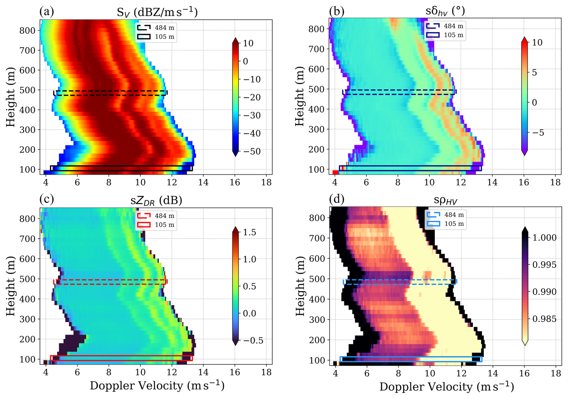
Figure 6 Event of 3 February 2021, 12:40 UTC, with vertical profiles for (a) reflectivity, (b) differential phase shift, (c) differential reflectivity, and (d) correlation coefficient spectra. The two levels that are used for case studies are marked by the solid (105 m) and dashed (484 m) rectangles.

To facilitate the comparison between simulations and observational data, the terminal velocity, v_T, was selected for the velocity axis in Sects. 3.1 and 3.2. Accordingly, the Doppler velocities shown in Fig. 6 were first adjusted along the velocity axis to remove the contribution of the radial wind, w_LoS. This correction was achieved by identifying the first Mie scattering minimum (Kollias et al., 2002). At an elevation angle of θ_el=45°, the first Mie minimum corresponds to a velocity of 5.89sin θ_el=4.16 m s⁻¹. The resulting corrected Doppler velocities, v_LoS−w_LoS, were then divided by sin θ_el, yielding an estimate of the terminal velocities for the observations.

A comparison between measured and simulated sρ_HV is challenging. The measurement of sρ_HV is subjected to biases (particularly at low signal-to-noise levels, Touzi et al., 1999) and is affected by radar-specific characteristics (e.g., antenna-related), which are difficult to quantify and account for (Myagkov et al., 2025). Therefore sρ_HV is not further analyzed in this paper.

3.1 Case study 1: moderate turbulence conditions

The Doppler spectrum measured at a height of 105 m is presented in Fig. 7 with a black line. The presence of turbulence is depicted as the broadening effect of the spectrum and the notches are smoothed out. To accurately match the measured radar spectrum, a variety of gamma drop size distributions (DSDs) were produced by adjusting the parameters described in Sect. 2.1.2, aiming to find the DSD that best fits the observed spectrum (blue line). Different combinations of μ, N₀, D_m (from Eq. 6), and σ_t (from Eq. 20) are tested to better represent the real measurement. To identify the optimal fit, the least squares method was employed. This method minimizes the sum of the squared differences between the measured and simulated spectra, ensuring that the best-fitting gamma DSD is selected. The spectra are compared in logarithmic scale rather than in linear units to better capture the wide dynamic range of radar reflectivity. In this way, both high and low reflectivity values are appropriately weighted, avoiding the dominance by large values that occurs in linear comparisons. In order to avoid overfitting the tails of the spectrum (and deteriorating the fits of the high SNR part of the spectrum, e.g., in correspondence to the Mie notch), only the part of the spectrum above the dashed purple line at −8 $\mathrm{dBZ}(\mathrm{m}{\mathrm{s}}^{-\mathrm{1}}{)}^{-\mathrm{1}}$ is fitted. That emphasizes the resonance notches – whether sharp or smoothed – providing a more robust indication of the magnitude of σ_t. This threshold is an empirical rule of thumb derived from this study, which primarily focused on cases with rain rates of 5–9 mm h⁻¹.

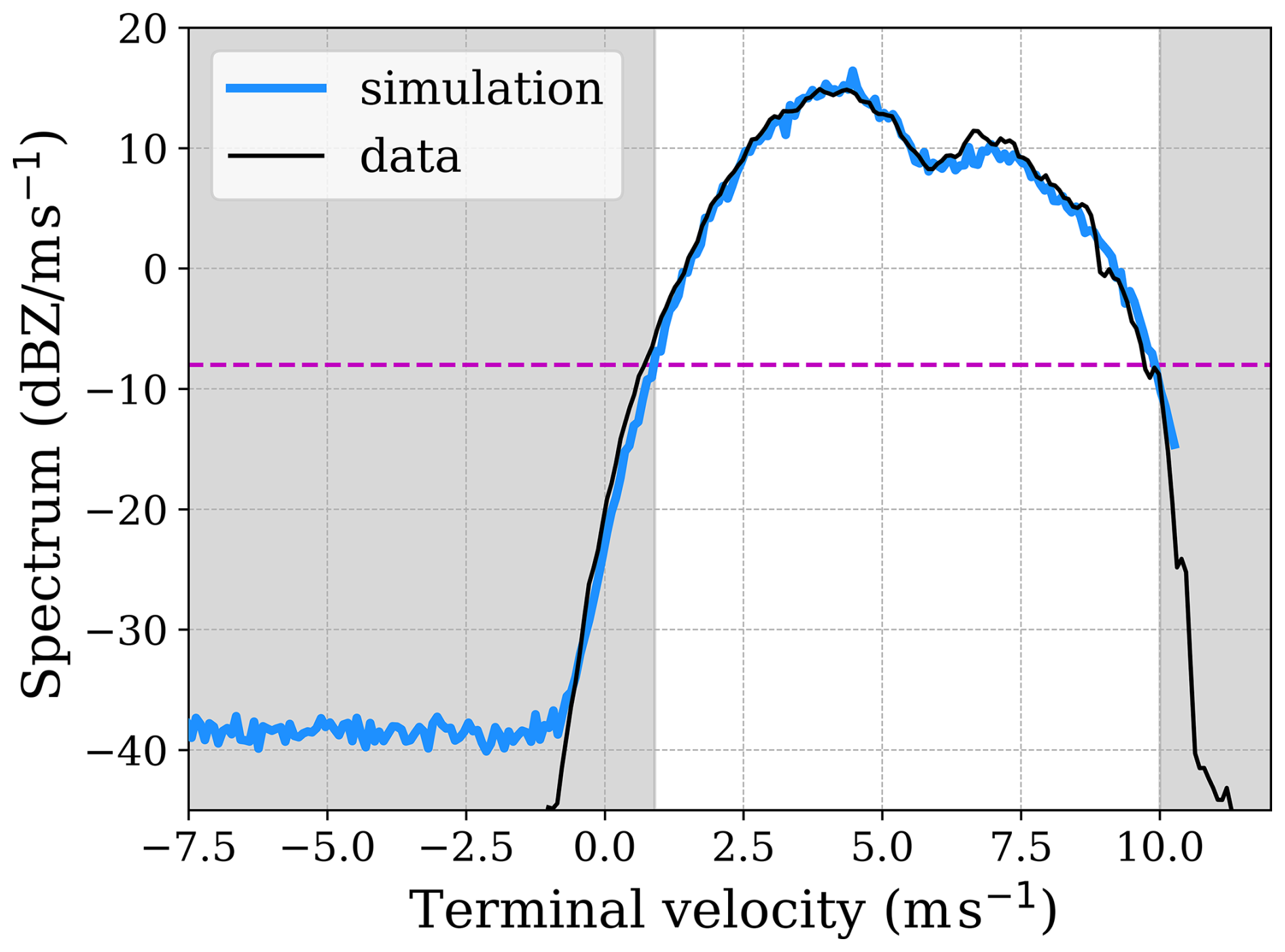
Figure 7 3 February 2021, 12:40 UTC, 105 m: measured Doppler spectrum (black line) and optimum-fitted gamma DSD (blue line). The dashed purple line indicates the threshold for applying the least squares method in order to find the optimum fit. The parameters that characterize the fitted spectrum are μ=0, D_m=1.8 mm, N₀=987 ${\mathrm{mm}}^{-\mathrm{1}-\mathrm{\mu }}{\mathrm{m}}^{-\mathrm{3}}$, and σ_t=0.5 m s⁻¹.

In Fig. 8, the black lines represent the measured spectral polarimetric variables sZ_DR (left) and sδ_HV (right), while the blue and red lines are the results of the two simulation methods, obtained by using the aforementioned optimum-fitted Doppler spectrum (see Fig. 7). Next to the radar elevation angle, the primary physical factors influencing the spectral polarimetric variables are the axis ratio–diameter relationship and the canting angle distribution (Unal and van den Brule, 2024), as well as the variability in air motion, characterized by σ_t. The values of sZ_DR and sδ_HV do not depend on the raindrop size distribution (Unal and van den Brule, 2024). However, what may vary in Fig. 8 is the terminal velocity range – for example, under low turbulence conditions, the velocity range narrows when D_m is small, as in the case of light rain.

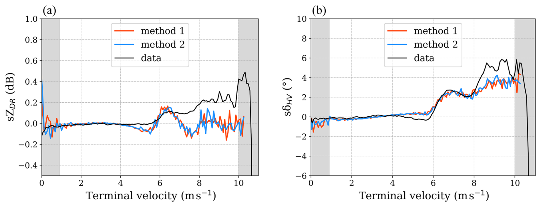
Figure 8 Spectral polarimetric variables of case study 1: (a) spectral differential reflectivity sZ_DR; (b) spectral differential phase sδ_HV. Black lines represent the measured data; blue and red lines represent the simulations from method 1 and method 2, respectively.

In order to provide a consistent reference for spherical raindrops, the measured sZ_DR and sδ_HV were adjusted along the y axis to 0 dB and 0°, respectively. The adjustment was determined based on the measured values for the smallest particles, which are expected to be nearly spherical. This correction accounts for propagation effects and instrument miscalibrations of the polarimetric variables. The spectral polarimetric variables are analyzed outside the gray-shaded regions, where the Doppler spectral power exceeds −8 $\mathrm{dBZ}(\mathrm{m}{\mathrm{s}}^{-\mathrm{1}}{)}^{-\mathrm{1}}$, to ensure a sufficiently high signal-to-noise ratio.

As expected, there is excellent agreement (within the stochastic noisiness) between the two methods used for generating the simulations (blue and red lines) for the two variables. The use of both methods described in Sect. 2.2 is to ensure that the stochastic perturbations respect the physical relationships between the scattering elements. The fact that both methods demonstrate consistency when producing the polarimetric variables provides confidence in the turbulence generation in the simulations. Conversely, while the comparison between cloud radar simulations and measurements exhibits some agreement, there are notable discrepancies that indicate limitations in the current simulation models. The primary issue is not the position of the maxima and minima, but rather the amplitude of the signal (e.g., no negative sZ_DR is observed). Although the position of the extrema may be slightly influenced by uncertainties in mapping diameters to velocity space (see Sect. 2.1.2), the key factor affecting their position is the scattering process itself. For drops with terminal velocities up to 7 m s⁻¹, the simulations and the observations of sZ_DR and sδ_HV show reasonable agreement, although, around velocities of 5 m s⁻¹, smaller values of sZ_DR and bigger values of sδ_HV are simulated, relative to the observations. However, for drops with higher terminal velocities (v_T>7 m s⁻¹), the agreement between observations and simulated data is poor, especially for the differential reflectivity. Note that these results are obtained with perfectly oriented raindrops. When increasing the canting, the amplitudes of both sZ_DR and sδ_HV are reduced and a worse correlation is obtained.

3.2 Case study 2: light turbulence conditions

In this case, the notches of the Doppler spectrum are more pronounced (Fig. 9). The best-fitting gamma DSD is represented by the blue line.

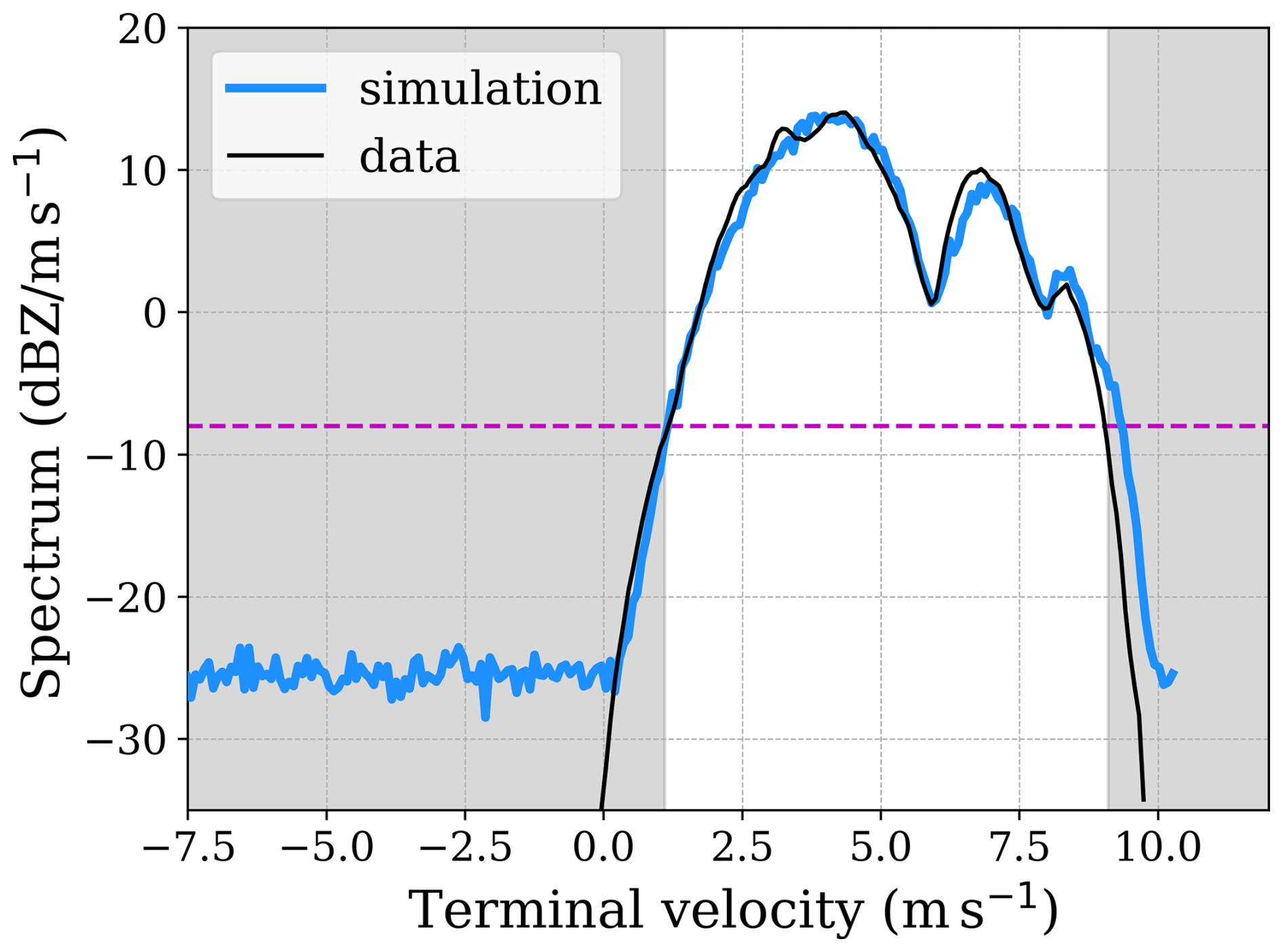
Figure 9 3 February 2021, 12:40 UTC, 484 m: measured Doppler spectrum (black line) and optimum-fitted gamma DSD (blue line). The dashed purple line indicates the threshold for applying the least squares method in order to find the optimum fit. The parameters that characterize the fitted spectrum are $\mathit{\mu }=-\mathrm{0.4}$, D_m=1.6 mm, N₀=688 ${\mathrm{mm}}^{-\mathrm{1}-\mathrm{\mu }}{\mathrm{m}}^{-\mathrm{3}}$, and σ_t=0.15 m s⁻¹.

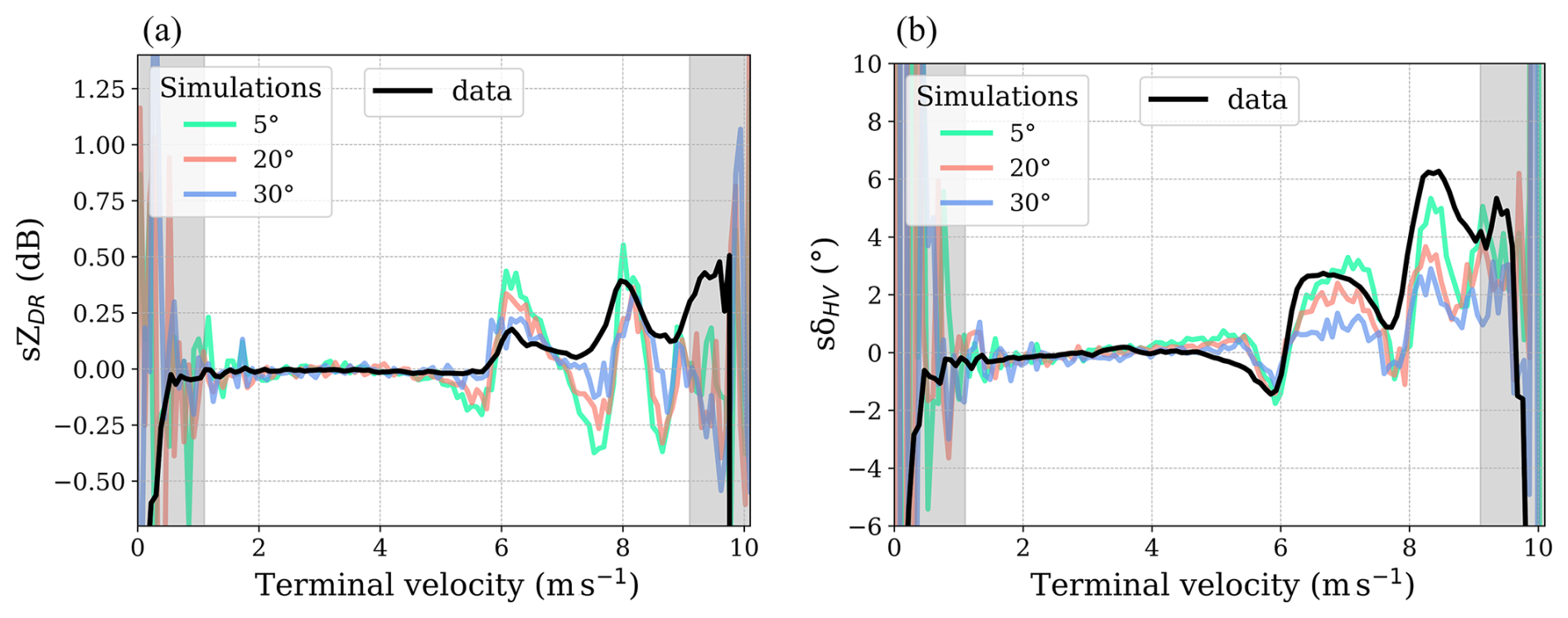
Figure 10 Spectral polarimetric variables of case study 2: (a) spectral differential reflectivity sZ_DR; (b) spectral differential phase sδ_HV. Black lines represent the measured data. Faint green, orange, and blue lines represent the simulations for different canting angle distribution widths (wobbling): 5, 20, and 30°, respectively.

In the subsequent analysis, only one simulation method is presented, as the strong agreement between the two methods is verified in the previous case (Sect. 3.1). In Fig. 10, a comparison between simulated and observed spectral polarimetric variables is presented. The simulations are generated using varying drop wobbling, represented by canting angle distribution widths of 5, 20, and 30°. The maxima and minima for the simulated variables are found to be more pronounced, relative to the measurements. There is sufficient agreement for the first notch of sδ_HV up to 5 m s⁻¹. The simulated sZ_DR exhibits a similar trend to the measurements; however, the amplitudes of the maxima are more pronounced and the minima are significantly deeper. One potential cause of these discrepancies is the assumption that drops have a spheroid shape (oblate). Therefore, it seems plausible to conclude that the T-matrix approach using spheroids is inadequate to simulate the spectral polarimetric variables of raindrops at higher frequencies, such as 94 GHz. The increasing canting of the drops in simulations (faint green, orange, and blue lines in Fig. 10) causes spectral broadening, which occurs because the wobbling of the drops averages out the distinct polarization signals over a wider range of velocities. The sZ_DR values are spread over a wider range of Doppler velocities, reducing the sharpness of the extrema. The more uniform distribution of drop orientations smooths out the sZ_DR signal. Similarly, the broadening of phase differences across the spectrum leads to smeared-out minima and maxima in sδ_HV, meaning a more gradual and continuous transition in the phase difference between horizontally and vertically polarized waves. In a nutshell, increased canting causes a more isotropic distribution of drop orientations, leading to smoother, less distinct, spectral features.

4 Conclusions and ways forward

In this study, simulations of spectral polarimetric variables were compared with real measurements in rain conditions for different levels of turbulence. The simulation accounts for such factors as the noise present in real measurements, atmospheric turbulence, and the wobbling of raindrops, aiming to replicate the complexities of actual radar data. These effects are considered to ensure a more realistic comparison between the simulated and measured spectral polarimetric variables.

The results reveal that the simulations closely align and show reasonable agreement with observations only within a limited area of the Doppler spectrum, approximately to terminal velocities up to 5 and 7 m s⁻¹ (i.e., equi-volume diameters smaller than 1.33 and 2.25 mm), respectively. Overall, the positions of the notches in the simulations align well with the observations, indicating that the velocity distribution and the location of the resonances are properly captured by the simulations. However, the amplitudes of the notches are not accurately represented. Notably, the simulations more accurately fit the maxima, compared with the minima, especially for the differential phase. The minima in the measured data of both sZ_DR and sδ_HV appear muted, while the simulated minima are significantly deeper. The maxima and minima differences are stronger in the case of lower turbulence conditions.

These discrepancies pinpoint potential limitations in the model's treatment of the amplitude modulation caused by scattering. A potential explanation may lie in the assumption used in the T-matrix approach, which models raindrops as spheroids or, more generally, as rotationally symmetric particles. However, raindrops undergo oscillations (Szakáll et al., 2010); thus, they may not be characterized by rotational symmetry. This suggests that traditional methods for computing scattering properties, such as the well-established T-matrix method, may produce inaccurate scattering parameters, especially for resonant particles (i.e., when the radar wavelength becomes comparable to or smaller than the raindrop size). Other more accurate methods should be used, e.g., the discrete dipole approximation or method of moments in the surface integral equation approach, as proposed in Thurai et al. (2014) and Manić et al. (2018). Future work should explore whether such more-sophisticated scattering models can indeed explain the observed discrepancies. Otherwise, data acquired in low-turbulence conditions can be used to build look-up tables of the polarimetric scattering properties for any given incidence angle in a data-driven approach, as recently proposed by Myagkov et al. (2025).

This work paves the way toward using spectral polarimetric observations of millimeter radar for testing scattering computations of rain polarimetric variables. As such, it contributes to the broader scientific community's efforts to improve cloud radar simulations and advance our knowledge of cloud processes and their implications for atmospheric dynamics.