Evaluating the feasibility of using downwind methods to quantify point source oil and gas emissions using continuously monitoring fence-line sensors

The dependable reporting of methane (CH₄) emissions from point sources, such as fugitive leaks from oil and gas infrastructure, is important for profit maximization (retaining more hydrocarbons), evaluating climate impacts, assessing CH₄ fees for regulatory programs, and validating CH₄ intensity in differentiated gas programs. Currently, there are disagreements between emissions reported by different quantification techniques for the same sources. It has been suggested that downwind CH₄ quantification methods using CH₄ measurements on the fence line of production facilities could be used to generate emission estimates from oil and gas operations at the site level, but it is currently unclear how accurate the quantified emissions are. To investigate the accuracy of downwind methods, this study uses fence-line simulated data collected during controlled-release experiments as input for a non-standard closed-path eddy covariance (EC), the Gaussian plume inverse model (GPIM), and the backward Lagrangian stochastic (bLs) model in a range of atmospheric conditions. This study's EC attempt was unsuccessful due to data collection and instrumentation issues, resulting in invalid results characterized by underestimated emissions, large negative fluxes, and cospectra/ogives that deviated from their ideal shapes. Consequently, the EC results could not be compared with the GPIM and bLS model. The bLs model demonstrated the highest accuracy for single-release single-point emissions, though it exhibited greater uncertainty than GPIM under multi-release conditions. Across the GPIM and bLs model, the most reliable quantification was achieved with 15 min averaging and a narrow 5° wind sector range. Although EC was limited in this context, future studies should consider employing a standard EC system and further optimizing GPIM and bLs approaches – particularly for complex multi-source scenarios – to enhance quantification accuracy and reduce uncertainty.

1 Introduction

Reducing methane (CH₄) emissions from oil and gas systems is necessary for adhering to regulations and voluntary reporting frameworks such as the Oil & Gas Methane Partnership 2.0 (OGMP 2.0) (UNEP, 2024). The OGMP 2.0 provides a comprehensive measurement-based international reporting framework allowing companies to stay ahead of regulatory compliance requirements, meet investor and market pressure, have an enhanced corporate image, and prevent revenue loss by lowering their emissions. In the US, the amount of CH₄ emitted from US oil and gas production is currently compiled by the US Environmental Protection Agency (EPA) under Subpart W. Typically, companies use a bottom-up inventory approach where emission factors (CH₄ emissions per equipment, e.g., separator, or emissions per event, e.g., liquid unloading) are multiplied by activity factors (total number of pieces of equipment or events; US EPA, 2023) to generate emissions. This quantification approach has several shortcomings: (1) it calculates CH₄ emissions separately for natural gas and petroleum systems, which are practically not independent systems and can result in bias based on changes in gas to oil ratios throughout a basin (Riddick et al., 2024a); (2) some emission factors used are outdated (Riddick et al., 2024b), while others do not account for the temporal and spatial variations in emissions (Riddick and Mauzerall, 2023); (3) emission factors do not account for long-tail distributions (Riddick et al., 2024b); (4) there is difficulty in obtaining a truly representative sample from a large, diverse population to generate emission factors (Allen, 2014); and (5) possibly unreliable data are reported by operators (Chan et al., 2024). Recently, mechanistic models, such as the Mechanistic Air Emissions Simulator (MAES), have been developed to address shortcomings in bottom-up CH₄ reporting (Mollel et al., 2025), but these still depend on direct measurements to inform emission factors.

Top-down methods, including using aircraft such as Bridger Photonics light detection and ranging (lidar; 90 % detection limit of ∼ 2 kg h⁻¹) (Johnson et al., 2021) and satellites such as Carbon Mapper (predicted 90 % detection limit of about 100 kg h⁻¹) (Carbon Mapper, 2025), can also be used to infer emissions. However, these survey methods only quantify emissions over a very short period of time (< 10 s), and observations are typically made during the day, which can often coincide with maintenance activities that can bias emissions and result in overestimation (Riddick et al., 2024a; Zimmerle et al., 2024). Additionally, different top-down technologies measuring the same source have disagreed on their reported emissions, which has called into question the credibility of these methods (Brown et al., 2023; Conrad et al., 2023). As a result, ensuring accuracy in models and technologies used in CH₄ emissions quantification has been a complex issue.

Currently, fence-line methods are used to detect, localize, and quantify emissions. This approach uses point sensors fixed to the fence line of a production site, with emissions detected when the measured concentration exceeds a threshold, localized by triangulating multiple detections and quantified using a simple dispersion modeling framework, usually based on a Gaussian plume inverse approach (Bell et al., 2023; Day et al., 2024; Riddick et al., 2022a). Detection and localization of simulated fugitive emissions using this approach have been successfully demonstrated in controlled-release studies. For example, Ilonze et al. (2024) reported a 90 % probability of detection for emissions between 3.9 and 18.2 kg CH₄ h⁻¹ using multiple point sensors and scanning/imaging systems. However, significant uncertainty in quantification remains; their study reported emissions being incorrectly estimated by a factor of 0.2 to 42 for releases between 0.1 and 1 kg CH₄ h⁻¹ and by a factor of 0.08 to 18 for emissions above 1 kg CH₄ h⁻¹. While informative, the methods in Ilonze et al. (2024) differ in key ways from those employed here – specifically, their use of multiple sensors and a distributed monitoring configuration as opposed to the single-instrument, fence-line-based framework used in our study – limiting direct comparison of quantification accuracy. This study evaluates the quantification accuracy of the closed-path eddy covariance (EC), the Gaussian plume inverse model (GPIM), and the backward Lagrangian stochastic model (bLs) for oil and gas point source quantification using a single instrument deployed at a fence-line distance.

Eddy covariance is a vertical flux gradient measurement that measures CH₄ emissions based on the covariance between CH₄ concentrations measured using a fast-response analyzer (> 10 Hz) and a vertical wind vector measured by a fast-response sonic anemometer (> 10 Hz) (Fig. 1; Morin, 2019). It is typically implemented over long, homogeneous fetches where the eddy mixing scale is a small fraction of the distance from the site, providing more predictable vertical transport. Dumortier et al. (2019) used EC to estimate known point source emissions at a cow's muzzle height and reported that the model could estimate emissions between 90 % and 113 % of the true emissions. Dumortier et al. (2019) stated that the optimal controls for point source quantification and footprint modeling involve using running means with 15 min averaging periods, not applying the Foken and Wichura (1996) stationarity filter, and using the Kormann and Meixner (2001) footprint function. The study tested the model using an artificial CH₄ source at 0.8 m, programmed to emit when winds came from the source direction (±45°) and when friction velocity (u_∗) was above 0.13 m s⁻¹. In the point source testing of Dumortier et al. (2019), they noted that amplitude resolution, skewness, and kurtosis tests were disabled as they deleted almost all periods involving the artificial source in the footprint. Rey-Sanchez et al. (2022) studied the accuracy of the Hsieh model (Hsieh et al., 2000), the Kljun model (Kljun et al., 2015), and the K&M model (Kormann and Meixner, 2001) in calculating the footprint of point source hot spots using footprint-weighted flux maps. The study reported the K&M model to be the most accurate. Polonik et al. (2019) compared five gas analyzers, two open-path analyzers, two enclosed-path analyzers, and one closed-path analyzer for carbon dioxide EC measurements. The study noted that while open-path sensors minimize spectral attenuation and require smaller spectral correction factors compared to sensors with an inlet tube such as a closed-path sensor, open-path sensors risk data loss in non-ideal conditions like precipitation, fog, dust, or dew. The main challenge of applying EC to continuous monitoring of oil and gas sites is instrument limitations (it requires deployment of multiple sensors throughout a facility; sensor cost is a factor), statistical tests, and quality controls, all of which could filter out some of the data.

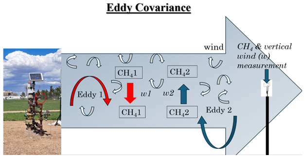
Figure 1 Illustrations of eddy covariance, where CH₄ is methane concentrations, and w is vertical wind speed.

The GPIM method calculates the CH₄ emission rate as a function of mole fraction at a point in space ($x,y,z$), downwind distance, perpendicular (crosswind) distance, mean wind speed, and atmospheric stability (Fig. 2a, Riddick et al., 2022b). This method has been used to quantify emissions from oil and gas production sites, especially for survey solutions (Riddick et al., 2022b). For a single point source, Riddick et al. (2022b) reported absolute uncertainties of between 40.7 % and 60 % in a controlled-release experiment involving 10 replicate measurements of compressed natural gas (1.5 m release height), with concentrations measured using a mobile vehicle survey. While this differs from continuous fence-line deployment, it offers insight into the inherent uncertainty in the GPIM method in field conditions. Using controlled single point source tests, Foster-Wittig et al. (2015) reported average errors of between −5 % and 6 %. The limitations of the GPIM method are that it assumes a homogeneous emission source, steady-state flow, and uniform dispersion of gas in an open area free of obstructions (Hutchinson et al., 2017).

The bLs model adapted in WindTrax can simulate the transport of gases from point sources that emit them (Fig. 2B; Crenna, 2006). The model releases individual particles and follows them along their unique paths in air by mimicking the random, turbulent motion of the atmosphere. Tagliaferri et al. (2023) investigated the validity of WindTrax in quantifying emissions from complex sources and reported the model to be reliable under neutral conditions, underestimate emission rates during unstable stratification, and overestimate emissions during stable conditions. Similarly to the GPIM method, the model assumes free flow of air in the absence of obstructions and uses time-averaged data as input.

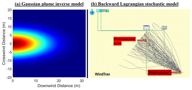
Figure 2 (a) A plume that follows a Gaussian plume inverse model, where the emission rate can be inferred from concentrations at different downwind distances and crosswind distances. (b) An illustration of how the backward Lagrangian stochastic model traces particles to the source.

Continuous monitoring of CH₄ emissions using fence-line sensors requires proper quantification of intermittent and persistent releases from oil and gas during all release (complex emission profiles) and atmospheric conditions (unstable, neutral, and stable). Oil and gas emissions are characterized by intermittent, non-uniform, and single or multiple point source emissions, varying in leak size, location, height, and distance between the source and sensor, and are typically in complex aerodynamic environments (i.e., not flat). An ideal quantification model should always quantify emissions and should capture short- and long-lasting emission events. Most models have been validated to work best during neutral conditions for single point sources. However, it is important to test and apply these models during non-neutral conditions as well, as these are part of real-world conditions where continuous monitoring is applied. In this study, we evaluate whether using a readily available CH₄ cavity ring-down analyzer for model quantification, such as the closed-path EC, is a feasible solution for quantifying point source emissions.

This study aims to inform the feasibility of downwind quantification models in oil and gas settings by investigating which models are likely to work most of the time with instrumentation that is typically available for fence-line deployment. Fence-line sensor deployments involve multiple sensors, continuously running in all conditions and providing emissions data. Using robust releases and environmental conditions, this study aims to investigate the performance of these methods in quantifying emissions for known gas release rates and evaluating uncertainties that could result in incorrect CH₄ reporting. Specifically, this study evaluates the overall quantification accuracy (linear regression slope of estimated versus actual emissions and R²) of closed-path EC, the bLs model, and the GPIM method in quantifying single-release single-point and multi-release single-point emissions that simulate oil and gas emissions.

2 Methods

2.1 Experimental setup

Controlled-release experiments were conducted at Colorado State University's Methane Emissions Technology Evaluation Center (METEC) in Fort Collins, CO (USA, ∼ 105 km north of Denver) between 8 February and 20 March 2024. METEC is a simulated oil and gas facility that does controlled testing for emissions leak detection and quantification technology development, field demonstration, leak detection protocol, and best practice development (Colorado State University, 2025a). The weather conditions during the test period were mostly sunny, but precipitation was also observed (32 sunny days, 7 snowy days, 12 rainy days, 7 cloudy days, and 1 foggy day; Sect. S1). Wind speeds were between 0 and 25 m s⁻¹, and temperatures ranged between −15 and +19 °C (Sect. S1). A stationary mast holding the instrumentation was set up on the northwest corner of METEC to take advantage of the predominant wind direction, avoid the largest aerodynamic obstructions, and simulate the likely placement of a fence-line instrument (Fig. 3A; Day et al., 2024; Riddick et al., 2022a). Fence-line sensors are typically placed within the oil and gas perimeter (∼ 30 m). This study collected data for what we considered close and far releases, with distances between 9 and 94 m.

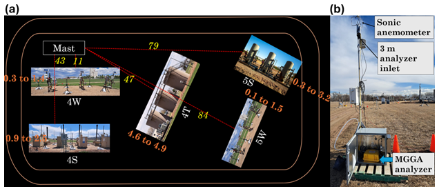
Figure 3 (a) Map illustration of major pieces of equipment and the measurement points at Colorado State University's Methane Emissions Technology Evaluation Center (METEC) in Fort Collins, CO, USA. Equipment 4S denotes horizontal separators, 4W is wellheads, 4T is tanks, 5S is vertical separators, and 5W is wellheads. Panel (b) is the measurement point for the microportable greenhouse gas analyzer for the closed-path eddy covariance, Gaussian plume inverse model, and backward Lagrangian stochastic model quantification. The inlet tubing and the sonic anemometer are at 3 m height. The dotted red lines with yellow numbers show the average distances (meters) between the emission equipment and measurement point. The orange numbers show the range of emission heights (meters) for each equipment piece. The analyzers were hosted in a temperature-controlled box.

Methane concentration data for the closed-path EC, GPIM, and bLs methods were collected through an inlet tubing (3.275 mm inner diameter) at 3 m height, connected to the ABB (Zurich, Switzerland) GLA131 Series microportable greenhouse gas analyzer (MGGA) set to sample at 10 Hz. The MGGA is a closed-path greenhouse gas analyzer with a ∼ 3.2 L min⁻¹ pump flow rate, 10 cm cell length, 2.54 cm cell diameter (∼ 0.23 sccm (standard cubic centimeters per minute) effective volume), and 0.4 s gas flow response time. The inlet tubing was collocated with an R. M. Young (Traverse City, MI, USA) 81000 sonic anemometer, which measured micrometeorology at 10 Hz (Fig. 3B). The northward, eastward, and vertical separation of the inlet tubing from the sonic anemometer was 0, 0, and −10 cm, respectively.

2.2 Controlled methane releases

Controlled releases were part of the METEC Spring 2024 Advancing Development of Emissions Detection (ADED) campaign conducted between 6 February and 29 April 2024 (Colorado State University, 2025b). Natural gas of known CH₄ content was released from above-ground emission points attached to equipment typically present in an oil and gas facility (tanks, separators, and well pads). The gas release rates ranged between 0.01 and 8.7 kg h⁻¹, and the release durations ranged from 10 s to 8 h, simulating both fugitive emission and large-emission events. The releases were run during both the day and the night. The distance from the release points to the measurement points ranged between 9 and 94 m, and emission heights were between 0.1 and 4.9 m (Fig. 3A). Emission points simulate the realistic size and locations of typical emissions from components such as the thief hatches, pressure relief valves, flanges, bradenheads, pressure transducers, Kimray valves, and vents. The releases included both single-point emission (single releases) and multi-point emission events (multiple simultaneous releases).

2.3 Calculation of roughness length

Surface roughness length (z₀) was calculated from friction velocity (Sect. S2.1: Eqs. S1 and S2) by splitting the high-frequency sonic anemometer data into 15 min tables and filtering for those in neutral conditions, | L | > 500 (Sect. S2.1: Eq. S3). The overall roughness length selected as the median of all the calculated z₀ was 0.1 m (Rey-Sanchez et al., 2022).

2.4 Model quantification

2.4.1 Eddy covariance

Data pre-processing

Evaluating the MGGA CH₄ data showed that actual sampling was between 4 and 12 Hz (majority of the data collected at approximately 6 Hz), even though the analyzer had been configured to sample at 10 Hz (Sect. S2.2). To account for this sampling variability, data were filtered to when sampling was equal to or greater than 8 Hz. Data sampled at frequencies above 8 Hz were downsampled to 8 Hz. The 8 Hz frequency threshold was selected to ensure uniform sampling, provide enough data for model evaluation as most sampling was conducted at lower frequencies, and preserve as much temporal resolution as possible given the system limitations. The actual sampling frequency of the sonic anemometer meteorological data (horizontal wind vectors (u, v), vertical wind vector (w), temperature (T), and pressure (P)) varied between 7 and 9 Hz, with the most frequent frequency at 8 Hz (Sect. S2.2). As the MGGA gas analyzer and sonic anemometer were not designed to clock synchronously, using the MGGA CH₄ clock time as a reference, meteorological data from the sonic anemometer were matched to the MGGA CH₄ data using linear interpolation to generate concentration–meteorological 8 Hz data. While, under ideal circumstances of a fast pump and short tube length, correct time series matching can be achieved by establishing a clear point of maximum covariance when determining the time lag, this is difficult for our system due to a 3 L min⁻¹ pump flow rate and 3 m tubing that caused both attenuation and time lag.

The aggregated concentration–meteorological data were then merged with METEC's release data and metadata, and release event tables were created. Release event tables are aggregated tables of concentration, meteorology, and release (emission source location, duration, and rate) information for all defined release events at METEC. The concentration–meteorological–release event data were then separated into single-release and multi-release events. Single-release events occur when there is a single emission point at the site level, while multi-release events occur when there is more than one emission point at the site level. The concentration–meteorological–release event tables were split into 5, 15, and 30 min release event tables (i.e., there was continuous release during the duration). Based on the bearing of the emission point relative to the measurement point and the average wind direction during the duration, the data were further filtered to downwind data at ±10, ±20, and ±45°.

Flux calculation

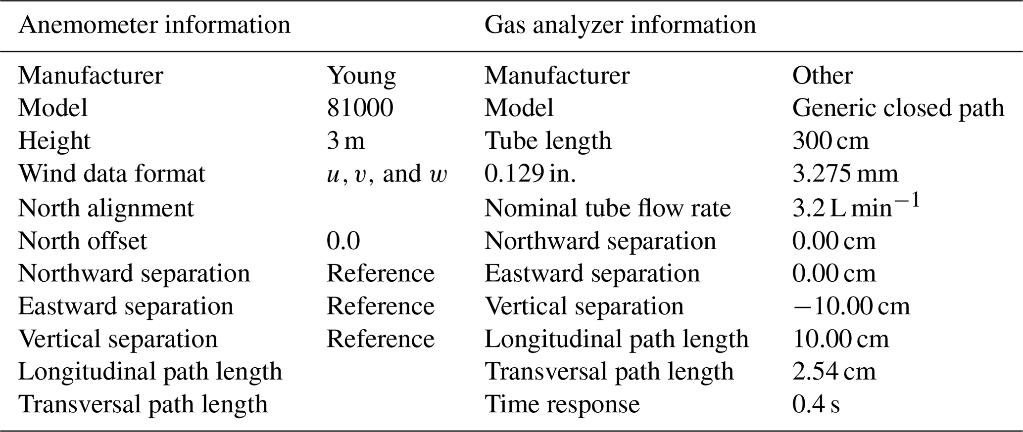
Turbulent fluxes were calculated using the open software EddyPro^® version 7 (LI-COR Biosciences, 2021). The acquisition frequency was set at 8 Hz, while the file duration and flux interval were set at 5, 15, and 30 min, respectively, depending on the files being processed. Table 1 shows the instruments that were input to the software.

Table 1 Anemometer and gas analyzer input into EddyPro.

In raw data processing, axis rotations for tilt correction under wind speed measurement offsets were selected. Under turbulent fluctuations, double-rotation and block average detrend methods were used. Covariance maximization with default settings was used for time lag detection; time lag detection was enabled. Compensation for density fluctuations (Webb–Pearman–Leuning terms) (Webb et al., 1980) was disabled as the MGGA analyzer reported dry CH₄, water mole fractions, cell temperature, and pressure synchronously. Mauder and Foken (2004) (0–1–2 system) were used for the quality check. All statistical tests for raw data screening (Vickers and Mahrt, 1997) – spike count/removal, amplitude resolution, dropouts, absolute limits, skewness and kurtosis, discontinuities, time lags, angle of attack, and steadiness of horizontal wind – were selected. The default values for all these tests were used. Similarly, default settings for spectral analysis and corrections were used. Analytic corrections of high-pass-filtering effects (Moncrieff et al., 2005) for the low-frequency range and correction of low-pass-filtering effects (Fratini et al., 2012, in situ analysis and instrument separation; Horst and Lenschow, 2009, only crosswind and vertical) in the high–frequency range were used.

Post-processing

Flux data were flagged as “2”, low quality, based on Mauder and Foken's (2004) (0–1–2) quality system. Cospectral analysis revealed that the EC system in this study smoothed out low-frequency eddies, as the cospectra lacked the ideal shape characterized by a low-frequency rise, a peak region, and a high-frequency decay (Sect. S2.3.1). While the slope in the high-frequency region varies around the theoretical $-\mathrm{4}/\mathrm{3}$ slope, the cospectral data followed the 1:1 line, indicating a consistent spectral shape across sampling periods. We also examined the relationship between CH₄ flux and friction velocity (u_∗) to identify a u_∗ threshold below which flux estimates may be unreliable (Sect. S2.3.2). However, no consistent relationship was observed across atmospheric stability classes (unstable, stable, and neutral). CH₄ fluxes varied widely – including both positive and negative values – across the full range of u_∗ (∼ 0 to 1 m s⁻¹), with no discernible threshold beyond which fluxes stabilized. This indicated that CH₄ fluxes were effectively independent of u_∗, and thus, data from all u_∗ values were retained. Ogive analysis was conducted to assess whether averaging durations of 5, 15, and 30 min were sufficient for capturing the full turbulent flux. The resulting ogive curves deviated from the ideal asymptotic shape, particularly at the highest and lowest frequencies (Sect. S2.3.3). Notably, the curves did not exhibit a clear plateau near the low-frequency end, where the cumulative flux should approach unity. This indicates incomplete flux capture. Furthermore, the similarity in ogive shapes across different frequencies – mirroring patterns seen in the cospectra – suggests a lack of significant turbulent contributions and the influence of non-turbulent, possibly advective processes. These results imply that the EC system may not have fully resolved the flux due to insufficient averaging time, non-stationarity, or instrument-related limitations (Sect. S2.3.4). As positive fluxes are generally considered emissions and negative fluxes depositions, data were further filtered for positive fluxes, which were then quantified to emission rates.

Footprint calculation

Eddy covariance footprints were calculated using the Kljun et al. (2015) and Kormann and Meixner (2001) footprint models. For the Kljun et al. (2015) model, the free online MATLAB code of the model was used, while the Kormann and Meixner (2001) model was coded in MATLAB. To determine the point source footprint contribution, the study first calculated the area that contributed 90 % of the vertical flux, and based on the location (x and y coordinates based on wind direction and distance from the source) of the point source, the source was determined if it was within the 90 % footprint area. Point source emissions of sources within this region were then calculated based on the approach by Dumortier et al. (2019). This approach assumes that all measured fluxes are equal to fluxes resulting from a single point source. In the case of the mast being downwind of more than one source, more sonic anemometers are needed to solve the two unknown point source fluxes.

2.4.2 Gaussian Plume inverse method

Data pre-processing

Methane concentration data from the MGGA analyzer and meteorology data from the sonic anemometer were averaged to 1 Hz and aggregated. The aggregated concentration–meteorological data were merged with METEC's release data and metadata, and release event tables were created. The concentration–meteorological–release event data were then separated into single-release and multi-release events. For single-release events, the concentration–meteorological–release event tables were split into 5, 15, and 30 min release event tables. Based on the bearing of the emission point relative to the measurement point and the average wind direction during the duration, the data were further filtered to downwind data within ±5, ±10, and ±20° wind sector ranges. Multi-release events were further classified into multi-release single-point emissions (i.e., there were multiple emissions at the site level, but the mast was downwind of a single source) and multi-release multi-point emissions (i.e., there were multiple emissions at the site level, and the mast was downwind of more than one source). This study focuses on single-release single-point and multi-release single-point emissions. For continuously monitoring sensors, background concentration can be determined from CH₄ concentrations measured by a sensor upwind of the emission source or by sampling when the wind blows away from the source. However, for continuously monitoring sensors, using an upwind sensor has the limitation of missing downwind background noise resulting from emissions in the preceding emission event where there is residual CH₄ in air, especially during stable conditions, and capturing sensors drift in the downwind sensor. In this study, background CH₄ was calculated as the average of the lowest 5th percentile, 5 min before each release started. In cases where this background was greater than the mean CH₄ concentration in the quantifying duration, the minimum CH₄ concentration for that duration was used as the background. Methane enhancement was then calculated as CH₄ concentration minus the background.

Quantification

The GPIM was evaluated under six scenarios (two equations and three different dispersion coefficient generations) using single-release single-point emissions to test when the model works best (Sect. S2.1: Eqs. S7 and S8). Dispersion coefficients were generated based on (1) high-frequency sonic anemometer data at ∼ 10 Hz, (2) EPA point source dispersion coefficients (US EPA, 2013), and (3) 1 Hz sonic anemometer data. The scenario with the slope closest to 1 and the highest R² across averaging durations and wind sector ranges was selected and used for multi-release single-point emissions quantification. For single-release tables, the measurement point was downwind of a single source (single-release single-point emission); hence the tables were quantified as they were. However, for multi-release events, the tables were further processed as the GPIM method is designed to quantify one point source at a time. For multi-release events, the number of emission points in the downwind tables was used to further classify the tables into multi-release single-point emissions (i.e., there were multiple emissions at the site level, but the mast was downwind of a single source) and multi-release multi-point emissions (i.e., there were multiple emissions at the site level, and the mast was downwind of more than one emission source). The GPIM method was only used for multi-release single-point emissions.

2.4.3 Backward Lagrangian stochastic model

Pre-processed data from the GPIM method were used for bLs quantification. Quantification was done using the open-source software WindTrax 2.0 (Crenna, 2006; WindTrax 2.0, 2020). For every 5, 15, and 30 min duration within ±5, ±10, and ± 20°, respectively, inputs included roughness length (z₀); Monin–Obukhov length (L – Sect. S2.1: Eq. S3); mean wind speed, wind direction, concentration, pressure, and temperature; background concentration; source height; and distance from the emission point to the sensor. WindTrax is also designed to quantify a single point source at a time and was hence only used to quantify single-point single emissions and multi-point single emissions.

3 Results

3.1 Eddy covariance

3.1.1 Single-release single-point emissions

For single-release single-point (SRSP) emissions, the closed-path EC underestimated emissions. Using the Kljun et al. (2015) footprint model, the slope of the linear regression between estimated emissions and actual emissions ranged from −0.03 to 0.54 at 5 min, from −0.36 to −0.04 at 15 min, and was 0.03 at 30 min for 45° (10 and 20° had insufficient data points) (Fig. 4). The adjusted R² was between −0.06 and 0.12, indicating no linear relationship between the estimated and actual emissions (Fig. 4). Using the Kormann and Meixner (2001) footprint model, the slope was between −0.42 and 0.17 at 5 and 15 min, respectively, and −0.08 at 30 min for 45° (Sect. S3.1.1). Similarly, the adjusted R² values were between −0.07 and 0.05. These results indicate that this study's EC system using either the Kljun et al. (2015) or the Kormann and Meixner (2001) footprint model did not reliably quantify emissions for SRSP cases. The low slopes and adjusted R² values suggest little to no linear relationship between estimated and actual emissions under the tested conditions (Fig. 4; Sect. S3.1.1).

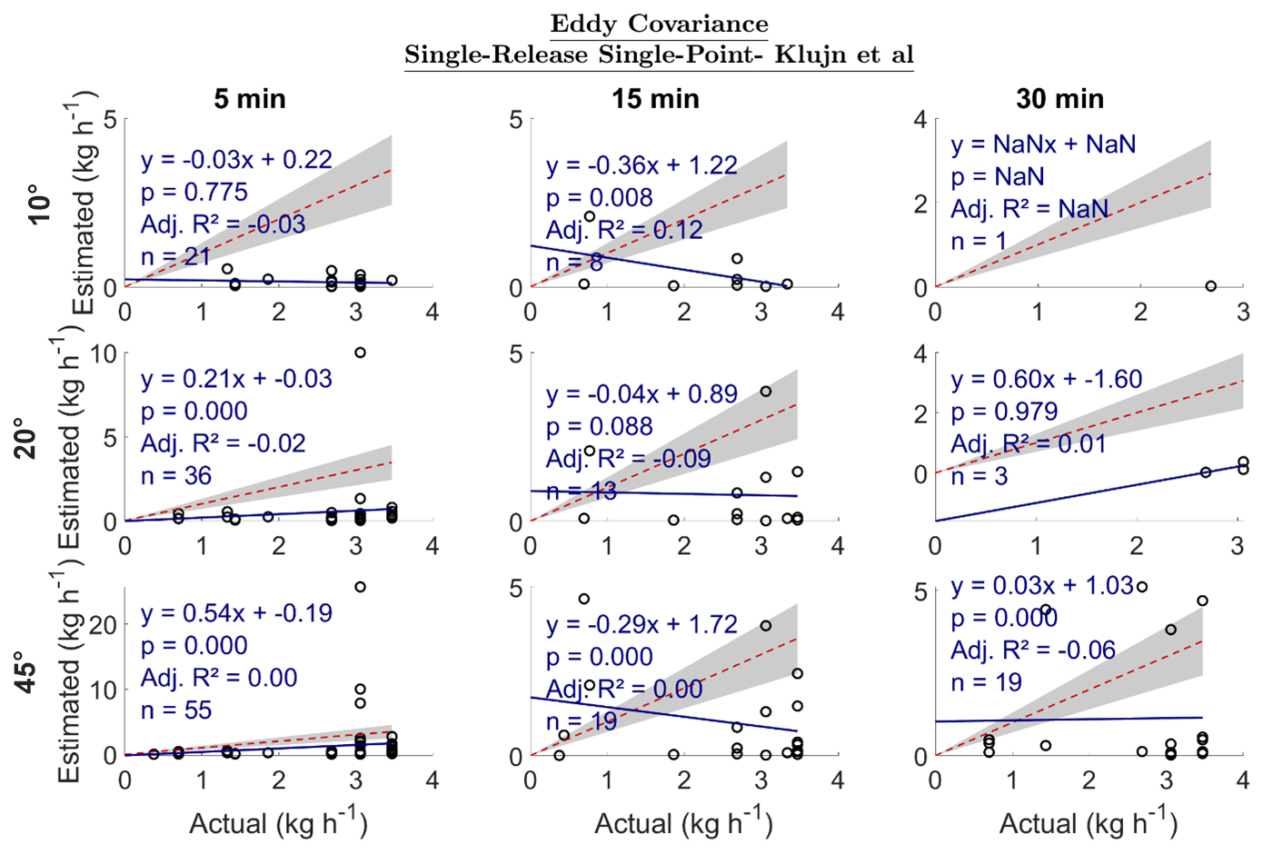
Figure 4 Estimated emission vs. actual emission (kg h⁻¹) for single-release single-point emissions. The dotted red line is a 1:1 line based on actual emissions; i.e., points below the line are underestimated emissions, and those above are overestimated emissions. The gray region represents ±30 % of the actual emissions. Adj. R² is the adjusted R². The sample size is n.

3.1.2 Multi-release single-point emissions

For multi-release single-point (MRSP) emissions, the closed-path EC largely underestimated emissions and did not show good agreement between estimated and actual emissions (Fig. 5). Using the Kljun et al. (2015) footprint model, the slope was between −0.51 and 0.18, except for the 5 min 45° category that had a slope of 0.61. The adjusted R² did not show a linear relationship between estimated and actual emissions, with values ranging between −0.02 and 0.00 (Fig. 5). Using the Kormann and Meixner (2001) footprint model, the slope was between −0.03 and 1.06, with good agreement of 1.06 at 30 min for 45° with an adjusted R² of 0.12 (Sect. S3.1.2). The rest of the categories had an R² of between −0.02 and 0.06. These results suggest that the EC system did not reliably quantify emissions for MRSP cases under most conditions. Only one category (30 min at 45° using the Kormann and Meixner, 2001, footprint model) showed moderate agreement (slope = 1.06, adjusted R²= 0.12), but even this explains only a small portion of the variability in actual emissions. Overall, the adjusted R² values across scenarios (−0.02 to 0.12) indicate a weak or no linear relationship.

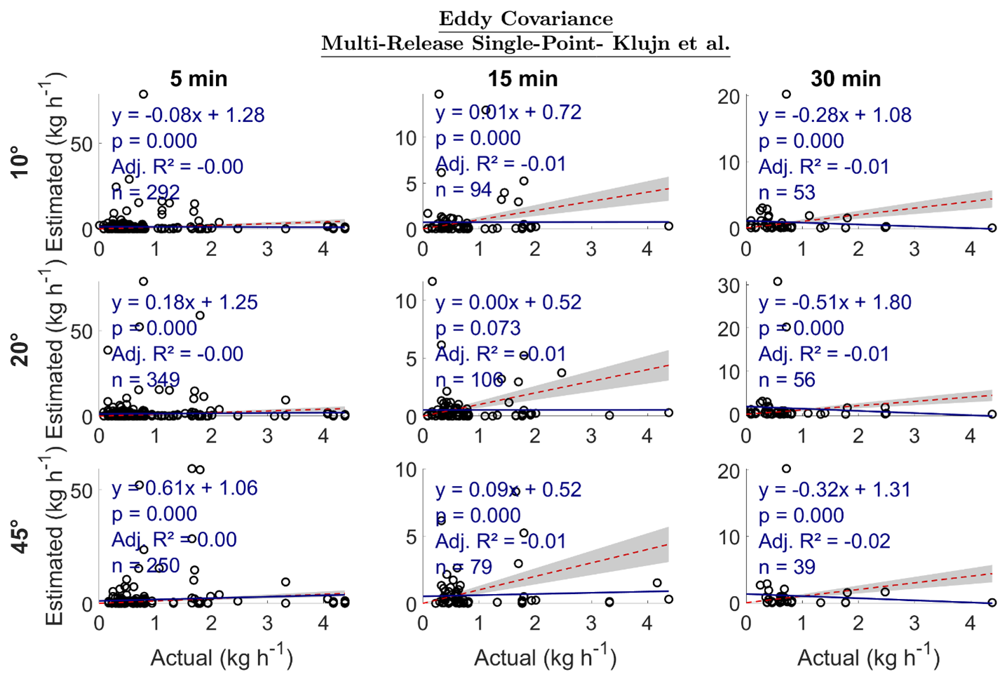
Figure 5 Estimated emission vs. actual emission (kg h⁻¹) for multi-release single-point emissions. The dotted red line is a 1:1 line based on actual emissions; i.e., points below the line are underestimated emissions, and those above are overestimated emissions. The gray region represents ±30 % of the actual emission. Adj. R² is the adjusted R². The sample size is n.

3.2 Gaussian plume inverse method

3.2.1 Single-release single-point emissions

The GPIM sensitivity analysis comparing different equations and dispersion coefficients showed no difference in quantified emissions between Eqs. (S7) and (S8). Among the dispersion coefficient sets tested (US EPA, 2013), the coefficients resulted in the most consistent performance, with the least variability in slope and the highest overall adjusted R² values (Sect. S3.2). For this scenario, the slope ranged from 1.65 to 3.92 (excluding the 30 min 5° case due to insufficient data), and adjusted R² values ranged from 0.40 to 0.64 (Fig. 6). The 15 min 5° case had a slope closest to 1 (slope = 1.65, R²= 0.40), while the 5 min 5° case showed the strongest linear relationship overall (slope = 2.42, R²= 0.64) (Fig. 6). These results suggest that while the GPIM tends to overestimate emissions (slopes > 1), it provides relatively consistent and stronger linear agreement with actual emissions compared to the closed-path EC system tested above (Sect. 3.1).

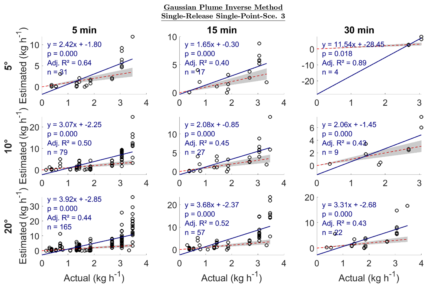
Figure 6 Estimated emission vs. actual emission (kg h⁻¹) for single-release single-point emissions. Sce.3 refers to scenario 3 of the sensitivity analysis in Sect. S3.2. The dotted red line is a 1:1 line based on actual emissions; i.e., points below the line are underestimated emissions, and those above are overestimated emissions. The gray region represents ±30 % of the actual emission. Adj. R² is the adjusted R². The sample size is n.

3.2.2 Multi-release single-point emissions

For MRSP emissions, the GPIM produced a wide range of slopes, from −43.05 to 1.60 (Fig. 7). Excluding the 5 min 5 and 10° categories and the 30 min 10° category, most other cases reported slopes between 0.76 and 1.22, suggesting potential quantification within ∼ 25 % of the actual emissions. However, the adjusted R² values in these cases were close to 0, indicating no consistent linear relationship between estimated and actual emissions (Fig. 7). This lack of correlation is likely due to the high variability in GPIM estimates, which reached up to 200 kg h⁻¹ for the selected categories, despite actual emissions being only around ∼ 6 kg h⁻¹. These results indicate that while the GPIM sometimes produced slope values suggesting close agreement with actual emissions, the lack of linear correlation and large overestimations highlight its limited reliability in quantifying MRSP emissions accurately.

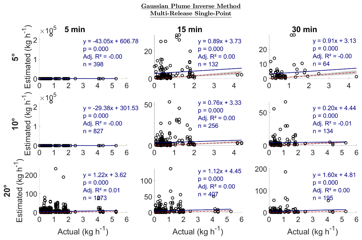
Figure 7 Estimated emission vs. actual emission (kg h⁻¹) for multi-release single-point emissions. The dotted red line is a 1:1 line based on actual emissions; i.e., points below the line are underestimated emissions, and those above are overestimated emissions. The gray region represents ±30 % of the actual emission. Adj. R² is the adjusted R². The sample size is n.

3.3 Backward Lagrangian stochastic model

3.3.1 Single-release single-point emissions

For SRSP emissions, the bLS method generally produced the most accurate slopes (i.e., closest to 1) compared to the EC and GPIM methods (Fig. 8). The 15 min 5 and 10° categories yielded the most accurate estimates, with slopes of 1.05 and 1.10, respectively. The adjusted R² ranged from 0.48 to 0.66 for the 5 min averaging duration and from 0.40 to 0.48 for the 15 min duration. At the 30 min averaging duration, performance improved in the 10 and 20° categories, likely due to increased sample sizes (Fig. 8). These results show that bLs is more suitable for quantifying single-release single-point emissions.

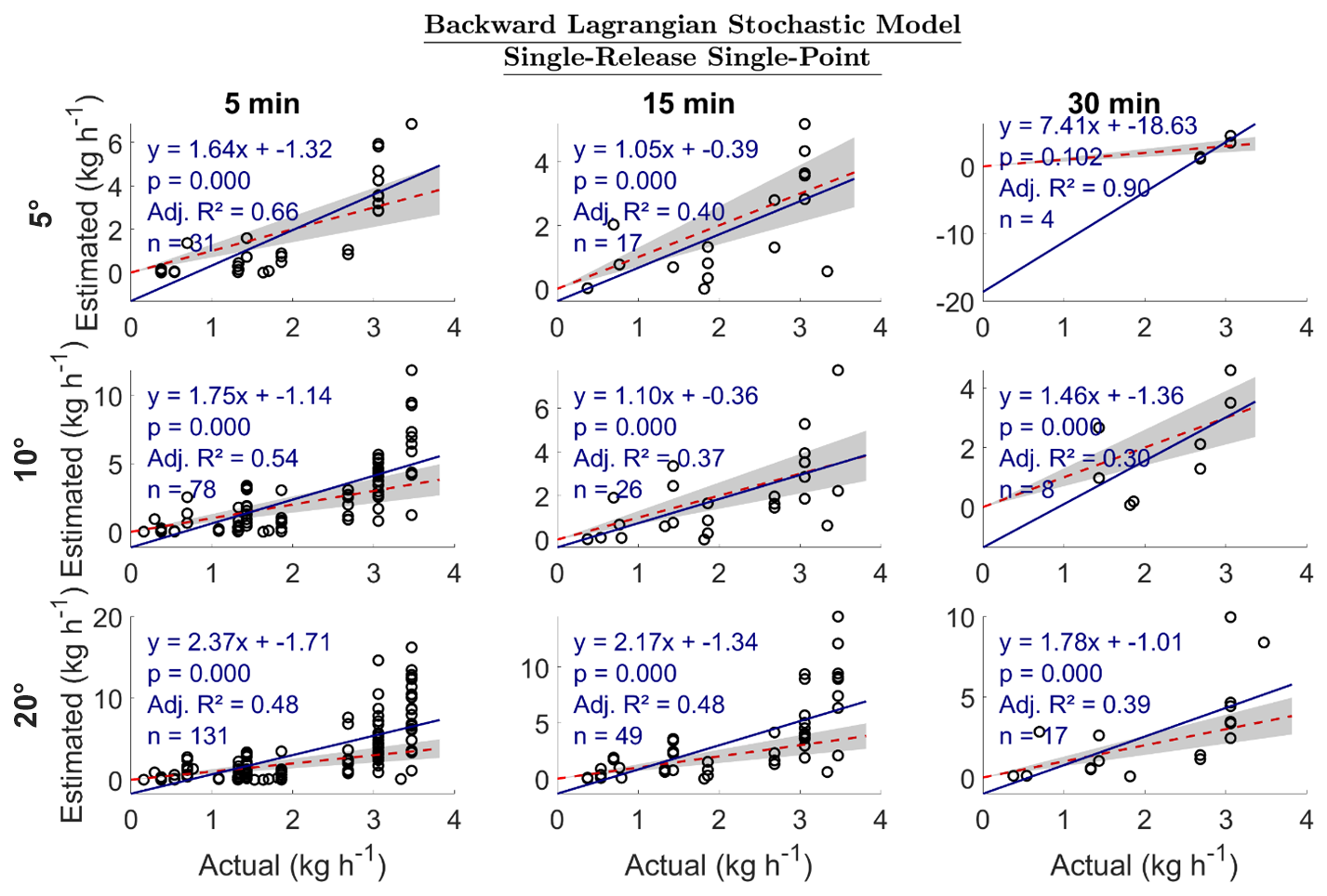
Figure 8 Estimated emission vs. actual emission (kg h⁻¹) for single-release single-point emissions. The dotted red line is a 1:1 line based on actual emissions; i.e., points below the line are underestimated emissions, and those above are overestimated emissions. The gray region represents ±30 % of the actual emission. Adj. R² is the adjusted R². The sample size is n.

3.3.2 Multi-release single-point emissions

The bLs method had large uncertainties for MRSP emissions, especially in the 5 min 5 and 10° categories (Fig. 9). In the other categories, the slopes were between −0.03 and 0.45, with an R² value of ∼ 0. Even though the estimated emissions spanned up to > 20 kg h⁻¹, mostly for actual emissions of up to 6 kg h⁻¹, many points were concentrated close to 0. Compared to the GPIM MRSP results, even though both models have an R² of ∼ 0, the GPIM had a slope closer to 1 in the 15 min category than the bLs, showing better performance. These results show that the bLs is more suitable for quantifying SRSP emissions than MRSP emissions.

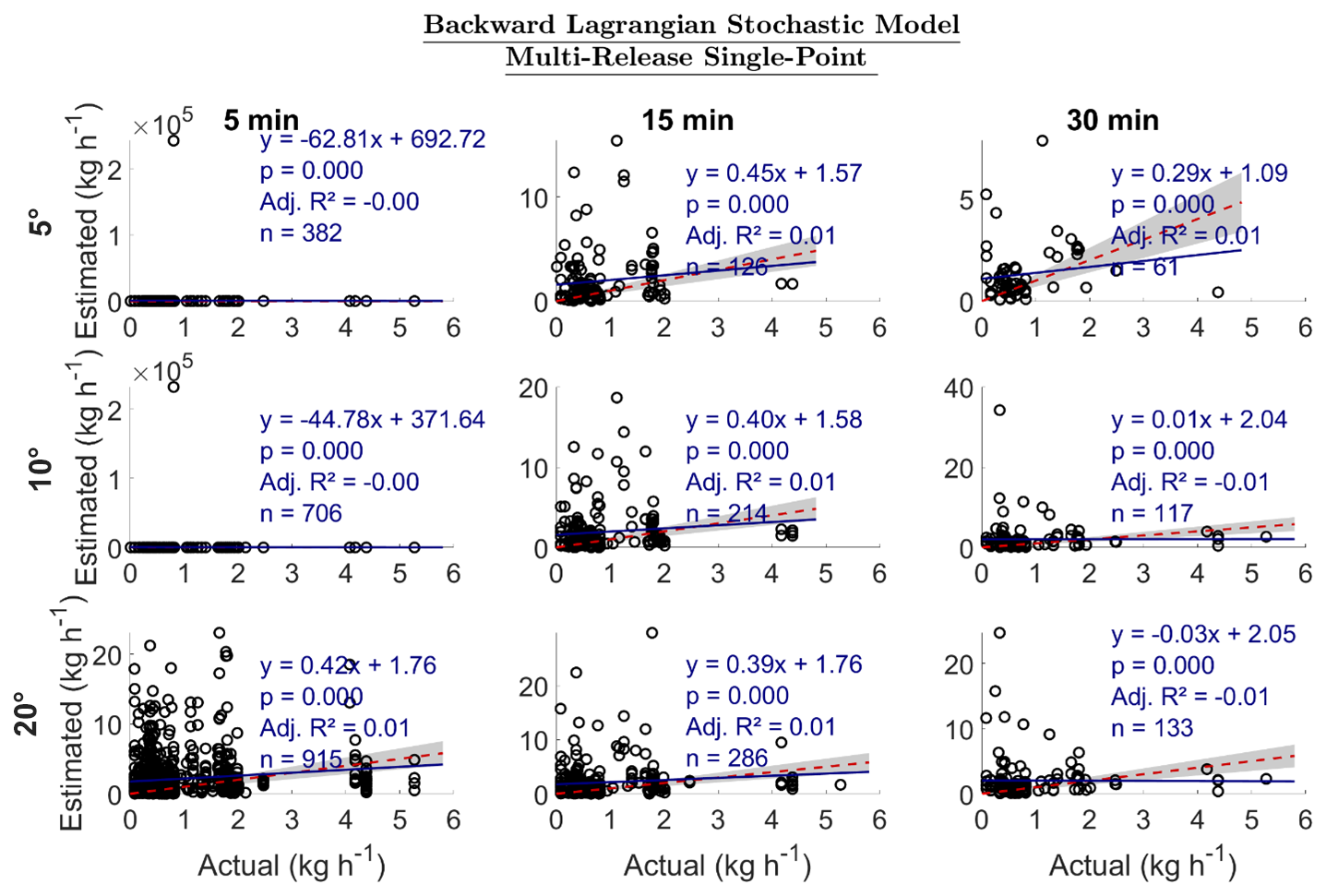
Figure 9 Estimated emission vs. actual emission (kg h⁻¹) for multi-release single-point emissions. The dotted red line is a 1:1 line based on actual emissions; i.e., points below the line are underestimated emissions, and those above are overestimated emissions. The gray region represents ±30 % of the actual emission. Adj. R² is the adjusted R². The sample size is n.

3.4 Model comparison – subset data

Using a subset of the data (SRSP), filtered by 15 min intervals within a 10° wind sector range where each model provided an emission estimate, the bLs model exhibited the best performance, with its linear regression closely aligned with the 1:1 line (Fig. 10). The slope of the regression line for the GPIM was 1.6, indicating an overestimation, while the bLs had a slope of 0.95, suggesting high accuracy. In contrast, the EC model produced slopes of 0.08 and 0.10 when using the Kormann and Meixner (2001) and Kljun et al. (2015) footprint parameterizations, respectively, indicating significant underestimation. When emission estimates were categorized by emission point, the GPIM notably overestimated emissions at locations 4W-22 and 4W-51 (identified in Fig. 3), both situated approximately 10 m from the measurement location. The EC model consistently underestimated emissions across all sources, while the bLs (WindTrax) model provided estimates closest to the expected values. The EC model produced negative emission rates associated with negative fluxes during periods of high non-stationarity (Sect. S2.3.4). These deviations from stationarity reflect intermittent plume capture, where the EC system alternated between sampling emitting and non-emitting regions. Overall, these findings indicate that for source–receptor distances ranging from approximately 10 to 90 m, the bLs model demonstrated the highest accuracy in quantifying emissions.

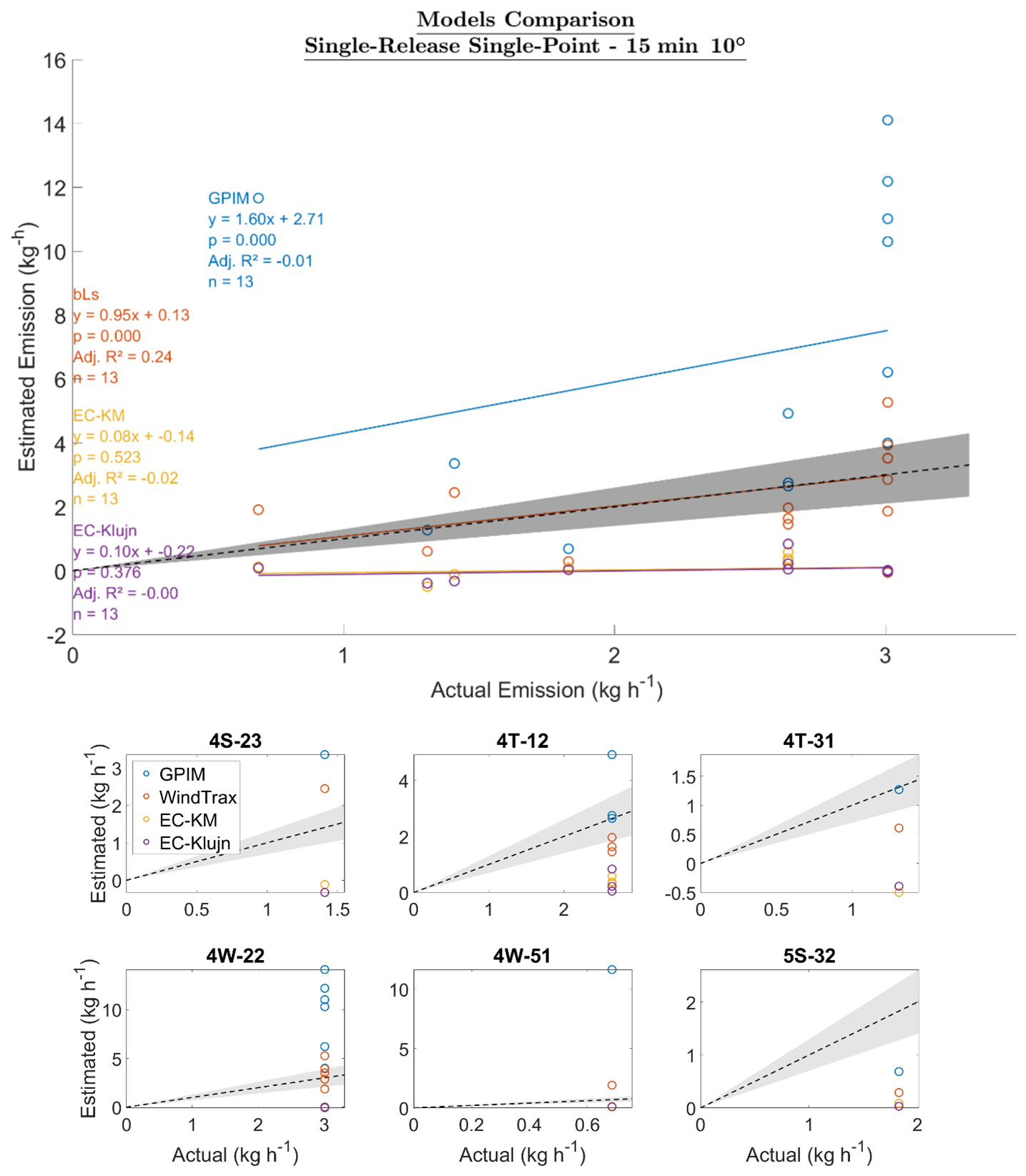
Figure 10 Top plot: estimated emission vs. actual emission (kg h⁻¹) for each model. GPIM is the Gaussian plume inverse model, bLs is the backward Lagrangian stochastic model, EC-KM is eddy covariance with the Kormann and Meixner (2001) footprint, and EC-Klujn is the eddy covariance estimate using the Kljun et al. (2015) footprint. The dotted black line is a 1:1 line based on actual emissions; i.e., points below the line are underestimated emissions, and those above are overestimated emissions. The gray region represents ±30 % of the actual emission. Adj. R² is the adjusted R². The sample size is n. Bottom plot: estimated emission vs. actual emission categorized by emission point, as illustrated in Fig. 3.

3.5 Traceability example

To illustrate how raw data were converted into model-based emission estimates, we present one representative 15 min interval used in Fig. 10. During a controlled release at point 4W-22 (wellhead), located approximately 10.5 m from the mast, the ground-truth release rate was 3 kg CH₄ h⁻¹. Over this interval, the average CH₄ concentration enhancement was 8.3 ppm above the background (determined using the 5th percentile method; see Sect. 2.4.2 “Data pre-processing”). The wind direction was 153° (0.3 m crosswind distance), with an average wind speed of 5.8 m s⁻¹. The same interval was processed through the three modeling frameworks:

• The bLs model (WindTrax), using measured concentration, geometry, and meteorological data, estimated 3.5 kg h⁻¹.

• The GPIM, using Eqs. (S7) and (S8) (Sect. S2.1) and US EPA (2013) dispersion coefficients, estimated 10.3 kg h⁻¹.

• The EC method, using the Kormann and Meixner (2001) footprint, estimated −0.004 kg h⁻¹ due to a negative flux under high-non-stationarity conditions.

This example illustrates how the bLs model reproduced the true emission most closely, while GPIM overestimated the emission, and EC underestimated the emission. More examples of data presented in Fig. 10 are available under the supplementary data, “MATLAB Code & Software Configuration – Validation.xlsx”.

3.6 Eddy covariance quality assurance and control

Evaluation of the EC data revealed quality assurance and control issues that compromised both the analysis and the conclusions drawn from the EC results. The flux data were flagged as “2” (low quality) according to the 0–1–2 quality classification system of Mauder and Foken (2004), indicating that the data were not suitable for EC analysis. In EC quality assessment, both the qualitative shape of the cospectra and the quantitative slopes of selected portions are examined to determine if the data meet accepted standards. In this study, the cospectra deviated significantly from the ideal shape, indicating problems in data collection and pre-processing. Possible causes include obstructions in the testing area, misalignment between CH₄ and sonic anemometer time series (due to the absence of a reliable method for alignment), slow response time of the gas analyzer, increased lag from the 3 m inlet tubing, and inconsistent sampling frequency. Similarly, ogive analysis – used to evaluate whether the averaging time is sufficient – showed that the ogive curves did not follow the characteristic sigmoidal shape (plateauing at the y axis and at 0). The ogive shapes were similar across all averaging intervals – none plateaued sufficiently – further indicating data collection issues that invalidate the EC method for this study. For clarity and to guide future studies, Burba (2013) provides examples of ideal cospectra and ogive shapes, illustrating how these tools can be used to diagnose instrumentation and data collection problems.

4 Discussion

Methane emissions quantification from oil and gas is a complex process that involves gas emissions from different heights and locations, encounters aerodynamic obstacles of different sizes, and includes varying emissions durations, among other factors. The ability to precisely quantify emissions using data collected by a point sensor downwind of a source is directly influenced by plume dynamics. The CH₄ plume downwind of a source will change in size and shape in different atmospheric conditions, in open areas versus areas with obstacles, diurnally, and in different seasons (Casal, 2008). In this study, we evaluated the ability of downwind methods – including a non-standard closed-path EC system, the GPIM, and the bLs model – to quantify emissions from single-release and multi-release point sources. While the field measurements took place under naturally varying meteorological conditions, these were not explicitly stratified or analyzed as experimental factors. Additionally, although on-site infrastructure such as storage tanks was present, their distance from the sampling instruments (∼ 50 m) likely rendered their aerodynamic influence negligible. As such, the analysis focuses on quantification performance under realistic but uncontrolled field scenarios, without attributing model behavior to specific atmospheric or obstacle-related conditions.

4.1 Eddy covariance

Eddy covariance was tested using a closed-path analyzer and cavity ring-down spectroscopy, with a 3.2 L min⁻¹ pump flow rate and a 0.4 s gas flow response time. The closed-path EC underestimated emissions, with a linear regression slope for estimated emissions versus actual emissions of between −0.42 and 0.54 using the Kljun et al. (2015) and Kormann and Meixner (2001) footprint models, and adjusted R² was ∼ 0. (Sect. 3.1). This is a larger uncertainty in estimated emissions than that reported by Dumortier et al. (2019), who estimated emissions at between 90 % and 113 % of true emissions (∼ 1.5 kg d⁻¹), with concentrations between 2 and 3 ppm. Our study tested closed-path EC at emission rates between 0.005 and 8.5 kg h⁻¹. Notably, the results for the non-standard EC system tested in this study may not be representative of EC performance in oil and gas, as ogive and cospectra analysis indicated that the flux may not have been fully resolved due to non-stationarity and instrument-related limitations.

Our results were derived from data filtered to include only periods with sampling frequencies ≥8 Hz, which significantly reduced the number of usable emission measurements. Although the instrument was configured to sample at 10 Hz, it did not consistently achieve this rate. This discrepancy may be attributed to instrument-related factors such as the 0.4 s gas flow response time, which could delay analysis of the drawn air sample in the cavity, or the use of a 3 L min⁻¹ pump with 3 m of tubing, which reduced the effective turnover rate. The dataset used for eddy covariance evaluation was predominantly flagged as low quality (flag 2) according to the Mauder and Foken (2004) quality control test, which classifies flux data based on steady-state conditions and the presence of well-developed turbulence (flags 0 = high, 1 = intermediate, 2 = low quality). Many of the low-quality flags were likely driven by wide deviation in vertical wind speed (w) $/$ methane (CH₄) stationarity, reflecting intermittent plume capture, where the EC system alternated between sampling emitting and non-emitting regions. The EC model produced negative emission rates associated with negative fluxes during periods of high non-stationarity (Sect. S2.3.4).

Despite high non-stationarity that resulted in low-data-quality issues, further resulting in EC inaccuracies, this study acknowledges our design limitations. Our study did not have a reliable method for aligning the asynchronous CH₄ and sonic anemometer data streams, which likely introduced substantial timing errors and contributed to uncertainty in the flux calculations. The intake for the closed-path system was positioned approximately 10 cm below the sonic anemometer to protect the inlet tubing from debris and precipitation by mounting it on an aluminum shield facing downward. We recognize that even this small vertical separation can introduce additional errors in flux measurements when using short towers. This design choice was a compromise to ensure instrument protection while maintaining data collection in field conditions. We acknowledge that the system used in this study was not designed or configured for standard eddy covariance analysis and that this limitation impacts the interpretation of our results in the context of EC-based flux quantification.

In this study, continuous monitoring was conducted using a single sensor with an inlet deployed at a fence-line distance. This system requires instrumentation capable of measuring a wide concentration range, as emissions from oil and gas sites can vary between 0 and 250 ppm (Sect. S1). While continuously monitoring systems, comprising multiple sensors, can offer enhanced spatial coverage and source localization, they also introduce higher costs. The limitations and findings reported here therefore apply specifically to this single-sensor fence-line continuously monitoring approach and may not be representative of all continuously monitoring frameworks. This study acknowledges the limitations of the eddy covariance (EC) setup used, particularly that the ABB MGGA GLA131 Series analyzer is not designed specifically for EC applications. As a result, the conclusions drawn from the EC data are invalid and not comparable to the other tested models.

This study identified data collection and instrumentation issues that future work can address to enable successful EC application. Based on flagged low-quality data, non-ideal cospectra and ogive shapes, and the presence of large negative fluxes, the dataset was deemed unsuitable for EC analysis. The primary causes of the unsuccessful application were that (1) the CH₄ analyzer was not designed for EC measurements, exhibiting a slow response time, a low pump flow rate, and inconsistent sampling frequency; (2) the 3 m inlet tubing length for the closed-path analyzer caused signal attenuation and increased lag; (3) the sonic anemometer and CH₄ analyzer data were not synchronously logged, preventing accurate time series alignment; (4) the EC system was installed near obstacles that disrupted smooth eddy formation; and (5) ogive plots suggested that the maximum 30 min averaging interval used in this study may have been insufficient. We recommend further EC testing with these issues corrected to properly evaluate its application in continuous oil and gas monitoring.

4.2 Gaussian plume inverse method

The GPIM method quantified emissions within a slope of 1.65 to 3.92 and adjusted R² of between 0.4 and 0.64, with the best performance at the 15 min 5° wind sector (slope = 1.65, R²= 0.4) and 5 min 5° wind sector (slope = 2.42, R²= 0.64) for SRSP emissions (Sect. 3.2). For MRSP emissions, the GPIM showed large uncertainties, even though the slopes for other categories, excluding 5 min 5 and 10° and 30 min 10° categories, were between 0.74 and 1.60, with R²∼ 0 (Sect. 3.2). The R² close to 0 showed that there was no linear relationship between the estimated and actual emissions for MRSP conditions. Overall, the GPIM performed well under a 15 min averaging duration and 5° wind sector range in both SRSP and MRSP categories. The MRSP emission profiles tested in this study are complex, challenging the GPIM application as the method is a point-source-specific quantification approach, and works best in open areas, free of obstacles, and when the background concentration is well defined. For multiple emissions, even when the sensor is nominally downwind of a single source based on the average wind direction, quantification can be complicated by interference from neighboring sources. However, it is important to emphasize that such complexity is not a fundamental limitation of quantification itself but rather a function of the experimental design and study objectives. For example, plume interference can often be minimized through strategic localization and optimization using multiple sensors – an approach that differs from the single-instrument setup used in this study. This study's design involves defining plumes based on wind sector ranges, as opposed to using multiple sensors to localize sources, and therefore does not replicate how various continuously monitoring solutions typically operate. The GPIM has previously been reported to quantify emissions within 40.7 and 60 % error for a single point source using controlled-release experiments (Riddick et al., 2022b). However, correct quantification by GPIM has been suggested to be better for longer distances where the plume is well mixed, as seen in Fig. 10. This is typically a challenge for fence-line sensors that have to be deployed within the facility boundaries where large downwind distances may not be practical.

4.3 Backward Lagrangian stochastic model

The bLs method was the most accurate in quantifying emissions for the SRSP release profiles but had larger uncertainties than the GPIM for MRSP scenarios (Sect. 3.2.2 and 3.3.2). For SRSP emissions, the slopes closest to 1 were during the 15 min 5° (slope = 1.05, R²= 0.4) and 10° (slope = 1.10, R²= 0.37) sectors. The best R² was at the 5 min 5° sector (slope = 1.64, R²= 0.66). However, for MRSP emissions, the slopes were between −0.03 and 0.45 in the best categories, with R² of ∼ 0. Similar to the GPIM method, the bLs method used in this study is a point-source-specific quantification method that simulates transport of molecules in open areas and where the background concentration is defined. In this case, as with the SRSP test scenario, the bLs approach was generally more accurate than the GPIM approach. However, for MRSP emissions, quantification accuracy was low. This discrepancy may be due to design-related challenges – specifically, interference from neighboring sources and the lack of distinct plume separation in complex flow conditions. Although the measurement point was nominally downwind of a single source, the real-world plume structure may not align with model assumptions. Additionally, the bLs implementation in WindTrax is designed for single-source scenarios, and applying it to multi-source environments without adaptation can lead to inaccuracies. The GPIM and bLs methods are sensitive to background correction, which in this study was complicated by temporal overlap between release events and residual CH₄ accumulation, particularly under stable atmospheric conditions. Although this is a controlled-release study, residual methane from prior emissions and the presence of multiple plumes can affect the CH₄ concentration during a candidate event, challenging the assumptions used to define the background, and isolate a single-source plume using wind-sector-based criteria. These findings highlight the importance of aligning modeling assumptions with the experimental context rather than pointing to a fundamental limitation of the method itself.

4.4 Implications

In recent years, there has been a growing interest in and need for accurate CH₄ quantification from oil and gas sites. This is generally done through survey methods and continuous monitoring using fence-line sensors. Continuous monitoring involves having stationary sensors measuring meteorology and CH₄ mixing ratios, which are then used to infer emission rates. For point sources, downwind methods, such as the Gaussian plume inverse method, have been widely used, especially for survey quantification. Continuous monitoring is relatively new but rapidly growing. This study's design replicated a continuously monitoring setup's downwind deployment distance, range of typical emission rates, emissions heights, and meteorological data acquisition.

Oil and gas point sources could be either single emissions or multiple emissions occurring concurrently. In this study's design, cases involving multiple emissions with more than one release point located upwind posed challenges for the specific Gaussian and backward Lagrangian stochastic (bLs) model implementations, which were applied assuming a single active source at a time. While these models can be extended to handle multi-source scenarios, the assumptions used here limited their ability to distinguish between individual contributions when plumes overlapped. As a result, interference from neighboring emissions introduced ambiguity in model–observation alignment, particularly under complex wind conditions. Closed-path eddy covariance was generally unreliable in this study due to data collection and instrumentation issues associated with using a non-standard EC system. This resulted in invalid EC results that could not be compared with the GPIM and the bLs model. The bLs method was the most accurate for single-release single-point emissions but was less accurate than the GPIM under multi-release conditions. For both GPIM and bLs, 15 min averaging with a narrow wind sector (5°) yielded the best performance. While EC results in this study were limited by system constraints, future work is recommended using standard EC instruments and further optimizing GPIMs and bLs models – particularly for complex multi-release scenarios – to improve accuracy and reduce uncertainties.